Decoherence in a $\mathcal{PT}$-symmetric qubit

Abstract

We investigate the decoherence in a $\mathcal{PT}$-symmetric qubit coupled with a bosonic bath. Using cannonical transformations, we map the non-Hermitian Hamiltonian representing the $\mathcal{PT}$-symmetric qubit to a spin boson model. Identifying the parameter $\alpha$ that demarcates the hermiticity and non-hermiticity in the model, we show that the qubit does not decohere at the transition from real eigen spectrum to complex eigen spectrum. Using a general class of spectral densities, the strong suppression of decoherence is observed due to both vaccum and thermal fluctuations of the bath, and initial correlations as we approach the transition point.

I Introduction

The fundamentals of quantum mechanics were thought of just as an academic interest but ever since more and more non-hermitian systems became experimentally accessible bender ; feng ; Ref1 the notion changed. In fact, recent experiments have shown that the hermiticity postulate of quantum mechanics may not as fundamental as thought Ref2 ; Ref3 . It was just mere convenience to say that every quantum system should be represented by Hermitian operators as they have real spectrum but the converse is not necessarily true, one could have real eigen values with non-hermitian operators as well. One of the examples are $\mathcal{PT}$-symmetric Hamiltonians which have been realized in many different setups, such as optical Ref4 ; Ref5 , optomechanical Ref6 , or microcavity-based experiments Ref7 . In a nutshell, one could define $\mathcal{PT}$-symmetric systems to be those which are invariant under joint time reversal $\mathcal{T}$ and parity $\mathcal{P}$ operations. It has been shown that $\mathcal{PT}$-symmetric Hamiltonians not only admit real spectrum but can also be mapped into hermitian Hamiltonians with suitable transformations Ref8 .

When a quantum system of interest interacts with an environment, its evolution becomes non-unitary and displays decoherence HP . Decoherence is the fundamental mechanism by which fragile superpositions are destroyed thereby producing a quantum to classical transition sol ; zurek2 . In fact, decoherence is one of the main obstacles for the preparation, observation, and implementation of multi-qubit entangled states. The intensive work on quantum information and computing in recent years has tremendously increased the interest in exploring and controlling decoherence effects nat1 ; milb2 ; QA ; diehl ; verst ; weimer ; bellmo ; FR2 ; FR3 ; FR4 ; FR5 . A natural question would pertain to decoherence in $\mathcal{PT}$-symmetric systems and how decoherence varies with the change in “amount of hermiticity” of the Hamiltonian.

It has been observed that non hermiticity leads to slowing of decoherence Ref8 ; Refpt2 in the long time limit of dynamics. In this paper, for the first time we address the question pertaining decoherence in $\mathcal{PT}$-symmetric qubit without any approximation on dynamics. We consider both the situations where qubit and bath are initially uncorrelated as well as correlated; we show that the decoherence imparted by the initial correlations (as well as in uncorrelated case) is significantly suppressed as we change the hermiticity in the model.

This paper is organised as follows. We introduce the $\mathcal{PT}$-symmetric qubit model in section II. This Hamiltonian depends on a parameter $\alpha$ which separates the real and complex eigen spectrum of the system. We map the non-Hermitian Hamiltonian to spin boson model with suitable canonical transformations. Assuming the system and bath at thermal equilibrium at time before $t=0$, we make a projective measurement on the system only, which result in a bath state that depends on state vector of the system. In section III, we study the decoherence due to this state dependent bath as well as due to uncorrelated initial states, and show that decoherence due to these initial correlations are strongly modified by the change in the parameter $\alpha$ controlling the nature of the of the model Hamiltonian. We finally conclude in section IV.

II $\mathcal{PT}$-symmetric Model Hamiltonian coupled with a bosonic bath

The system under consideration is a $\mathcal{PT}$-symmetric qubit coupled to a bosonic bath described as

$$H=H_{S}\otimes I_{B}+I_{S}\otimes H_{B}+H_{I}$$ (1)

where $H_{s}=i\alpha\sigma^{z}+\sigma^{x}$ is a $\mathcal{PT}$-symmetric qubit Hamiltonian Ref8 ; pati . We see that $H_{s}$ has two eigenvalues $E_{\pm}=\pm\sqrt{1-\alpha^{2}}$. Thus, for $|\alpha|\leq 1$, we will have real eigenvalues. $\alpha=1$ would therfore correspond to the transition point separating the real and complex eigen spectrum. For future references $\alpha$ will be called hermiticity or hermiticity parameter and hence defines the hermiticity in the Hamiltonian. $H_{B}=\sum\limits_{k}\omega_{k}b_{k}^{\dagger}b_{k}$ represents the bosonic bath with $b_{k}$ as an anhiliation operator of $k$th bosonic mode with energy $\omega_{k}$. The interaction between the qubit and bath is given by $H_{I}=\sum\limits_{k}(i\alpha\sigma^{z}+\sigma^{x})(g_{k}b_{k}+g_{k}^{*}b_{k}^{\dagger})$.

This hamiltonian can be mapped to a hermitian hamiltonian,$H$ via an operator $T$ which preservers quantum canonical relations. Identifying,

$$T=\Delta^{\dagger}\begin{pmatrix}s_{+}&0\\ 0&s_{-}\end{pmatrix}\Delta,$$ (2)

with $s_{\pm}=\sqrt{2(1\pm\alpha)}$ and $\Delta=\frac{1}{\sqrt{2}}\begin{pmatrix}i&1\\ -i&1\end{pmatrix}$ we can write,

$$\tilde{H} = TH_{S}T^{-1}\otimes I_{B}+I_{S}\otimes TH_{B}T^{-1}+TH_{I}T^{-1}$$ (3)

$$= E\sigma_{x}+\sum\limits_{k}\omega_{k}b_{k}^{\dagger}b_{k}+\sum\limits_{k}E\sigma_{x}(g_{k}b_{k}+g_{k}^{*}b_{k}^{\dagger})$$

with $E=\sqrt{1-\alpha^{2}}$. It is clear that the transformed Hamiltonian is Hermitian with $g_{k}E$ as the effective coupling. Making the transformation $\sigma_{x}\rightarrow\sigma_{z}$, we get

$$\tilde{H}=E\sigma_{z}+\sum\limits_{k}\omega_{k}b_{k}^{\dagger}b_{k}+\sum\limits_{k}E\sigma_{z}(g_{k}b_{k}+g_{k}^{*}b_{k}^{\dagger})$$ (4)

which is the well known spin-boson model. The distinctive feature of this dephasing model is that the average populations of the qubit states do not depend on time.

III Decoherence

III.1 Uncorrelated State

Suppose at time $t=0$ the state of the composite system is described by the initial density matrix $\rho(0)$, then at time t the density matrix in interaction picture is given by

$$\rho(t)=U(t)\rho(0)U(t)^{\dagger}$$ (5)

where $U(t)=T~{}e^{-i\int_{0}^{t}dt^{\prime}H_{I}(t^{\prime})}$ is the time evolution operator, $H_{I}(t)$ is the interaction Hamiltonian in the interaction picture and $T$ is the chronological time ordering operator. Our main interest is to calculate the reduced density matrix of the system by tracing over degrees of freedom of the bath:

$$\rho_{s}(t)=Tr_{B}[U(t)\rho(0)U(t)^{\dagger}]$$ (6)

We assume the initial density matrix of the total system as a direct product state:

$$\varrho(0)=\varrho_{S}(0)\otimes\varrho_{B},\qquad\left.\varrho_{B}=\text{e}^{-\beta H_{B}}\right/Z_{B}\,,$$ (7)

where $\beta=1/k_{\text{B}}T$, and $Z_{B}$ is the bath partition function. Note that $\varrho_{S}(0)$ may be a pure state as well as a mixed state of the qubit.

Next we write $U(t)=Te^{-i\int_{0}^{t}d\tau H_{I}(\tau)}=e^{i\phi(t)}e^{\sigma^{z}\hat{\Lambda}(t)}$ where $\phi(t)$ is a function of time only and $\hat{\Lambda}(t)=\sum_{k}[\alpha_{k}(t)b_{k}-\alpha_{k}^{*}(t)b_{k}^{\dagger}]$ with $\alpha_{k}(t)=Eg_{k}\frac{e^{-i\omega_{k}t}-1}{\omega_{k}}$. Therefore, we can write for the qubit state $|\psi\rangle=a|0\rangle+b|1\rangle$:

$$\rho_{s}(t) = {\rm Tr}_{B}[U(t)\rho(0)U(t)^{\dagger}]$$ (8)

$$= {\rm Tr}_{B}[e^{\sigma^{z}\hat{\Lambda}(t)}|\psi\rangle\langle\psi|\otimes\varrho_{B}e^{-\sigma^{z}\hat{\Lambda}(t)}]$$

$$= \begin{pmatrix}|a|^{2}&ab^{*}e^{-\gamma_{1}(t)}\\ ba^{*}e^{-\gamma_{1}(t)}&|b|^{2}\end{pmatrix}$$

with $\gamma_{1}(t)$ defined as

$$\gamma_{1}(t)=-\sum_{k}\ln\left\langle\exp\left[\alpha_{k}(t)b^{\dagger}_{k}-\alpha^{*}_{k}(t)b_{k}\right]\right\rangle_{B},$$ (9)

where the symbol $\langle\ldots\rangle_{B}$ denotes averages taken with the bath distribution $\varrho_{B}$. After straightforward algebra one finds

$$\gamma_{1}(t)=(1-\alpha^{2})\int^{\infty}_{0}d\omega\,J(\omega)\,\coth\left(\beta\omega/2\right)\,\frac{1-\cos\omega t}{\omega^{2}}\,,$$ (10)

where the continuum limit of the bath modes is performed, and the spectral density $J(\omega)$ is introduced by the rule HP $\sum_{k}4|g_{k}|^{2}\,f(\omega_{k})=\int^{\infty}_{0}d\omega\,J(\omega)f(\omega).$ Expression (10) is the exact result for the decoherence function in the model (4) under the uncorrelated initial condition (7). We thus observe that the decoherence function is scaled by the factor $E^{2}=1-\alpha^{2}$. Thus changing $\alpha$ from zero to 1 results in the suppression of decoherence. At transition point from hermitian to non-hermitian Hamiltonian $\alpha=\pm 1$, no decoherence results making qubit state maximally robust. In the next section we see the same effect in correlated initial states.

III.2 Correlated initial States

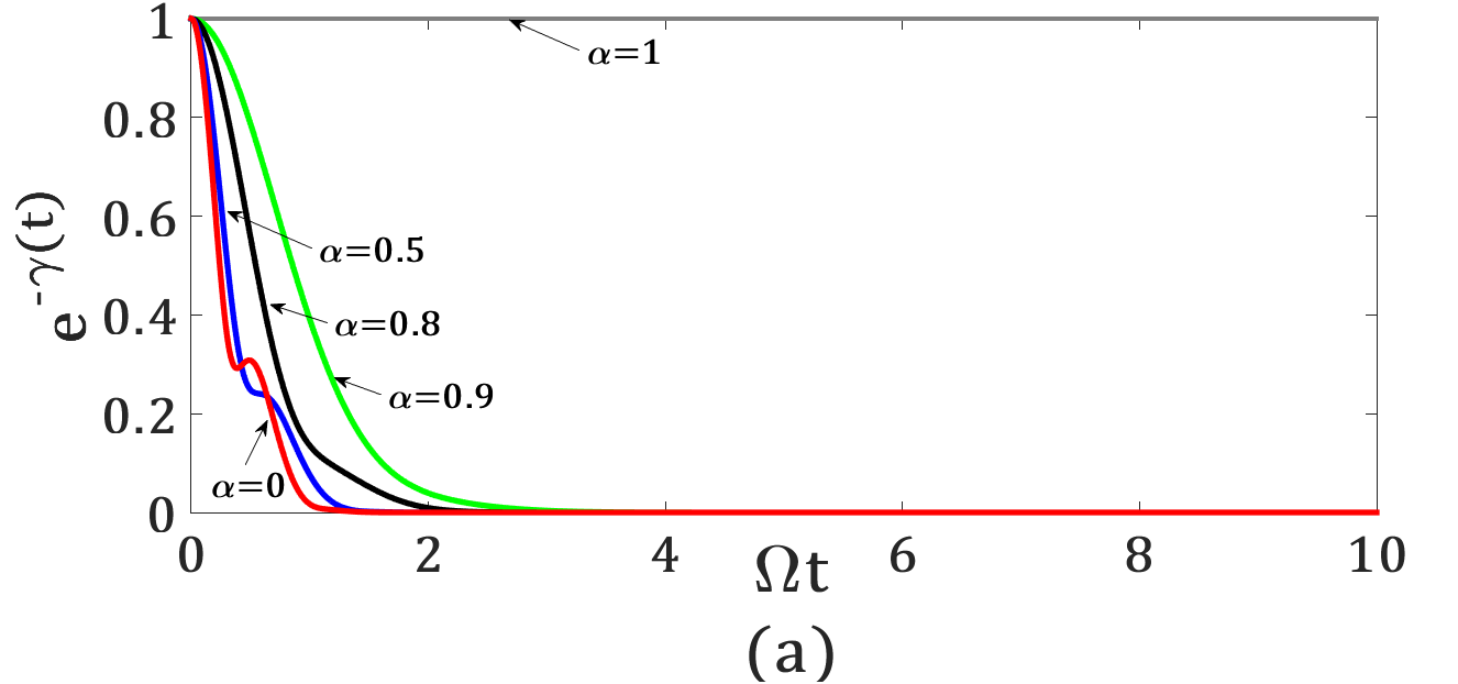
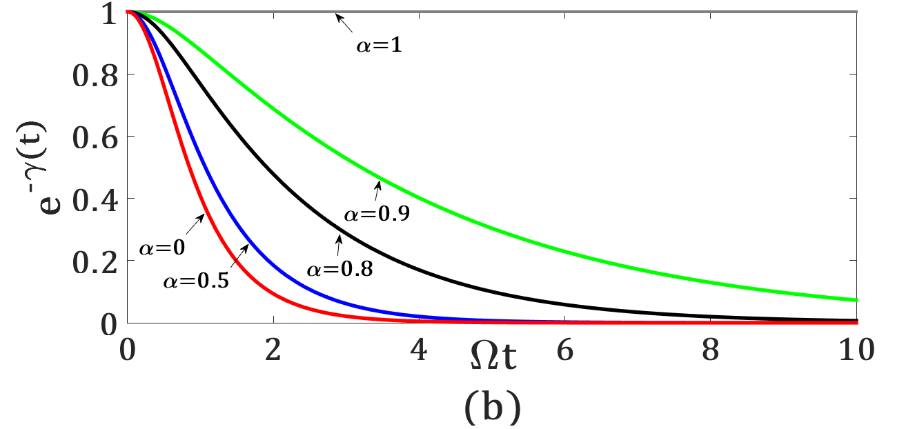
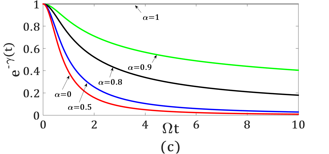
Figure 1: Time dependence of exponential of the total decoherence function $e^{-\gamma(t)}$ for initially correlated state for different values of $\alpha$ with $\beta\omega_{0}=1$ and the initial condition $\langle\sigma_{z}\rangle=0,\Omega\beta=1$ in all the (a) subohmic s=0.2 (b) ohmic s=1 and (c) superohmic s=2 cases.

Next, we assume the total system plus bath are in thermal equilibrium state at time $t<0$, and a measurement is made on such state at time $t=0$, such that we have at $t=0$ Nielsen ; muz ; mozorov

$$\rho(0)=\frac{1}{Z}\sum_{m}\Omega_{m}e^{-\beta H}\Omega_{m}^{\dagger}$$ (11)

where $\Omega_{m}$ are the projection operators on a desired state of system and/or bath. $Z$ is the normalization constant called as partition function. Now we make particular case of selective measurement, a projection by taking muz

$$\Omega_{m}=|\psi\rangle\langle\psi|\otimes I_{B}$$ (12)

where $I_{B}$ is the identity operation on the state of bath and $|\psi\rangle$ is a pure state of the qubit. Therefore we write

$$\rho(0)=|\psi\rangle\langle\psi|\otimes\rho_{B}(\psi)$$ (13)

where $\rho_{B}(\psi)=\frac{1}{Z}\langle\psi|e^{-\beta H}|\psi\rangle$ represents the density matrix of the bath and clearly depends on the state of the qubit $|\psi\rangle$.

$$\rho_{s}(t) = {\rm Tr}_{B}[U(t)\rho(0)U(t)^{\dagger}]$$ (14)

$$= {\rm Tr}_{B}[e^{\sigma^{z}\hat{\Lambda}(t)}|\psi\rangle\langle\psi|\otimes\rho_{B}(\psi)e^{-\sigma^{z}\hat{\Lambda}(t)}]$$ (15)

Now to evaulate the above expression, we take the general state of the qubit as $|\psi\rangle=a|0\rangle+b|1\rangle$, while we relegate the derivation to appendix A, we write

$$\rho_{s}(t)=\begin{pmatrix}|a|^{2}&ab^{*}F(t)\\ ba^{*}F^{*}(t)&|b|^{2}\end{pmatrix}$$ (16)

where

$$\!\!\!F(t) = [\frac{|a|^{2}e^{-\beta\omega_{0}/2}e^{i(1-\alpha^{2})\Phi(t)}+|b|^{2}e^{\beta\omega_{0}/2}e^{-i(1-\alpha^{2})\Phi(t)}}{|a|^{2}e^{-\beta\omega_{0}/2}+|b|^{2}e^{\beta\omega_{0}/2}}]e^{-\gamma_{1}(t)}$$

with $\Phi(t)=\sum\limits_{k}\frac{4|g_{k}|^{2}}{\omega_{k}^{2}}\sin\omega_{k}t$. Using the fact $|a|^{2}+|b|^{2}=1$ and $\langle\sigma_{z}\rangle=|a|^{2}-|b|^{2}$, we can write

$$\frac{|a|^{2}e^{-\beta\omega_{0}/2}e^{i(1-\alpha^{2})\Phi(t)}+|b|^{2}e^{\beta\omega_{0}/2}e^{-i(1-\alpha^{2})\Phi(t)}}{|a|^{2}e^{-\beta\omega_{0}/2}+|b|^{2}e^{\beta\omega_{0}/2}}=\cos(1-\alpha^{2})\Phi(t)-i\frac{\sinh\frac{\beta\omega_{0}}{2}-\langle\sigma_{z}\rangle\cosh\frac{\beta\omega_{0}}{2}}{\cosh\frac{\beta\omega_{0}}{2}-\langle\sigma_{z}\rangle\sinh\frac{\beta\omega_{0}}{2}}\sin(1-\alpha^{2})\Phi(t).$$ (18)

In order to get dephasing or time dependent frequency shift explicity we define

$$\tan[\chi(t)]=\frac{\sinh(\beta\omega_{0}/2)-\langle\sigma_{z}\rangle\cosh(\beta\omega_{0}/2)}{\cosh(\beta\omega_{0}/2)-\langle\sigma_{z}\rangle\sinh(\beta\omega_{0}/2)}\tan[(1-\alpha^{2})\Phi(t)]$$ (19)

so that $F(t)$ simplifies to $F(t)=e^{i\chi(t)}e^{-\gamma_{1}(t)-\gamma_{c}(t)}=e^{i\chi(t)-\gamma(t)}$ with $\gamma(t)=\gamma_{1}(t)+\gamma_{c}(t)$ and

$$\gamma_{c}(t)=-\frac{1}{2}\ln\Bigg{[}1-\frac{(1-\langle\sigma_{z}\rangle^{2})\sin^{2}[(1-\alpha^{2})\Phi(t)]}{\Big{(}\cosh(\beta\omega_{0}/2)-\langle\sigma_{z}\rangle\sinh(\beta\omega_{0}/2)\Big{)}^{2}}\Bigg{]}$$ (20)

The term $\gamma_{1}(t)$ represents the decoherence due to vaccum and thermal fluctuations of the bath while $\gamma_{c}(t)$ represents the decoherence due to initial correlations of the composite system. Thus we see that the decoherence function $\gamma_{1}(t)$ gets scaled by factor of $1-\alpha^{2}$ while as a different functional dependence on $\alpha$ is found for $\gamma_{c}(t)$.The reduced dynamics of $\mathcal{PT}$-symmetric qubit can be calculated as $T^{-1}\rho_{s}(t)T$.

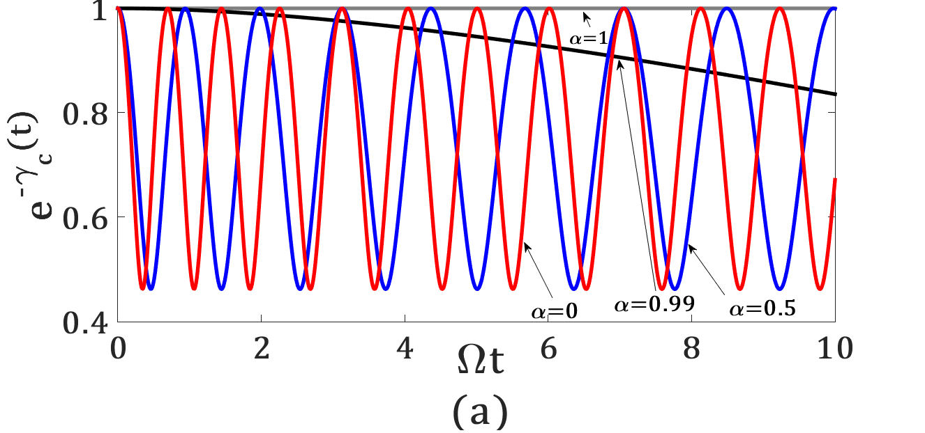
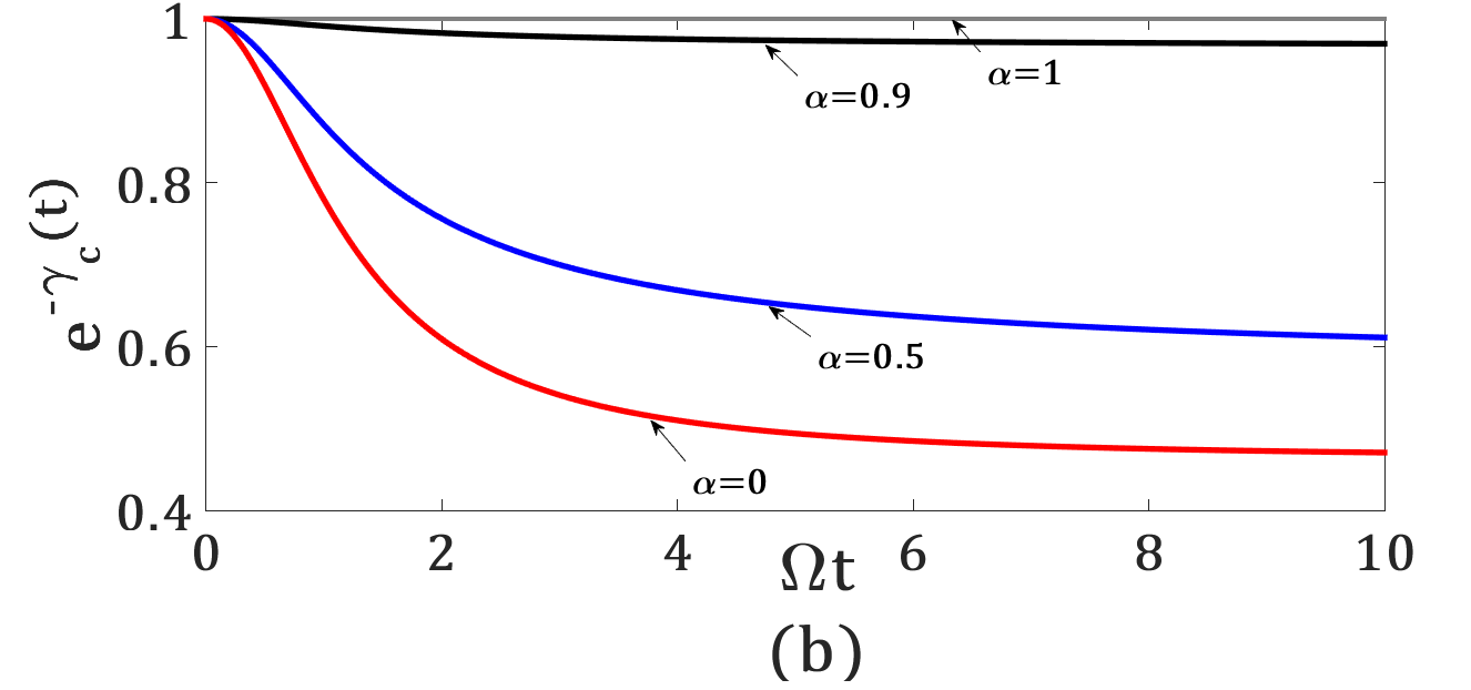
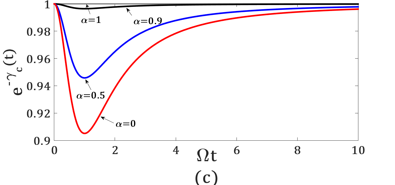
Figure 2: Time dependence of exponential of the decoherence due to initial correlations $e^{-\gamma_{c}(t)}$ for different values of $\alpha$ with $\beta\omega_{0}=1$ and the initial condition $\langle\sigma_{z}\rangle=0,\Omega\beta=1$ in all the (a) subohmic s=0.2 (b) ohmic s=1 and (c) superohmic s=2 cases.

Next, in order to understand the effect of parameter $\alpha$ on decoherence dynamics, we define bath spectral density function $J(\omega)=\sum_{k}4|g_{k}|^{2}\delta(\omega-\omega_{k})$. It is convienent to describe $J(\omega)$ phenomenologically by assuming the power law form with certian frequency cut-off. Therefore we write $J(\omega)=\lambda_{s}(\omega/\Omega)^{s}\Omega e^{-\omega/\Omega}$ where $\lambda_{s}$ is the dimensionless coupling constant and $\Omega$ is the cutt-off frequency. The values $s$ determine the nature of the bath, if $s=1$, we call it as ohmic bath while $s<1$ and $s>1$ are called as sub-ohmic and super-ohmic baths respectively.

Figure 1 shows the variation of total decoherence $e^{-\gamma(t)}$ with respect to $\Omega t$ for different values of $\alpha$ in the subohmic $s<1$ , ohmic $s=1$ and superohmic $s=2$ regimes, where $\gamma(t)=\gamma_{1}(t)+\gamma_{c}(t)$. We see from figure 1(a), that for $\alpha=0$ we observe strong oscillations of $e^{-\gamma(t)}$. However as $\alpha$ increases from 0 to 1 , the oscillations freeze out. The oscillations observed in $e^{-\gamma(t)}$ are due the initial correlations in the subohmic regime as can be seen from figure 2(a). The period of oscillations increases from finite to infinite value, thus freeze out at the value of $\alpha=1$. These features are due to the fact that it takes a longer time for the system to complete one Hilbert space oscillation resulting in extremely slow dynamics near the boundary $\alpha=1$ on which the dynamics completely freezes.

Next, we turn to the ohmic case $s=1$. In this case, using the explicit form of $J(\omega)$, we can write the explicit form of decoherence functions in closed form as mozorov

$$\gamma_{1}(t) = (1-\alpha^{2})\left[\frac{\lambda_{1}}{2}\ln(1+\Omega^{2}t^{2})\right.$$

$$\left.\!\!\!\!+2\lambda_{1}[\ln\Gamma(1+1/\Omega\beta)-\frac{1}{2}\ln|\Gamma(1+1/\Omega\beta+it/\beta)|^{2}\right]$$

$$\Phi(t) = \lambda_{1}\tan^{-1}(\Omega t)$$ (21)

Figures 1(b) and 2(b) show the variation of $e^{-\gamma(t)}$ and $e^{-\gamma_{c}(t)}$ with respect to $\Omega t$ for different values of $\alpha$. It can be seen from the plot as the hermiticity parameter increases from 0 to 1, the slowing down of decoherence is observed. It is noted the sudden transition at $\alpha=1$ with no decoherence at all. This feature can be attributed to the frozen dynamics of the system Hamiltonian at $\alpha=1$.

For superohmic case, no oscillatory behaviour is found unlike sub ohmic case see figures 1(c) and 2(c). This is in complete contrast with the sub ohmic case where the oscillation time period becomes infinite. Although, in both super-ohmic and sub-ohmic cases as dynamics kicks off at $t=0$ the bath has a rapid correlation dependent effect on the qubit explaining the initial minima in the graphs, but in long time limit the qubit settles in a steady state, completely independent of the initial dynamics for superohmic case, while as no such steady state is formed for sub-ohmic case. Nevertheless, both the dynamics have the same physical consequences that intial correlations disappear. In other words it would not matter whether initially the system was prepared independently or a projective measurement was made on the thermalized system and bath, both will result in approximately same dynamics near the boundary of separation of physical and unphysical hamiltonians.

IV Conclusions

In conclusion, we studied a $\mathcal{PT}$-symmetric qubit coupled to a bosonic bath. Using a cannonical transformation, we mapped the $\mathcal{PT}$-symmetric model to well known spin-boson model which is a purely dephasing model. Using projective measurement on system only in a thermalized state of system plus bath, we arrive at correlated initial state with bath state depending on the degrees of freedom of the system. We show that the decoherence due to these initial correlations are strongly modified in the sub-ohmic regime. Moreover, it is shown that total decoherence is slowed down with the increase in the hermiticity parameter $\alpha$. At the transition point that seperates the hermitian and non-hermitian regimes, the dynamics of the qubit freezes out making the qubit more robust against external perturbations. A similiar dynamics is also observed in Kibble-Zurek mechanism applied to one dimensional Ising model Ising . We see that the decoherence due to initial correlations in all the subohmic, ohmics and super-ohmic cases is suppressed in the physically relevant regime for $\alpha$ near to 1. This results in approximately the same dynamics of an initially correlated and an uncorrelated state.

Appendix A

In this appendix, we derive the time evolution of the reduced density matrix $\rho_{s}(t)$ given in the equation 16. Since the Hamiltonian $\tilde{H}$ given in equation 4 is a purely dephasing model, which results in no dynamics of the diagonal terms of the density matrix $\rho_{s}(t)$. Observing that

$$e^{-\beta\tilde{H}}\mid 1\rangle =e^{-\beta\mu}e^{-\beta H^{+}}\mid 1\rangle$$

$$e^{-\beta\tilde{H}}\mid 0\rangle =e^{\beta\mu}e^{-\beta H^{-}}\mid 0\rangle$$

with $H^{\pm}=\sum\limits_{k}\omega_{k}b_{k}^{\dagger}b_{k}\pm\sum\limits_{k}E(g_{k}b_{k}+g_{k}^{*}b_{k}^{\dagger})$ and $\mu=\frac{\omega_{o}}{2}$, we can write the $\langle 1|\rho_{s}(t)|0\rangle=\rho_{s}^{10}(t)$ as

$$\rho_{s}^{10}(t) = \frac{ab^{*}}{Z}(|a|^{2}e^{-\beta\mu}{\rm Tr}_{B}[e^{2\hat{\Lambda}(t)}e^{-\beta H^{+}}]$$ (22)

$$~{}~{}~{}~{}+|b|^{2}e^{\beta\mu}{\rm Tr}_{B}[e^{2\hat{\Lambda}(t)}e^{-\beta H^{-}}])$$

where the partition function $Z$ is given by

$$Z=|a|^{2}e^{-\beta\mu}{\rm Tr}_{B}[e^{-\beta H^{+}}]+|b|^{2}e^{\beta\mu}{\rm Tr}_{B}[e^{-\beta H^{-}}]$$

Next we define a unitary transformation $O_{\pm}=\exp[\pm\sum_{k}\frac{E}{\omega_{k}}(g_{k}b_{k}-g_{k}^{*}b_{k}^{\dagger})]$ such that $H^{\pm}=O_{\pm}^{-1}(H_{B}-\xi)O_{\pm}$ with $\xi=\sum\limits_{k}E^{2}\frac{|g_{k}^{2}|}{\omega_{k}}$ and $2\hat{\Lambda}(t)=O_{\pm}^{-1}[2\hat{\Lambda}(t)\pm iE^{2}\Phi(t)]O_{\pm}$. Therefore, we write

$$\!\!\!\!{\rm Tr}_{B}[e^{2\hat{\Lambda}(t)}e^{-\beta H^{\pm}}]$$

$$={\rm Tr}_{B}[O_{\pm}^{-1}e^{2\hat{\Lambda}(t)\pm iE^{2}\Phi(t)}O_{\pm}O_{\pm}^{-1}e^{-\beta H_{B}+\beta\xi}O_{\pm}]$$

$$={\rm Tr}_{B}[O_{\pm}^{-1}e^{2\hat{\Lambda}(t)\pm iE^{2}\Phi(t)}e^{-\beta H_{B}+\beta\xi}O_{\pm}]$$

$$=e^{\pm i(1-\alpha^{2})\Phi(t)}Z_{B}e^{-\gamma_{1}(t)}e^{\beta\xi}$$

where $Z_{B}={\rm Tr}_{B}[e^{-\beta H_{B}}]$. This makes partition function $Z$ to be

$$Z=Z_{B}e^{\beta\xi}(|a|^{2}e^{-\beta\mu}+|b|^{2}e^{\beta\mu})$$

Substituting all the above results in the expression for the off diagonal element $\rho_{s}^{10}(t)$ we have

$$\rho_{s}^{10}(t) =ab^{*}\frac{|a|^{2}e^{-\beta\frac{\omega_{0}}{2}}e^{i(1-\alpha^{2})\Phi(t)}+|b|^{2}e^{\beta\frac{\omega_{0}}{2}}e^{-i(1-\alpha^{2})\Phi(t)}}{|a|^{2}e^{-\beta\frac{\omega_{0}}{2}}+|b|^{2}e^{\beta\frac{\omega_{0}}{2}}}e^{-\gamma_{1}(t)}$$

References

• (1) C. M. Bender, Rep. Prog. Phys. 70, 947 (2007).
• (2) L. Feng, et. al. Nature Materials 12, 108–113 (2013)
• (3) S. Longhi, Phys.Rev. Lett. 105, 013903 (2010); S, Longhi and G. Della Valle, Phys. Rev. A 85, 012112 (2012).
• (4) P. A. M. Dirac, Math. Proc. Cambridge Philos. Soc. 35, 416 (1939).
• (5) J. von Neumann, Mathematical Foundations of Quantum Mechanics (Princeton University Press, 1955).
• (6) C. E. R$\ddot{u}$ter, K. G. Makris, R. El-Ganainy, D. N. Christodoulides, M. Segev, and D. Kip, Nat. Phys. 6, 192 (2010).
• (7) A. Guo, G. J. Salamo, D. Duchesne, R. Morandotti, M. Volatier- Ravat, V. Aimez, G. A. Siviloglou, and D. N. Christodoulides, Phys. Rev. Lett. 103, 093902 (2009).
• (8) X.-Y. LΓΌ, H. Jing, J.-Y. Ma, and Y. Wu, Phys. Rev. Lett. 114, 253601 (2015).
• (9) B. Peng et al., Nat. Phys. 10, 394 (2014).
• (10) B. Gardas, S. Deffner, and A. Saxena , Phys. Rev. A 94, 040101(R) (2016).
• (11) H.P. Beuer and F. Petruccione, The Theory of Open Quantum systems (Oxford, New York: Oxford University Press) 2000.
• (12) M. Schlosshauer, Rev. Mod. Phys. 76, 1267 (2005).
• (13) W. H. Zurek Rev. Mod. Phys. 75, 715 (2003) .
• (14) J. T. Barreiro , P. Schindler ,O. GΓΌhne ,T. Monz ,M. Chwalla, C. F. Roos , M. Hennrich and R. Blatt, Nature Phys. 6, 943 (2010).
• (15) S. Schneider and G. J. Milburn Phys. Rev. A 57, 3748 (1998).
• (16) Q. A. Turchette , C. J.Myatt, B. E. King , C. A. Sackett , D. Kielpinski, W. M. Itano , C. Monroe and D. J. Wineland, Phys. Rev. A, 62, 053807 (2000).
• (17) S. Diehl, A. Micheli, A. Kantian, B. Kraus, H. Buechler and P. Zoller, Nature Phys. 4, 878 (2008).
• (18) F. Verstraete, M. M. Wolf and J. I. Cirac, Nat. Phys. 5, 633 (2009) .
• (19) H. Weimer, M. MΓΌller, I. Lesanovsky, P. Zoller and H. P. BΓΌchler, Nature Phys. 6, 382 (2010).
• (20) B. Bellomo, R. Lo Franco, and G. Compagno Phys. Rev. Lett. 99, 160502 (2007).
• (21) R. Lo Franco, New J. Phys. 17, 081004 (2015).
• (22) F. Brito and T. Werlang, New J. Phys. 17, 072001 (2015)
• (23) Z.-X. Man, Y.-J. Xia, and R. Lo Franco, Phys. Rev. A 92, 012315 (2015).
• (24) E. M. Laine, H. P. Breuer, J. Piilo, C.-F. Li and G.-C. Guo, Phys. Rev. Lett. 108, 210402 (2012).
• (25) B. Peng, et. al. Nat. Phys. 10, 394–398 (2014).
• (26) A. K. Pati, Pramana 73, 3 (2009).
• (27) K. Kraus, States, Effects, and Operations, (Springer-Verlag ) 1983.
• (28) M. Q. Lone, C. Nagele, B. Weslake, T. Byrnes, arXiv:1711.10257
• (29) V. G. Morozov, S. Mathey, and G. R$\ddot{o}$pke, Phys. Rev. A 85, 022101 (2012).
• (30) T. W. B. Kibble, J. Phys. A: Math. Gen. 9, 1387 (1976); W. H. Zurek, Nature (London) 317, 505 (1985).