A distributed Lagrange formulation of the Finite Element Immersed Boundary Method for fluids interacting with compressible solids.

Abstract

We present a distributed Lagrange multiplier formulation of the Finite Element Immersed Boundary Method to couple incompressible fluids with compressible solids. This is a generalization of the formulation presented in Heltai and Costanzo (2012), that offers a cleaner variational formulation, thanks to the introduction of distributed Lagrange multipliers, that acts as intermediary between the fluid and solid equations, keeping the two formulation mostly separated. Stability estimates and a brief numerical validation are presented.

1 Introduction

Fluid-structure interaction (FSI) problems are everywhere in engineering and biological applications, and are often too complex to solve analytically.

Well established techniques, like the Arbitrary Lagrangian Eulerian (ALE) framework HughesLiuK.-1981-a , enable the numerical simulation of FSI problems by coupling computational fluid dynamics (CFD) and computational structural dynamics (CSD), through the introduction of a deformable fluid grid, whose movement at the interface is driven by the coupling with the CSD simulation, while the interior is deformed arbitrarily, according to some smooth deformation operator.

Although this technique has reached a great level of robustness, whenever changes of topologies are present in the physics of the problem, or when freely floating objects (possibly rotating) are considered, a deforming fluid grid that follows the solid may no longer be a feasible solution strategy.

The Immersed Boundary Method (IBM), introduced by Peskin in the seventies Peskin-1977-a to simulate the interaction of blood flow with heart valves, addressed this issue by reformulating the coupled FSI problem as a “reinforced fluid” problem, where the CFD system is solved everywhere (including in the regions occupied by the solid), and the presence of the solid is taken into account in the fluid as a (singular) source term (see Peskin-2002-a for a review).

In the original IBM, the body forces expressing the FSI are determined by modeling the solid body as a network of elastic fibers with a contractile element, where each point of the fiber acts as a singular force field (a Dirac delta distribution) on the fluid.

Finite element variants of the IBM were first proposed, almost simultaneously, by BoffiGastaldi-2003-a , WangLiu-2004-a , and ZhangGerstenbergerWang-2004-a . However, only BoffiGastaldi-2003-a exploited the variational definition of the Dirac delta distribution directly in the finite element (FE) approximations.

Such approximation was later generalized to thick hyper-elastic bodies (as opposed to fibers) BoffiGastaldiHeltaiPeskin-2008-a , where the constitutive behavior of the immersed solid is assumed to be incompressible and visco-elastic with the viscous component of the solid stress response being identical to that of the fluid.

In HeltaiCostanzo-2012-a , the authors present a formulation that is applicable to problems with immersed bodies of general topological and constitutive characteristics, without the use of Dirac delta distributions, and with interpolation operators between the fluid and the solid discrete spaces that guarantee semi-discrete stability estimates and strong consistency. Such formulation has been successfully used RoyHeltaiCostanzo-2015-a to match standard benchmark tests TurekHron-2006-a .

In this work we show how the incompressible version of the FSI model presented in HeltaiCostanzo-2012-a can be seen as a special case of the Distributed Lagrange Multiplier method, introduced in BoffiCavalliniGastaldi-2015-a , and we present a novel distributed Lagrange multiplier method that generalizes the compressible model introduced in HeltaiCostanzo-2012-a .

We provide a general variational framework for Immersed Finite Element Methods (IFEM) based on the distributed Lagrange multiplier formulation that is suitable for general fluid structure interaction problems.

2 Setting of the problem

Let $\Omega\subset\mathbb{R}^{d}$, with $d=2,3$, be a fixed open bounded polyhedral domain with Lipschitz boundary which is split into two time dependent subdomains $\Omega^{f}_{t}$ and $\Omega^{s}_{t}$, representing the fluid and the solid regions, respectively. Hence $\Omega$ is the interior of $\overline{\Omega}^{f}_{t}\cup\overline{\Omega}^{s}_{t}$ and we denote by $\Gamma_{t}=\overline{\Omega}^{f}_{t}\cap\overline{\Omega}^{s}_{t}$ the moving interface between the fluid and the solid regions. For simplicity, we assume that $\Gamma_{t}\cap\partial\Omega=\emptyset$.

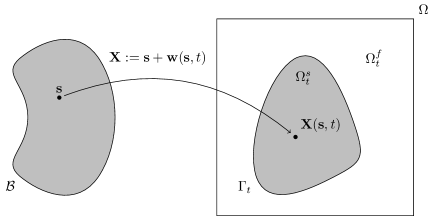
Figure 1: Geometrical configuration of the FSI problem

The current position of the solid $\Omega^{s}_{t}$ is the image of a reference domain $\mathcal{B}$ through a mapping $\mathbf{X}:\mathcal{B}\to\Omega^{s}_{t}$. The displacement of the solid is indicated by $\mathbf{w}$ and for any point $\mathbf{x}\in\Omega^{s}_{t}$ we have $\mathbf{x}=\mathbf{X}(\mathbf{s},t)=\mathbf{X}_{0}(\mathbf{s})+\mathbf{w}(\mathbf{s},t)$ for some $\mathbf{s}\in\mathcal{B}$, where $\mathbf{X}_{0}:\mathcal{B}\to\Omega_{0}^{s}$ denotes the mapping providing the initial configuration of $\Omega^{s}_{t}$. For convenience, we assume that the reference domain $\mathcal{B}$ coincides with $\Omega_{0}^{s}$ so that $\mathbf{X}(s,t)=\mathbf{s}+\mathbf{w}(\mathbf{s},t)$ and $\mathcal{B}\subset\Omega$. From the above definitions, $\mathbb{F}=\mathop{\nabla_{s}}\nolimits\mathbf{X}=\mathbb{I}+\mathop{\nabla_{s}}\nolimits\mathbf{w}$ stands for the deformation gradient and $J=\mathop{\rm{det}}\nolimits(\mathbb{F})$ for its Jacobian.

We denote by $\mathbf{u}_{f}:\Omega\to\mathbb{R}^{d}$ and $p_{f}:\Omega\to\mathbb{R}$ the fluid velocity and pressure and assume that the solid velocity $\mathbf{u}_{s}$ is equal to the material velocity of the solid, that is

$$\mathbf{u}_{s}(\mathbf{x},t)=\frac{\partial\mathbf{X}(\mathbf{s},t)}{\partial t}\Big{|}_{\mathbf{x}=\mathbf{X}(\mathbf{s},t)}=\frac{\partial\mathbf{w}(\mathbf{s},t)}{\partial t}\Big{|}_{\mathbf{x}=\mathbf{X}(\mathbf{s},t)}.$$ (1)

We indicate with generic symbols $\mathbf{u},p,\rho$ the Eulerian fields, depending on $\mathbf{x}$ and $t$, which describe the velocity, pressure, and density, respectively, of a material particle (be it solid or fluid). By $\dot{\mathbf{u}}$ we denote the material derivative of $\mathbf{u}$, which in Eulerian coordinates is expressed by

$$\dot{\mathbf{u}}(\mathbf{x},t)=\frac{\partial\mathbf{u}}{\partial t}(\mathbf{x},t)+\mathbf{u}(\mathbf{x},t)\cdot\mathop{\boldsymbol{\nabla}}\nolimits\mathbf{u}(\mathbf{x},t).$$ (2)

In the Lagrangian framework, the material derivative coincides with the partial derivative with respect to time, so that

$$\dot{\mathbf{w}}(\mathbf{s},t)=\partial\mathbf{w}(\mathbf{s},t)/\partial t.$$

Continuum mechanics models are based on the conservation of three main properties: linear momentum, angular momentum, and mass.

When expressed in Lagrangian coordinates, mass conservation is guaranteed if the reference mass density $\rho_{0}$ is time independent. If expressed in Eulerian coordinates, however, mass conservation takes the form

$$\dot{\rho}+\rho\mathop{\rm{div}}\nolimits\mathbf{u}=0\quad\text{in }\Omega,$$ (3)

and should be included in the system’s equations.

Conservation of both momenta can be expressed, in Eulerian coordinates, as:

$$\rho\dot{\mathbf{u}}=\mathop{\rm{div}}\nolimits\boldsymbol{\sigma}+\rho\mathbf{b}\quad\text{in }\Omega,$$ (4)

where $\rho$ is the mass density distribution, $\mathbf{u}$ the velocity, $\boldsymbol{\sigma}$ is the Cauchy stress tensor (its symmetry implies that conservation of angular momenta is guaranteed by equation (4)), and $\mathbf{b}$ describes the external force density per unit mass acting on the system. Such a description is common to all continuum mechanics models (see, for example, Gurtin-1982-a ). The equations for fluids and solids are different according to their constitutive behavior, i.e., according to how $\boldsymbol{\sigma}$ relates to $\mathbf{u},\mathbf{w}$, or $p$.

If the material is incompressible, it can be shown that $\mathop{\rm{div}}\nolimits\mathbf{u}=0$ everywhere, and the material derivative of the density is constantly equal to zero (from equation (3)). Notice that this does not imply that $\rho$ is constant (neither in time nor in space), and it is still in general necessary to include equation (3) in the system.

For incompressible materials, however, the volumetric part of the stress tensor can be interpreted as a Lagrange multiplier associated with the incompressibility constraints. For incompressible fluids, the stress is decomposed into $\boldsymbol{\sigma}_{f}=-p_{f}\mathbb{I}+\nu_{f}\mathbf{D}\mathbf{u}_{f}$ where $\mathbf{u}_{f}$ is the fluid velocity, $p_{f}$ the pressure, $\nu_{f}>0$ is the viscosity coefficient and $\mathbf{D}\mathbf{u}_{f}=(1/2)\left(\mathop{\boldsymbol{\nabla}}\nolimits\mathbf{u}_{f}+(\mathop{\boldsymbol{\nabla}}\nolimits\mathbf{u}_{f})^{\top}\right)$.

Hence the equations describing the fluid motion are the well-known Navier–Stokes equations, that is:

$$\rho_{f}\dot{\mathbf{u}}_{f}-\mathop{\rm{div}}\nolimits(\nu_{f}\mathbf{D}\mathbf{u}_{f})+\mathop{\nabla}\nolimits p_{f}=\rho_{f}\mathbf{b} \text{in }\Omega^{f}_{t}$$ (5)

$$\mathop{\rm{div}}\nolimits\mathbf{u}_{f}=0 \text{in }\Omega^{f}_{t},$$

where we assumed that $\rho_{f}$ is constant throughout $\Omega^{f}_{t}$.

As far as the solid is concerned, we assume that it is composed by a viscous elastic material so that the Cauchy stress tensor can be decomposed into the sum of two contributions: a viscous part and a pure elastic part, as follows

$$\boldsymbol{\sigma}_{s}=\boldsymbol{\sigma}_{s}^{v}+\boldsymbol{\sigma}_{s}^{e}=\nu_{s}\mathbf{D}\mathbf{u}_{s}+\boldsymbol{\sigma}_{s}^{e}.$$ (6)

Here $\mathbf{u}_{s}$ is the solid velocity, $\nu_{s}\geq 0$ is the solid viscosity coefficient and $\boldsymbol{\sigma}_{s}^{e}$ denotes the elastic part of the solid Cauchy stress tensor. We assume this elastic part to behave hyper-elastically, i.e., we assume that there exists an elastic potential energy density $W(\mathbb{F})$ such that $W(\mathbf{R}\mathbb{F})=W(\mathbb{F})$ for any rotation $\mathbf{R}$, that represents the amount of elastic energy stored in the current solid configuration, and that depends only on its deformation gradient $\mathbb{F}=\mathop{\nabla_{s}}\nolimits\mathbf{X}$.

When expressed in Lagrangian coordinates, a possible measure for the elastic part of the stress is the so called first Piola–Kirchhoff stress tensor, defined as the Fréchet derivative of $W$ w.r.t. to $\mathbb{F}$, i.e.:

$$\mathbb{P}_{s}^{e}:=\frac{\partial W}{\partial\mathbb{F}}.$$ (7)

The first Piola–Kirchhoff stress tensor allows one to express the conservation of linear momentum in Lagrangian coordinates as

$$\rho_{s_{0}}\ddot{\mathbf{w}}=\mathop{\mathbf{Div}}\nolimits(\mathbb{P})+\rho_{s_{0}}\mathbf{B}\quad\text{ in }\mathcal{B},$$ (8)

where, similarly to its Eulerian counterpart, we assume that $\mathbb{P}$ is decomposed in an additive way into its viscous part $\mathbb{P}_{s}^{v}$ and into its elastic part $\mathbb{P}_{s}^{e}$, defined in equation (7).

For any portion $\mathcal{P}\subset\mathcal{B}$ of the solid (with outer normal $\mathbf{N}$) deformed to $\mathcal{P}_{t}$ (with outer normal $\mathbf{n}$), the following relation between $\mathbb{P}$ and $\boldsymbol{\sigma}$ holds:

$$\int_{\mathcal{P}}\mathbb{P}\mathbf{N}\,\mathbf{d}\Gamma_{s}=\int_{\mathcal{P}_{t}}\boldsymbol{\sigma}\mathbf{n}\,\mathbf{d}\Gamma_{x},\qquad\forall\mathcal{P}\subset\mathcal{B},\qquad\mathcal{P}_{t}:=\mathbf{X}(\mathcal{P},t),$$ (9)

that is, we can express pointwise the viscous part of the solid stress in Lagrangian coordinates by rewriting the first Piola–Kirchhoff stress $\mathbb{P}^{v}_{s}$ in terms of $\boldsymbol{\sigma}_{s}^{v}:=\nu_{s}\mathbf{D}\mathbf{u}_{s}$, and the hyper-elastic part of the solid stress in Eulerian coordinates by expressing the Cauchy stress $\boldsymbol{\sigma}_{s}^{e}$ in terms of $\mathbb{P}_{s}^{e}:=\partial W/\partial\mathbb{F}$:

$$\mathbb{P}^{v}_{s}(\mathbf{s},t) :=J^{\phantom{-1}}\boldsymbol{\sigma}_{s}^{v}(\mathbf{x},t)\mathbb{F}^{-\top}(\mathbf{s},t) \quad\text{for }\mathbf{x}=\mathbf{X}(\mathbf{s},t)$$ (10)

$$\boldsymbol{\sigma}^{e}_{s}(\mathbf{x},t) :=J^{-1}\mathbb{P}_{s}^{e}(\mathbf{s},t)\ \mathbb{F}^{\top}(\mathbf{s},t)\phantom{-} \quad\text{for }\mathbf{x}=\mathbf{X}(\mathbf{s},t).$$

With these definitions, the conservation of linear momentum for the solid equation can be expressed either in Lagrangian coordinates as

$$\rho_{s_{0}}\ddot{\mathbf{w}}=\mathop{\mathbf{Div}}\nolimits\mathbb{P}^{v}_{s}+\mathop{\mathbf{Div}}\nolimits\frac{\partial W}{\partial\mathbb{F}}+\rho_{s_{0}}\mathbf{B}\quad\text{ in }\mathcal{B}$$ (11)

or in Eulerian coordinates as

$$\rho_{s}\dot{\mathbf{u}}_{s}-\mathop{\rm{div}}\nolimits(\nu_{s}\mathbf{D}\mathbf{u}_{s})-\mathop{\rm{div}}\nolimits\boldsymbol{\sigma}_{s}^{e}=\rho_{s}\mathbf{b}\quad\text{in }\Omega^{s}_{t}.$$ (12)

Notice that the conservation of mass for the solid equation is a simple kinematic identity that derives from the fact that $\rho_{s_{0}}$ does not depend on time, i.e., we have

$$\frac{\dot{\rho}_{s}}{\rho_{s}}+\mathop{\rm{div}}\nolimits\mathbf{u}_{s}=0\qquad\text{in }\Omega^{s}_{t},$$ (13)

or, equivalently,

$$\rho_{s}(\mathbf{x},t)=\rho_{s_{0}}(\mathbf{s})/J(\mathbf{s},t)\quad\text{for }\mathbf{x}=\mathbf{X}(\mathbf{s},t),$$ (14)

that is:

$$\mathop{\rm{div}}\nolimits\mathbf{u}_{s}(\mathbf{x},t)=\frac{\dot{J}}{J}(\mathbf{s},t)\quad\quad\text{for }\mathbf{x}=\mathbf{X}(\mathbf{s},t).$$ (15)

The equations in the solid and in the fluid are coupled through interface conditions along $\Gamma_{t}$, which enforce the continuity of the velocity, corresponding to the no-slip condition between solid and fluid, and the balance of the normal stress:

$$\mathbf{u}_{f}=\mathbf{u}_{s} \text{on }\Gamma_{t}$$ (16)

$$\boldsymbol{\sigma}_{f}\mathbf{n}_{f}+\boldsymbol{\sigma}_{s}\mathbf{n}_{s}=0 \text{on }\Gamma_{t},$$

where $\mathbf{n}_{f}$ and $\mathbf{n}_{s}$ denote the outward unit normal vector to $\Omega^{f}_{t}$ and $\Omega^{s}_{t}$, respectively.

The system is complemented with initial and boundary conditions. The boundary $\partial\Omega$ is split into two parts $\partial\Omega_{D}$ and $\partial\Omega_{N}$, where Dirichlet and Neumann conditions are imposed, respectively, with $\partial\Omega_{D}\cap\partial\Omega_{N}=\emptyset$. Since we assumed that $\partial\Omega\cap\Gamma_{t}=\emptyset$, the initial and boundary conditions are given by:

$$\mathbf{u}_{f}(0)=\mathbf{u}_{f0} \text{in }\Omega_{0}^{f}$$ (17)

$$\mathbf{u}_{s}(0)=\mathbf{u}_{s0} \text{in }\Omega_{0}^{s}$$

$$\mathbf{X}(0)=\mathbf{X}_{0} \text{in }\mathcal{B}$$

$$\mathbf{u}_{f}=\mathbf{u}_{g} \text{on }\partial\Omega_{D}$$

$$(\nu_{f}\mathbf{D}\mathbf{u}_{f}-p_{f}\mathbb{I})\mathbf{n}_{f}=\boldsymbol{\tau}_{g} \text{on }\partial\Omega_{N}.$$

In the following, we shall consider $\mathbf{u}_{g}=0$ on $\partial\Omega_{D}$, for simplicity, and we define the space $H^{1}_{0,D}(\Omega)^{d}$ as the space of functions in $H^{1}(\Omega)^{d}$ such that their trace on $\partial\Omega_{D}$ is zero.

By multiplying by $\mathbf{v}\in H^{1}_{0,D}(\Omega)^{d}$ the first equation in (5) and (12), integrating by part and using the second interface condition in (16), we arrive at the following weak form of the fluid-structure interaction problem: find $\mathbf{u}_{f}$, $p_{f}$, $\mathbf{u}_{s}$, and $\mathbf{w}$ such that (1), (16)₁ and (17) are satisfied and it holds:

$$\int_{\Omega^{f}_{t}} \rho_{f}(\dot{\mathbf{u}}_{f}-\mathbf{b})\mathbf{v}\,\mathrm{d}\mathbf{x}+\int_{\Omega^{f}_{t}}\nu_{f}\mathbf{D}\mathbf{u}_{f}:\mathbf{D}\mathbf{v}\,\mathrm{d}\mathbf{x}-\int_{\Omega^{f}_{t}}p_{f}\mathop{\rm{div}}\nolimits\mathbf{v}\,\mathrm{d}\mathbf{x}$$ (18)

$$+\int_{\Omega^{s}_{t}}\rho_{s}(\dot{\mathbf{u}}_{s}-\mathbf{b})\mathbf{v}\,\mathrm{d}\mathbf{x}+\int_{\Omega^{s}_{t}}\nu_{s}\mathbf{D}\mathbf{u}_{s}:\mathbf{D}\mathbf{v}\,\mathrm{d}\mathbf{x}+\int_{\Omega^{s}_{t}}\boldsymbol{\sigma}_{s}^{e}:\mathbf{D}\mathbf{v}\,\mathrm{d}\mathbf{x}$$

$$\qquad\qquad=\int_{\partial\Omega_{N}}\boldsymbol{\tau}_{g}\cdot\mathbf{v}\,\mathrm{da}\qquad\forall\mathbf{v}\in H^{1}_{0,D}(\Omega)^{d}$$

$$\int_{\Omega^{f}_{t}} \mathop{\rm{div}}\nolimits\mathbf{u}_{f}q_{f}\,\mathrm{d}\mathbf{x}=0\qquad\qquad\qquad\forall q_{f}\in L^{2}(\Omega^{f}_{t})$$

where the notation $\dot{\mathbf{u}}$ indicates the material derivative with respect to time. Using a fictitious domain approach, we transform problem (18) by introducing the following new unknowns. Thanks to the continuity condition for fluid and solid velocity, we define $\mathbf{u}\in H^{1}_{0,D}(\Omega)^{d}$ and $p\in L^{2}(\Omega)$ as

$$\mathbf{u}=\left\{\begin{array}[]{ll}\mathbf{u}_{f}&\text{in }\Omega^{f}_{t}\\ \mathbf{u}_{s}&\text{in }\Omega^{s}_{t}.\end{array}\right.,\qquad p=\left\{\begin{array}[]{ll}p_{f}&\text{in }\Omega^{f}_{t}\\ p_{s}=0&\text{in }\Omega^{s}_{t}.\end{array}\right..$$ (19)

Notice that the pressure field does not have any physical meaning in the solid, and it is (weakly) imposed to be zero.

Then we can write:

$$\int_{\Omega} \rho_{f}\dot{\mathbf{u}}\mathbf{v}\,\mathrm{d}\mathbf{x}+\int_{\Omega}\nu_{f}\mathbf{D}(\mathbf{u}):\mathbf{D}(\mathbf{v})\,\mathrm{d}\mathbf{x}-\int_{\Omega}p\mathop{\rm{div}}\nolimits\mathbf{v}\,\mathrm{d}\mathbf{x}+\int_{\Omega^{s}_{t}}(\rho_{s}-\rho_{f})\dot{\mathbf{u}}\mathbf{v}\,\mathrm{d}\mathbf{x}$$ (20)

$$+\int_{\Omega^{s}_{t}}(\nu_{s}-\nu_{f})\mathbf{D}\mathbf{u}:\mathbf{D}\mathbf{v}\,\mathrm{d}\mathbf{x}+\int_{\Omega^{s}_{t}}\boldsymbol{\sigma}_{s}^{e}:\mathbf{D}\mathbf{v}\,\mathrm{d}\mathbf{x}+\int_{\Omega^{s}_{t}}p\mathop{\rm{div}}\nolimits\mathbf{v}\,\mathrm{d}\mathbf{x}$$

$$\qquad\qquad=\int_{\Omega}\mathbf{f}\mathbf{v}\,\mathrm{d}\mathbf{x}+\int_{\partial\Omega_{N}}\boldsymbol{\tau}_{g}\cdot\mathbf{v}\,\mathrm{da} \forall\mathbf{v}\in H^{1}_{0,D}(\Omega)^{d}$$

$$\int_{\Omega} \mathop{\rm{div}}\nolimits\mathbf{u}\,q\,\mathrm{d}\mathbf{x}-\int_{\Omega^{s}_{t}}\mathop{\rm{div}}\nolimits\mathbf{u}\,q\,\mathrm{d}\mathbf{x}+\int_{\Omega^{s}_{t}}\frac{1}{\kappa}pq\,\mathrm{d}\mathbf{x}=0 \forall q\in L^{2}(\Omega)$$

where

$$\mathbf{f}=\left\{\begin{array}[]{ll}\rho_{f}\mathbf{b}&\text{in }\Omega^{f}_{t}\\ \rho_{s}\mathbf{b}&\text{in }\Omega^{s}_{t}\end{array}\right.,$$

and $\kappa$ plays the role of a bulk modulus constant.

In the solid the Lagrangian framework should be preferred, hence we transform the integrals over $\Omega^{s}_{t}$ into integrals on the reference domain $\mathcal{B}$. Recalling (1) and (14) the equations in (20) are rewritten in the following form:

$$\int_{\Omega} \rho_{f}\dot{\mathbf{u}}(t)\mathbf{v}\,\mathrm{d}\mathbf{x}+\int_{\Omega}\nu_{f}\mathbf{D}\mathbf{u}(t):\mathbf{D}\mathbf{v}\,\mathrm{d}\mathbf{x}-\int_{\Omega}p\mathop{\rm{div}}\nolimits\mathbf{v}\,\mathrm{d}\mathbf{x}$$ (21)

$$+\int_{\mathcal{B}}(\rho_{s_{0}}-\rho_{f}J)\ddot{\mathbf{w}}(t)\mathbf{v}(\mathbf{X}(\mathbf{s},t))\,\mathrm{d}\mathbf{s}+V\Big{(}\dot{\mathbf{w}}(t),\mathbf{v}(\mathbf{X}(\mathbf{s},t))\Big{)}$$

$$+\int_{\mathcal{B}}\mathbb{P}^{e}_{s}(t):\mathop{\boldsymbol{\nabla}}\nolimits_{s}\mathbf{v}(\mathbf{X}(\mathbf{s},t))\,\mathrm{d}\mathbf{s}+\int_{\mathcal{B}}Jp(\mathbf{X}(\mathbf{s},t),t)\mathbb{F}^{-\top}:\nabla_{s}\mathbf{v}(\mathbf{X}(\mathbf{s},t))\,\mathrm{d}\mathbf{s}$$

$$\qquad\qquad=\int_{\Omega}\mathbf{f}(t)\mathbf{v}\,\mathrm{d}\mathbf{x}+\int_{\partial\Omega_{N}}\boldsymbol{\tau}_{g}\cdot\mathbf{v}\,\mathrm{da} \forall\mathbf{v}\in H^{1}_{0,D}(\Omega)^{d}$$

$$\int_{\Omega} \mathop{\rm{div}}\nolimits\mathbf{u}(t)\,q\,\mathrm{d}\mathbf{x}-\int_{\mathcal{B}}J\,q(\mathbf{X}(\mathbf{s},t))\mathbb{F}^{-\top}:\mathop{\boldsymbol{\nabla}}\nolimits_{s}\dot{\mathbf{w}}(t)\,\mathrm{d}\mathbf{s}$$

$$\qquad\qquad+\int_{\mathcal{B}}\frac{1}{\kappa}p(t)qJ\,\mathrm{d}\mathbf{x}=0 \forall q\in L^{2}(\Omega)$$

where, for all $\mathbf{X},\mathbf{z}\in H^{1}(\mathcal{B})^{d}$

$$V(\mathbf{X},\mathbf{z})=\frac{\nu_{s}-\nu_{f}}{4}\int_{\mathcal{B}}(\mathop{\boldsymbol{\nabla}}\nolimits_{s}\mathbf{X}\mathbb{F}^{-1}+\mathbb{F}^{-\top}\mathop{\boldsymbol{\nabla}}\nolimits_{s}\mathbf{X}^{\top}):(\mathop{\boldsymbol{\nabla}}\nolimits_{s}\mathbf{z}\mathbb{F}^{-1}+\mathbb{F}^{-\top}\mathop{\boldsymbol{\nabla}}\nolimits_{s}\mathbf{z}^{\top})J\,\mathrm{d}\mathbf{s}.$$ (22)

Since $\mathbf{X}(t):\mathcal{B}\to\Omega^{s}_{t}$ is one to one and belongs to $W^{1,\infty}(\mathcal{B})^{d}$, $\mathbf{z}=\mathbf{v}(\mathbf{X}(t))$ is an arbitrary element of $H^{1}(\mathcal{B})^{d}$ when $\mathbf{v}$ varies in $H^{1}_{0,D}(\Omega)^{d}$.

Let $\boldsymbol{\Lambda}$ be a functional space to be defined later on and $\mathbf{c}:\boldsymbol{\Lambda}\times H^{1}(\mathcal{B})^{d}\to\mathbb{R}$ a bilinear form such that

$$\mathbf{c}\text{ is continuous on }\boldsymbol{\Lambda}\times H^{1}(\mathcal{B})^{d}$$ (23)

$$\mathbf{c}(\boldsymbol{\mu},\mathbf{z})=0\text{ for all }\boldsymbol{\mu}\in\boldsymbol{\Lambda}\text{ implies }\mathbf{z}=0.$$

For example, we can take $\boldsymbol{\Lambda}$ as the dual space of $H^{1}(\mathcal{B})^{d}$ and define $\mathbf{c}$ as the duality pairing between $H^{1}(\mathcal{B})^{d}$ and $(H^{1}(\mathcal{B})^{d})^{\prime}$, that is:

$$\mathbf{c}(\boldsymbol{\mu},\mathbf{z})=\langle\boldsymbol{\mu},\mathbf{z}\rangle\quad\forall\boldsymbol{\mu}\in(H^{1}(\mathcal{B})^{d})^{\prime},\ \mathbf{z}\in H^{1}(\mathcal{B})^{d}.$$ (24)

Alternatively, one can set $\boldsymbol{\Lambda}=H^{1}(\mathcal{B})^{d}$ and define

$$\mathbf{c}(\boldsymbol{\mu},\mathbf{z})=\left(\mathop{\boldsymbol{\nabla}}\nolimits_{s}\boldsymbol{\mu},\mathop{\boldsymbol{\nabla}}\nolimits_{s}\mathbf{z}\right)_{\mathcal{B}}+\left(\boldsymbol{\mu},\mathbf{z}\right)_{\mathcal{B}}\quad\forall\boldsymbol{\mu},\ \mathbf{z}\in H^{1}(\mathcal{B})^{d}.$$ (25)

With the above definition for $\mathbf{c}$, we introduce an unknown $\boldsymbol{\lambda}\in\boldsymbol{\Lambda}$ such that

$$\mathbf{c}(\boldsymbol{\lambda},\mathbf{z}) =\int_{\mathcal{B}}(\rho_{s_{0}}-\rho_{f}J)\ddot{\mathbf{w}}(t)\mathbf{z})\,\mathrm{d}\mathbf{s}+V(\dot{\mathbf{w}}(t),\mathbf{v}(\mathbf{X}(\mathbf{s},t)))$$ (26)

$$+\int_{\mathcal{B}}\mathbb{P}(\mathbb{F}(t)):\mathop{\boldsymbol{\nabla}}\nolimits_{s}\mathbf{z}\,\mathrm{d}\mathbf{s}+\int_{\mathcal{B}}Jp(\mathbf{X}(\mathbf{s},t),t)\mathbb{F}^{-\top}:\mathop{\boldsymbol{\nabla}}\nolimits_{s}\mathbf{z}\,\mathrm{d}\mathbf{s}\qquad\forall\mathbf{z}\in H^{1}(\mathcal{B})^{d}.$$

Hence we can write the following problem.

Problem 1

Let us assume that $\mathbf{u}_{0}\in H^{1}_{0,D}(\Omega)^{d}$, $\mathbf{X}_{0}\in W^{1,\infty}(\mathcal{B})^{d}$, and that for all $t\in[0,T]$ $\boldsymbol{\tau}_{g}(t)\in H^{-1/2}(\partial\Omega_{N})$, and $\mathbf{f}(t)\in L^{2}(\Omega)$. For almost every $t\in]0,T]$, find $(\mathbf{u}(t),p(t))\in H^{1}(\Omega)\times L^{2}(\Omega)$, $\mathbf{w}(t)\in H^{1}(\mathcal{B})^{d}$, and $\boldsymbol{\lambda}(t)\in\boldsymbol{\Lambda}$ such that it holds

$$\rho_{f}(\dot{\mathbf{u}}(t),\mathbf{v})+a(\mathbf{u}(t),\mathbf{v})-(\mathop{\rm{div}}\nolimits\mathbf{v},p(t))\$$

$$\quad+\mathbf{c}(\boldsymbol{\lambda}(t),\mathbf{v}(\mathbf{X}(t)))=(\mathbf{f}(t),\mathbf{v})+(\boldsymbol{\tau}_{g}(t),\mathbf{v})_{\partial\Omega_{N}} \ \forall\mathbf{v}\in H^{1}_{0,D}(\Omega)^{d}$$ (27a)

$$-(\mathop{\rm{div}}\nolimits\mathbf{u}(t),q)+(J\,q(\mathbf{X}(\mathbf{s},t))\mathbb{F}^{-\top},\mathop{\boldsymbol{\nabla}}\nolimits_{s}\dot{\mathbf{w}}(t))_{\mathcal{B}}$$

$$\quad-\frac{1}{\kappa}(Jp(t),q)_{\mathcal{B}}=0 \ \forall q\in L^{2}(\Omega)$$ (27b)

$$\left(\delta_{\rho}\ddot{\mathbf{w}}(t),\mathbf{z}\right)_{\mathcal{B}}+(\mathbb{P}^{e}_{s}(t),\mathop{\boldsymbol{\nabla}}\nolimits_{s}\mathbf{z})_{\mathcal{B}}+V(\dot{\mathbf{w}}(t),\mathbf{z})\$$

$$\quad+(Jp(\mathbf{X}(\mathbf{s},t),t)\mathbb{F}^{-\top},\mathop{\boldsymbol{\nabla}}\nolimits_{s}\mathbf{z})_{\mathcal{B}}-\mathbf{c}(\boldsymbol{\lambda}(t),\mathbf{z})=0 \ \forall\mathbf{z}\in H^{1}(\mathcal{B})^{d}$$ (27c)

$$\mathbf{c}\left(\boldsymbol{\mu},\mathbf{u}(\mathbf{X}(\cdot,t),t)-\dot{\mathbf{w}}(t)\right)=0 \ \forall\boldsymbol{\mu}\in\boldsymbol{\Lambda}$$ (27d)

$$\mathbf{X}(\mathbf{s},t)=\mathbf{s}+\mathbf{w}(\mathbf{s},t)\quad\text{\rm for }\mathbf{s}\in\mathcal{B}$$ (27e)

$$\mathbf{u}(0)=\mathbf{u}_{0}\quad\mbox{\rm in }\Omega,\qquad\mathbf{X}(0)=\mathbf{X}_{0}\quad\mbox{\rm in }\mathcal{B}.$$ (27f)

Here $\delta_{\rho}=\rho_{s_{0}}-\rho_{f}J$, $(\cdot,\cdot)$ and $(\cdot,\cdot)_{\mathcal{B}}$ stand for the scalar product in $L^{2}(\Omega)$ and $L^{2}(\mathcal{B})$, respectively, and

$$a(\mathbf{u},\mathbf{v})=(\nu_{f}\mathbf{D}\mathbf{u},\mathbf{D}\mathbf{v})\quad\forall\mathbf{u},\mathbf{v}\in H^{1}_{0,D}(\Omega)^{d}$$

$$(\boldsymbol{\tau}_{g},\mathbf{v})_{\partial\Omega_{N}}=\int_{\partial\Omega_{N}}\boldsymbol{\tau}_{g}\cdot\mathbf{v}\,\mathrm{da}$$

$$(\mathbb{P},\mathbb{Q})_{\mathcal{B}}=\int_{\mathcal{B}}\mathbb{P}:\mathbb{Q}\,\mathrm{d}\mathbf{s}\quad\text{for }\mathbb{P},\mathbb{Q}\text{ tensors in }L^{2}(\mathcal{B}).$$

Proposition 1

Let $(\mathbf{u},p,\mathbf{w},\boldsymbol{\lambda})$ be a solution of Problem 1. We have that $p(t)=0$ in $\Omega^{s}_{t}$ for $t\in]0,T]$ and $(\mathop{\rm{div}}\nolimits\mathbf{u},q)_{\Omega^{f}_{t}}=0$ for all $q\in L^{2}(\Omega^{f}_{t})$.

Proof

The constraint in (27d) together with (23) implies that $\mathbf{u}(t)=\dot{\mathbf{w}}(t)$ in $\Omega^{s}_{t}$. Using this fact and changing variable in the last two integrals in (27b), we arrive at

$$-(\mathop{\rm{div}}\nolimits\mathbf{u}(t),q)+\int_{\Omega^{s}_{t}}\mathop{\rm{div}}\nolimits\mathbf{u}(t)q\,\mathrm{d}\mathbf{x}-\int_{\Omega^{s}_{t}}\frac{1}{\kappa}p(t)q\,\mathrm{d}\mathbf{x}=0\ \forall q\in L^{2}(\Omega).$$

Taking $q=p(t)$ in $\Omega^{s}_{t}$ and vanishing in $\Omega^{f}_{t}$, we end up with

$$\int_{\Omega^{s}_{t}}\frac{1}{\kappa}p^{2}(t)\,\mathrm{d}\mathbf{x}=0,$$

which implies that $p(t)=0$ in $\Omega^{s}_{t}$. Taking $q=0$ in $\Omega^{f}_{t}$ in (27b) $\Omega^{s}_{t}$ we obtain that the velocity is divergence free in the fluid domain.

The following theorem gives the estimate of the energy.

Theorem 1

Let $(\mathbf{u},p,\mathbf{w},\lambda)$ be the solution of Problem 1, then the following estimate holds true

$$\frac{1}{2}\frac{d}{dt}\|\rho^{1/2}\mathbf{u}(t)\|^{2}_{0,\Omega}+\|\nu^{1/2}\mathbf{D}\mathbf{u}(t)\|^{2}_{0,\Omega}+\frac{d}{dt}\int_{B}W(\mathbb{F}(t))\,\mathrm{d}\mathbf{s}$$ (28)

$$\qquad\leq C\left(\|\mathbf{f}(t)\|^{2}_{0,\Omega}+\|\boldsymbol{\tau}_{g}(t)\|_{H^{-1/2}(\partial\Omega_{N})}\right).$$

Here

$$\rho=\left\{\begin{array}[]{ll}\rho_{f}&\quad\text{\rm in }\Omega^{f}_{t}\\ \rho_{s}(\mathbf{x},t)&\quad\text{\rm in }\Omega^{s}_{t}\end{array}\right.,\qquad\nu=\left\{\begin{array}[]{ll}\nu_{f}&\quad\text{\rm in }\Omega^{f}_{t}\\ \nu_{s}&\quad\text{\rm in }\Omega^{s}_{t}\end{array}\right..$$

Proof

We take the following test functions in the equations listed in Problem 1: $\mathbf{v}=\mathbf{u}(t)$, $q=-p(t)$, $\mathbf{z}=\partial\mathbf{w}(t)/\partial t$, and $\boldsymbol{\mu}=-\boldsymbol{\lambda}(t)$. Summing up all the equations, and taking into account Proposition 1 and the constraint in (27d) together with (23), we have

$$\rho_{f} \int_{\Omega}\dot{\mathbf{u}}(t)\cdot\mathbf{u}(t)\,\mathrm{d}\mathbf{x}+\nu_{f}\|\mathbf{D}\mathbf{u}(t)\|^{2}_{0,\Omega}+(\nu_{s}-\nu_{f})\|\mathbf{D}\mathbf{u}\|_{0,\Omega^{s}_{t}}^{2}$$ (29)

$$\qquad+\frac{1}{2}\int_{B}\delta_{\rho}\frac{\partial}{\partial t}(\dot{\mathbf{w}}(t))^{2}\,\mathrm{d}\mathbf{s}+\Big{(}\mathbb{P}^{e}_{s}(t),\mathop{\boldsymbol{\nabla}}\nolimits_{s}\dot{\mathbf{w}}(t)\Big{)}_{\mathcal{B}}$$

$$\qquad=(\mathbf{f}(t),\mathbf{u}(t))+(\boldsymbol{\tau}_{g}(t),\mathbf{u}(t))_{\partial\Omega_{N}}.$$

Using again the constraint (27d), we can deal with the first integral on the second line as follows:

$$\frac{1}{2} \int_{B}\delta_{\rho}\frac{\partial}{\partial t}(\dot{\mathbf{w}})^{2}\,\mathrm{d}\mathbf{s}=\frac{1}{2}\int_{B}\rho_{s_{0}}\frac{\partial}{\partial t}(\dot{\mathbf{w}})^{2}\,\mathrm{d}\mathbf{s}-\frac{1}{2}\int_{B}\rho_{f}J\frac{\partial}{\partial t}(\dot{\mathbf{w}})^{2}\,\mathrm{d}\mathbf{s}$$

$$=\frac{1}{2}\frac{d}{dt}\int_{B}\rho_{s_{0}}(\dot{\mathbf{w}})^{2}\,\mathrm{d}\mathbf{s}-\frac{1}{2}\frac{d}{dt}\int_{\mathcal{B}}\rho_{f}J\dot{\mathbf{w}}\,\mathrm{d}\mathbf{s}+\frac{1}{2}\int_{B}\rho_{f}\frac{\partial J}{\partial t}(\dot{\mathbf{w}})^{2}\,\mathrm{d}\mathbf{s}$$

$$=\frac{1}{2}\frac{d}{dt}\int_{\Omega^{s}_{t}}(\rho_{s}(\mathbf{x},t)-\rho_{f})\mathbf{u}^{2}(\mathbf{x},t)\,\mathrm{d}\mathbf{x}+\frac{1}{2}\int_{\Omega^{s}_{t}}\rho_{f}(\mathop{\rm{div}}\nolimits\mathbf{u})\mathbf{u}^{2}(\mathbf{x},t)\,\mathrm{d}\mathbf{x}.$$

We add this relation to the first integral in (29), and we take into account the definition of the material derivative; hence we obtain after integration by parts

$$\rho_{f} \int_{\Omega}\dot{\mathbf{u}}(t)\cdot\mathbf{u}(t)\,\mathrm{d}\mathbf{x}+\frac{1}{2}\int_{B}\delta_{\rho}\frac{\partial}{\partial t}(\dot{\mathbf{w}}(t))^{2}\,\mathrm{d}\mathbf{s}$$ (30)

$$=\frac{\rho_{f}}{2}\int_{\Omega}\Big{(}\frac{\partial\mathbf{u}^{2}(t)}{\partial t}+\mathbf{u}(t)\cdot\mathop{\boldsymbol{\nabla}}\nolimits\mathbf{u}(t)^{2}\Big{)}\,\mathrm{d}\mathbf{x}+\frac{1}{2}\frac{d}{dt}\int_{\Omega^{s}_{t}}(\rho_{s}(\mathbf{x},t)-\rho_{f})\mathbf{u}^{2}(t)\,\mathrm{d}\mathbf{x}$$

$$\qquad\qquad+\frac{1}{2}\int_{\Omega^{s}_{t}}\rho_{f}(\mathop{\rm{div}}\nolimits\mathbf{u}(t))\mathbf{u}^{2}(t)\,\mathrm{d}\mathbf{x}$$

$$=\frac{\rho_{f}}{2}\frac{d}{dt}\int_{\Omega}\mathbf{u}^{2}(t)\,\mathrm{d}\mathbf{x}-\frac{\rho_{f}}{2}\int_{\Omega}(\mathop{\rm{div}}\nolimits\mathbf{u}(t))\mathbf{u}^{2}(t)\,\mathrm{d}\mathbf{x}$$

$$\quad+\frac{1}{2}\frac{d}{dt}\int_{\Omega^{s}_{t}}(\rho_{s}(\mathbf{x},t)-\rho_{f})\mathbf{u}^{2}(t)\,\mathrm{d}\mathbf{x}+\frac{1}{2}\int_{\Omega^{s}_{t}}\rho_{f}(\mathop{\rm{div}}\nolimits\mathbf{u}(t))\mathbf{u}^{2}(t)\,\mathrm{d}\mathbf{x}$$

$$=\frac{1}{2}\frac{d}{dt}\int_{\Omega}\rho\mathbf{u}^{2}(t)\,\mathrm{d}\mathbf{x}$$

Notice that the quantity $1/2\rho\mathbf{u}^{2}$ represents the kinetic energy density per unit volume.

From the definition of the deformation gradient, we deduce that

$$\Big{(}\mathbb{P}^{e}_{s}(t),\mathop{\boldsymbol{\nabla}}\nolimits_{s}\dot{\mathbf{w}}(t)\Big{)}_{\mathcal{B}}=\int_{\mathcal{B}}\mathbb{P}^{e}_{s}(t):\frac{\partial\mathbb{F}}{\partial t}(t)\,\mathrm{d}\mathbf{s}=\int_{\mathcal{B}}\frac{\partial W(\mathbb{F}(t))}{\partial\mathbb{F}}:\frac{\partial\mathbb{F}(t)}{\partial t}\,\mathrm{d}\mathbf{s}$$

$$\quad=\int_{B}\frac{\partial W(\mathbb{F}(t))}{\partial t}\,\mathrm{d}\mathbf{s}=\frac{d}{dt}\int_{\mathcal{B}}W(\mathbb{F}(t))\,\mathrm{d}\mathbf{s}.$$

The integral on the right hand side represents the elastic energy of the solid.

Putting together these expressions with (29) we obtain the desired stability estimate.

3 Time discretization

For an integer $N$, let $\Delta t=T/N$ be the time step, and $t_{n}=n\Delta t$ for $n=0,\dots,N$. We discretize the time derivatives with backward finite differences and use the following notation:

$$\partial_{t}\mathbf{u}^{n+1}=\frac{\mathbf{u}^{n+1}-\mathbf{u}^{n}}{\Delta t},\quad\partial_{tt}\mathbf{u}^{n+1}=\frac{\mathbf{u}^{n+1}-2\mathbf{u}^{n}+\mathbf{u}^{n-1}}{\Delta t^{2}}.$$

By linearization of the nonlinear terms, we arrive at the following semi-discrete problem:

Problem 2

For $n=1,\dots,N$, find $(\mathbf{u}^{n},p^{n})\in H^{1}_{0,D}(\Omega)^{d}\times L^{2}_{0}(\Omega)$,$\mathbf{w}^{n}\in H^{1}(\mathcal{B})^{d}$, and $\boldsymbol{\lambda}^{n}\in\boldsymbol{\Lambda}$ such that it holds

$$\rho_{f}\Big{(}\partial_{t}\mathbf{u}^{n+1},\mathbf{v})+b(\mathbf{u}^{n},\mathbf{u}^{n+1},\mathbf{v})+a(\mathbf{u}^{n+1},\mathbf{v})\$$

$$\quad-(\mathop{\rm{div}}\nolimits\mathbf{v},p^{n+1})+\mathbf{c}(\boldsymbol{\lambda}^{n+1},\mathbf{v}(\mathbf{X}^{n}))$$

$$\quad=(\mathbf{f}^{n+1},\mathbf{v})+(\boldsymbol{\tau}_{g}^{n+1},\mathbf{v})_{\partial\Omega_{N}} \ \forall\mathbf{v}\in H^{1}_{0,D}(\Omega)^{d}$$ (31a)

$$-(\mathop{\rm{div}}\nolimits\mathbf{u}^{n+1},q)+(J^{n}\,q(\mathbf{X}^{n})(\mathbb{F}^{n})^{-\top},\mathop{\boldsymbol{\nabla}}\nolimits_{s}\partial_{t}\mathbf{w}^{n+1})_{\mathcal{B}}$$

$$\quad-\frac{1}{\kappa}(J^{n}p^{n+1},q)_{\mathcal{B}}=0 \ \forall q\in L^{2}(\Omega)$$ (31b)

$$\left(\delta_{\rho}^{n}\partial_{tt}\mathbf{w}^{n+1},\mathbf{z}\right)_{\mathcal{B}}+({\mathbb{P}^{e}_{s}}^{n+1},\mathop{\boldsymbol{\nabla}}\nolimits_{s}\mathbf{z})_{\mathcal{B}}+V_{n}(\partial_{t}\mathbf{w}^{n+1},\mathbf{z})\$$

$$\quad+(J^{n}p^{n+1}(\mathbf{X}^{n})(\mathbb{F}^{n})^{-\top},\mathop{\boldsymbol{\nabla}}\nolimits_{s}\mathbf{z})_{\mathcal{B}}-\mathbf{c}(\boldsymbol{\lambda}^{n+1},\mathbf{z})=0 \ \forall\mathbf{z}\in H^{1}(\mathcal{B})^{d}$$ (31c)

$$\mathbf{c}\left(\boldsymbol{\mu},\mathbf{u}^{n+1}(\mathbf{X}^{n})-\partial_{t}\mathbf{w}^{n+1}\right)=0 \ \forall\boldsymbol{\mu}\in\boldsymbol{\Lambda}$$ (31d)

$$\mathbf{X}^{n+1}=\mathbf{s}+\mathbf{w}^{n+1}\quad\text{\rm in }\mathcal{B}$$ (31e)

$$\mathbf{u}^{0}=\mathbf{u}_{0}\quad\mbox{\rm in }\Omega,\qquad\mathbf{X}^{0}=\mathbf{X}_{0}\quad\mbox{\rm in }\mathcal{B}.$$ (31f)

In (31c), $V_{n}(\mathbf{X},\mathbf{z})$ indicates that the Jacobian $J$ and the deformation gradient $\mathbb{F}$ appearing in the definition of $V$ (see (22)) are computed at time $t_{n}$, moreover, using the definition of the first Piola–Kirhhoff stress tensor (7) we set $\displaystyle{\mathbb{P}^{e}_{s}}^{n+1}=\frac{\partial W}{\partial\mathbb{F}}(\mathbb{F}^{n+1})$ where different linearizations can be obtained according to the specific hyper-elastic model in use.

In (31a) we have $b(\mathbf{u},\mathbf{v},\mathbf{w})=\rho_{f}(\mathbf{u}\cdot\mathop{\boldsymbol{\nabla}}\nolimits\mathbf{v},\mathbf{w})$.

Problem 2 can be written in operator matrix form as follows:

$$\left[\begin{array}[]{cc|c|c}{M_{f}}/{\Delta t}+A_{f}^{n}&B_{f}^{\top}&0&{C_{f}^{n}}^{\top}\\ B_{f}&M_{p}^{n}&B_{s}^{n}&0\\ \hline\cr 0&{B_{s}^{n}}^{\top}/\Delta t&{M_{s}^{n}}/{\Delta t^{2}}+{A_{s}^{v,n}}/{\Delta t}+A_{s}^{e,n}&-C_{s}^{\top}\\ \hline\cr C_{f}^{n}&0&-{C_{s}}/{\Delta t}&0\\ \end{array}\right]\left[\begin{array}[]{c}\mathbf{u}^{n+1}\\ p^{n+1}\\ \hline\cr\mathbf{w}^{n+1}\\ \hline\cr\boldsymbol{\lambda}^{n+1}\end{array}\right]$$

$$\qquad=\left[\begin{array}[]{c}{M_{f}}\mathbf{u}^{n}/{\Delta t}+\mathbf{f}^{n+1}+\boldsymbol{\tau}_{g}^{n+1+\boldsymbol{\tau}_{g}^{n+1}}\\ {B_{s}^{n}}^{\top}\mathbf{w}^{n}/\Delta t\\ \hline\cr{M_{s}^{n}}(2\mathbf{w}^{n}-\mathbf{w}^{n-1})/{\Delta t^{2}}+{A_{s}^{v}}\mathbf{w}^{n}/{\Delta t}\\ \hline\cr{C_{s}}\mathbf{w}^{n}/{\Delta t}\end{array}\right]$$

where

$$\langle M_{f}\mathbf{u},\mathbf{v}\rangle=(\mathbf{u},\mathbf{v}),\qquad\langle M_{s}^{n}\mathbf{w},\mathbf{z}\rangle=(\delta_{\rho}^{n}\mathbf{w},\mathbf{z})_{\mathcal{B}},\qquad\langle M_{p}^{n}p,q\rangle=\frac{1}{\kappa}(J^{n}p,q)_{\mathcal{B}},$$

$$\langle A_{f}^{n}\mathbf{u},\mathbf{v}\rangle=b(\mathbf{u}^{n},\mathbf{u},\mathbf{v})+a(\mathbf{u},\mathbf{v}),$$

$$\langle A_{s}^{v,n}\mathbf{w},\mathbf{z}\rangle=V_{n}(\mathbf{w},\mathbf{z}),\qquad\langle A_{s}^{e,n}\mathbf{w},\mathbf{z}\rangle=(2\mathop{\boldsymbol{\nabla}}\nolimits_{s}\mathbf{w}\cdot\frac{\partial W}{\partial\mathbb{C}}(\mathbb{F}^{n}),\mathbf{z})_{\mathcal{B}},$$

$$\langle B_{f}\mathbf{v},q\rangle=-(\mathop{\rm{div}}\nolimits\mathbf{v},q),\qquad\langle B_{s}^{n}\mathbf{z},q\rangle=(J^{n}q(\mathbf{X}^{n})(\mathbb{F}^{n})^{-\top},\mathop{\boldsymbol{\nabla}}\nolimits_{s}\mathbf{z})_{\mathcal{B}},$$

$$\langle C_{f}^{n}\mathbf{v},\boldsymbol{\mu}\rangle=\mathbf{c}(\boldsymbol{\mu},\mathbf{v}(\mathbf{X}^{n})),\qquad\langle C_{s}\mathbf{w},\boldsymbol{\mu}\rangle=\mathbf{c}(\boldsymbol{\mu},\mathbf{w}).$$

We have used the second Piola-Kirchhoff stress tensor to define the operator associated to the elastic stress tensor in the solid and $\mathbb{C}=\mathbb{F}^{\top}\mathbb{F}$.

4 Space-time discretization

In this section we introduce the finite element spaces needed for the space-time discretization of Problem 1. For this we consider two independent meshes in $\Omega$ and in $\mathcal{B}$. We use a stable pair $\mathbf{V}_{h}\times Q_{h}$ of finite elements to discretize fluid velocity and pressure. We denote by $h$ the maximum edge size. For example, we can take a mesh made of simplexes and use the Hood–Taylor element of lowest degree or we can subdivide the domain $\Omega$ in parallelepipeds and apply the $Q_{2}-P_{1}$ element. The main difference among the above finite elements consists in the fact that the pressure for the Hood–Taylor element is continuous while it is discontinuous in the $Q_{2}-P_{1}$ case. It is well known that discontinuous pressure approximation enjoy better local mass conservation; possible strategies to improve mass conservation are presented in bcgg2012 . In the solid, we take a regular mesh of simplexes, where $h_{s}$ stands for the maximum edge size and denote by $\mathbf{S}_{h}$ the finite element space containing piece wise polynomial continuous functions. Finally, the finite element space $\boldsymbol{\Lambda}_{h}$ for the Lagrange multiplier $\boldsymbol{\lambda}$ coincides with $\mathbf{S}_{h}$.

Problem 3

Given $\mathbf{u}_{0,h}\in\mathbf{V}_{h}$ and $\mathbf{X}_{0,h}\in\mathbf{S}_{h}$, for $n=1,\dots,N$ find $(\mathbf{u}_{h}^{n},p_{h}^{n})\in\mathbf{V}_{h}\times Q_{h}$,$\mathbf{w}_{h}^{n}\in\mathbf{S}_{h}$, and $\boldsymbol{\lambda}_{h}^{n}\in\boldsymbol{\Lambda}_{h}$ such that it holds

$$\rho_{f}\Big{(}\partial_{t}\mathbf{u}_{h}^{n+1},\mathbf{v})+b(\mathbf{u}_{h}^{n},\mathbf{u}_{h}^{n+1},\mathbf{v})+a(\mathbf{u}_{h}^{n+1},\mathbf{v})\$$

$$\quad-(\mathop{\rm{div}}\nolimits\mathbf{v},p^{n+1}(\mathbf{X}^{n}))+\mathbf{c}(\boldsymbol{\lambda}_{h}^{n+1},\mathbf{v}(\mathbf{X}^{n}))$$

$$\quad=(\mathbf{f}^{n+1},\mathbf{v})+(\boldsymbol{\tau}_{g}^{n+1},\mathbf{v})_{\partial\Omega_{N}} \ \forall\mathbf{v}\in\mathbf{V}_{h}$$ (32a)

$$-(\mathop{\rm{div}}\nolimits\mathbf{u}_{h}^{n+1},q)+(J^{n}\,q(\mathbf{X}^{n})(\mathbb{F}^{n})^{-\top},\mathop{\boldsymbol{\nabla}}\nolimits_{s}\partial_{t}\mathbf{w}_{h}^{n+1})_{\mathcal{B}}$$

$$\quad-\frac{1}{\kappa}(J^{n}p^{n+1}(\mathbf{X}^{n}),q)_{\mathcal{B}}=0 \ \forall q\in Q_{h}$$ (32b)

$$\left(\delta_{\rho}^{n}\partial_{tt}\mathbf{w}^{n+1},\mathbf{z}\right)_{\mathcal{B}}+({\mathbb{P}^{e}_{s}}_{h}^{n+1},\mathop{\boldsymbol{\nabla}}\nolimits_{s}\mathbf{z})_{\mathcal{B}}+V_{h,n}(\partial_{t}\mathbf{w}_{h}^{n+1},\mathbf{z})\$$

$$\quad+(J^{n}p^{n+1}(\mathbf{X}^{n})(\mathbb{F}^{n})^{-\top},\mathop{\boldsymbol{\nabla}}\nolimits_{s}\mathbf{z})_{\mathcal{B}}-\mathbf{c}(\boldsymbol{\lambda}_{h}^{n+1},\mathbf{z})=0 \ \forall\mathbf{z}\in\mathbf{S}_{h}$$ (32c)

$$\mathbf{c}\left(\boldsymbol{\mu},\mathbf{u}^{n+1}(\mathbf{X}^{n})-\partial_{t}\mathbf{w}_{h}^{n+1}\right)=0 \ \forall\boldsymbol{\mu}\in\boldsymbol{\Lambda}_{h}$$ (32d)

$$\mathbf{X}_{h}^{n+1}=\mathbf{s}+\mathbf{w}_{h}^{n+1}\quad\text{\rm in }\mathcal{B}$$ (32e)

$$\mathbf{u}^{0}=\mathbf{u}_{0,h}\quad\mbox{\rm in }\Omega,\qquad\mathbf{X}^{0}=\mathbf{X}_{0,h}\quad\mbox{\rm in }\mathcal{B}.$$ (32f)

5 Numerical validation

We have implemented the model described in the previous sections in a custom C++ code, based on the open source finite element software library deal.II ArndtBangerthDavydov-2017-a , and on a modification of the code presented in HeltaiRoyCostanzo-2014-a .

We use the classic inf-sup stable pair of finite elements $Q2-P1$, for the velocity and pressure in the fluid part, and standard $Q2$ elements for the solid part.

In the following test cases the solid is modeled as a compressible neo-Hookean material, and the constitutive response function for the first Piola–Kirchhoff stress of the solid is given as

$$\mathbb{P}^{e}_{s}=\mu^{e}\left(\mathbb{F}-J^{-2\nu/(1-2\nu)}\mathbb{F}^{-\mathrm{T}}\right),$$ (33)

where $\mu^{e}$ is the shear modulus and $\nu$ is the Poisson’s ratio for the solid.

The tests are designed to validate the correct handling of the coupling between incompressible fluids and compressible solids.

5.1 Recovery and rise of an initially compressed disk in a stationary fluid

Figure 2: Initial configuration of the system with the compressible disk.

This test case has been presented initially in Heltai and Costanzo HeltaiCostanzo-2012-a and simulates the motion of a compressible, viscoelastic disk having an undeformed radius $R$. The disk is initially squeezed (i.e. initial dimension of disk is $\lambda_{0}R$ with $\lambda_{0}<1$), and left to recover in a square control volume of edge length $L$ that is filled with an initially stationary, viscous fluid (see Fig. 2). The referential mass density of the disk is less than that of the surrounding fluid, i.e. $\rho_{\mathbf{s}_{0}}<\rho_{\mathbf{f}}$. The bottom and the sides of the control volume have homogeneous Dirichlet boundary condition, while the top side has homogeneous Neumann boundary conditions. This ensures that fluid can freely enter and exit the control volume along the top edge. As the disk tries to recover its undeformed state, it expands and causes the flux to exit the control volume. Thus the change in the area of the disk from its initial state, over a certain interval of time, matches the amount of fluid efflux from the control volume over the same interval of time. We use this idea to estimate the error in our numerical method.

In this test, the following parameters have been used: $R=\numprint[m]{0.125}$, $l=\numprint[m]{1.0}$, $\rho_{\mathbf{s}_{0}}=\numprint[kg/m^{3}]{0.8}$, $\rho_{\mathbf{f}}=\numprint[kg/m^{3}]{1.0}$, $\mu^{e}=\numprint[Pa]{20}$, $\mu_{\mathbf{s}}=\numprint[Pa\!\cdot\!s]{2.0}$, $\mu_{\mathbf{f}}=\numprint[Pa\!\cdot\!s]{0.01}$, $\lambda_{0}=0.7$. The body force on the system is $\mathbf{b}=\numprint[m/s^{2}]{(0,-10)}$. The initial location of the center of the disk is $\mathbf{x}_{C0}=\numprint[m]{(0.6,0.4)}$. We have used $Q2-P1$ elements for the control volume and the mesh comprises 1024 cells and 11522 DoFs. $Q2$ elements have been used for disk and the mesh comprises 224 cells with 1894 DoFs.

In Figs. 3(a)–3(f), we can see the velocity field over the entire control volume due to the motion of the disk as well as the pressure in the fluid for several instants of time spanning the duration of the simulation. The initial deformation of the disk is such that the density of the disk is greater than that of the fluid. But as soon as the disk is released, it starts to expand while remaining at almost the same vertical height, instead of descending, as can be seen from Fig. 4. This causes a surge of fluid outflow that as shown in Fig. 4. The expansion of the disk results in an increased buoyancy on the disk that begins to rise through the fluid. As the solid rises the hydrostatic pressure from the fluid decreases and hence it grows further (see Fig. 5) till it reaches the top of the domain. The amount of fluid ejected from the control volume due to expansion of the disk does not quite keep pace with this expansion (see Fig. 5). The difference in these two amounts is a measure of the error in our numerical method (see Fig. 5).

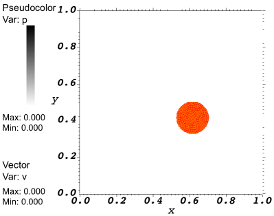
(a) $t={\numprint[s]{0}}$

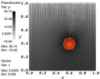
(b) $t={\numprint[s]{0.01}}$

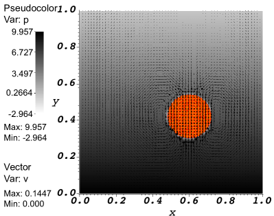
(c) $t={\numprint[s]{0.5}}$

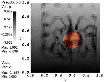
(d) $t={\numprint[s]{1.0}}$

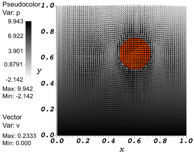
(e) $t={\numprint[s]{2.0}}$

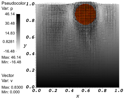
(f) $t={\numprint[s]{3.0}}$

Figure 3: The velocity field over the entire control volume, the pressure in the fluid and the mesh of the disk.

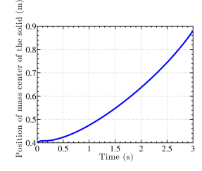
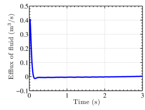
Figure 4: Instantaneous vertical position of the disk and flux of the fluid.

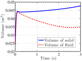
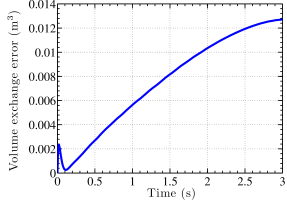
Figure 5: Instantaneous area change of the disk, amount of fluid ejected from the control volume and the difference between them as an estimate of the error in our numerical implementation.

5.2 Deformation of a compressible annulus under the action of point source of fluid

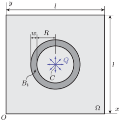
Figure 6: Initial configuration of an annulus immersed in a square box filled with fluid. At the center $C$ of the box there is a point source of strength $Q$.

This test was first proposed by Roy Roy-2012-a , as a toy model to describe the behavior of hydrocephalus in the brain. In this test we observe the deformation of a hollow cylinder, submerged in a fluid contained in a rigid prismatic box, due to the influx of fluid along the axis of the cylinder. In the two-dimensional context the test comprises an annular solid with inner radius $R$ and thickness $w$ that is concentric with a fluid-filled square box of edge length $l$ (see, Fig. 6). A point mass source of fluid of strength $Q$ is located at $\mathbf{x}_{C}$ which corresponds to the center $C$ of the control volume. The radially symmetric nature of point source ensures that momentum balance law remains unaltered. However, we need to modify the balance of mass to account for the mass influx from the point source by adding the following term to the pressure equation:

$$\dfrac{Q}{\rho_{\mathbf{f}}}\delta\left(\mathbf{x}-\mathbf{x}_{C}\right)$$ (34)

For this test we have used a single point source whose strength is a constant, and all boundary conditions on the control volume are of homogeneous Dirichlet type.The solid is compressible and hence volume of solid and thereby the volume of fluid in the control volume can change. The homogeneous Dirichlet boundary condition implies that the fluid cannot leave the control volume and hence the amount of fluid that accumulates in the control volume due to the point source must equate the decrease in volume of the solid. The difference in these two volumes can serve as an estimate of the numerical error incurred.

Table 1: Number of cells and DoFs used in the different simulations involving the deformation of a compressible annulus under the action of a point source.

	Solid		Control Volume
	Cells	DoFs	Cells	DoFs
Level 1	6240	50960	1024	9539
Level 2	24960	201760	4096	37507
Level 3	99840	802880	16384	148739

We have used the following parameters for this test: $R=\numprint[m]{0.25}$, $w=\numprint[m]{0.05}$, $l=\numprint[m]{1.0}$, $\rho_{\mathbf{f}}=\rho_{\mathbf{s}_{0}}=\numprint[kg/m^{3}]{1}$, $\mu_{\mathbf{f}}=\mu_{\mathbf{s}}=\numprint[Pa\!\cdot\!s]{1}$, $\mu^{e}=\numprint[Pa]{1}$, $\nu=0.3$, $Q=\numprint[kg/s]{0.1}$ and $dt=\numprint[s]{0.01}$. We have tested for three different mesh refinement levels whose details have been listed in Table 1.

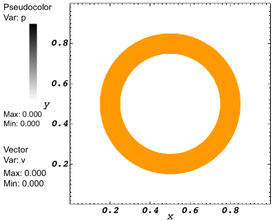
(a) $t={\numprint[s]{0}}$

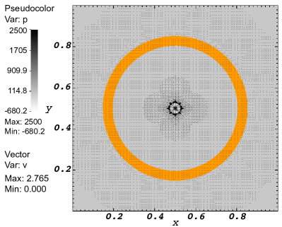
(b) $t={\numprint[s]{1.0}}$

Figure 7: The velocity and the mean normal stress field over the control volume. Also shown is the annulus mesh.

The initial state of the system is shown in Fig. 7(a). As time progresses, the fluid entering the control volume deforms and compresses the annulus as shown in Fig. 7(b) for $t=\numprint[s]{1}$. When we look at the difference in the instantaneous amount of fluid entering the control volume and the decrease in the volume of the solid, we see that the difference increases over time (see Fig. 8). This is not surprising since the mesh of the solid becomes progressively distorted as the fluid emanating from the point source push the inner boundary of the annulus. The error significantly reduces with the increase in the refinements of the fluid and the solid meshes.

Figure 8: The difference between the instantaneous amount of fluid entering due to the source and the change in the area of the annulus. The difference reduces with mesh refinement.

6 Conclusions

The Finite Element Immersed Boundary Method (FEIBM) is a well established formulation for fluid structure interaction problems of general types. In most implementations (see, for example,  BoffiGastaldiHeltaiPeskin-2008-a ), the solid constitutive behavior is constrained to be viscous (with the same viscosity of the surrounding fluid) and incompressible.

The first attempt to allow for solids of arbitrary constitutive type was presented in HeltaiCostanzo-2012-a , whose formulation is applicable to problems with immersed bodies of general topological and constitutive characteristics. Such formulation, however, did not expose the intrinsic structure of the underlying problem.

In this work we have shows how the incompressible version of the FSI model presented in HeltaiCostanzo-2012-a can be seen as a special case of the Distributed Lagrange Multiplier method, introduced in BoffiCavalliniGastaldi-2015-a , and we presented a novel distributed Lagrange multiplier method that generalizes the compressible model introduced in HeltaiCostanzo-2012-a .

Two validation tests are presented, to demonstrate the capability of the model to take into account complex fluid structure interaction problems between compressible solids and incompressible fluids.

References

- [1] D. Arndt, W. Bangerth, D. Davydov, T. Heister, L. Heltai, M. Kronbichler, M. Maier, J.-P. Pelteret, B. Turcksin, and D. Wells. The deal.II library, version 8.5. Journal of Numerical Mathematics, 25(3), jan 2017.
- [2] D. Boffi, N. Cavallini, F. Gardini, and L. Gastaldi. Local mass conservation of Stokes finite elements. J. Sci. Comput., 52(2):383–400, 2012.
- [3] D. Boffi, N. Cavallini, and L. Gastaldi. The finite element immersed boundary method with distributed Lagrange multiplier. SIAM Journal on Numerical Analysis, 53(6):2584–2604, 2015.
- [4] D. Boffi and L. Gastaldi. A finite element approach for the immersed boundary method. Computers & Structures, 81(8–11):491–501, 2003.
- [5] D. Boffi, L. Gastaldi, L. Heltai, and C. S. Peskin. On the hyper-elastic formulation of the immersed boundary method. Computer Methods in Applied Mathematics and Engineering, 197(25–28):2210–2231, 2008.
- [6] M. E. Gurtin. An introduction to continuum mechanics, volume 158. Academic press, 1982.
- [7] L. Heltai and F. Costanzo. Variational implementation of immersed finite element methods. Comput. Methods Appl. Mech. Engrg., 229/232:110–127, 2012.
- [8] L. Heltai, S. Roy, and F. Costanzo. A fully coupled immersed finite element method for fluid structure interaction via the Deal.II library. Archive of Numerical Software, 2(1), 2014.
- [9] T. J. R. Hughes, W. K. Liu, and Zimmerman T. K. Lagrangian-Eulerian finite element formulations for incompressible viscous flows. Computer Methods in Applied Mechanics and Engineering, 29:329–349, 1981.
- [10] C. S. Peskin. Numerical analysis of blood flow in the heart. Journal of Computational Physics, 25(3):220–252, 1977.
- [11] C. S. Peskin. The immersed boundary method. Acta Numerica, 11:479–517, 2002.
- [12] Saswati Roy. Numerical simulation using the generalized immersed finite element method: an application to hydrocephalus. PhD thesis, The Pennsylvania State University, 2012.
- [13] Saswati Roy, Luca Heltai, and Francesco Costanzo. Benchmarking the immersed finite element method for fluid-structure interaction problems. Computers and Mathematics with Applications, 69:1167–1188, 2015.
- [14] S. Turek and J. Hron. Proposal for numerical benchmarking of fluid-structure interaction between an elastic object and laminar incompressible flow. In H.-J. Bungartz and M. Schäfer, editors, Fluid-Structure Interaction, volume 53 of Lecture Notes in Computational Science and Engineering, pages 371–385. Springer, Berlin, Heidelberg, 2006. DOI: 10.1007/3-540-34596-5_15.
- [15] X. Wang and W. K. Liu. Extended immersed boundary method using FEM and RKPM. Computer Methods in Applied Mechanics and Engineering, 193(12–14):1305–1321, 2004.
- [16] L. Zhang, A. Gerstenberger, X. Wang, and W. K. Liu. Immersed finite element method. Computer Methods in Applied Mechanics and Engineering, 193(21–22):2051–2067, 2004.