Tomographic reconstruction using
global statistical priors

Abstract

Recent research in tomographic reconstruction is motivated by the need to efficiently recover detailed anatomy from limited measurements. One of the ways to compensate for the increasingly sparse sets of measurements is to exploit the information from templates, i.e., prior data available in the form of already reconstructed, structurally similar images. Towards this, previous work has exploited using a set of global and patch based dictionary priors. In this paper, we propose a global prior to improve both the speed and quality of tomographic reconstruction within a Compressive Sensing framework.

We choose a set of potential representative 2D images referred to as templates, to build an eigenspace; this is subsequently used to guide the iterative reconstruction of a similar slice from sparse acquisition data. Our experiments across a diverse range of datasets show that reconstruction using an appropriate global prior, apart from being faster, gives a much lower reconstruction error when compared to the state of the art.

I Introduction

Improvements in tomographic reconstruction from sparse measurements are being widely sought after, due to their benefit of aiding lower exposure to the ionizing X-rays. However, the quality of reconstruction is directly limited by the number of measurements captured. When sampling is below the Nyquist limit, the data cannot be uniquely reconstructed by direct inversion methods. Hence, given an exceedingly smaller number of measurements, the reconstruction must rely on some known information about the data for better reconstruction fidelity. This information compensates for the sub-Nyquist sampling of the data. The information could be, for example, the sparsity of the data under some transform. Compressive sensing (CS) [1] routines exploit this information to recover the sparse coefficients of the underlying data, with proven guarantees for error bounds.

Our previous work [2] partitioned a volume comprised of consecutive 2D slices into local groups of slices before performing the reconstruction of this volume from a sparse set of projected views. The grouping of these slices was based on their structural similarity, as measured through a comparison of the invariant moments of their projected views. Acquiring local knowledge of the object structure enabled significant improvement, as now the CS reconstruction could be performed on groups of similar slices that were able to be reconstructed much better than the individual, slice by slice CS reconstructions. In addition to this, recent research has also focussed on using known information that is specific to the type of data being measured, for example, an existing similar data, also known as the prior. Such a technique has been referred to as Prior Image Constrained Compressed Sensing (PICCS) [3]. Here, the similarity between the prior and the reconstructed data is explicitly enforced in the iterative routines. This offers further reduction in sampling when compared to plain CS, for a desired reconstruction quality.

However, in scenarios where the similarity of the prior and test data are not guaranteed, the application of PICCS will hurt the reconstruction. Moreover, selecting any one particular optimal slice or volume as a prior from a huge amount of available data, can be challenging. To evade this shortcoming, a large amount of work has been done on the usage of a set of slices or volumes as prior data [4], [5], [6], [7], [8]. The similarity of the test slice to any one of the templates is then more probable. One application scenario for using a prior is in the case of long-term treatments, in which a subject might undergo CT scan multiple times. The subsequent scans can then be taken with fewer projections by exploiting the information available from all or a few of the previous good quality scans.

Contributions: In this work, we develop on the idea of using multiple templates by hypothesizing that the test slice may not be exactly similar to any of the slices in the template set, but lies in the subspace spanned by the templates. In such a case, the test slice can be expressed as a linear combination of the principal components of the template slices. Hence, we form an eigenspace from a set of template slices and use this as our prior data. We have compared our results with plain CS, filtered back-projection and patch based dictionary methods and observed a substantial improvement with highly undersampled and noisy measurements.

In Section II, we discuss the existing literature in prior-based reconstructions. In Section III, we describe the proposed global-prior-based technique, followed by the patch based dictionary technique in Section IV. The results of our experiments on five CT datasets are described in Section V, followed by some conclusions, and future work in Section VI.

II Previous work

The quality of image reconstruction depends on the type of recovery algorithm used and the way in which the prior is used. Among the various types of iterative recovery algorithms, Compressed Sensing (CS) [1] is being widely used in tomographic reconstruction due to its theoretical guarantee [9] of powerful data recovery from noisy sub-Nyquist measurements.

Among the prior aided methods, a direct extension of the PICCS based method is the usage of multiple priors. This is demonstrated in [10], where the optimal weights to the set of priors is adaptively tuned after each iteration of reconstruction. Many methods have also been proposed recently to exploit local prior data. In [4], volume reconstruction from low dose CT was performed using a 3D patch based overcomplete dictionary built offline from a set of good quality scan volumes. The performance of this dictionary was shown to be superior to Simultaneous Iterative Reconstruction Technique (SIRT), 3D-TV and 2D slice-wise patch based dictionary. There has also been previous work based on the update of the 2D patch based dictionary during the reconstruction process, based on the intermediate reconstructions [5]. This is however computationally very expensive. In [6], dual dictionaries have been built for 3D MRI volume reconstruction, one corresponding to low resolution volume and other for high resolution volume. In this way, the similarity between the volumes with different resolutions is exploited. Since this dual-dictionary is fixed and sensitive to parameters of reconstruction, an adaptive dual dictionary was built in [7]. The adaptive version was performed on 2D patches. In  [8], both the MRI sampling position and the weight given to the prior are varied in real-time based on the differences between a single template volume and the test volume. Instead of using a set of templates, [11] had used one template image and its patches were classified into multiple classes based on their geometrical orientation. A separate dictionary was then learned on each class of patch. The intermediate reconstructions were used to update the template slice and the whole process was repeated.

In contrast to all the previous work, we propose to use a more accurate and faster global Principal Component Analysis (PCA) based dictionary as part of the CS scheme.

(a)

(b)

Figure 1: Data from walnut CT dataset [12]. Each slice is of size $260\times 260$. (a) Seven templates (slice nos. 70, 80, 90, 100, 110, 120 and 130 from the CT volume) that were used to build the prior. (b) The test data (slice no. 105 from the same volume).

(a)

(b)

Figure 2: Offline tuning for $\lambda_{2}$ for the use of global PCA based prior in the walnut CT dataset [12] to reconstruct the test slice shown in figure 1(b). (a) reconstruction for $\lambda_{2}$ varying from $0$ to $2$ ins-eps-converted-to.pdf of $0.1$ (b) variation in relative mean squared error for different values of $\lambda_{2}$.

III Computing global statistical prior

We begin with the assumption that the test slice can be expressed as a compact linear combination of the principal components extracted from a set of similar slices (called here as ‘templates’). Hence, we build the prior using PCA, which has been a widely used technique to represent data in terms of its significant modes or directions of variation.

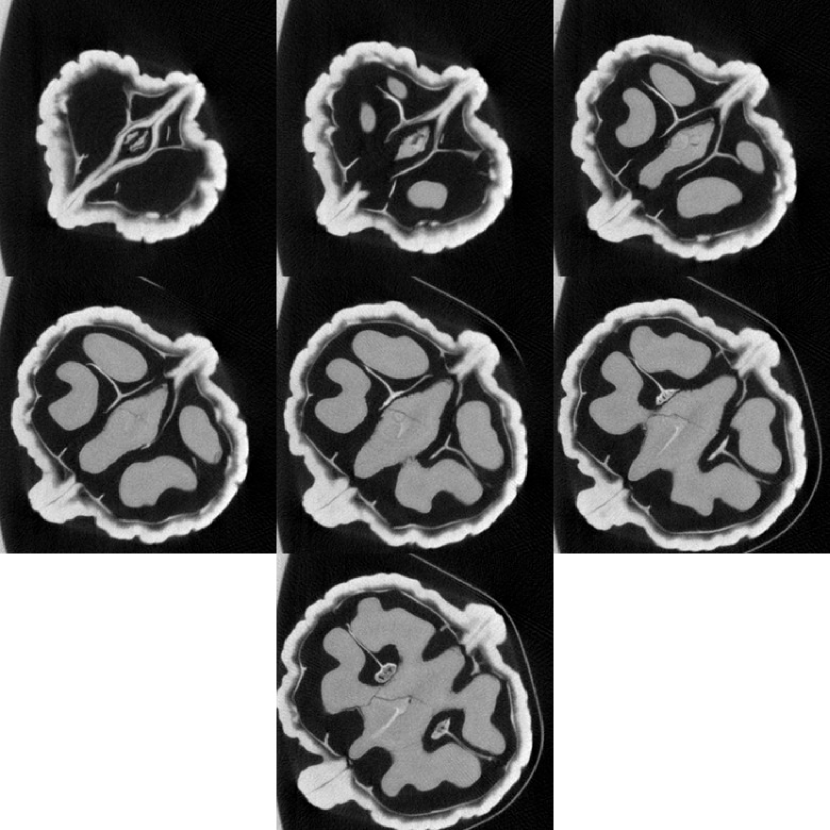
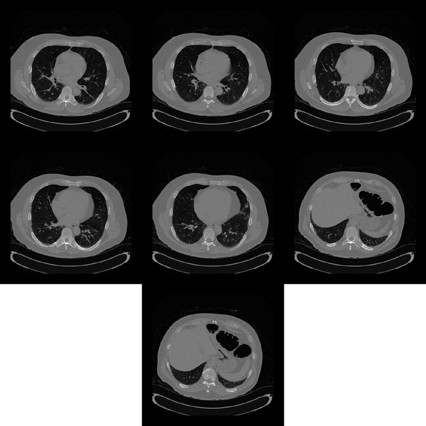
In our algorithm, we choose a set of representative 2D slices as templates. These templates must represent a wide range of anatomy in order to contribute to an eigenspace that can encompass a range of possible test slice anatomy. If these slices are from different volumes, then they must be first registered before computing the prior. The prior is built by computing the covariance matrix $C$ from the template set $\{t_{i}\}$, as shown in Eq. 1, The space spanned by the eigenvectors $\{V_{i}\}$ (eigenspace) of the covariance matrix is our global prior and is assumed to contain any test slice that is similar, but not necessarily identical to the templates.

The covariance matrix is given by:

$$\begin{split}C&=\frac{1}{N-1}\sum_{i=1}^{N}(t_{i}-\mu)(t_{i}-\mu)^{T}\\ \end{split}$$ (1)

where $\mu$ denotes the mean of all templates $\{t_{i}\}$ and $N$ denotes the number of templates chosen.

Once the prior eigenspace is learned offline, the reconstruction is performed iteratively by minimizing an objective function. This minimization is done using the Compressive Sensing (CS) based routines. Let $\Phi$ denote the Radon measurement matrix under a chosen set of angles, $\theta$ denote the sparse 2D-DCT (Discrete Cosine Transform) coefficients of the slice to be reconstructed, and $\Psi$ denote the inverse DCT basis matrix. The DCT is commonly used to sparsely represent naturally occurring images in the CS framework. The objective function to be minimized in the plain CS technique is given by:

$$E(\mathbf{\theta})=||\Phi\Psi\mathbf{\theta}-y||_{2}^{2}+\lambda_{1}||\mathbf{\theta}||_{1}$$ (2)

After inclusion of the PCA based prior, this objective function $E$ is given by :

$$E(\mathbf{\theta},\mathbf{\alpha})=||\Phi\Psi\mathbf{\theta}-y||_{2}^{2}+\lambda_{1}||\mathbf{\theta}||_{1}+\lambda_{2}||\Psi\mathbf{\theta}-(\mu+\sum_{i}V_{i}\alpha_{i})||_{2}^{2}$$ (3)

where $V_{i}$ denotes the $i^{th}$ principal component or eigenvector and $\alpha$ denotes the eigen coefficients of $\Psi\mathbf{\theta}$ (an estimate of the underlying test slice). We solve for $\theta$ and $\alpha$ by alternately minimizing Eq. 4 by assuming a fixed $\alpha$, and Eq. 6, by using a fixed $\mathbf{\theta}$. Eq. 4 is solved using the $l1\_ls$ solver [13], one of the popular solvers used in the literature.

$$E_{\mathbf{\alpha}}(\mathbf{\theta})=||\Phi\Psi\mathbf{\theta}-y||_{2}^{2}+\lambda_{1}||\mathbf{\theta}||_{1}+\lambda_{2}||\Psi\mathbf{\theta}-(\mu+\sum_{i}V_{i}\alpha_{i})||_{2}^{2}$$ (4)

$$E_{\mathbf{\theta}}(\alpha)=||\Psi\mathbf{\theta}-(\mu+\sum_{i}V_{i}\alpha_{i})||_{2}^{2}$$ (5)

Eq. 5 leads to the following closed form update for $\alpha$:

$$\mathbf{\mathbf{\alpha}}=\mathbf{V}^{T}(\Psi\mathbf{\theta}-\mu)$$ (6)

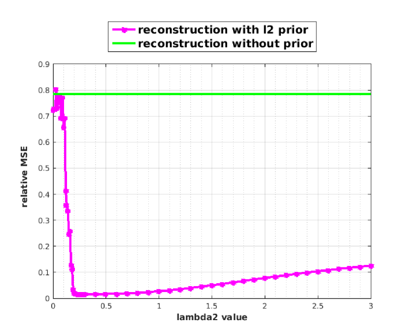
An optimal value of $\lambda_{2}$ is empirically chosen a priori, based on the reconstructions of one of the template slices. The variation in relative mse (relative mean squared error) for different weights of the template based prior, $\lambda_{2}$ is shown in figure 2.

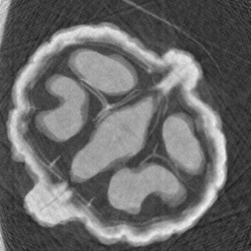
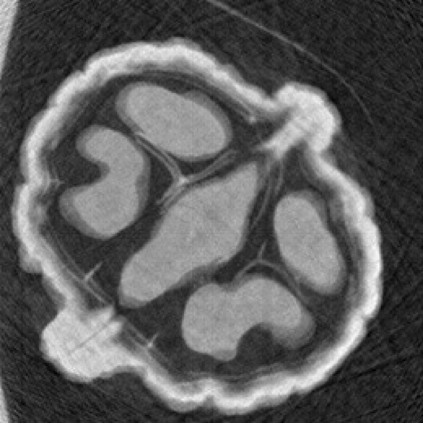
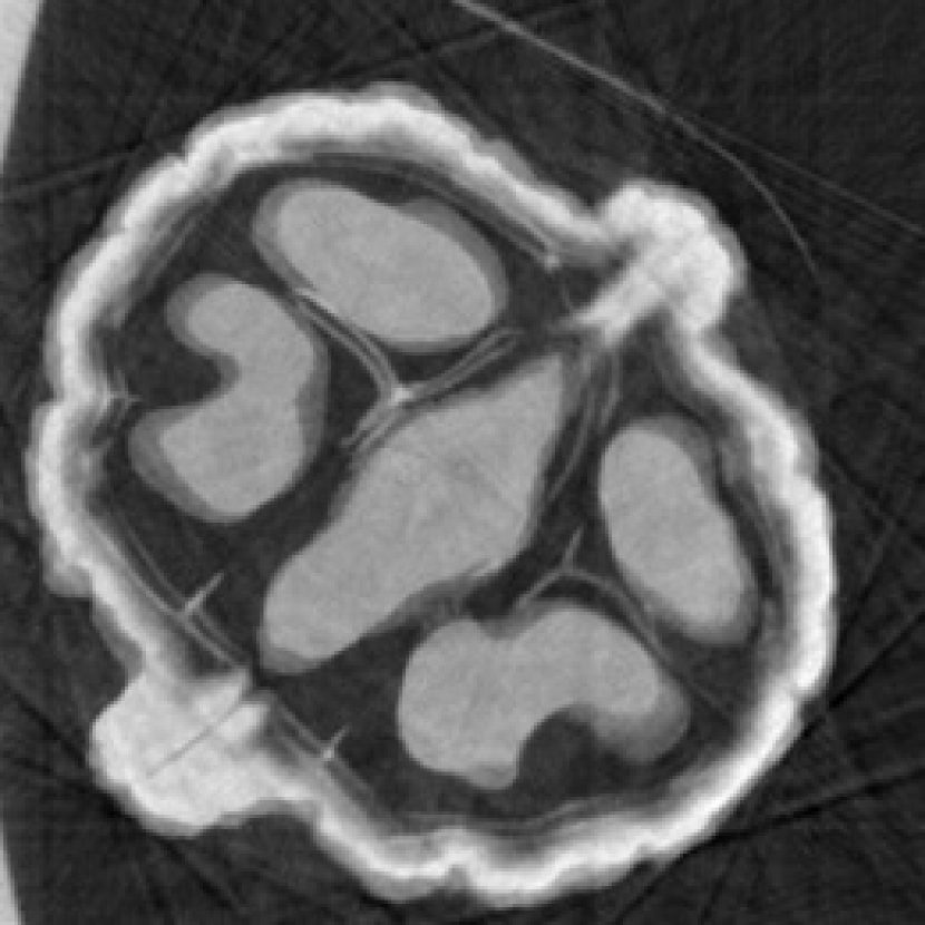
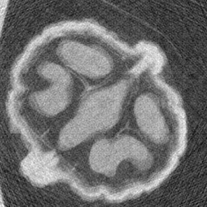
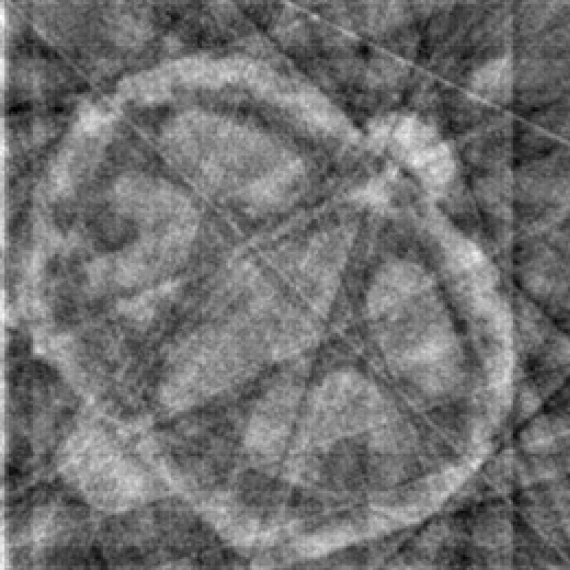
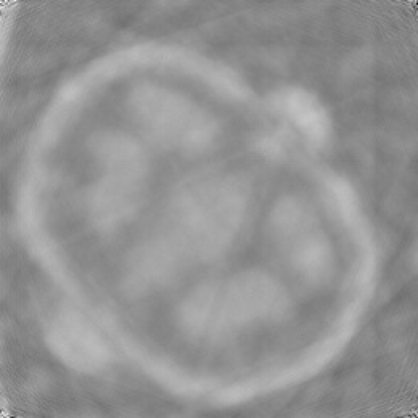
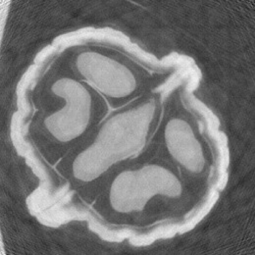
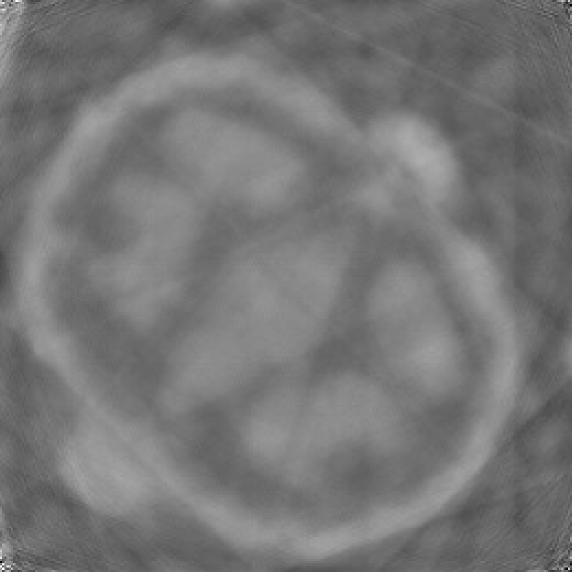
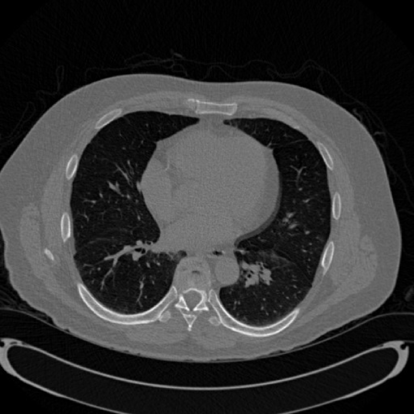
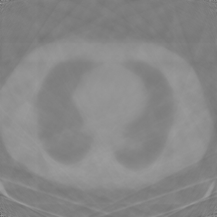
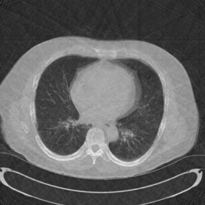
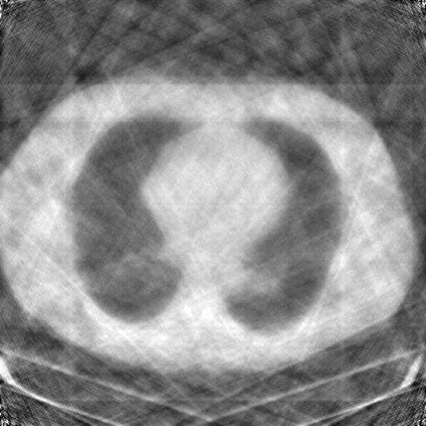
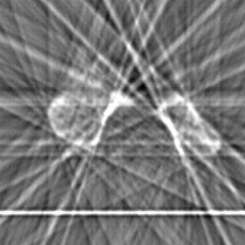
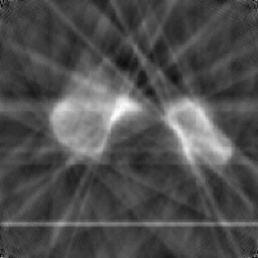
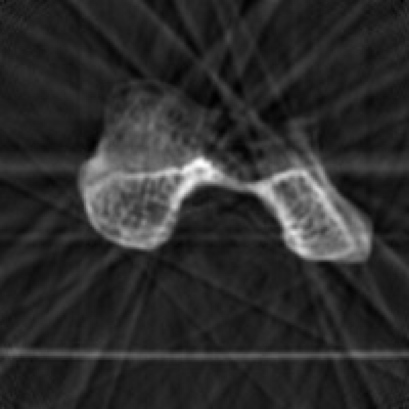
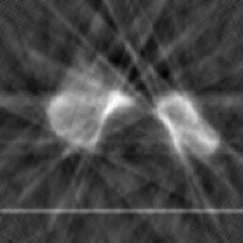
Figures  3 and 4 show the results of PCA based reconstruction for different measurement angles and different levels of noise, after tuning for the optimal $\lambda_{1}$ and $\lambda_{2}$.

(a)

(b)

(c)

(d)

(e)

(f)

(g)

(h)

Figure 3: Reconstructions using the global PCA based prior for various measurement angles: (a) 8 angles (b) 10 angles (c) 12 angles (d) 14 angles (e) 16 angles (f) 20 angles (g) 30 angles (h) 40 angles. $2\%$ Gaussian iid noise was added to the measurements in all the cases.

TABLE I: Performance of the global PCA based reconstruction for various measurement angles, corresponding to the results shown in figure 3

No. of angles (uniformly distributed)	relative mse	ssim
8	0.0389	0.3113
10	0.0379	0.3165
12	0.0370	0.3097
14	0.0366	0.3111
16	0.0347	0.3163
20	0.0330	0.3248
30	0.0300	0.3351
40	0.0275	0.3472

(a)

(b)

(c)

Figure 4: Performance of the global PCA based reconstruction for different noise levels (measurements for 12 angles): (a) no noise (relative mean squared error (relative mse) = 0.0331, ssim = 0.3475), (b) $2\%$ noise (relative mse = 0.0370, ssim = 0.3097) (h) $10\%$ noise (relative mse = 0.0697, ssim = 0.2191).

(a)

(b)

(c)

(d)

Figure 5: Reconstruction of a slice from the walnut CT dataset [12] from measurements along 12 angles and with 2% noise. (a) Reconstructed by filtered backprojection (b) Reconstructed slice using plain CS, without any prior (c) Reconstructed slice using CS, with global prior (d) Reconstructed slice using CS, with patch based prior with patch size = $13\times 13$ pixels.

(a)

(b)

Figure 6: Data from colon CT dataset [14]. Each slice is of size $512\times 512$. (a) Seven templates (slice nos. 13, 23, 33, 43, 53, 63 and 73 from the CT volume) that were used to build the prior. (b) The test data (slice no. 38 from the same volume).

(a)

(b)

(c)

(d)

Figure 7: Reconstruction of a slice from the colon CT dataset [14] from measurements along 15 angles and with 2% noise. (a) Reconstructed by filtered backprojection (b) Reconstructed slice using plain CS, without any prior (c) Reconstructed slice using CS, with global prior (d) Reconstructed slice using CS, with patch based prior with patch size = $8\times 8$ pixels.

(a)

(b)

Figure 8: Data from humerus CT dataset [15]. Each slice is of size $200\times 200$. (a) Six templates (slice nos. 55, 65, 75, 85, 95 and 105 from the CT volume) that were used to build the prior. (b) The test data (slice no. 70 from the same volume).

(a)

(b)

(c)

(d)

Figure 9: Reconstruction of a slice from the humerus bone CT dataset [15] from measurements along 10 angles and with 2% noise. (a) Reconstructed by filtered backprojection (b) Reconstructed slice using plain CS, without any prior (c) Reconstructed slice using CS, with global prior (d) Reconstructed slice using CS, with patch based prior with patch size = $8\times 8$ pixels.

(a)

(b)

Figure 10: Data from pelvis CT dataset [16]. Each slice is of size $512\times 512$. (a) Five templates (slice nos. 50, 60, 70, 80 and 90 from the CT volume) that were used to build the prior. (b) The test data (slice no. 95 from the same volume).

(a)

(b)

(c)

(d)

Figure 11: Reconstruction of a slice from the pelvis CT dataset [16] from measurements along 18 angles and with 2% noise. (a) Reconstructed by filtered backprojection (b) Reconstructed slice using plain CS, without any prior (c) Reconstructed slice using CS, with global prior (d) Reconstructed slice using CS, with patch based prior with patch size = $8\times 8$ pixels.

(a)

(b)

Figure 12: Data from shoulder CT dataset [17]. Each slice is of size $512\times 512$. (a) Six templates (slice nos. 350, 360, 370, 380, 390 and 400 from the CT volume) that were used to build the prior. (b) The test data (slice no. 385 from the same volume).

(a)

(b)

(c)

(d)

Figure 13: Reconstruction of a slice from the shoulder CT dataset [17] from measurements along 16 angles and with 2% noise. (a) Reconstructed by filtered backprojection (b) Reconstructed slice using plain CS, without any prior (c) Reconstructed slice using CS, with global prior (d) Reconstructed slice using CS, with patch based prior with patch size = $8\times 8$ pixels.

IV Comparison with Patch based techniques

We have compared the performance of the proposed PCA based global prior with the patch based dictionary prior, both using CS recovery routines. To build the patch based dictionary, we use the K-SVD algorithm. The template slices are divided into patches and an overcomplete dictionary is learned using the extracted patches. The K-SVD algorithm aims to sparsely represent all the patches using the dictionary. Once this dictionary is computed offline, the reconstruction of a new test slice is performed by minimizing the following objective function:

$$E(\mathbf{\theta},\mathbf{\alpha})=||\Phi\Psi\mathbf{\theta}-y||_{2}^{2}+\lambda_{1}||\mathbf{\theta}||_{1}+\frac{\lambda_{2}}{N_{p}}\sum_{i=1}^{N_{p}}||P_{i}\Psi\mathbf{\theta}-D\alpha_{i}||_{2}^{2}\\ +\frac{\lambda_{3}}{N_{p}}\sum_{i=1}^{N_{p}}||\mathbf{\alpha_{i}}||_{1}$$ (7)

where D is the dictionary learned, $N_{p}$ is the total number of patches and $P_{i}$ is the operator to extract the $i^{th}$ patch from the intermediate reconstructed slice. The reconstruction is performed by alternate minimization of Eq 8 and Eq. 9, both using $l1\_ls$ solver.

$$E_{\mathbf{\alpha}}(\mathbf{\theta})=||\Phi\Psi\mathbf{\theta}-y||_{2}^{2}+\lambda_{1}||\mathbf{\theta}||_{1}+\frac{\lambda_{2}}{N_{p}}\sum_{i=1}^{N_{p}}||P_{i}\Psi\mathbf{\theta}-D\alpha_{i}||_{2}^{2}$$ (8)

For each $i=1..N_{p}$,

$$E_{\mathbf{\theta}}(\mathbf{\alpha}_{i})=||P_{i}\Psi\mathbf{\theta}-D\alpha_{i}||_{2}^{2}+\frac{\lambda_{3}}{\lambda_{2}}||\mathbf{\alpha_{i}}||_{1}$$ (9)

This method requires prior tuning of three parameters: $\lambda_{1},\lambda_{2}$ and $\lambda_{3}$. This is done by reconstructing one of the template slices a priori.

V Experiments and Results

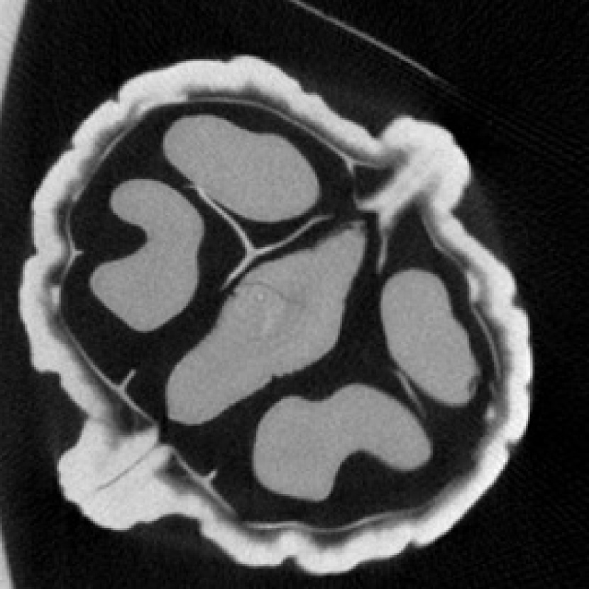
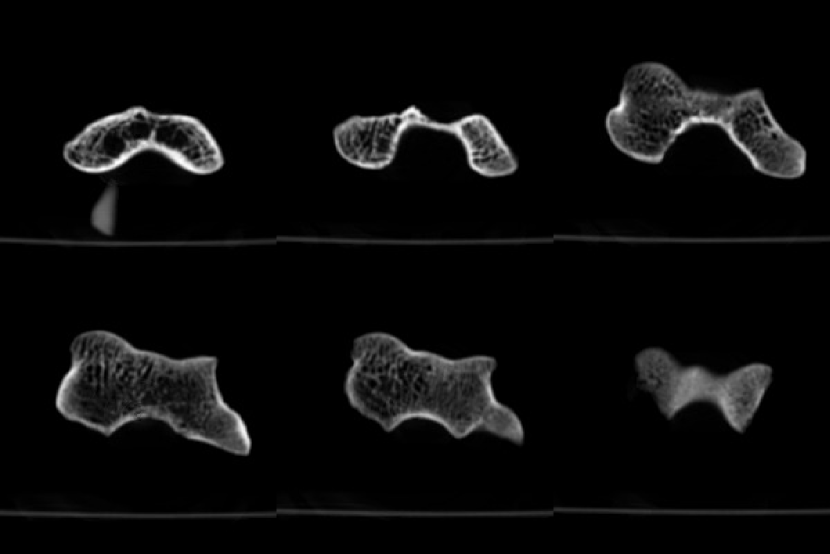
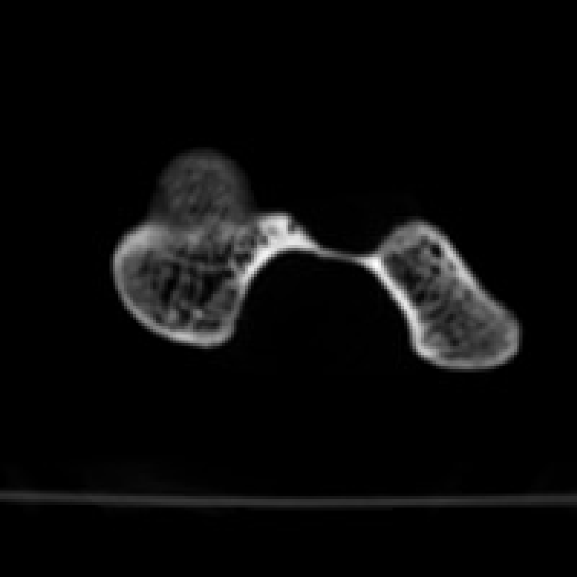
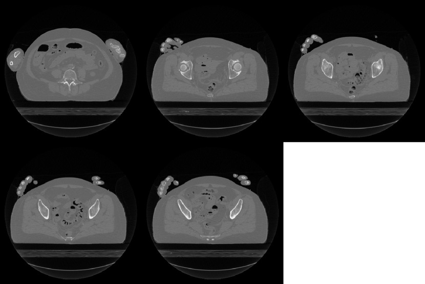
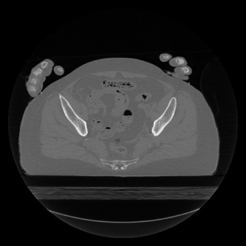
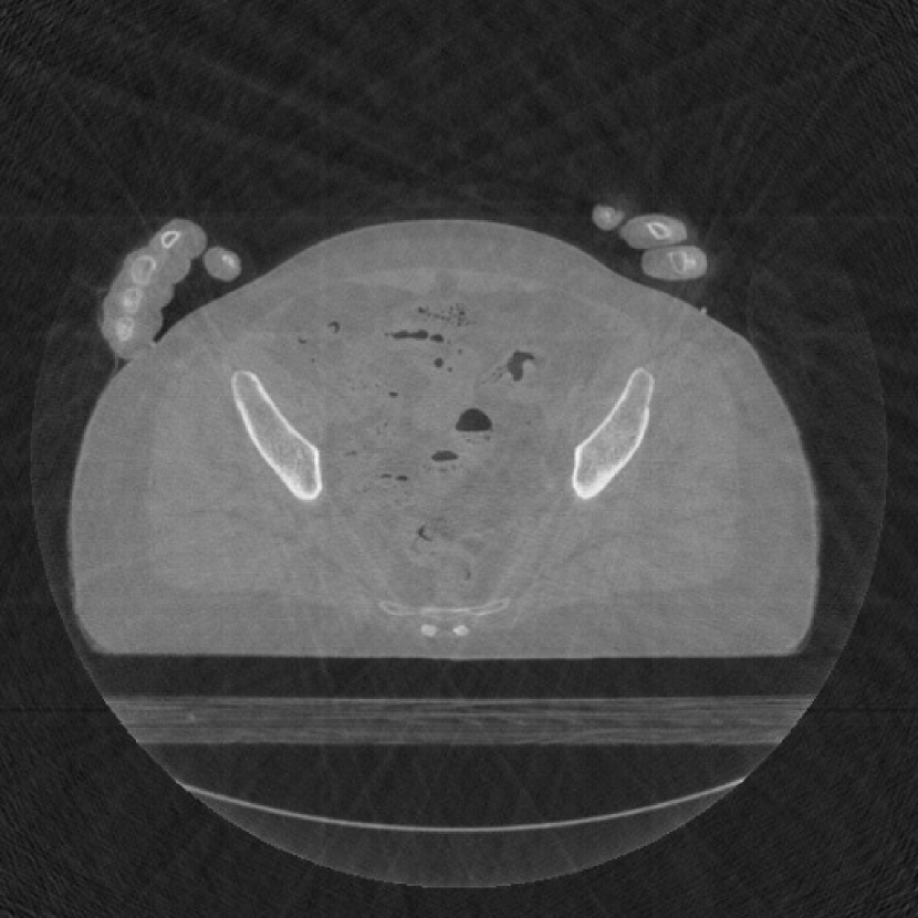
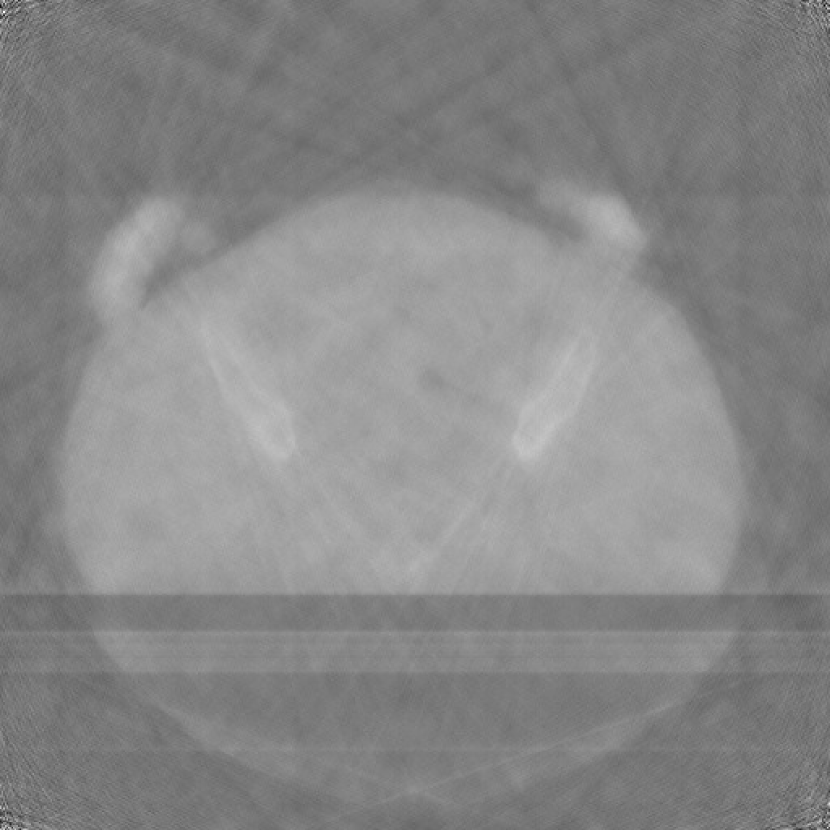
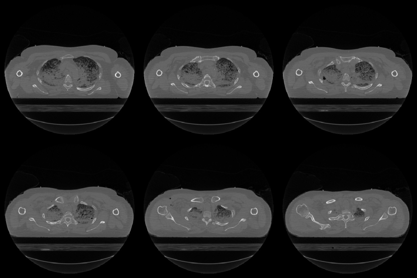
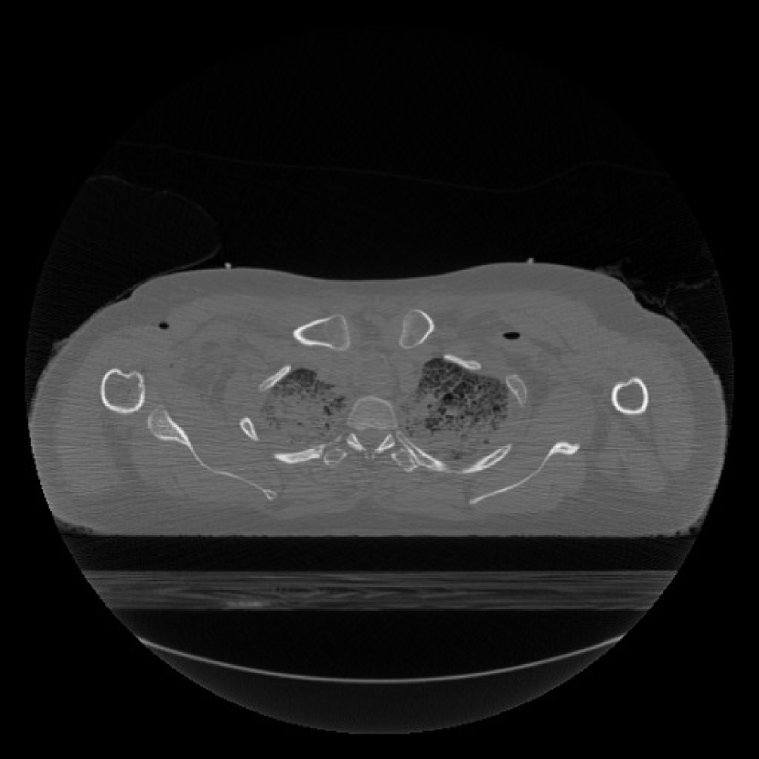
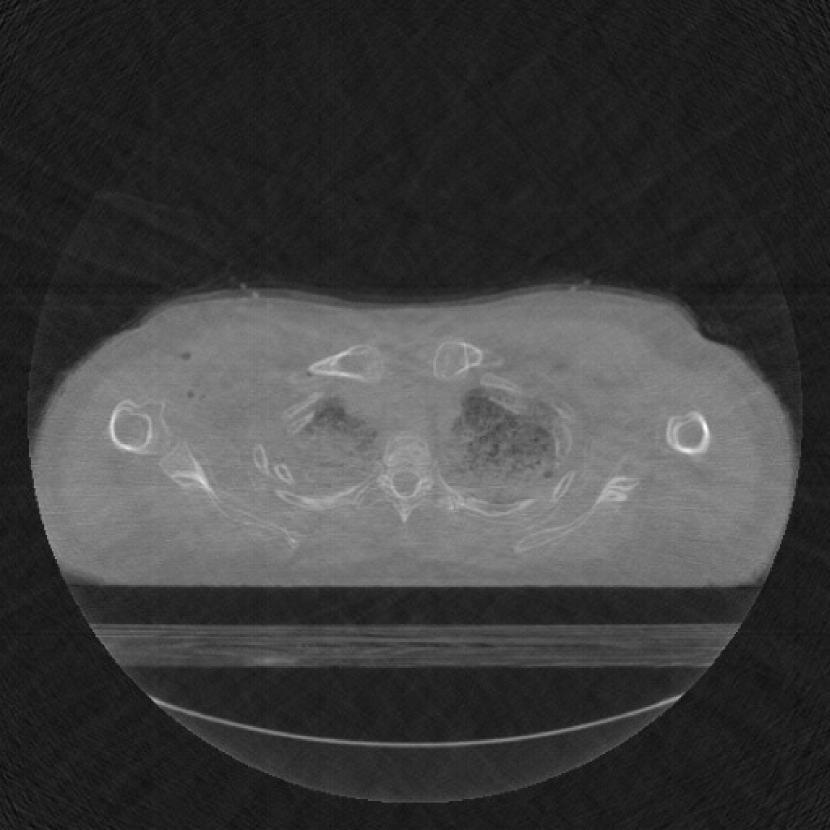
We have built the template set using 5-7 slices from a volume of each dataset. Using more slices may not necessarily help if a subset is sufficient to represent all the variations that the test slice could possess. The chosen test slices are similar to, but not identical to any of the template slices. However, in our experiments so far, the templates and test slices have been chosen from the same volume. Figures 1(a), 6(a), 8(a), 10(a) and 12(a) show the chosen template sets for each of the five datasets and figures 1(b), 6(b), 8(b), 10(b) and 12(b) show the corresponding test slices. To build the patch based dictionary, we have chosen patch size of $8\times 8$ for the pelvis, colon, shoulder and humerus datasets and patch size of $13\times 13$ for walnut dataset. In all the datasets, iid Gaussian noise with standard deviation equal to $2\%$ of mean of the projections was added to the measurements before reconstruction.

The global PCA based method has been compared with the following methods: a) filtered backprojection (using ‘Cosine’ filter), b) plain CS technique that uses only sparsity of DCT prior (i.e. with $\lambda_{2}$ and $\lambda_{3}$ set to 0); and c) plain CS DCT prior + patch based dictionary. The visual reconstruction results are shown in figures 5, 7, 9, 11 and 13, and the relative mse and the Structural SIMilarity (ssim) index of the results are shown in tables II, III, IV, V and  VI.

Relative mse refers to the relative mean squared error and is given by $(1/n)(\sum_{i}(y_{i}-x_{i})^{2}/\sum_{i}(x_{i})^{2})$ where $n$ refers to the number of pixels. SSIM [18] is a better evaluation metric that computes the similarity in shape and structure of the contents of one image to that of the other.

It is evident that the PCA based prior (coupled within the CS framework) works best. The patch based dictionary doesn’t contribute much to the further improvement over plain CS technique. In previous work, the performance of the patch based dictionaries has not been compared with plain CS reconstruction, as has been done here.

All experiments were performed on MATLAB on a 14-core Xeon CPU with a processor at 2.6GHz and RAM of 32GB. Table VII shows the approximate time taken for training and reconstruction phases for experiments on a $260\times 260$ sized slice from measurements along 12 angles and with $2\%$ noise. Computationally, the global prior based method is much faster than the patch based dictionary method during both the offline prior generation process and the online reconstruction process.

TABLE II: Performance of reconstruction in walnut dataset.

Method	relative mse	ssim
Filtered backprojection	0.4580	0.1447
Plain Compressive Sensing	0.7724	0.0230
Patch based dictionary prior	0.8511	0.0103
Global PCA based prior	0.0172	0.5150

TABLE III: Performance of reconstruction in colon dataset.

Method	relative mse	ssim
Filtered backprojection	0.5844	0.0505
Plain Compressive Sensing	0.5266	0.0261
Patch based dictionary prior	0.7951	0.0192
Global PCA based prior	0.0280	0.1783

TABLE IV: Performance of reconstruction in humerus dataset.

Method	relative mse	ssim
Filtered backprojection	1.4089	0.0669
Plain Compressive Sensing	0.2969	0.0743
Patch based dictionary prior	0.2839	0.0777
Global PCA based prior	0.2718	0.0759

TABLE V: Performance of reconstruction in pelvis dataset.

Method	relative mse	ssim
Filtered backprojection	0.4081	0.0418
Plain Compressive Sensing	0.3131	0.0438
Patch based dictionary prior	0.0975	0.0656
Global PCA based prior	0.0274	0.1366

TABLE VI: Performance of reconstruction in shoulder dataset.

Method	relative mse	ssim
Filtered backprojection	0.4801	0.0387
Plain Compressive Sensing	0.3333	0.0428
Patch based dictionary prior	0.1154	0.0627
Global PCA based prior	0.0219	0.1389

TABLE VII: Running time comparison

	Global PCA based prior	Patch based dictionary
Training	5 sec.	3 hrs.
Testing	5 min.	20 min.

VI Conclusion and Future Work

With an aim to reconstruct data from exceedingly sparse measurements, we propose to use a PCA based global prior within a Compressed Sensing framework. We have validated our method on 2D slices of multiple, diverse datasets. When sparse measurements of $5\%-10\%$ of the full Nyquist sampling are used, our results are significantly better than the state of the art. In the future, the proposed method needs to be extended for reconstruction of test slice from different subject volumes, and for the case of three dimensional data sets.

References

- [1] D.L. Donoho, “Compressed sensing,” IEEE Transactions on Information Theory, vol. 52, no. 4, pp. 1289–1306, April 2006.
- [2] Preeti Gopal, Sharat Chandran, Imants Svalbe, and Ajit Rajwade, “Multi-slice tomographic reconstruction: To couple or not to couple,” in Proceedings of the Tenth Indian Conference on Computer Vision, Graphics and Image Processing, New York, NY, USA, 2016, ICVGIP ’16, pp. 85:1–85:7, ACM.
- [3] Guang-Hong Chen, Jie Tang, and Shuai Leng, “Prior image constrained compressed sensing (PICCS): A method to accurately reconstruct dynamic CT images from highly undersampled projection data sets,” Medical Physics, vol. 35, no. 2, pp. 660–663, 2008.
- [4] J. Liu, Y. Hu, J. Yang, Y. Chen, H. Shu, L. Luo, Q. Feng, Z. Gui, and G. Coatrieux, “3D feature constrained reconstruction for low dose CT imaging,” IEEE Transactions on Circuits and Systems for Video Technology, vol. PP, no. 99, pp. 1–1, 2016.
- [5] Q. Xu, H. Yu, X. Mou, L. Zhang, J. Hsieh, and G. Wang, “Low-dose X-ray CT reconstruction via dictionary learning,” IEEE Transactions on Medical Imaging, vol. 31, no. 9, pp. 1682–1697, Sept 2012.
- [6] Ying Song, Zhen Zhu, Yang Lu, Qiegen Liu, and Jun Zhao, “Reconstruction of magnetic resonance imaging by three-dimensional dual-dictionary learning,” Magnetic Resonance in Medicine, vol. 71, no. 3, pp. 1285–1298, 2014.
- [7] Jiansen Li, Ying Song, Zhen Zhu, and Jun Zhao, “Highly undersampled MR image reconstruction using an improved dual-dictionary learning method with self-adaptive dictionaries,” Medical & Biological Engineering & Computing, pp. 1–16, 2016.
- [8] Lior Weizman, Yonina C. Eldar, and Dafna Ben Bashat, “Compressed sensing for longitudinal MRI: An adaptive-weighted approach,” Medical Physics, vol. 42, no. 9, pp. 5195–5208, 2015.
- [9] Emmanuel J Candès, Justin Romberg, and Terence Tao, “Robust uncertainty principles: Exact signal reconstruction from highly incomplete frequency information,” Information Theory, IEEE Transactions on, vol. 52, no. 2, pp. 489–509, 2006.
- [10] H. Van Luong, J. Seiler, A. Kaup, and S. Forchhammer, “Sparse signal reconstruction with multiple side information using adaptive weights for multiview sources,” in 2016 IEEE International Conference on Image Processing (ICIP), Sept 2016, pp. 2534–2538.
- [11] Z. Zhan, J. F. Cai, D. Guo, Y. Liu, Z. Chen, and X. Qu, “Fast multiclass dictionaries learning with geometrical directions in MRI reconstruction,” IEEE Transactions on Biomedical Engineering, vol. 63, no. 9, pp. 1850–1861, Sept 2016.
- [12] “Walnut CT dataset,” https://www.uni-muenster.de/Voreen/, last viewed–April, 2017.
- [13] K. Koh, S.-J. Kim, and S. Boyd, “l1-ls: Simple matlab solver for l1-regularized least squares problems,” https://stanford.edu/~boyd/l1_ls/, last viewed–July, 2016.
- [14] “CT Colonography,” https://idash.ucsd.edu/data-collections, last viewed–April, 2017.
- [15] “Humerus CT dataset,” http://isbweb.org/data/vsj/humeral/, last viewed–July, 2016.
- [16] “Pelvis CT dataset,” https://medicine.uiowa.edu/, last viewed–June, 2017.
- [17] “Shoulder CT dataset,” https://medicine.uiowa.edu/, last viewed–June, 2017.
- [18] Zhou Wang, A. C. Bovik, H. R. Sheikh, and E. P. Simoncelli, “Image quality assessment: from error visibility to structural similarity,” IEEE Transactions on Image Processing, vol. 13, no. 4, pp. 600–612, April 2004.