Jayne Thompson
thompson.jayne2@gmail.comCentre for Quantum Technologies, National University of Singapore, 3 Science Drive 2, 117543, Singapore
Andrew J. P. Garner
Centre for Quantum Technologies, National University of Singapore, 3 Science Drive 2, 117543, Singapore
Institute for Quantum Optics and Quantum Information, Austrian Academy of Sciences, Boltzmanngasse 3, Vienna, A-1090, Austria
John R. Mahoney
Complexity Sciences Center and Physics Department,
University of California at Davis, One Shields Avenue, Davis, CA 956
James P. Crutchfield
Complexity Sciences Center and Physics Department,
University of California at Davis, One Shields Avenue, Davis, CA 956
Vlatko Vedral
Atomic and Laser Physics, University of Oxford, Clarendon Laboratory, Oxford, OX1 3PU, United Kingdom
Centre for Quantum Technologies, National University of Singapore, 3 Science Drive 2, 117543, Singapore
Department of Physics, National University of Singapore, 3 Science Drive 2, Singapore 117543
Mile Gu
gumile@ntu.edu.sgSchool of Physical and Mathematical Sciences, Nanyang Technological University, Singapore 639673, Singapore
Complexity Institute, Nanyang Technological University, Singapore 639673, Singapore
Centre for Quantum Technologies, National University of Singapore, 3 Science Drive 2, 117543, Singapore
Abstract
Causal asymmetry is one of the great surprises in predictive modelling: the memory required to predict the future differs from the memory required to retrodict the past. There is a privileged temporal direction for modelling a stochastic process where memory costs are minimal. Models operating in the other direction incur an unavoidable memory overhead. Here we show that this overhead can vanish when quantum models are allowed. Quantum models forced to run in the less natural temporal direction not only surpass their optimal classical counterparts, but also any classical model running in reverse time. This holds even when the memory overhead is unbounded, resulting in quantum models with unbounded memory advantage.
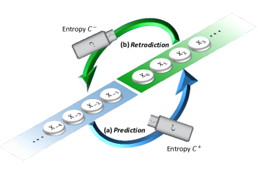
How can we observe an asymmetry in the temporal order of events when physics at the quantum level is time-symmetric? The source of time’s barbed arrow is a longstanding puzzle in foundational science Linden et al. (2009); Popescu et al. (2006); Page and Wootters (1983); Price (1997). Causal asymmetry offers a provocative perspective Crutchfield et al. (2009). It asks how Occam’s razor – the principle of assuming no more causes of natural things than are both true and sufficient to explain their appearances – can privilege one particular temporal direction over another. That is, if we want to model a process causally – such that the model makes statistically correct future predictions based only on information from the past – what is the minimum past information we must store? Are we forced to store more data if we model events in one particular temporal order over the other (see Fig. 1)?
Figure 1: A stochastic process can be modeled in either temporal order. (a) A causal model takes information available in the past
and and uses it to make statistically accurate predictions about the process’ conditional
future behaviour . (b) A retrocausal model replicates the system’s behaviour, as seen by an observer who scans the outputs from right to left encountering before . Thus it stores relevant future information , in order to generate a statistically accurate retrodiction of the past . Causal asymmetry implies a non-zero gap between the minimum memory required by any causal model , and its retrocausal counterpart .
Consider a cannonball in free fall. To model its future trajectory, we need only its current position and velocity. This remains true even when we view the process in reverse-time. This exemplifies causal symmetry. There is no difference in the amount of information we must track for prediction versus retrodiction. However this is not as obvious for more complex processes. Take a glass shattering upon impacting the floor. In one temporal direction, the future distribution of shards depends only on the glass’s current position, velocity and orientation. In
the opposite, we may need to track relevant information regarding each glass shard to infer the glass’s
prior trajectory. Does this require more or less information? This potential divergence is quantified in the theory of computational mechanics Crutchfield (2012). It is not only generally non-zero, but can also be unbounded. This phenomenon implies a simulator operating in the ‘less natural’ temporal direction is penalized with potentially unbounded memory overhead, and is cited as a candidate source of time’s barbed arrow Crutchfield et al. (2009).
These studies assumed that all models are implemented using classical physics. Could the observed causal asymmetry have been a consequence of this classicality constraint? Here, we first consider a particular stochastic process that is causally asymmetric. We determine the minimal information needed to model the same process in forward versus reverse time using quantum physics, and prove these quantities exactly coincide. More generally, we present systematic methods to model any causally asymmetric stochastic process quantum mechanically. Critically, the resulting quantum models not only use less information than any classical counterpart, but also any classical model of the time-reversed process. Thus, quantum models can field a memory advantage, that always exceeds the memory overhead incurred by causal asymmetry. Our work indicates this overhead can emerge when imposing classical causal explanations.
These result remain true even in cases where causal asymmetry becomes unbounded.
I Background
Framework – Consider a system that emits an output governed by some random variable at each discrete point in time . This behaviour can be described by a stochastic process – a joint probability distribution that correlates past behaviour, , with future expectations, . Each instance of the past exhibits a conditional future with probability .
Suppose that a model for this system can replicate this future statistical behaviour using only bits of past information. Then this model can be executed by encoding the past
into a state of a physical system of entropy , such that repeated application of a systematic action on sequentially generates , governed by the conditional future .
The model is causal if at each instance of time, all the information contains about the future can be obtained from the past 111Formally, this implies that the conditional mutual information is zero, where is the random variable governing the state of . In literature, is named oracular information, as it captures the amount of information a state of the memory stores about the future that is not contained in the past Ellison et al. (2011); Crutchfield et al. (2010). Note that this notion of causal model differs from the recent developments in quantum causal models Allen et al. (2017); Costa and Shrapnel (2016) and foundation work on causal inference Pearl (2009).. Implementing it on a computer then gives us a statistically faithful simulation of the process’
realizations. The simplest causal model for a process , is the model that minimizes .
The statistical complexity is defined as the entropy of this simplest model – it is the minimal amount of past information needed to make statistically correct future predictions Crutchfield and Young (1989); Shalizi and Crutchfield (2001). This measure is used to quantify structure in diverse settings Gonçalves et al. (1998); Park et al. (2007); Tino and Koteles (1999), including hidden variable models emulating quantum contextuality Cabello et al. (2018). also fields thermodynamic significance, having been linked to the minimal heat dissipation in stochastic simulation and the minimal structure a device needs to fully extract
free energy from non-equilibrium environments Garner et al. (2017a); Wiesner et al. (2012); Cabello et al. (2016); Boyd et al. (2017).
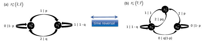
Figure 2: (a) The -machine for the process , created by a flipping a biased coin and emitting outcome when , when , and when . This process has two causal states and , where the latter includes all pasts ending in either or . (b) The time-reversed process . Here pasts ending in , and now all lead to qualitatively different future behaviour and must be stored in distinct causal states , and respectively which occur with respective probabilities , and .
Causal asymmetry captures the discrepancy in statistical complexity when a process is viewed in forward versus reverse time 222Note that in computational mechanics literature, causal asymmetry is often referred to as causal irreversibility Crutchfield et al. (2009). Here, we choose the term causal asymmetry to avoid confusion with standard notions of irreversibility used in the physics community. Consider an observer that encounters before . Their observations are characterized by the time-reversed stochastic process where past and future are interchanged, such that , while and . A causal model for the time-reversed process then corresponds to a retrocausal model for the forward process . It generates a statistically accurate retrodiction of the conditional past , using only information contained in the future . The statistical complexity of this time-reversed process (referred to as the retrodictive statistical complexity for ) quantifies the minimal amount of causal information we must assign to model in order of decreasing . Causal asymmetry captures the divergence . When , a particular temporal direction is privileged, such that modelling the process in the other temporal direction incurs a memory overhead of .
Note that the definitions above are entropic measures, and thus take operational meaning at the i.i.d. limit – i.e. modelling instances of a stochastic process with statistical complexity requires bits of past information, in the limit of large . While this is the most commonly adopted measure in computational mechanics, single shot variants do exist. The topological state complexity , is particularly noteworthy Crutchfield and Young (1989). It captures the minimum number of dimensions (max entropy) must have to generate future statistics. A single-shot variant of causal asymmetry can thus be defined by the difference , between the topological state complexities of and . Here, we focus on statistical complexity for clarity. However many of our results also hold in this single-shot regime. We return to this when relevant.
Classical models – Prior studies of causal asymmetry assumed all models were classical. In this context, causal asymmetry can be explicitly demonstrated using -machines, the provably optimal classical causal models Crutchfield and Young (1989); Shalizi and Crutchfield (2001). This involves dividing the set of pasts into equivalences classes, such that two pasts,
and lie in the same class if-and-only-if they have coinciding future behaviour, i.e., . Instead of recording the entire past, an -machine records only which equivalence class
lies within – inducing an encoding function from the space of pasts
onto the space of equivalence classes , known as
causal states. At each time-step, the machine operates according to a collection of transition probabilities : the probability an -machine initially in , will transition to while emitting output . The classical statistical complexity thus coincides with the amount of information needed to store the current causal state
(1)
where is the probability the past lies within . -machines are also optimal with respect to the max entropy Konig et al. (2009), such that the topological state complexity of a process is the logarithm of the number of causal states Crutchfield and Young (1989). Despite their provable optimality, -machines still appear to waste memory. The amount of past information they demand typically exceeds the amount the past contains about the future – the mutual information . Observing an -machine’s entire future is insufficient for deducing its initial state. Some of the information it stores in the present is never reflected in future statistics and is thus effectively erased during operation. In general, this waste differs between prediction and retrodiction, inducing non-zero causal asymmetry.
Examples – We illustrate this by examples, starting with the perturbed coin. Consider a box containing a single biased coin. At each time-step, the box is perturbed, causing the coin to flip with probability if it is in heads (), and if it is in tails (). The coin’s state is then emitted as output. This describes a stochastic process . As only the last output is necessary for generating correct future statistics, has two causal states, corresponding to the states of the coin. The statistical complexity thus represents the entropy of the biased coin, where is the probability the coin is in heads and is the binary entropy. Furthermore is clearly symmetric under time reversal (i.e., ), and thus trivially causally symmetric.
Suppose we post-process the output of the perturbed coin, replacing the first of each consecutive substring of s with a (For example, becomes ). This results in a new stochastic process, , called the heralding coin , which also has two causal states, and . In fact, one can model by perturbing the same biased coin in a box, and modifying it to output – instead of – when it transitions from heads to tails (see Fig. 2). Thus the heralding coin also has classical statistical complexity .
Its retrodictive statistical complexity, however, is higher. The time-reversed process represents an alternative post-processing of the perturbed coin - replacing the last in each consecutive substring of s with a . Now, can be followed by or , while can be followed by anything, and can only be followed by , inducing three causal states (see Fig. 2). This immediately establishes a difference in the number of distinct configurations needed for causal versus retrocausal modelling. Indeed, fields causal asymmetry
(2)
where and . To understand this asymmetry, note that when modelling , we need only know if the previous output was (i.e., current state of the coin) to decide whether a should be replaced by a . To model however, one cannot simply look into the ‘future’ to see if the system will output next. Causal asymmetry thus captures the overhead required to accommodate this restriction.
In general, causal asymmetry can be unbounded. In Appendix D, we describe the class of - flower processes, where scales as while scales as . and can be adjusted independently, allowing construction of processes where for any given constant . Setting for example, can yield a process where can be made arbitrarily high, while . When this occurs, the memory overhead incurred for modelling the process in the ‘less natural’ direction scales towards infinity.
Quantum Models – A quantum causal model is described formally by an ordered tuple where is a set of quantum states; defines how each past
, is encoded into a state of a physical system ; and is a quantum measurement process. To model , repeated applications of on must generate correct conditional future behaviour. That is, application of on a system in state must (i) generate an output with probability and (ii) transition into a new state where , such that -repeated applications of will generate with correct probability for any desired Suen et al. (2017). The entropy of a model is given by the von Neumann entropy , where . Thus the quantum statistical complexity of a process can be computed by minimizing over all valid models 333Note that while these definitions implicitly assume we can only encode onto pure states . We show in the appendix that even when we allow the encoding function to map directly onto mixed quantum states, it does not help – there is always a pure state quantum causal model with entropy (see Theorem 3)..
This optimization is highly non-trivial. There exists no systematic techniques for constructing optimal quantum models, or proving the optimality of a given candidate model. To date, , has only been evaluated for the Ising chain Suen et al. (2017). This process, however, is symmetric under time reversal, implying that is trivially zero. Nevertheless recent advances show multiple settings where quantum models outperform optimal classical counterparts Gu et al. (2012); Riechers et al. (2016); Palsson et al. (2017); Tan et al. (2014); Monras and Winter (2016). In fact, for every stochastic process where the optimal classical models are wasteful (i.e., ), it is always possible to design a simpler quantum model Gu et al. (2012). Indeed, sometimes the quantum memory advantage can be unbounded Garner et al. (2017b). Could quantum models mitigate the memory overhead induced by causal asymmetry?
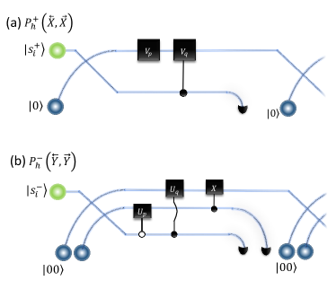
Figure 3: Quantum circuits for generating (a) and (b) . Here (black circle and line) is the standard control gate . Meanwhile (white circle, black line) is defined as . (a) To simulate we initialize a qubit in state and an ancilla in state . Executing the local unitary , followed by the 2-qubit gate , where , creates a suitable entangled state – such that a computation basis measurement of the top qubit yields , and simultaneously collapses the bottom qubit into the causal state for the next time step. (b) To simulate we prepare state as input. Execution of where , followed by where satisfies , and finally where is the Pauli X operator generates a suitable entangled state – such that measuring the first two qubits yields (provided we identify measurement outcome , and ), and collapses the remaining qubit into the quantum causal state for the next time step. In either circuit, retaining only the state of (green circle) at each time-step is sufficient for generating statistically correct predictions or retrodictions.
II Results
We study this question via two complementary approaches. The first is a case study of the heralding coin - the aforementioned process that exhibits causal asymmetry. We pioneer methods to establish its provably optimal quantum causal and retrocausal models, and thus produce a precise picture of how quantum mechanics mitigates all present causal asymmetry. The second studies quantum modelling of arbitrary processes with causal asymmetry. Here, and cannot be directly evaluated, but can nevertheless be bounded. In doing so, we show that when forced to model such process in the less natural direction, the quantum advantage always exceeds the memory overhead .
The Heralding Coin – Let denote the heralding coin process. Here we first state the optimal quantum models of and . We then outline how their optimality is established, leaving details of the formal proof to Appendix B.
The optimal causal model has two internal states;
(3)
with associated encoding function if-and-only-if . Given a qubit in state , Fig. 3 establishes the sequential proccedure that replicates expected future behaviour, i.e., samples .
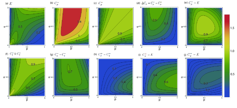
Figure 4: Complexity of the heralding coin plotted against and . The figure illustrates across all values of the parameter space (). (d) depicts the classical causal asymmetry , and (f) effectively demonstrates and thus .
Meanwhile the optimal quantum retrocausal model has encoding function if-and-only-if , where
(4)
The associated procedure for sequential generation of as governed by is outlined in Fig. 3.
To establish optimality, we first invoke the causal state correspondence: for any stochastic process with causal states that occur with probability , there exists an optimal model , where the elements of are in 1-1 correspondence with (see Lemma 1 of Appendix A). Since the heralding coin process has two forward causal states, we can restrict
our computation of to quantum models where . Moreover we can show that the data processing inequality implies (see Lemma 2 of Appendix A). The monotonicity between and the entropy of the resulting model, together with observation that , then implies optimality of (see Theorem 1 of Appendix B). This establishes for .
Proving the optimality of is more involved. First note the causal state correspondence allows us to consider only candidate models where has three elements. The data processing inequality can then be used to establish the fidelity constraints (see Lemma 2 of Appendix A). Let with eigenvalues , and with eigenvalues . In Lemma 4 of Appendix B, we prove that for all choices of satisfying the fidelity constraint majorizes . Thus has minimal entropy among all valid retrocausal quantum models.
and exhibit different encoding functions (one maps onto two code words, the other onto three), and invoke seemingly unrelated quantum circuits for generating future statistics (see Fig. 3). Nevertheless direct computation yields
(5)
where and is the binary entropy. Thus for all values of and . This establishes our first result:
Result 1.
There exists stochastic processes that are causally asymmetric (), but exhibit no such asymmetry when modelled quantum mechanically ().
This vanishing of causal asymmetry at the quantum level is not simply the result of saturating the bound given by . Fig. 4 shows that for almost all values of and . While both quantum causal and retrocausal models reduce memory resources beyond classical limits (i.e., and , see Fig 4 f and g), they each still store some unnecessary information (, see Fig. 4 i).
Our results persist when considering minimal dimensions, rather than minimal entropy required for causal modelling. requires only two causal states, and thus can be modeled using a -level system (). , however, has three causal states. Modelling it thus requires a -level system (). In contrast, the three quantum causal states of can be embedded within a single qubit, and thus the dynamics of the heralding coin can be modelled using a single qubit in either temporal direction. Therefore this vanishing of causal asymmetry also applies in single shot settings.
General Processes – We now study quantum mitigation of causal asymmetry for general stochastic processes by bounding and from above. Let represent the minimum amount of information we need to classically model when allowed to optimize over temporal direction. Meanwhile let be the minimal memory a quantum system needs when forced to model the process in the least favourable temporal direction. In Appendix C, we establish the following:
Result 2.
For any stochastic process ,
(6)
Equality occurs only if , such that is causally symmetric.
Consider any causally asymmetric process , such that modelling it in the less favourable temporal direction incurs memory overhead . Result 2 implies that this overhead can be entirely mitigated by quantum models. There exists a quantum model that is not only provably simpler than its optimal classical counterpart, but is also simpler than any classical model of the time-reversed process . In Lemma 7 (see Appendix C), we show that such models can be systematically constructed, and align with the simplest currently known quantum models – -machines Mahoney et al. (2016); Binder et al. (2017). As a corollary, causal asymmetry guarantees both and , i.e., non-zero quantum advantage exists when modelling in either causal direction.
A variant of these results also applies to topological state complexity. Suppose the number of causal states for and its time-reversal differ, such that . Let and respectively be the logarithm of the minimal dimensions needed to model and quantum mechanically. Appendix C also establishes that
Result 3.
For any stochastic process ,
(7)
Given there exists stochastic processes where predictive and retrodictive topological complexity differ (e.g. the heralding coin). This immediately implies the following corollary:
Result 4.
The quantum topological complexity can be strictly less than the classical topological complexity .
This solves an open question in quantum modelling - whether quantum mechanics allows for models that simulate stochastic processes using not only reduced memory, but also reduced dimensions.
These results have particular impact when is exceedingly large. Recall that in the case of the - flower process, while scales as . Our theorem then implies that . Thus we immediately identify a class of processes whose optimal classical models require a memory that scales as , and yet can be modelled quantum mechanically using a single qutrit.
III Future Directions
There are a number of potential relations between causal asymmetry and innovations on the arrow of time, and retrodictive quantum theory. In this section, we survey some of these connections, and highlight promising future research directions.
Retrodictive Quantum Mechanics – Consider the evolution of an open quantum system that is monitored continuously in time. Standard quantum trajectory theory describes how the system’s internal state evolves, encapsulating how our expectations of future measurement outcomes update based on past observations. Retrodictive quantum mechanics introduces the effect matrix – a time-reversed analogue of the density matrix Dressel (2015); Gammelmark et al. (2013); Wiseman (2002). propagates backwards through time, representing how our expectations of the past change as we scan future measurement outcomes in time-reversed order. The original motivation was that and combined yield a more accurate estimate of the measurement statistics at time than alone, allowing improved smoothing procedures Tan et al. (2015); Rybarczyk et al. (2015); Weber et al. (2014); Campagne-Ibarcq et al. (2014).
While this framework and causal asymmetry differ in motivation and details (e.g. monitoring is done in continuous time, whereas we have so far only considered discrete time), there are also notable coinciding concepts. The standard propagation equation for parallels a causal model for observed measurement statistics, while its time-reversed counterpart governing parallels a corresponding retrocausal model. It would certainly be interesting to see if such systems exhibit either classical or quantum causal asymmetry. For example, does the resource cost of tracking differ from that of under some appropriate measure 444Note that since and vary over a continuum, the memory costs of tracking either is likely to be unbounded. Thus one may need to modify present approaches. Existing approaches include the use of differential entropies Marzen and Crutchfield (2017) and studying scaling as we track the process to greater precision Garner et al. (2017b)?
Answering these questions will likely involve significant extensions of current results. Our framework presently assumes the process evolves autonomously, and that time is divided into discrete steps. These restrictions will need to be lifted, by combining present results with recent generalizations of classical and quantum computational mechanics to continuum time Marzen and Crutchfield (2017); Elliott and Gu (2018) and input-dependent regimes Barnett and Crutchfield (2015); Thompson et al. (2017); Cabello et al. (2016). More generally, such developments will enable a formal study of causal asymmetry in the quantum trajectories formulation of open quantum systems.
Arrow of Time in Quantum Measurement – Related to such open systems are recent proposals for inferring an arrow of time from continuous measurement Dressel et al. (2017). These proposals consider continuously monitoring a quantum system initialized in state , resulting in a measurement record with some probability . Concurrently, the state of the system evolves through a quantum trajectory , into some final configuration . The goal is to identify an alternative sequence of measurements, such that for at least one possible outcome record occurring with non-zero probability , the trajectory rewinds. That is, a system initially in state will evolve into , passing through all intermediary states in time-reversed order. An arrow of time emerges as and generally differ, such that one of the two directions occurs with greater probability. An argument via Bayes’ theorem then assigns different probabilistic likelihoods towards whether occurred in forward or reverse time.
This framework provides a complementary perspective to our results. It aims to reverse the trajectory of the system’s internal state , placing no constraints on the relation between the measurement statistics governing and . In contrast, causal asymmetry deals with reversing the observed measurement statistics (as described by some stochastic process ), while placing no restrictions on the internal dynamics of the causal and retrocausal models (the two models may even field different Hilbert space dimensions, such as in the heralding coin example).
We also observe some striking parallels. Both works start out with some sequential data, but no knowledge about whether the sequence occurred in forward or reverse time. Both ask the following question: Is there some sort of asymmetry singling out one temporal direction over the other? In the emerging arrow of time from quantum measurement, we are given a trajectory , and asymmetry arises from the difficulty (in terms of success probability) of realizing this trajectory in forward versus reverse time. Meanwhile, in causal asymmetry, we are given the observed measurement statistics, and an arrow of time arises from the difference in resource costs needed to realize these statistics causally in forward versus reverse time. It would then be interesting to see if a similar argument via Bayes’ theorem can be adapted to causal asymmetry. Supposing more complex machines are less likely to exist in nature (e.g. due to dimensional or entropic constraints), could we then argue whether a given stochastic process is more likely to occur in one causal direction versus the other?
IV Discussion
Causal asymmetry captures the memory overhead incurred when modelling a stochastic process in one temporal order versus the other. This induces a privileged temporal direction when one seeks the simplest causal explanation. Here we demonstrate a process where this overhead is non-zero when using classical models, and yet vanishes when quantum models are allowed. For arbitrary processes exhibiting causal asymmetry, we prove that quantum models forced to operate in a given temporal order always require less memory than classical counterparts, even when the latter are permitted to operate in either temporal direction. The former result represents a concrete case where causal asymmetry vanishes in the quantum regime. The latter implies that the more causally asymmetric a process, the greater the resource advantage of modelling it quantum mechanically.
Our results also hold when memory is quantified by max entropy. They thus establish that quantum mechanics can reduce the dimensionality needed to simulate a process beyond classical limits. Indeed our results isolate families of processes whose statistical complexity grows without bound, but can nevertheless be modelled exactly by a quantum system of bounded dimension. These features make such processes ideal for demonstrating the practical benefits of quantum models – allowing us to verify arbitrarily large quantum advantage in single-shot regimes Konig et al. (2009); Dahlsten (2013), and avoiding the need to measure von Neumann entropy as in current state of the art experiments Palsson et al. (2017).
One compelling open question is the potential thermodynamic consequences of causal asymmetry. In computational mechanics, has thermodynamical relevance in the contexts of prediction and pattern manipulation Wiesner et al. (2012); Garner et al. (2017a); Boyd et al. (2017); Still et al. (2012); Cabello et al. (2016). For instance, the minimum heat one must dissipate to generate future predictions based on only past observations is given by , where is Boltzmann’s constant, is the environmental temperature, and the excess entropy is symmetric with respect to time-reversal. Therefore, non-zero causal asymmetry implies that flipping the temporal order in which we ascribie predictions incurs an energetic overhead of . In processes where scales without bound, this cost may become prohibitive. Could our observation that imply such energetic penalties become strongly mitigated when quantum simulators are taken into account?
A second direction is to isolate what properties of quantum processing enable it to mitigate causal asymmetry. In Appendix C, we establish that all deterministic processes are causally symmetric, such that (see Lemma
6 of Appendix C). Randomness is therefore essential for causal asymmetry. Observe also that the provably optimal quantum causal and retrocausal models for the heralding coin both operated unitarily – such that their dynamics are entirely deterministic (modulo measurement of outputs). Indeed, such unitary quantum models can always be constructed Binder et al. (2017), and we conjecture that this unitarity implies causal symmetry. However, it remains an open question as to whether the optimal quantum model is always unitary.
Insights here will ultimately help answer the big outstanding question of whether the quantum statistical complexity ever displays asymmetry under time-reversal. Identifying any process for which such asymmetry persists implies that Occam’s preference for minimal cause can privilege a temporal direction in a fully quantum world. Proof that no such process exists would be equally exciting, indicating that causal asymmetry is a consequence of enforcing all causal explanations to be classical in a fundamentally quantum world.
Acknowledgements – The authors appreciated the feedback and input received from: Yang Chengran, Suen Whei Yeap, Liu Qing, Alec Boyd, Varun Narasimhachar, Felix Binder, Thomas Elliott, Howard Wiseman, Geoff Pryde, Nora Tischler, Farzad Ghafari and Chiara Marletto. This work was supported by, the National Research Foundation of Singapore and in particular NRF Awards NRF-NRFF2016-02, NRF-CRP14-2014-02 and RF2017-NRF- ANR004 VanQuTe, the John Templeton Foundation grants 52095 and 54914, Foundational Questions Institute grant FQXi-RFP-1609 and Physics of the Observer grant No. FQXi-RFP-1614, the Oxford Martin
School, the Singapore Ministration of Education Tier 1 RG190/17 and the U. S. Army Research Laboratory and the U. S. Army Research Office under contracts No. W911NF-13-1-0390, No. W911NF-13-1-0340, and No. W911NF-18-1-0028. Much of the collaborative was also made possible by the ‘Interdisciplinary Frontiers of Quantum and Complexity Science’ workshop held in January 2017 in Singapore, funded by the John Templeton Foundation, the Centre for Quantum Technologies and the Lee foundation of Singapore.
Appendix A Technical Definitions
We first introduce further technical notation and background that will be used for subsequent proofs.
Definition 1(Quantum Causal Model).
Consider an ordered tuple where is a set of quantum states; is an encoding function that maps each
onto a state of a physical system ; and is a quantum process. is a quantum model for if-and-only-if for any , whenever is prepared in subsequent application of : (i) generates an output with probability and (ii) transitions into a new state where Suen et al. (2017).
Condition (i) guarantees that if a quantum model is initialized in state then the model’s future output will be statistically indistinguishable from the output of the process itself. (ii) ensures the internal memory of the quantum model updates to record the event , allowing the model to stay synchronized with the sequence of outputs it has generated thus far. Thus a series of repeated applications of acting on , generates output with probability , and simultaneously transitions into the state . In the limit , the model produces a sequence of outputs with probability .
The entropy of a quantum model is given by
(8)
where is the von Neumann entropy, for , and .
Definition 2.
is an optimal quantum model for a process , if given any other model , we have .
Consider a stationary stochastic process , such that for any , . Let have causal states each occurring with stationary probability . Define the conditional distribution as the future morph of causal state . We will make use of the following two results derived in Suen et al. (2017).
Lemma 1(Causal state correspondence).
Let be a stochastic process with causal states . There exists an optimal model where and if-and-only-if .
This implies that we can limit our search for optimal models , to those whose internal states are in one-to-one correspondence with the classical causal states. In addition, it can be shown that must satisfy the following constraint:
Lemma 2(Maximum fidelity constraint).
Let be a stochastic process with causal states , and be a valid quantum model satisfying iff . Then , where is the fidelity between the future morphs of and .
These definitions assume that all elements of are pure. This is because computational mechanics considers only causal models – models whose internal states do not store more information about the future than what is available from the past. Specifically, let be a random variable governing the state of a model at . is then known as the oracular information, and represents the amount of extra information contains about the future that is not contained in the past
. For causal models, Crutchfield et al. (2010). In Appendix E, we show that this allows us to assume all elements of are pure without loss of generality.
Appendix B Proofs of Optimality
Here, we formally prove that the quantum models for the heralding coin given in Eq. (II) and Eq. (II) are optimal.
B.1 Optimality of the Causal Model.
Let denote the heralding coin process, with corresponding -machine depicted in Fig. 2(a).
Theorem 1.
Consider , where if-and-only-if , with
(9)
, and described by the quantum circuit in Fig. 3(a). is an optimal quantum model for .
Proof.
We prove this by contradiction. Assume there exists some such . Lemma 1 implies that we can assume for some and and encoding function if-and-only-if , without loss of generality. , the von-Neumann entropy of the ensemble , is a monotonically decreasing function of Jozsa and Schlienz (2000). Thus implies that . Meanwhile, Lemma 2 implies
(10)
This is a contradiction. Thus no such exists.
∎
B.2 Optimality of the Retrocausal Model.
Let denote the time reversal of the heralding coin process, with corresponding -machine in Fig. 2(b).
Theorem 2.
Define , where if-and-only-if , with
(11)
, and the measurement process given in Fig. 3(b). is an optimal quantum model for .
Below we break the proof of this theorem down into a series of small steps. Each step is phrased as a lemma.
Lemma 3.
Let be a quantum model for satisfying iff . Then, up to a unitary rotation,
(12)
for some , , , such that and .
Proof.
Set . Explicit evaluation yields , , . By the maximum fidelity constraint, . Thus . Therefore and up to a unitary rotation. We can then write in the form above without loss of generality as the coefficient of can be made real and positive by choosing a suitable definition of basis element . Meanwhile constraints on and imply and . ∎
Our models described in Eq. (II) can be obtained by setting and in Eq. (3) (i.e. this corresponds to choosing , and ). The subsequent lemma then establishes that this is the optimal choice.
Lemma 4.
For any quantum model of satisfying if-and-only-if .
(13)
That is, , as described by Eq. (II), is the lowest entropy (optimal) model which satisfies the causal state correspondence.
Proof.
By definition for , where and the states are given in Eq. (II). We label the eigenvalues of this state from largest to smallest by . Meanwhile by the above lemma where
and is described by Eq. (3). We label the eigenvalues of from largest to smallest by . To establish that it is sufficient to show , where denotes majorization Nielsen and Vidal (2001). This is established by proving that (1) and (2) .
We begin by establishing . By the minimax principle Courant and Hilbert (1953), the largest eigenvalue for is
(14)
Suppose that this maximum is attained for some such that
(15)
where , and . We can assume the coefficient of is real and positive because Eq. (14) remains unchanged when . Substituting Eq. (15) into Eq. (14) yields
(16)
We defined to be the vector that maximizes Eq. (16); and thus we have implicitly optimized over and in Eq. (16). This optimization will automatically set (since any two complex numbers satisfy ). Using this and trigonometry identities to simplify Eq. (16), yields
(17)
We now show that there always exists some such that . The maximum fidelity constraint implies . Thus there exists some such that , (in particular we choose the solution of this equation where ). Consider
where
(18)
for . Furthermore let be defined as
(19)
for . Then we have
(20)
where we have used the fact that and . Specifically these two conditions imply and . Thus we have .
To show , we define to be the state satisfying . In general we can parameterize
for , , and . Using the same argument as in Eq. (17), we can show and thus
Define . By mirroring the analysis in Eq. (20) we find
(22)
Together the above results imply , establishing step (1) .
For step (2) We must show . However by construction only spans a 2-dimensional Hilbert space and thus we have . It follows that . Together, these results imply and therefore .
∎
By Lemma 1, has an optimal quantum model which satisfies the causal state correspondence. Meanwhile by Lemma 4, any satisfying the causal state correspondence must have . It follows that is an optimal quantum model for .
Here we prove Result 2. To do this, we require some preliminary lemmas. The first connects the capacity for quantum models to improve upon their optimal classical counterparts with causal asymmetry.
Lemma 5.
If the classical and quantum statistical complexity of a process coincide, such that , then is causally symmetric and .
Proof.
We first make use of the prior results showing that whenever classical models waste information, more efficient quantum models exist Gu et al. (2012). Specifically if-and-only-if . Thus, implies that . It is therefore sufficient to show that implies .
We prove this by contradiction. Assume but . Now implies , where is the random variable governing the causal state at Shalizi and Crutchfield (2001). Thus given we can find a unique such that is only non-zero when . It follows that the sets form a partitioning on the space of all futures (i.e. for ).
Furthermore any two satisfy , by definition of . Thus Bayes’ theorem implies that the partition the future into equivalence classes if-and-only-if 555 To derive this simply write .. Hence constitute the retrocausal states. Bayes’ theorem also yields only when . This implies , where governs the retrocausal state at time . Hence , which is a contradiction.
∎
It follows as a direct corollary of this result that causal asymmetry vanishes for deterministic processes (i.e. processes where ).
Lemma 6.
Any deterministic process has .
Proof.
Any deterministic process has Mahoney et al. (2011); Shalizi and Crutchfield (2001). Since it follows that and thus according to the above lemma .
∎
Our next lemma makes use of q-machines Mahoney et al. (2016), the simplest currently known quantum models. Consider a process whose classical -machine has a collection of causal states and transition probabilities . Let denote the cryptic order of , defined as the smallest such that Riechers et al. (2016); Mahoney et al. (2016, 2011). The q-machine of has internal states defined by a recursive relation
(23)
(24)
and . The associated encoding function satisfies whenever Riechers et al. (2016); Mahoney et al. (2016).
Let be the -machine complexity – the amount of information a -machine stores about the past, where . Meanwhile let the max entropy be the q-machine state complexity – the minimum dimensionality of any quantum system capable of storing these internal states. Note that since q-machines are valid quantum models, and . Likewise and . We now establish that the -machine for and its time-reversal have coinciding Von Neumann entropies and coinciding max entropies.
Lemma 7.
Let be a stationary stochastic process and its time reversal with q-machine complexity and , and q-machine state complexity and respectively. Then , and
Proof.
We first introduce some compact notation. Let similarly , as well as and .
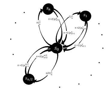
Figure 5: The - flower process, illustrated for the case , and even. Physically this process can be generated by a set of -sided dice where each dice is biased, so that it lands on side with probability (and in general the bias on each dice is different, such that for ). We randomly select a dice , recording the choice . Afterwards we role the dice, transcribing the outcome as .
Now let denote the internal states of the q-machine for , such that , and . From existing work Mahoney et al. (2016); Riechers et al. (2016), we know that . Thus let , and such that . Then
(25)
Furthermore the forward q-machine complexity is given by . A similar argument shows that is given by , where
(26)
Consider now the pure state
(27)
which represents that quantum superposition, or q-sample Aharonov and Ta-Shma (2003), over all possible output strings of the stochastic process , with associated density operator
(28)
We can verify that and . Thus and therefore . The -machine complexity of the forward and backward processes thus coincide.
Note that the rank of and must also coincide. Thus, an analogous argument establishes that , indicating the two models also have the same dimensionality. Therefore .
∎
We now prove Result 2. Consider any stochastic process . First assume is causally asymmetric, such that . Note first that this implies (by Lemma 5). Meanwhile Lemma 7 implies that . Thus it is sufficient to show that and , whenever .
Note that for a general process, , if-and-only-if the q-machine has two internal states with non-zero overlap Nielsen and Chuang (2000). It is also previously established that that whenever , we can find some Gu et al. (2012), as defined by Eq. (23). It follows from the iterative construction that , and thus . Therefore implies and implies . Hence, for any causally asymmetric
(29)
Conversely, suppose . Without loss of generality, we can assume . This implies either (i) or (ii) . In the case of (i), direct application of Lemma 5 implies . In the case of (ii) we have , which implies . That is, -machines are not more efficient than -machines in modelling . This is true if-and-only-if Gu et al. (2012); Riechers et al. (2016). Thus Lemma 5 again implies . This completes the proof.
Appendix D - flower process
The family of - flower processes demonstrate how causal asymmetry can be potential unbounded (see Fig. 5). The process has statistical complexity . In contrast, the time reversed process will have at most causal states and thus . Meanwhile the predictive and retrodictive topological state complexities satisfy and . and can be adjusted independently. Setting , and allowing , yields diverging but finite . Thus also diverges to infinity. A similar divergence is witness for topological state complexity.
Applying Result 2, we see that and are both bounded above by . The same is also true for and . Thus, quantum models of this process can fit within a single qutrit, whether modelling in forward or reverse time. In the specific case of the former, and diverge to infinity. Thus, we obtain a family of processes whose quantum models field unbounded memory advantage - in both the entropic and single-shot sense.
Appendix E Excluding Mixed State Models
In this section we consider more general causal models which have the freedom to encode pasts
(30)
into mixed quantum states. We show that this does not allow for models which are more optimal than those which only encode pasts into pure quantum states.
Theorem 3.
Consider a stochastic process , with a causal model . If the internal states of are mixed, such that , then we can always find a causal model such that , and .
Proof.
Let have causal states . Suppose is an optimal causal model for , with mixed internal states.
It is trivial to generalize the causal state correspondence to mixed state models. Thus we can assume that has an encoding function where
(31)
if-and-only-if . So that the internal states are in 1-1 correspondence with the classical causal states.
Our proof makes use of the requirement that causal models store no oracular information, i.e. where is the random variable governing the memory. Regrouping the pasts into causal state equivalence classes yields , where is the probability the past belongs to . Thus for every .
We have assumed some elements of are mixed. In particular, suppose we have a specific with that occurs with probability . Let
be a particular past such that , and be a set of pure states that form an unravelling of . I.Fe. there must exist some such that . Now let be a quantum process that maps to a classical random variable governed by probability distribution . By definition of a quantum model, this process can always be constructed by concatenations of acting on a physical system .
Let represent the state of and be the random variable that governs the resulting output of acting on . Zero oracular information implies that and must be uncorrelated when conditioned on observing past
. Therefore for all .
Now consider the entropy of . By concavity of entropy
Without loss of generality we can assume this minimum is obtained for . Let be
a set of internal states where is replaced with , and define encoding function such that except when , whereby . Define a new quantum model . Clearly .
If any of the states in are still mixed, then by repeating the above procedure we can replace them with pure states, thereby constructing a model with pure internal states such that
∎
References
Linden et al. (2009)Noah Linden, Sandu Popescu,
Anthony J Short, and Andreas Winter, “Quantum mechanical evolution
towards thermal equilibrium,” Physical Review E 79, 061103 (2009).
Popescu et al. (2006)Sandu Popescu, Anthony J Short, and Andreas Winter, “Entanglement and
the foundations of statistical mechanics,” Nature Physics 2, 754 (2006).
Page and Wootters (1983)Don N Page and William K Wootters, “Evolution
without evolution: Dynamics described by stationary observables,” Physical Review
D 27, 2885 (1983).
Price (1997)Huw Price, Time’s arrow &
Archimedes’ point: new directions for the physics of time (Oxford University Press, USA, 1997).
Crutchfield et al. (2009)James P Crutchfield, Christopher J Ellison, and John R Mahoney, “Time’s barbed arrow: Irreversibility, crypticity, and stored
information,” Physical review letters 103, 094101 (2009).
Crutchfield (2012)James P Crutchfield, “Between
order and chaos,” Nature Physics 8, 17–24 (2012).
Note (1)Formally, this implies that the conditional mutual
information is
zero, where is the random variable governing the state of . In
literature, is
named oracular information, as it captures the amount of information a state
of the memory stores about the future that is not contained in the
past Ellison et al. (2011); Crutchfield et al. (2010). Note
that this notion of causal model differs from the recent developments in
quantum causal models Allen et al. (2017); Costa and Shrapnel (2016) and
foundation work on causal inference Pearl (2009).
Crutchfield and Young (1989)James P Crutchfield and Karl Young, “Inferring
statistical complexity,” Physical Review Letters 63, 105 (1989).
Shalizi and Crutchfield (2001)Cosma Rohilla Shalizi and James P Crutchfield, “Computational mechanics: Pattern and prediction, structure and
simplicity,” Journal of statistical physics 104, 817–879 (2001).
Park et al. (2007)Joongwoo Brian Park, Jeong Won Lee, Jae-Suk Yang, Hang-Hyun Jo, and Hie-Tae Moon, “Complexity analysis of the
stock market,” Physica A: Statistical Mechanics and its Applications 379, 179–187 (2007).
Tino and Koteles (1999)Peter Tino and Miroslav Koteles, “Extracting
finite-state representations from recurrent neural networks trained on
chaotic symbolic sequences,” IEEE Transactions on Neural Networks 10, 284–302 (1999).
Cabello et al. (2018)Adán Cabello, Mile Gu, Otfried Gühne, and Zhen-Peng Xu, “Optimal
classical simulation of state-independent quantum contextuality,” Physical Review
Letters 120, 130401
(2018).
Garner et al. (2017a)Andrew JP Garner, Jayne Thompson, Vlatko Vedral, and Mile Gu, “Thermodynamics of complexity and pattern manipulation,” Physical Review E 95, 042140 (2017a).
Wiesner et al. (2012)Karoline Wiesner, Mile Gu, Elisabeth Rieper, and Vlatko Vedral, “Information-theoretic lower bound on energy cost of stochastic
computation,” in Proceedings
of the Royal Society of London A: Mathematical, Physical and Engineering
Sciences, Vol. 468 (The
Royal Society, 2012) pp. 4058–4066.
Cabello et al. (2016)Adán Cabello, Mile Gu, Otfried Gühne, Jan-Åke Larsson, and Karoline Wiesner, “Thermodynamical
cost of some interpretations of quantum theory,” Physical Review A 94, 052127 (2016).
Boyd et al. (2017)Alexander B Boyd, Dibyendu Mandal, Paul M Riechers, and James P Crutchfield, “Transient dissipation and structural costs of physical information
transduction,” Physical Review Letters 118, 220602 (2017).
Note (2)Note that in computational mechanics literature, causal
asymmetry is often referred to as causal irreversibility Crutchfield et al. (2009). Here, we choose the term causal asymmetry to avoid
confusion with standard notions of irreversibility used in the physics
community.
Konig et al. (2009)Robert Konig, Renato Renner,
and Christian Schaffner, “The
operational meaning of min-and max-entropy,” IEEE Transactions on Information theory 55, 4337–4347 (2009).
Suen et al. (2017)Whei Yeap Suen, Jayne Thompson, Andrew J. P. Garner, Vlatko Vedral,
and Mile Gu, “The classical-quantum
divergence of complexity in the ising spin chain,” Quantum 1, 25 (2017).
Note (3)Note that while these definitions implicitly assume we can
only encode onto pure states . We show in Appendix E that even
when we allow the encoding function to map directly onto mixed quantum
states, it does not help – there is always a pure state quantum causal model
with entropy (see Theorem 3).
Gu et al. (2012)Mile Gu, Karoline Wiesner,
Elisabeth Rieper, and Vlatko Vedral, “Quantum mechanics can reduce
the complexity of classical models,” Nature communications 3, 762 (2012).
Riechers et al. (2016)Paul M Riechers, John R Mahoney, Cina Aghamohammadi, and James P Crutchfield, “Minimized state complexity of quantum-encoded cryptic processes,” Physical Review
A 93, 052317 (2016).
Palsson et al. (2017)Matthew S Palsson, Mile Gu, Joseph Ho, Howard M Wiseman,
and Geoff J Pryde, “Experimentally modeling
stochastic processes with less memory by the use of a quantum processor,” Science Advances 3, e1601302 (2017).
Tan et al. (2014)Ryan Tan, Daniel R Terno,
Jayne Thompson, Vlatko Vedral, and Mile Gu, “Towards quantifying complexity with quantum
mechanics,” Eur.
Phys. J. Plus 129, 191
(2014).
Monras and Winter (2016)Alex Monras and Andreas Winter, “Quantum learning
of classical stochastic processes: The completely positive realization
problem,” Journal of Mathematical Physics 57, 015219 (2016).
Garner et al. (2017b)Andrew JP Garner, Qing Liu, Jayne Thompson,
Vlatko Vedral, and Mile Gu, “Provably unbounded memory advantage in
stochastic simulation using quantum mechanics,” New Journal of Physics 19, 103009 (2017b).
Mahoney et al. (2016)John R Mahoney, Cina Aghamohammadi, and James P Crutchfield, “Occam’s quantum strop: Synchronizing and compressing classical cryptic
processes via a quantum channel,” Scientific reports 6
(2016).
Binder et al. (2017)Felix C Binder, Jayne Thompson, and Mile Gu, “A practical, unitary
simulator for non-markovian complex processes,” arXiv preprint arXiv:1709.02375 (2017).
Dressel (2015)Justin Dressel, “Weak values as
interference phenomena,” Physical Review A 91, 032116 (2015).
Gammelmark et al. (2013)Søren Gammelmark, Brian Julsgaard, and Klaus Mølmer, “Past quantum states of a monitored system,” Physical review letters 111, 160401 (2013).
Wiseman (2002)HM Wiseman, “Weak values,
quantum trajectories, and the cavity-qed experiment on wave-particle
correlation,” Physical Review A 65, 032111 (2002).
Tan et al. (2015)Dian Tan, SJ Weber, Irfan Siddiqi, K Mølmer, and KW Murch, “Prediction and retrodiction for a continuously monitored
superconducting qubit,” Physical review letters 114, 090403 (2015).
Rybarczyk et al. (2015)T Rybarczyk, B Peaudecerf, M Penasa,
S Gerlich, Brian Julsgaard, Klaus Mølmer, S Gleyzes, M Brune, JM Raimond, S Haroche,
et al., “Forward-backward analysis of the photon-number evolution in a cavity,” Physical Review
A 91, 062116 (2015).
Weber et al. (2014)SJ Weber, Areeya Chantasri, Justin Dressel, Andrew N Jordan, KW Murch, and Irfan Siddiqi, “Mapping the optimal route
between two quantum states,” Nature 511, 570 (2014).
Campagne-Ibarcq et al. (2014)Philippe Campagne-Ibarcq, Landry Bretheau, Emmanuel Flurin, Alexia Auffèves, François Mallet, and Benjamin Huard, “Observing interferences between past and future
quantum states in resonance fluorescence,” Physical review letters 112, 180402 (2014).
Note (4)Note that since and vary over a continuum,
the memory costs of tracking either is likely to be unbounded. Thus one may
need to modify present approaches. Existing approaches include the use of
differential entropies Marzen and Crutchfield (2017) and studying scaling
as we track the process to greater precision Garner et al. (2017b).
Marzen and Crutchfield (2017)Sarah Marzen and James P Crutchfield, “Informational and causal architecture of continuous-time renewal
processes,” Journal of Statistical Physics 168, 109–127 (2017).
Elliott and Gu (2018)Thomas J Elliott and Mile Gu, “Superior memory efficiency of quantum devices for the simulation of
continuous-time stochastic processes,” npj Quantum Information 4, 18 (2018).
Barnett and Crutchfield (2015)Nix Barnett and James P Crutchfield, “Computational mechanics of input–output processes: Structured
transformations and the epsilon ϵ-transducer,” Journal of
Statistical Physics 161, 404–451 (2015).
Thompson et al. (2017)Jayne Thompson, Andrew JP Garner, Vlatko Vedral,
and Mile Gu, “Using quantum theory to
simplify input–output processes,” npj Quantum Information 3, 6 (2017).
Dressel et al. (2017)Justin Dressel, Areeya Chantasri, Andrew N Jordan, and Alexander N Korotkov, “Arrow of time for continuous quantum measurement,” Physical review letters 119, 220507 (2017).
Dahlsten (2013)Oscar CO Dahlsten, “Non-equilibrium statistical mechanics inspired by modern information
theory,” Entropy 15, 5346–5361
(2013).
Still et al. (2012)Susanne Still, David A Sivak,
Anthony J Bell, and Gavin E Crooks, “Thermodynamics of
prediction,” Physical review letters 109, 120604 (2012).
Crutchfield et al. (2010)James P Crutchfield, Christopher J Ellison, Ryan G James, and John R Mahoney, “Synchronization and control in intrinsic and designed computation: An
information-theoretic analysis of competing models of stochastic
computation,” Chaos: An Interdisciplinary Journal of Nonlinear Science 20, 037105 (2010).
Jozsa and Schlienz (2000)Richard Jozsa and Jürgen Schlienz, “Distinguishability of states and von neumann entropy,” Physical Review A 62, 012301 (2000).
Nielsen and Vidal (2001)Michael A Nielsen and Guifré Vidal, “Majorization and the interconversion of bipartite states.” Quantum Information &
Computation 1, 76–93
(2001).
Courant and Hilbert (1953)R Courant and D Hilbert, Methods of mathematical
physics, vol. I (Interscience, 1953).
Note (5)To derive this simply write .
Mahoney et al. (2011)John R Mahoney, Christopher J Ellison, Ryan G James,
and James P Crutchfield, “How hidden
are hidden processes? a primer on crypticity and entropy convergence,” Chaos: An
Interdisciplinary Journal of Nonlinear Science 21, 037112 (2011).
Aharonov and Ta-Shma (2003)Dorit Aharonov and Amnon Ta-Shma, “Adiabatic
quantum state generation and statistical zero knowledge,” in Proceedings of the thirty-fifth annual ACM
symposium on Theory of computing (ACM, 2003) pp. 20–29.
Nielsen and Chuang (2000)Michael A Nielsen and Isaac L Chuang, “Quantum
computation and quantum information,” (2000).
Ellison et al. (2011)Christopher J Ellison, John R Mahoney, Ryan G James, James P Crutchfield, and Jörg Reichardt, “Information symmetries in irreversible processes,” Chaos: An
Interdisciplinary Journal of Nonlinear Science 21, 037107 (2011).
Allen et al. (2017)John-Mark A Allen, Jonathan Barrett, Dominic C Horsman, Ciarán M Lee, and Robert W Spekkens, “Quantum common causes and quantum causal models,” Physical Review X 7, 031021 (2017).
Costa and Shrapnel (2016)Fabio Costa and Sally Shrapnel, “Quantum causal
modelling,” New
Journal of Physics 18, 063032 (2016).
Pearl (2009)Judea Pearl, “Causal inference
in statistics: An overview,” Statistics surveys 3, 96–146 (2009).