Photodissociation dynamics in the first absorption band of pyrrole: I. Molecular Hamiltonian and the Herzberg-Teller absorption spectrum for the ${}^{1}\!A_{2}(\pi\sigma^{*})\leftarrow\widetilde{X}^{1}\!A_{1}(\pi\pi)$ transition

Abstract

This paper opens a series in which the photochemistry of the two lowest $\pi\sigma^{*}$ states of pyrrole and their interaction with each other and with the ground electronic state $\widetilde{X}$ are studied using ab initio quantum mechanics. New 24-dimensional potential energy surfaces for the photodissociation of the N—H bond and the formation of the pyrrolyl radical are calculated using the CASPT2 method for the electronic states $\widetilde{X}(\pi\pi)$, $1^{1}\!A_{2}(\pi\sigma^{*})$ and $1^{1}\!B_{1}(\pi\sigma^{*})$ and locally diabatized. In the first paper, the ab initio calculations are described and the photodissociation in the state $1^{1}\!A_{2}(\pi\sigma^{*})$ is analyzed. The excitation $1^{1}\!A_{2}\leftarrow\widetilde{X}$ is mediated by the coordinate dependent transition dipole moment functions constructed using the Herzberg-Teller expansion. Nuclear dynamics, including 6, 11, and 15 active degrees of freedom, is studied using the multi-configurational time-dependent Hartree method. The focus is on the frequency resolved absorption spectrum, as well as on the dissociation time scales and the resonance lifetimes. Calculations are compared with available experimental data. An approximate convolution method is developed and validated, with which absorption spectra can be calculated and assigned in terms of vibrational quantum numbers. The method represents the total absorption spectrum as a convolution of the diffuse spectrum of the detaching H-atom and the Franck-Condon spectrum of the heteroaromatic ring. Convolution calculation requires a minimal quantum chemical input and is a promising tool for studying the $\pi\sigma^{*}$ photodissociation in model biochromophores.

I Introduction

This and the subsequent two papers (termed ‘Paper II’PG17B and ‘Paper III’PDG17 ) describe the results of an ab initio quantum dynamical study of the absorption spectra, non-adiabatic dynamics, and the photofragment distributions of pyrrole, C₄H₄NH, photoexcited with ultraviolet (UV) light with the wavelengths $\lambda$ between 250 nm and 220 nm. Pyrrole, which acts as a chromophore unit in porphyrins and in the amino acid tryptophan, is a characteristic example of a molecule exhibiting the so-called $\pi\sigma^{*}$ photochemistry.SDDJ02 ; MKAD16 Photodissociation in the considered wavelength range occurs in the first two excited singlet electronic states of ${}^{1}\pi\sigma^{*}$ character which are dissociative along the N—H bond and form conical intersections with the ground electronic state. This paper gives our motivation behind the study, describes the construction of the full-dimensional molecular Hamiltonian for the three electronic states involved, and discusses the absorption spectra due to the lowest ${}^{1}\pi\sigma^{*}$ state. Paper II focuses on the photofragment distributions in this state. Paper III analyzes the non-adiabatic photodissociation dynamics in the two ${}^{1}\pi\sigma^{*}$ states coupled to the ground electronic state.

The atomistic mechanisms of non-radiative decay of the initial electronic excitation in aromatic molecules, serving as models of broad classes of UV biochromophores, are actively studied using experiment and theory (see Refs. WKRRT03, ; LRHR04, ; DCNA06, ; HWRBPS11, ; MCOFCL12, ; CBYEU11, ; RWPUS12, ; ADDKNO08, ; ACDDN06, ; NDCDA06, ; NDCA06, ; GYBU15, ; OKA11, ; ZTBPT15, ; AKMNOS10, ; RS14, ; MKAD16, ; SDDJ02, ; LDVSM05, ; VLMSD05, ; BLSM09, ; YXZT14, ; ZY16, ; XMZYXG16, ; BKPMKTS10, ; KPNWF17, and references therein). In the gas phase, the internal energy of the UV excited pyrrole is large enough to allow dissociation into several chemically distinct channels. One group of channels is populated on a nanosecond time scaleMICHLBONACIC90 and is reached via electronic relaxation to the ground electronic state $\widetilde{X}$ along the ring-deformation and ring-opening pathways.BNL94 ; WKRRT03 ; RS14 ; BLSM09 ; ZTBPT15 ; MKAD16 In contrast, dissociation into hydrogen atom and pyrrolyl radical via ${}^{1}\pi\sigma^{*}$ electronic states occurs on a sub-picosecond time scale.LRHR04 ; ACDDN06 ; NDCDA06 ; AKMNOS10 ; OKA11 ; RS14 The ${}^{1}\pi\sigma^{*}$ states often lack oscillator strength (especially if compared to the optically ‘bright’ ${}^{1}\pi\pi^{*}$ states), but their potential energy surfaces are repulsive or only weakly bound, and this topographic feature allows them to control ultrafast electronic relaxation pathways.SDDJ02 ; AKMNOS10 ; RS14 The ${}^{1}\pi\sigma^{*}$ state mediated H-atom detachment in heteroaromatic molecules is an actively expanding research field, and a range of powerful spectroscopic techniques — both high resolution frequency resolvedAKMNOS10 and ultrafast time resolvedRS14 ; S14 ; ZTBPT15 ; KPNWF17 — are applied to monitor the reaction fragments. The experimental studies are complemented by ab initio theoretical methodsSDDJ02 ; LDVSM05 ; CBYEU11 ; MSMS15 ; XMZYXG16 ; KPNWF17 providing a convincing interpretation in terms of the electronic structure and quantum dynamics calculations.

The first absorption band of pyrrole [see Fig. 1(a)], extending from 5.0 eV to 6.5 eV, was extensively studied in the past. While its complete electronic assignment remains a subject of hot discussions, most researches currently agree that the weak structureless absorption at the longest wavelengths, highlighted in the left part of panel (a), is due to the two lowest excited ${}^{1}\pi\sigma^{*}$ states. Their one-dimensional (1D) potential energy curves along the dissociation coordinate are illustrated in Fig. 2(a,b). The lowest excited singlet state $1^{1}\!A_{2}(\pi\sigma^{*})$ (with the vertical excitation energy $T_{v}$ of about 5.0 eV) arises mainly from the promotion of an electron from the $1a_{2}(\pi)$ to the $10a_{1}(3s/\sigma^{*})$ Rydberg molecular orbital; the transition from the ground electronic state $\widetilde{X}^{1}\!A_{1}(\pi\pi)$ (hereafter referred to as $\widetilde{X}$) is electric dipole forbidden and is accomplished via the vibronic intensity borrowing. The second $\pi\sigma^{*}$ state, located $\sim 1.0$ eV above $1^{1}\!A_{2}$, is the state $1^{1}\!B_{1}(\pi\sigma^{*})$. It originates mainly from the $2b_{1}(\pi)\rightarrow 10a_{1}(3s/\sigma^{*})$ orbital excitation and, although its excitation from $\widetilde{X}$ is electric dipole allowed, the oscillator strength of this transition is tiny. It is therefore not surprising that the absorption cross sections of both $\pi\sigma^{*}$ states are small. Panel (b) of Fig. 1 illustrates the absorption band calculated in this work for the state $1^{1}\!A_{2}(\pi\sigma^{*})$ coupled to $\widetilde{X}$. The calculated peak intensity at 4.6 eV does not exceed $2.5\times 10^{-20}$ cm², and in experiment the band is overlayed by the shoulder of a much stronger absorption of the higher lying ${}^{1}\pi\pi^{*}$ states.CNQA04 ; NW14 The absorption of the state $1^{1}\!B_{1}(\pi\sigma^{*})$, discussed in paper III and not shown in Fig. 1(b), is somewhat stronger (it reaches $10^{-19}$ cm² around 5.8 eV) but is still very weak.

The $\pi\sigma^{*}$ states in Fig. 2(a,b) are repulsive with respect to the extension of the N—H bond; the state $1^{1}\!A_{2}(\pi\sigma^{*})$ correlates with the photofragments in their electronic ground states, ${\rm H}(^{1}\!S)+{\rm pyrrolyl}(\widetilde{X}^{2}\!A_{2})$, while the state $1^{1}\!B_{1}(\pi\sigma^{*})$ correlates with the first excited state $1^{2}\!B_{1}$ of pyrrolyl. Both $\pi\sigma^{*}$ states feature shallow local minima in the Franck-Condon (FC) zone separated from the asymptotic region by low barriers, indicating that a tunneling contribution to the dissociation can be expected.VLMSD05 ; WNSSAWS15 ; XDFG16 In the exit channel, away from the FC zone, both $\pi\sigma^{*}$ states form conical intersections (CIs) with the ground electronic state; the CIs are marked with circles in Fig. 2(a,b). The intersections are symmetry allowed: The exact degeneracies are found in $C_{2v}$ symmetric configurations and involve states belonging to different irreps of the $C_{2v}$ point group. The totally symmetric dissociation coordinate $R$ acts as a tuning mode, while the coupling modes have $a_{2}$ symmetry for the $\widetilde{X}/A_{2}$ CI and $b_{1}$ symmetry for the $\widetilde{X}/B_{1}$ CI. These CIs, predicted by Sobolewski, Domcke, and co-workers on the basis of general symmetry arguments,SDDJ02 are the most salient features of the $\pi\sigma^{*}$ states in pyrrole and, as argued in Ref. MKAD16, , in many other model biochromophores. Located in the exit dissociation channel, these CIs strongly affect the molecular photoreactivity and, in particular, influence the vibrational state distributions and the kinetic energy release of the photofragments.PG14 ; PG15 In a recent quantum mechanical study, we discovered their fingerprints in the absorption spectra as strongly asymmetric Fano resonances.GP17A

With the aim to understand the dynamics at these exit channel CIs, the weakest portion of the first absorption band, located below 5.7 eV, has been extensively studied in the frequency- and time domain by many experimental and theoretical groups. The H-atom Rydberg tagging photofragment translational spectroscopy studies of Ashfold and co-workersCNQA04 ; CDNA06 ; AKMNOS10 interrogated the formation of the fragment hydrogen atom for a series of photolysis wavelengths $\lambda$ between 254 nm and 190 nm. The key observable in these experiments is the total kinetic energy release (TKER) in the photodissociation reaction. In the two-fragment channel ${\rm H}+{\rm pyrrolyl}$, the TKER spectra are equivalent to the rovibrational distributions of the pyrrolyl radical. The observed kinetic energy distributions are bimodal,CNQA04 with the fast (average kinetic energy $E_{\rm kin}\geq 4000$ cm^-1) and the slow ($E_{\rm kin}\sim 1000$ cm^-1) components well resolved for most wavelengths. The angular distributions of the fast fragments are typically anisotropic (non-zero recoil anisotropy parameter), while the slow components correspond to isotropically distributed fragments. These observations led experimentalists AKMNOS10 ; CNQA04 to associate the fast products with the direct dissociation in the excited $\pi\sigma^{*}$ electronic states and to assume that the slow products emerge as a result of statistical decomposition in the ground electronic state reached via internal conversion. In line with this assignment, two well separated dissociation time constants were established in the pump-probe measurements performed close to the absorption origin near $\lambda=250$ nm:LRHR04 The time $\tau_{d}=110$ fs was attributed to the direct reaction, and the time $\tau_{s}=1.1$ ps was associated with the statistical dissociation. Recent ultrafast time-resolved experiments at the same wavelength of 250 nm confirmed the fast time scale (the reported value was $\tau_{d}=126$ fs) and also argued that this is a tunneling lifetime.RWYCYUS13 The same group found a much shorter dissociation time of $\tau_{d}=46$ fs for $\lambda=238$ nm. Even shorter lifetimes of $19$ fs and $12$ fs were found for $\lambda=236$ nm and 242 nm, respectively, in the time resolved photoelectron measurements of Wu et al.WNSSAWS15 The measured dependence of $\tau_{d}$ on the photolysis wavelength is non-monotonous, and this conclusion is reinforced by the recent time resolved study of Ref. KPNWF17, .

Theoretical studies of the electronic structure, spectroscopy, and photochemistry of pyrrole are numerous. Accurate multireference ab initio calculations of vertical excitation energies clarified the ordering of the low lying valence and Rydberg excited states.VLMSD05 ; BVAEML06 ; FVSELK11 ; RMMSM02 ; CW03 ; SBL09 The branching ratios of several arrangement channels, including ring deformation and ring opening reactions, were simulated using classical trajectory surface hopping algorithm.BVAEML06 ; SBL09 Multi-dimensional multi-state quantum dynamics investigations of the ultrafast electronic population dynamics in the excited states of pyrrole were performed by Köppel, Lischka, and co-workers.FVSELK11 Recently, Neville and WorthNW14 studied the first absorption band using ab initio Hamiltonian constructed as an extension of the quadratic vibronic coupling model and including the first seven electronic states. These studies yielded important insight into the radiationless decay dynamics of pyrrole, provided new vibronic assignments of the intense features between 5.5 eV and 6.5 eV, and gave theoretical estimates of the dissociation lifetimes in the $1^{1}\!A_{2}(\pi\sigma^{*})$ stateNW14 ; WNSSAWS15 between 35 fs and 133 fs, in general agreement with experiment.

Despite these efforts, several key questions related to the $\pi\sigma^{*}$ states of pyrrole require further investigation. In the frequency domain, the absorption spectrum of the two lowest $\pi\sigma^{*}$ states remains virtually unexplored; the only published spectra of these states were synthesized by Roos et al. from harmonic frequencies and vertical excitation energies 15 years ago.RMMSM02 The wavelength resolved TKER distributions measured by Ashfold and co-workersCNQA04 have neither been calculated nor assigned theoretically. In the time domain, the tunneling contribution to the sub-picosecond dissociation in the $1^{1}\!A_{2}(\pi\sigma^{*})$ state has not been quantified. A univocal assignment of the measured reaction time scales remains outstanding, and the fluctuations in the dependence of the measured dissociation times $\tau_{d}$ on the photon energy are not explained.

We recently launched a systematic investigation of the photodissociation of pyrrole photoexcited into the states $1^{1}\!A_{2}(\pi\sigma^{*})$ and $1^{1}\!B_{1}(\pi\sigma^{*})$. The primary goal is to provide a comprehensive picture of the photodissociation dynamics: To analyze the weak diffuse absorption bands, to assign them in terms of the vibrational quantum numbers, to evaluate the photodissociation time scales, and to compare the resulting TKER distributions with the frequency resolved measurements of Ashfold and co-workers. In this opening paper of the series, new high level ab initio calculations are described which are performed on a coordinate grid uniformly covering the inner FC zone and the asymptotically separated H-atom and pyrrolyl. These calculations serve as a basis for construction of a new 24-dimensional (24D) molecular Hamiltonian of pyrrole in a local quasi-diabatic representation. The Hamiltonian is next used in the quantum dynamical calculations of photodissociation. The Hamiltonian is inspired by the reaction path formalismMHA80 ; CM84 extended to three electronic states; the constructed diagonal quasi-diabatic potentials are chosen harmonic only in the degrees of freedom of the pyrrolyl fragment. Further, the coordinate dependences of the transition dipole moment (TDM) vectors are explicitly included within the framework of the Herzberg-Teller expansion.BUNKERJENSEN06 In this way, direct excitation of these optically dark states is enabled. Paper I focuses on the absorption spectrum of the state $1^{1}\!A_{2}(\pi\sigma^{*})$, both isolated and coupled to the ground electronic state $\widetilde{X}$. The TKER distributions in this state are analyzed in paper II.PG17B It is paper IIIPDG17 which extensively deals with the three-state effects and with the photodissociation dynamics in the second excited state $1^{1}\!B_{1}(\pi\sigma^{*})$.

The second, methodological, goal of this study is the development of simplified computational schemes within which the diffuse absorption in the repulsive $\pi\sigma^{*}$ states and the subsequent sub-picosecond formation of the photofragments can be quantitatively analyzed. The aim is to construct computational tools for dissociating systems which require a minimal ab initio input and a numerical effort not exceeding that of a standard FC factor calculation of bound-bound transitions in polyatomic molecules. In paper I, a convolution approximation for the absorption spectra is introduced, which casts the total spectrum as a convolution of the absorption spectra due to the departing H-atom and due to the pyrrolyl ring. In paper II, a related overlap integral-based mapping method for the TKER distributions is proposed.

The remainder of the paper is organized as follows: The details of the electronic structure calculations and the design of the 24D molecular Hamiltonian comprising the states $\widetilde{X}$, $1^{1}\!A_{2}(\pi\sigma^{*})$, and $1^{1}\!B_{1}(\pi\sigma^{*})$ are presented in Sect. II. The quantum mechanical methods and the convolution approximation are summarized in Sect. III and in two Appendices. The resulting absorption spectra are discussed in Sect. IV. While the emphasis here is on the dissociation in the isolated state $1^{1}\!A_{2}(\pi\sigma^{*})$, dissociation in the coupled pair $\widetilde{X}/1^{1}\!A_{2}(\pi\sigma^{*})$ is also considered and the effects inherent to the two-state dynamics are highlighted. Conclusions are given in Sect. V.

II Construction of the molecular Hamiltonian

II.1 The form of the 24 dimensional Hamiltonian

The molecular Hamiltonian,

$$\hat{\underline{{\bf H}}}=\hat{T}\,\underline{{\bf 1}}+\left(\begin{array}[]{ccc}V^{X}&V^{XA_{2}}&V^{XB_{1}}\\ V^{XA_{2}}&V^{A_{2}}&V^{A_{2}B_{1}}\\ V^{XB_{1}}&V^{A_{2}B_{1}}&V^{B_{1}}\end{array}\right)\,,$$ (1)

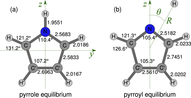
Figure 3: The SA-CASSCF(8,7)/CASPT2/aug-cc-pVTZ+ equilibrium geometries of the ground states of pyrrole and pyrrolyl are shown in panel (a) and (b). Bond distances are in $a_{0}$. Also shown are the Cartesian coordinate system used in the calculation of the TDMs (panel (a); the axis $x$ is perpendicular to the molecular plane) and the definition of the disappearing modes $R$ and $\theta$ [panel (b)]. The azimuthal angle $\phi$ is defined relative to the $x$ axis in the $xy$ plane. $(\theta,\phi)=(0^{\circ},0^{\circ})$ corresponds to the H-atom on the axis $z$; $(\theta\neq 0,\phi=0^{\circ})$ describes the H-atom in the plane $xz$; $(\theta\neq 0,\phi=90^{\circ})$ describes the H-atom in the plane $yz$.

is set in the basis of three locally diabatic electronic states $\widetilde{X}$ (its $C_{2v}$ symmetry label is $A_{1}$), $A_{2}$, and $B_{1}$ illustrated in Fig. 2(a,b). Bold faced underlined symbols are used for $3\times 3$ matrices ($\underline{{\bf 1}}$ is the unit matrix). Pyrrole is described using (i) three Jacobi coordinates $\mathbf{R}\equiv(R,\theta,\phi)$ of the dissociating H-atom with respect to the center of mass of the pyrrolyl fragment [the so-called ‘disappearing modes’; see Fig. 3(b)] and (ii) 21 dimensionless normal modes $\mathbf{Q}$ of pyrrolyl, calculated at the equilibrium geometry of the fragment (the so-called ‘non-disappearing modes’). The normal modes $\mathbf{Q}$ are partitioned into four blocks according to the irreps $\Gamma$ of the $C_{2v}$ point group, $\mathbf{Q}=\{\mathbf{Q}_{a_{1}},\mathbf{Q}_{a_{2}},\mathbf{Q}_{b_{1}},\mathbf{Q}_{b_{2}}\}$.

The kinetic energy operator in Eq. (1) is set for the zero total angular momentum of pyrrole in the frame of the body-fixed principal axes (atomic units are used hereafter):

$$\hat{T} = \hat{T}_{R}+\hat{T}_{Q}$$ (2)

$$= -\frac{1}{2m_{R}}\frac{\partial^{2}}{\partial R^{2}}+\frac{\hat{{\bm{j}}}^{2}}{2m_{R}R^{2}}+\frac{1}{2}\left(\frac{\hat{j}_{x}^{2}}{I_{x}}+\frac{\hat{j}_{y}^{2}}{I_{y}}+\frac{\hat{j}_{z}^{2}}{I_{z}}\right)-\frac{1}{2}\sum_{\begin{subarray}{c}\Gamma=a_{1},a_{2},\\ \ \ b_{1},b_{2}\end{subarray}}{\sum_{i}}^{\Gamma}\omega_{\Gamma}(i)\frac{\partial^{2}}{\partial{Q_{\Gamma}(i)}^{2}}\,.$$

The kinetic energy $\hat{T}_{R}$ of the disappearing modes comprises the first three terms including the kinetic energy of the relative motion of H-atom and pyrrolyl ($m_{R}$ is the corresponding reduced mass), the orbital motion of the H-atom, and the rotational motion of the rigid pyrrolyl ring, respectively; $\hat{\bm{j}}=(\hat{j}_{x},\hat{j}_{y},\hat{j}_{z})$ is the pyrrolyl angular momentum operator and the inertia constants $I_{x}$, $I_{y}$ and $I_{z}$ are evaluated at pyrrolyl equilibrium. The term $\hat{T}_{Q}$ refers to pyrrolyl vibrations; the sum $\sum_{i}^{\Gamma}$ is over the vibrational modes $i$ belonging to an irrep $\Gamma$. The $C_{2v}$ symmetric pyrrolyl ring lies in the $yz$-plane, with $z$ being the $C_{2}$ axis (see Fig. 3).

The quasi-diabatic potential energy matrix in Eq. (1) is constructed as a sum of two matrices:

$$\underline{{\bf V}}(\mathbf{R},\mathbf{Q})=\underline{{\bf U}}_{R}(\mathbf{R})+\underline{{\bf W}}_{Q}(\mathbf{Q}|R)\,;$$ (3)

Elements of the matrix $\underline{{\bf U}}_{R}(\mathbf{R})$ depend on the three disappearing modes $(R,\theta,\phi)$ only; they are spline interpolations of the quasi-diabatized energies on a dense ab initio three-dimensional (3D) grid in $\mathbf{R}$. Elements of the matrix $\underline{{\bf W}}_{Q}(\mathbf{Q}|R)$ depend on the 21 non-disappearing modes $\mathbf{Q}$. These 21D functions are constructed in the spirit of the vibronic coupling model of Ref. KDC84, . The pyrrolyl ring is treated using quadratic Hamiltonians, and the parameters of the vibronic coupling model depend on the interfragment distance $R$ (but not on the angles $\theta$ and $\phi$). The structure of the Hamiltonian of Eq. (1) is similar to that adopted in the work of Neville and Worth.NW14 The difference is in the choice of the disappearing modes $\mathbf{R}$ (here: three Jacobi coordinates), in the choice of the coordinate grids (here: the coordinate grid uniformly covers the complete dissociation path), and in the construction of the matrices $\underline{{\bf U}}_{R}(\mathbf{R})$ and $\underline{{\bf W}}_{Q}(\mathbf{Q}|R)$ (here: spline interpolations on a regular grid).

The diagonal elements of the potential matrix have the form ($\alpha=X,A_{2},B_{1}$):

$$V^{\alpha}(R,\theta,\phi,\mathbf{Q}) = U_{R}^{\alpha}(\mathbf{R})+W_{Q}^{\alpha}(\mathbf{Q}|R)$$ (4)

$$= U^{\alpha}_{\rm 1D}(R)+U^{\alpha}_{\rm ang}(R,\theta,\phi)$$

$$+{\sum_{i}}^{a_{1}}\kappa^{\alpha}_{i}(R)Q_{a_{1}}(i)+\frac{1}{2}\sum_{\Gamma}{\sum_{i,j}}^{\Gamma}\gamma^{\alpha}_{\Gamma,ij}(R)Q_{\Gamma}(i)Q_{\Gamma}(j)\,.$$

$U^{\alpha}_{\rm 1D}(R)$ are the one-dimensional potential energy functions along $R$, with $(\theta,\phi)=(0^{\circ},0^{\circ})$, and the ring modes set to the pyrrolyl equilibrium $\mathbf{Q}=\mathbf{0}$; $U_{\rm ang}^{\alpha}(R,\theta,\phi)$ are the distance-dependent angular potentials vanishing for $(\theta,\phi)=(0^{\circ},0^{\circ})$ [the relation between the pair $(\theta,\phi)$ and the molecular configurations is exemplified in the caption to Fig. 3(b)]. Functions $\kappa_{i}^{\alpha}(R)$ are the $R$-dependent gradients vanishing for all modes but $a_{1}$. Functions $\gamma_{ij}^{\alpha}(R)$ are the $R$-dependent Hessians with respect to normal modes. Both $\kappa_{i}^{\alpha}(R)$ and $\gamma_{ij}^{\alpha}(R)$ are evaluated at $\mathbf{Q}=\mathbf{0}$. Hessian matrices ${\bm{\gamma}}^{\alpha}$ are four-block diagonal: $\bm{\gamma}^{\alpha}=\bm{\gamma}^{\alpha}_{a_{1}}\oplus\bm{\gamma}^{\alpha}_{a_{2}}\oplus\bm{\gamma}^{\alpha}_{b_{1}}\oplus\bm{\gamma}^{\alpha}_{b_{2}}$.

The off-diagonal diabatic couplings $V^{\alpha\beta}$ are given by

$$V^{\alpha\beta}(R,\theta,\phi,\mathbf{Q}) = U_{R}^{\alpha\beta}(\mathbf{R})+W_{Q}^{\alpha\beta}(\mathbf{Q}|R)$$ (5)

$$= U^{\alpha\beta}_{\mathrm{ang}}(R,\theta,\phi)+{\sum_{i}}^{\Gamma_{\alpha}\times\Gamma_{\beta}}\lambda^{\alpha\beta}_{i}(R)Q_{\Gamma_{\alpha}\times\Gamma_{\beta}}(i)\ ,$$

Functions $U^{\alpha\beta}_{\mathrm{ang}}(R,\theta,\phi)$ are constructed on the 3D coordinate grid by first applying the regularized diabatization procedure of Köppel et al.KGM01 to the raw adiabatic ab initio energies and next interpolating between grid points using cubic splines. While $U^{\alpha\beta}_{\mathrm{ang}}(R,\theta,\phi)$ do not have an analytical representation, near the CIs with $\widetilde{X}$ the construction algorithm ensures that they follow the lowest allowed orders in the symmetry-adapted spherical harmonics, namely $U^{XA_{2}}_{\mathrm{ang}}\sim\sin^{2}\theta\sin(2\phi)$ and $U^{XB_{1}}_{\mathrm{ang}}\sim\sin\theta\cos\phi$. The $\mathbf{Q}$-dependent couplings $W_{Q}^{\alpha\beta}(\mathbf{Q}|R)$ are linear in the ring modes: The $X/A_{2}$ and $X/B_{1}$ coupling terms are promoted by the vibrational modes of $a_{2}$ and $b_{1}$ symmetry, respectively. The matrix element $W^{A_{2}B_{1}}$ between the states $A_{2}/B_{1}$ is not included in the quantum mechanical calculations.

The quasi-diabatic representation used in the Hamiltonian of Eq. (1) is local, i.e. a given off-diagonal matrix element $V^{\alpha\beta}$ is non-zero only in a (broad) vicinity of the CI between states $\alpha$ and $\beta$, where a non-vanishing transition probability between quasi-diabatic states is expected. For the second term in Eq. (5), this is achieved by using the following functional form for the coupling strength $\lambda_{i}^{\alpha\beta}$:

$$\lambda_{i}^{\alpha\beta}(R)=\lambda_{\mathrm{CI},i}^{\alpha\beta}\exp\left(-\left|\frac{R-R_{\mathrm{CI}}^{\alpha\beta}}{\Delta}\right|^{n}\right)\ ,$$ (6)

where $R_{\mathrm{CI}}^{\alpha\beta}$ is the position of the CI between $\alpha/\beta=X/A_{2}$ or $X/B_{1}$. The parameters $\lambda_{\mathrm{CI},i}^{\alpha\beta}$, $\Delta$ and $n$ are tuned ‘by eye’ in order to obtain smooth diabatic Hessians for the coupled states. Similar attenuation functions are applied to the mixing angles of the regularized adiabatic-to-diabatic transformation in $(R,\theta,\phi)$. Examples of the local diabatic coupling functions are given in Fig. 2(b).

II.2 Ab initio parameterization of the molecular Hamiltonian

II.2.1 Quantum chemical calculations

The matrix elements of the molecular Hamiltonian, Eqs. (1), (4), and (5), are constructed from the ab initio energies obtained using the electronic structure calculations performed with the aug-cc-pVTZ (AVTZ) basis set of Dunning.D89 The basis set is further augmented with the diffuse $s$ and $p$ functions added to the N and H atoms of the dissociating bond (one set of $s$ and $p$ functions for N and two sets for H). The exponents of these functions are derived in an even tempered manner from the most diffuse $s$ and $p$ functions of the AVTZ basis by dividing the exponents successively by a factor of 3.0.VLMSD05 This extension is necessary to correctly describe the Rydberg character of the states $1^{1}\!A_{2}(\pi\sigma^{*})$ and $1^{1}\!B_{1}(\pi\sigma^{*})$, and the resulting basis set is referred to as AVTZ+.

Most calculations are performed at the CASPT2 level of theory. The reference wavefunctions are obtained from the state-averaged CASSCF calculations including the states $\widetilde{X}^{1}A_{1}$, $1^{1}\!A_{2}(\pi\sigma^{*})$ and $1^{1}\!B_{1}(\pi\sigma^{*})$. The active space comprises five $\pi$ valence molecular orbitals, three of $b_{1}$ and two of $a_{2}$ symmetry, the $9a_{1}(\sigma)$ and the $10a_{1}(3s/\sigma^{*})$ orbitals.NOTE-PYR01A-01 This setting for the active space, consisting of eight electrons in seven orbitals, will be denoted as $(8_{e},7_{o})$. The choice of this relatively small active space guarantees that the ab initio calculations are running smoothly for small as well as asymptotic interfragment distances $R$. Electronic structure calculations are performed using the highest possible symmetry. The matrix elements of the potential matrix $\underline{{\bf U}}_{R}(\mathbf{R})$ are calculated as functions of the disappearing modes using the symmetry group $C_{1}$. The blocks of the $\mathbf{Q}$-dependent Hessian matrices with symmetries $a_{1},\ a_{2},\ b_{1}\ \mbox{and}\ b_{2}$ are calculated separately using $C_{2v}$, $C_{2}$, $C_{s}$ and $C_{s}^{\prime}$ symmetries, respectively. Coordinate dependent TDM functions, necessary to properly describe the optical excitation of the $\pi\sigma^{*}$ states from the ground electronic state, are calculated at the CASSCF level. In addition to the main batches, several sets of benchmark calculations were performed with the AVTZ+ basis set using the multi-reference configuration interaction (with Davidson correction applied,LD74 MRCI+Q) and the equation of motion coupled cluster (EOM-CCSD) methods. In all calculations, MOLPRO suite of programs was used.MOLPRO-FULL

The first step in the construction of matrix elements is the calculation of the minimum energy path (MEP) for hydrogen detachment from the N—H group in the first excited state $1^{1}\!A_{2}(\pi\sigma^{*})$. The MEP is calculated along the Jacobi coordinate $R$; the grid $\{R_{i}\}$ consists of 28 points lying between $R_{\rm min}=3.5\,a_{0}$ and $R_{\rm max}=8.3\,a_{0}$. Along this path, the molecule is constrained to $C_{2v}$ geometries with $(\theta,\phi)=(0^{\circ},0^{\circ})$. In the subsequent steps, the full dimensional quasi-diabatic representation is built using this MEP as a reference. This is conceptually similar to the reaction surface HamiltonianMHA80 ; CM84 with the difference that a single set of normal modes is used along the MEP. Finally, in order to simulate the excitation process, the geometry of pyrrole in the ground electronic state is also optimized and used as a reference for the calculation of the Herzberg-Teller TDM. The optimized structures of pyrrole and pyrrolyl are compared in Fig. 3. The main structural changes in going from the parent to the radical are the increase of the $\mathrm{C-C^{\prime}}$ bond (by $0.16\ a_{0}$) and the decrease of the $\mathrm{C^{\prime}-C^{\prime}}$ bond (by $0.14\ a_{0}$).

II.2.2 3D diabatic potentials for the disappearing modes

The CASPT2 energies of the lowest three electronic states are calculated on a three-dimensional grid $(R_{i},\theta_{j},\phi_{k})$, with the nodes $R_{i}$ being grid points on the MEP. The grid points $\theta_{j}$ in the polar angle cover the range $[0^{\circ},90^{\circ}]$ with a step of 5^∘; for a set of $R_{i}$ values, calculations over the range $[0^{\circ},180^{\circ}]$ are performed, and the remaining missing energies for $\theta>90^{\circ}$ are extrapolated. The grid in the azimuthal angle $\phi$ ranges from $0^{\circ}$ to $90^{\circ}$ with a step of 15^∘; energies for larger $\phi$ are reconstructed using $C_{2v}$ symmetry of the pyrrolyl ring. The 1D cuts along $\theta$ and $\phi$ are exemplified in Fig. 2(c,d). In all three states, the geometries with $(\theta,\phi)=(0^{\circ},0^{\circ})$ correspond to a minimum. In the excited states, this minimum is local and the hydrogen atom lying in the plane of the ring has to overcome a potential barrier in order to reach the out-of-plane geometries with $\theta>20^{\circ}$. Thus the calculation predicts that pyrrole in the excited $\pi\sigma^{*}$ states remains near-planar in the initial stages of dissociation.

Quasi-diabatic representation for the calculated states is constructed in two steps. In the first step, the states $\widetilde{X}$ and $1^{1}\!A_{2}(\pi\sigma^{*})$ are diabatized. The angular modes do not couple them at either $\phi=0^{\circ}$ or $90^{\circ}$, and the impact of $\theta$ and $\phi$ on the non-adiabatic dynamics in the $X/A_{2}$ pair is exceedingly weak. For this reason, the states $\widetilde{X}$ and $1^{1}\!A_{2}(\pi\sigma^{*})$ can be diabatized by a relabeling the adiabatic energies. The tiny coupling matrix element between these states for $\phi\neq 0,90^{\circ}$, is modeled as

$$U^{XA_{2}}_{R}(R,\theta,\phi)=\lambda^{XA_{2}}_{\rm ang}(R)\sin^{2}\theta\sin(2\phi)\,,$$ (7)

with the $R$-dependent function $\lambda^{XA_{2}}_{\rm ang}(R)=c\left[1-{\rm atan}\left((R-R_{0})/\Delta R\right)\right]$. The parameters $c$, $R_{0}$, and $\Delta R$ are chosen ‘by eye’ in order to give smooth diabatic curves for a full range of $\phi$.

In the second step, the states $\widetilde{X}$ and $1^{1}\!B_{1}(\pi\sigma^{*})$ are transformed to the quasi-diabatic representation. The orthogonal transformation between the diagonal matrix of the adiabatic energies of $\widetilde{X}$ and $1^{1}\!B_{1}(\pi\sigma^{*})$ and the non-diagonal diabatic potential matrix is effected by the $2\times 2$ adiabatic-to-diabatic transformation matrix $\underline{{\bf S}}(\mathbf{R})$,

$$\underline{{\bf S}}(\mathbf{R})=\left(\begin{array}[]{lr}\cos\Theta&-\sin\Theta\\ \sin\Theta&\cos\Theta\end{array}\right)$$ (8)

where $\Theta$ is the coordinate dependent mixing angle constructed with the regularized diabatic state method of Köppel et al.KGM01 To this end, two potential energy differences between adiabatic states are used. One, denoted $\Delta_{1}$, is evaluated in the $C_{2v}$ symmetric subspace $(R,\theta,\phi)=(R,0,0)$ along the Jacobi coordinate $R$. Another, denoted $\Delta_{2}$, is evaluated for the $C_{1}$ subspace $(R_{\mathrm{CI}}^{XB_{1}},\theta,\phi)$ with the distance $R$ fixed at the CI degeneracy point. The mixing angle is defined as

$$\Theta=\frac{1}{2}\arctan\frac{\Delta_{2}}{\Delta_{1}}\,.$$ (9)

By construction, the diabatic potential matrix elements in the vicinity of the degeneracy point are linear in the displacements from $(R_{\mathrm{CI}}^{XB_{1}},0,0)$, i.e. $U^{X},\,U^{B_{1}}\sim(R-R_{\mathrm{CI}}^{XB_{1}})$ and $U^{XB_{1}}\sim\sin\theta\cos\phi$. Away from the degeneracy point, the mixing angle $\Theta$ is attenuated with the function of the form of Eq. (6), so that the adiabatic-to-diabatic transformation is localized to the intersection region. Finally, all diabatic matrix elements set on the grid are interpolated using cubic splines. It is ensured that they become independent of the disappearing angles $\theta$ and $\phi$ as $R$ reaches the asymptotic region $R>7.0\,a_{0}$.

1D cuts through the potential energy surfaces of the three diabatic states are shown in Fig. 2. The minimum of the $\widetilde{X}$ state [panel (a)] is located at $R\approx 4.1\ a_{0}$. In the excited states, local minima are found at $4.23\ a_{0}$ for $1^{1}\!A_{2}(\pi\sigma^{*})$ and at $4.14\ a_{0}$ for $1^{1}\!B_{1}(\pi\sigma^{*})$. These minima are separated by $\leq 0.10$ eV high barriers from the repulsive portions of the potential curves. The energy parameters of the ab initio PESs are summarized in Tables 1 and 2 which are discussed in the next section.

Two-dimensional (2D) contour plots of the splined diabatic potentials $\widetilde{X}$ and $1^{1}\!A_{2}(\pi\sigma^{*})$ in the $(R,\theta)$ plane are shown in Fig. 4; the contour plots for the state $1^{1}\!B_{1}(\pi\sigma^{*})$ are discussed in Paper III. In the ground electronic state, the coordinates $R$ and $\theta$ are strongly mixed in the FC zone, around $R=4.15\,a_{0}$ and $(\theta,\phi)=(0^{\circ},0^{\circ})$: Contour lines around the potential minimum have a characteristic ‘banana’ shape indicating that the equilibrium pyrrolyl—H distance shrinks as the H-atom moves out of the plane of the pyrrolyl ring. In the potential $U^{X}_{R}(R,\theta,\phi)$, the quantum mechanical (anharmonic) out-of-plane bending frequency of the H-atom (along $\theta$, $\phi=0^{\circ}$) is of the order of $406$ cm^-1 which is about three times lower than the anharmonic in-plane bending frequency of $\sim 1281$ cm^-1 (along $\theta$, $\phi=90^{\circ}$). In the state $1^{1}\!A_{2}(\pi\sigma^{*})$, $R$ and $\theta$ are also mixed, and the height of the dissociation barrier around $R\approx 4.7\,a_{0}$ depends on $\theta$. The barrier of $0.09$ eV (cf. Table 1) along the straight dissociation path with $\theta=0$ is always the lowest, which is yet another indication that almost no torque along $\theta$ is exerted on the H-atom in the initial stage of the photodissociation in the state $1^{1}\!A_{2}(\pi\sigma^{*})$.

II.2.3 21D diabatic potentials for the non-disappearing modes

The parameters of the $\mathbf{Q}$-dependent part of the diabatic Hamiltonian matrix are calculated as first and second derivatives with respect to deviations from the MEP in the state $1^{1}\!A_{2}(\pi\sigma^{*})$. The $C_{2v}$ symmetry is preserved along the MEP, and the raw ab initio energies and their first derivatives are diabatized by a trivial relabeling of the calculated points. Most ab initio second derivatives (i.e., elements of the Hessian matrices) are also in this ‘trivially diabatic’ form. Exceptions are Hessian blocks involving symmetry breaking coupling modes and diverging near the CIs; diabatization is required in order to remove the resulting singularities and to fix the diabatic coupling strengths $\lambda_{i}^{\alpha\beta}$. The Hamiltonian matrix is constructed in the following sequence of ab initio calculations and transformations:

1. Geometry optimization and the normal mode analysis for the ground electronic state $\widetilde{X}^{2}\!A_{2}$ of pyrrolyl. In this step, the dimensionless normal coordinates $\mathbf{Q}$ of pyrrolyl are defined. They are related to the Cartesian coordinates $\mathbf{X}$ of the atoms via the rectangular transformation matrix $\underline{{\bf L}}$ with elements $L_{ir}$:

   $$Q_{i}=\sum_{r=1}^{27}\sqrt{\frac{\omega_{i}M_{r}}{\hbar}}F_{ir}X_{r}=\sum_{r=1}^{27}L_{ir}X_{r}\ ,i=1,21\,,$$ (10)

   where $M_{r}$ is the mass of the atom associated with the coordinate $X_{r}$, $\omega_{i}$ is the frequency of the normal mode $Q_{i}$, and $\{F_{ir}\}$ is the matrix of eigenvectors of the mass-weighted Cartesian Hessian from which the rows corresponding to the rigid pyrrolyl translations and rotations are removed. The values of normal modes along the MEP are denoted $\mathbf{Q}=\mathbf{Q}_{\mathrm{min}}(R)$.

2. Calculation of the Cartesian gradient vectors $\{\bar{g}_{i}^{\alpha}\}$ and Hessian matrices $\{\bar{\gamma}_{\Gamma,ij}^{\alpha}\}$. They are calculated for $\alpha=X$, $A_{2}$, and $B_{1}$ along the MEP. The gradients and Hessians with respect to normal modes (without overbar) are given by

   $$g^{\alpha}_{i} = \sum_{r}\left(\underline{{\bf L}}^{-1}\right)_{ri}\bar{g}^{\alpha}_{r}$$ (11)

   $$\gamma^{\alpha}_{\Gamma,ij} = \sum_{rs}\left(\underline{{\bf L}}^{-1}\right)_{ri}\left(\underline{{\bf L}}^{-1}\right)_{sj}\bar{\gamma}^{\alpha}_{\Gamma,rs}\ .$$ (12)

   Non-vanishing gradients point along the normal modes of $a_{1}$ symmetry.

3. Reconstruction of gradients at $\mathbf{Q}=\mathbf{0}$. The gradients $\mathbf{g}^{\alpha}(R)$, computed at $\mathbf{Q}=\mathbf{Q}_{\mathrm{min}}(R)$ in the previous step, vanish for $\alpha=A_{2}$ and differ from zero for $\alpha=X,B_{2}$. Together with the Hessian matrices $\underline{\bm{\gamma}}^{\alpha}_{\,\,\Gamma}(R)$, they are used to reconstruct the gradients $\bm{\kappa}^{\alpha}(R)$ at $\mathbf{Q}=\mathbf{0}$ which enter Eq. (4) for the diagonal elements of the Hamiltonian:

   $$\bm{\kappa}^{\alpha}(R)=\mathbf{g}^{\alpha}(R)-\underline{\bm{\gamma}}_{\,\,\Gamma}^{\alpha}(R)\mathbf{Q}_{\mathrm{min}}(R)\,.$$ (13)

   The function $U^{\alpha}_{\rm 1D}(R)$ along the $\mathbf{Q}=\mathbf{0}$ cut [cf. Eq. (4)] is given by

   $$U^{\alpha}_{\rm 1D}(R)=U^{\alpha}_{\rm Relax}(R)-\mathbf{Q}_{\mathrm{min}}^{T}(R)\mathbf{g}^{\alpha}(R)\ .$$ (14)

   Here $U^{\alpha}_{\rm Relax}(R)$ are the potential profiles along the MEP shown in Fig. 2(a,b). The gradients $\bm{\kappa}^{\alpha}(R)$ and $\mathbf{g}^{\alpha}(R)$, as well as the potentials $U^{\alpha}_{\rm 1D}(R)$ and $U^{\alpha}_{\rm Relax}(R)$, refer to the high symmetry $C_{2v}$ subspace and are ‘trivially diabatic’. They are smooth functions of $R$ near the CIs.

4. Evaluation of the off-diagonal diabatic matrix elements. The matrix elements $W_{Q}^{XA_{2}}$ and $W_{Q}^{XB_{1}}$ in Eq. (5) are linear functions of the coupling modes at the CIs; for $W_{Q}^{XA_{2}}$, these are the normal modes $Q_{a_{2}}$ of $a_{2}$ symmetry, for $W_{Q}^{XB_{1}}$ — the normal modes $Q_{b_{1}}$ of $b_{1}$ symmetry. The corresponding proportionality coefficients, $\lambda^{XA_{2}}_{i}(R)$ and $\lambda^{XB_{1}}_{i}(R)$ [cf. Eq. (6)], are found using a property-based diabatization described in detail in Appendix A. The chosen properties are the $a_{2}$ and $b_{1}$ symmetry blocks of the adiabatic Hessian matrices. While other symmetry blocks are ‘trivially diabatic’ and vary smoothly with $R$, the matrix elements in the blocks $\underline{\bm{\gamma}}_{\,\,a_{2}}^{X}(R)$ and $\underline{\bm{\gamma}}_{\,\,a_{2}}^{A_{2}}(R)$ diverge as $R$ approaches the $X/A_{2}$ CI; similarly, the matrix elements in the blocks $\underline{\bm{\gamma}}_{\,\,b_{1}}^{X}(R)$, and $\underline{\bm{\gamma}}_{\,\,b_{1}}^{B_{1}}(R)$ diverge near the $X/B_{1}$ crossing. The singularities, arising in these symmetry blocks because the adiabatic energies along the coupling modes are cusped at the intersections, are removed in the quasi-diabatic representation. As shown in Appendix A, the smooth diabatic Hessian blocks $\{\left.\gamma^{\alpha}_{\Gamma,ij}(R)\right|_{\rm dia}\}$, used in Eq. (4), are related to the ab initio Hessian blocks $\{\left.\gamma^{\alpha}_{\Gamma,ij}(R)\right|_{\rm adia}\}$ via:

   $$\left.\gamma^{X}_{\Gamma,ij}(R)\right|_{\rm dia} = \left.\gamma^{X}_{\Gamma,ij}(R)\right|_{\rm adia}+2\frac{\lambda_{i}^{XA_{2}}(R)\lambda_{j}^{XA_{2}}(R)}{U_{\rm Relax}^{X}(R)-U_{\rm Relax}^{A_{2}}(R)},\ \ \Gamma,\Gamma_{i},\Gamma_{j}=a_{2}$$

   $$\left.\gamma^{X}_{\Gamma,ij}(R)\right|_{\rm dia} = \left.\gamma^{X}_{\Gamma,ij}(R)\right|_{\rm adia}+2\frac{\lambda_{i}^{XB_{1}}(R)\lambda_{j}^{XB_{1}}(R)}{U_{\rm Relax}^{X}(R)-U_{\rm Relax}^{B_{1}}(R)},\ \ \Gamma,\Gamma_{i},\Gamma_{j}=b_{1}$$

   $$\left.\gamma^{A_{2}}_{\Gamma,ij}(R)\right|_{\rm dia} = \left.\gamma^{A_{2}}_{\Gamma,ij}(R)\right|_{\rm adia}-2\frac{\lambda_{i}^{XA_{2}}(R)\lambda_{j}^{XA_{2}}(R)}{U_{\rm Relax}^{X}(R)-U_{\rm Relax}^{A_{2}}(R)},\ \Gamma,\Gamma_{i},\Gamma_{j}=a_{2}$$

   $$\left.\gamma^{B_{1}}_{\Gamma,ij}(R)\right|_{\rm dia} = \left.\gamma^{B_{1}}_{\Gamma,ij}(R)\right|_{\rm adia}-2\frac{\lambda_{i}^{XB_{1}}(R)\lambda_{j}^{XB_{1}}(R)}{U_{\rm Relax}^{X}(R)-U_{\rm Relax}^{B_{1}}(R)},\ \ \Gamma,\Gamma_{i},\Gamma_{j}=b_{1}\ .$$ (15)

   When the energy gaps $\Delta U_{\rm Relax}=U_{\rm Relax}^{X}(R)-U_{\rm Relax}^{\alpha}(R)$ are large, the differences between the adiabatic and the diabatic Hessians are negligible. In the vicinity of the state intersection, the coupling strengths $\lambda^{XA_{2}}_{{\rm CI},i}$ and $\lambda^{XB_{1}}_{{\rm CI},i}$ in the singular terms $\lambda_{i}\lambda_{j}/\Delta U_{\rm Relax}$ in Eq. (15) are adjusted to compensate the divergence of the adiabatic Hessians, making matrix elements in the diabatic blocks smooth functions of $R$. The local character of the diabatic representation is enhanced by the $R$-dependence of the coupling coefficients $\lambda_{i}$ in Eq. (6); parameters of the localizing exponential function are tuned ‘by eye’. Note that for the Hessian matrix in the state $\widetilde{X}$, the CI $X/A_{2}$ affects exclusively the block $a_{2}$, while the CI $X/B_{1}$ affects exclusively the block $b_{1}$ (see Appendix A).

5. Spline interpolation on the $R$ grid.

   The diabatized functions $U^{\alpha}_{\rm 1D}(R)$, $\{\kappa_{i}^{\alpha}(R)\}$, and $\{\gamma_{ij}^{\alpha}(R)\}$, set on the discrete grid in $R$, are interpolated using cubic splines. In this way, fitting with Morse curves or application of ad hoc switching functions, ubiquitous in the theoretical studies of the photodissociation of aromatic molecules,VLMSD05 ; NW14 are avoided.

The quality of the resulting potential energy surfaces is illustrated in Tables 1—3. The quantum mechanical excitation energies (band origins $T_{0}$), the potential barrier heights $E^{\ddagger}$, and the dissociation thresholds $D_{0}$ for the $\pi\sigma^{*}$ states calculated using the CASPT2 method are given in Table 1; harmonic zero-point energies for the ground and the excited electronic states are used. Comparison with the the experimental values in the same Table shows that the calculated $T_{0}$ and $D_{0}$ are underestimated by about 0.5 eV. At the same time, the energy gaps between the states $1^{1}\!A_{2}(\pi\sigma^{*})$ and $1^{1}\!B_{1}(\pi\sigma^{*})$ in the FC zone and in the asymptotic region are reproduced to within 0.05 eV, i.e. an order of magnitude better. This indicates that the shapes of the calculated potential energy surfaces are qualitatively correct. The potential barrier along the MEP, $E^{\ddagger}_{\rm MEP}$, located at $R_{b}=4.6\,a_{0}$ is about 0.09 eV for the state $1^{1}A_{2}(\pi\sigma^{*})$, and 0.08 eV for the state $1^{1}B_{1}(\pi\sigma^{*})$. Both energies, measured relative to the local minima, are somewhat lower than previously assumed. For example, Domcke and co-workers found for the states $1^{1}\!A_{2}$ and $1^{1}\!B_{1}$ barrier heights of 0.40 eV and 0.26 eV, respectively, for ring geometry fixed to pyrrole equilibrium.VLMSD05 These values compare well with the barrier heights in the $\pi\sigma^{*}$ states constructed by Neville and Worth (0.40 eV and 0.30 eV, respectively).NW14 The corresponding barriers in our potentials are 0.21 eV [for $1^{1}A_{2}(\pi\sigma^{*})$] and 0.05 eV [for $1^{1}B_{1}(\pi\sigma^{*})$]. One might expect, however, that the values $E^{\ddagger}_{\rm MEP}$, for which a comparison is not available, are more dynamically relevant than $E^{\ddagger}_{\rm pyr}$.

In order to rationalize the origin of the detected deviations and to put them into perspective, we performed a series of additional ab initio calculations of the vertical excitation energies $T_{v}$ and the classical dissociation thresholds $D_{e}$. These are defined as differences between the ab initio energies without zero-point energy corrections. All calculations use the same AVTZ+ basis set. Two post-CASSCF methods, CASPT2 and MRCI, are applied with several active spaces and compared with the EOM-CCSD method. The results are summarized in Table 2; previously published data are also presented for comparison.

The vertical excitation energies lie between 4.45 eV and 5.33 eV for the state $1^{1}\!A_{2}(\pi\sigma^{*})$, and between 5.03 eV and 6.12 eV for the state $1^{1}\!B_{1}(\pi\sigma^{*})$. As expected,FVSELK11 the CASPT2 calculations predict lower $T_{v}$ values than either the MRCI calculations with Davidson correction, or the EOM-CCSD or ADC(2) methods. Exceptions are the CASPT2 energies calculated in Ref. NW14, : For example, $T_{v}$ for the state $1^{1}\!A_{2}(\pi\sigma^{*})$ is almost 0.8 eV higher than the CASPT2 and MRCI values obtained in this work. The energies $T_{v}$ calculated using the CASSCF based methods tend to grow with growing active space. This, however, is also a propensity rather than a rule: The MRCI calculation of Ref. FVSELK11, , performed with a modest active space, gives the largest value of $T_{v}=5.33$ eV for the state $1^{1}\!A_{2}(\pi\sigma^{*})$.

The lowest dissociation threshold $D_{e}$, diabatically correlated with $1^{1}\!A_{2}(\pi\sigma^{*})$, is located between 3.17 eV and 4.00 eV. $D_{e}$ is a surprisingly robust quantity, and changes little with changing method or changing active space. Exception is again the CASPT2 calculation of Ref. NW14, , which predicts a strikingly low $D_{e}$ value. The spread in $D_{e}$ values is larger for the next threshold diabatically correlating with $1^{1}\!B_{1}(\pi\sigma^{*})$: The calculated $D_{e}$ values lie between 4.09 eV and 5.11 eV and vary irregularly with changing active space.

The EOM-CCSD and ADC(2) methods are consistent in predicting $T_{v}\sim 5$ eV for the state $1^{1}\!A_{2}(\pi\sigma^{*})$ and $T_{v}\sim 6$ eV for the state $1^{1}\!B_{1}(\pi\sigma^{*})$. These methods are known to cope easily with the mixed Rydberg/valence character of the electronic wave functions and to deliver high quality electronic energies for heteroaromatic molecules.TS97 Unfortunately, they are not useful in the dissociation region electronic structure in which becomes explicitly multiconfigurational. The ability to calculate global potential energy surfaces across the FC zone and into the asymptotic dissociation channels is instrumental for our photodissociation study. The CASPT2 calculations of the PESs in this work represent a trade off between the accuracy, feasibility, and stability of hundreds of underlying batch runs.

Harmonic vibrational frequencies calculated for the minimum of the pyrrolyl ground state $\widetilde{X}^{2}\!A_{2}$, and for the optimized minima of pyrrole in the state $1^{1}\!A_{2}(\pi\sigma^{*})$ and in the ground state $\widetilde{X}^{1}\!A_{1}(\pi\pi)$ are summarized in Table 3. The normal modes $Q_{\Gamma}(i)$ in the pyrrolyl minimum are enumerated for each symmetry block in order of increasing frequency. The frequencies of pyrrole are ordered differently: They are listed according to pyrrolyl normal modes with which they correlate. This does not always correspond to an increasing frequency order, because of the Duschinsky mixing which especially affects modes with similar frequencies. Three normal modes of pyrrole, belonging to the irreps $a_{1}$, $b_{1}$, and $b_{2}$, ‘disappear’ upon dissociation and correlate with the translation and rotations of the fragments. Their Jacobi labels $R$, $\theta$, and $\phi$ are included in Table 3 but the corresponding zero frequencies are omitted for pyrrolyl.

The infrared spectrum of pyrrole was studied experimentally.MLH01 ; CPCESGLS03 Measured vibrational frequencies are shown parenthetically in Table 3, providing another assessment of the ab initio quality. The CASPT2 calculations overestimate the experimental frequencies by less than $100$ cm^-1 (for frequencies below $\sim 1500$ cm^-1); the deviation grows to about $\sim 300$ cm^-1 for frequencies above $\sim 3000$ cm^-1, but remains within 10%. Note that the theoretical frequencies in Table 3 are harmonic and no scaling factors have been applied; deviations are therefore within the limit expected for the anharmonicity corrections.

Contour maps of the ab initio PESs of the states $\widetilde{X}$ and $1^{1}\!A_{2}$ are shown in Fig. 5 in which the dependence of the electronic energies on the totally symmetric mode $Q_{a_{1}}(1)$ and the Jacobi coordinate $R$ is illustrated; the remaining modes are kept fixed in the pyrrolyl minimum, $\mathbf{Q}=\mathbf{0}$. The included mode has the largest displacement between the parent geometry in $\widetilde{X}$ ($Q_{a_{1}}(1)=2.24$) and the asymptotic fragment equilibrium ($Q_{a_{1}}(1)=0$). As a result, the MEPs in the $(R,Q_{a_{1}}(1))$ plane are curved in both electronic states. The FC point $Q_{a_{1}}(1)=2.24$ lies on the MEP of the ground electronic state. In the excited electronic state, this point is displaced from the MEP (see Fig. 5), and the dynamics along $R$ and $Q_{a_{1}}(1)$ are expected to be correlated during dissociation. In contrast, the anharmonic coupling between the totally symmetric coordinate $R$ and the non-totally symmetric modes is substantially weaker in the constructed PESs. This is illustrated in Fig. 6 for the mode $Q_{a_{2}}(2)$. Upon vertical excitation, the displacements of the non-totally symmetric modes from the $C_{2v}$ FC geometry vanish. The diabatic potentials are stationary with respect to the non-totally symmetric distortions, and the Hessian blocks, evaluated at $\mathbf{Q}^{\Gamma}=\mathbf{0}$ for $\Gamma\neq a_{1}$, are positive definite. The main effect of the intrastate coupling between $R$ and $Q_{a_{2}}(2)$ is the change of the vibrational frequency of the ring deformation mode as pyrrole dissociates, and the average forces, acting on the diabatically dissociating wave packet along the non-totally symmetric modes, are weak. Note that the off-diagonal diabatic coupling element, shown in the bottom panel of Fig. 6, is another source of coupling between vibrational modes, albeit in different electronic states.NOTE-PYR01A-02

II.3 Ab initio transition dipole moment functions

The ab initio TDMs with $\widetilde{X}$ are computed with MOLPRO using the CASSCF method. The molecular axes $(x,y,z)$ in these calculations are chosen as shown in Fig. 3(a). Only the TDMs for the transition $1^{1}\!A_{2}(\pi\sigma^{*})\leftarrow\widetilde{X}$ are explicitly considered here; TDMs for the transition $1^{1}\!B_{1}(\pi\sigma^{*})\leftarrow\widetilde{X}$ are discussed in paper III.

The vector functions $\bm{\mu}^{A_{2}}(\mathbf{R},\mathbf{Q})$ are constructed using the Herzberg-Teller expansion, linear in deviations from the FC geometry.BUNKERJENSEN06 The TDMs are sums of the $\mathbf{R}$- and $\mathbf{Q}$-dependent terms:

$$\bm{\mu}^{A_{2}}(\mathbf{R},\mathbf{Q})\approx\bm{\mu}_{R}^{A_{2}}(\mathbf{R})+\bm{\mu}_{Q}^{A_{2}}(\mathbf{Q})\,.$$ (16)

The symmetry properties of $\bm{\mu}^{A_{2}}$ are crucial for calculating and understanding the absorption spectra and the photofragment distributions.

The transition $1^{1}\!A_{2}(\pi\sigma^{*})\leftarrow\widetilde{X}$ is forbidden by symmetry at $C_{2v}$ geometries. It becomes vibronically allowed via the TDM components $\mu_{x}$, $\mu_{y}$, or $\mu_{z}$ if pyrrole undergoes distortions of $b_{2}$, $b_{1}$ and $a_{2}$ symmetry, respectively; the $b_{1}$ and $b_{2}$ distortions include displacements along the polar angle $\theta$ with $\phi=0$ (out-of-plane) and $\phi=90^{\circ}$ (in-plane). The lowest order Herzberg-Teller expansion around the FC point, compatible with Eq. (16), reads as

$$\mu^{A_{2}}_{x}(\mathbf{R},\mathbf{Q}) = \mu^{A_{2}}_{x,\theta}(R_{\rm FC})\sin(\theta)\sin(\phi)+\sum_{i=1}^{7}\mu^{A_{2}}_{x,i}(R_{\rm FC})Q_{b_{2}}(i)\ ,$$ (17a)

$$\mu^{A_{2}}_{y}(\mathbf{R},\mathbf{Q}) = \mu^{A_{2}}_{y,\theta}(R_{\rm FC})\sin(\theta)\cos(\phi)+\sum_{i=1}^{3}\mu^{A_{2}}_{y,i}(R_{\rm FC})Q_{b_{1}}(i)\ ,$$ (17b)

$$\mu^{A_{2}}_{z}(\mathbf{R},\mathbf{Q}) = \sum_{i=1}^{3}\mu^{A_{2}}_{z,i}(R_{\rm FC})Q_{a_{2}}(i)\,.$$ (17c)

The real spherical harmonics $p_{x}$ and $p_{y}$ are chosen as the angular basis functions. The coefficients in the Herzberg-Teller expansion are essentially derivatives of the TDM components with respect to normal coordinates. Their values, calculated at the FC point $R_{\rm FC}$, are given in Table 3. Most coefficients, non-vanishing by symmetry, are nevertheless small. The modes which significantly mediate the excitation of the state $1^{1}\!A_{2}(\pi\sigma^{*})$ are the bending vibration along $\theta$ (transitions via $\mu_{x}$ and $\mu_{y}$), as well as the ring deformation $Q_{a2}(3)$ of $a_{2}$ symmetry (transition via $\mu_{z}$). The ab initio TDMs along these coordinates are shown in Fig. 7. For large deviations from the FC point, the TDMs are complicated functions of displacements. However, the parent wave function of the ground vibrational state in $\widetilde{X}$ is localized around the FC point; the shape of this wave function along the Jacobi angle $\theta$ and the normal mode $Q_{a2}(3)$ is also illustrated in Fig. 7. Within the width of the initial wave function, the TDMs are linear and the expansions of Eq. (17) are valid. It is also clear from Fig. 7 that the Herzberg-Teller coefficients depend on the interfragment distance $R$: Even the sign of the coefficient can change as $R$ is varied in a broad vicinity of $R_{\rm FC}$ [this happens, for example, for the component $\mu_{y}$ in panel (b)]. In the expansion of Eq. (17) and in the calculation of the absorption spectra, this dependence is neglected and the expansion coefficients are fixed to values corresponding to the dashed lines in Fig. 7. In paper II, the comparison of the theoretical photofragment distributions with experiment requires the $R$-dependence of the TDMs to be incorporated into the calculations.

Strictly speaking, the Herzberg-Teller expansion in Eqs. (16) and (17) is applicable to the adiabatic rather than diabatic states. In the globally diabatic representations, the TDMs are often taken coordinate independent, with different diabats distinguished as ‘dark’ or ‘bright’ states; such scheme was employed by Neville and Worth.NW14 Its consistent implementation requires, however, that all important intensity lending bright electronic states are included in the calculation. The $\pi\pi^{*}$ states, carrying the oscillator strength at the FC geometry, are missing in our calculations which are restricted to the lowest $\pi\sigma^{*}$ states only. Additionally, the CI in the pair $1^{1}\!A_{2}(\pi\sigma^{*})/\widetilde{X}$ is located outside the FC zone and is diabatized locally: The adiabatic-to-diabatic transformation matrix [see e.g. Eq. (8)] smoothly goes over into a unit matrix as the interfragment distance $R$ moves outside a $1\,a_{0}$-wide strip around the intersection. In the locally diabatic representation, the adiabatic and the diabatic states in the FC zone coincide, and the Herzberg-Teller expansion, with the coefficients obtained directly from the electronic structure calculations, is justified.

III Calculations of the absorption spectra

III.1 Quantum mechanical calculations

The linear absorption spectrum for the transition $1^{1}\!A_{2}(\pi\sigma^{*})\leftarrow\widetilde{X}^{1}\!A_{1}(\pi\pi)$ is calculated quantum mechanically using the molecular Hamiltonian of Eq. (1). The ground vibrational state $\Psi_{0}(\mathbf{R},\mathbf{Q})$ of the Hamiltonian $\hat{T}+V^{X}$ is taken as the initial state of the parent molecule. The wave function $\Psi_{0}(\mathbf{R},\mathbf{Q})$ is strongly localized near $R=R_{\rm FC}\approx 4.15\,a_{0}$ [see Fig. 2(a)] where the off-diagonal diabatic coupling matrix elements $V^{\alpha\beta}$ are negligible, and the locally diabatic potential $V^{X}$ is very close to the adiabatic ground electronic state. The molecular state immediately after photoexcitation is given by

$$\Phi_{\epsilon}(t=0)=\left(\bm{\mu}^{A_{2}}(\mathbf{R},\mathbf{Q})\cdot\hat{\bm{\epsilon}}\right)\Psi_{0}(\mathbf{R},\mathbf{Q})\,,$$ (18)

where $\hat{\bm{\epsilon}}$ denotes the polarization vector of the electric field of the incident light. Initially, only the state $1^{1}A_{2}(\pi\sigma^{*})$ is populated. The absorption spectra of the isolated state $1^{1}A_{2}(\pi\sigma^{*})$ and of the coupled pair $\widetilde{X}/1^{1}A_{2}(\pi\sigma^{*})$ are calculated using the MCTDH program package.BJWM00 First, the autocorrelation functions for a given polarization direction $\epsilon=x,y$ or $z$,

$$S_{\epsilon}(t)=\langle\Phi_{\epsilon}(0)|\exp\left(-i\hat{H}t\right)|\Phi_{\epsilon}(0)\rangle\,,$$ (19)

are evaluated via the propagation on a discrete time grid. Next, the absorption spectra are calculated as Fourier transforms of $S_{\epsilon}(t)$:

$$\sigma_{\epsilon}(E_{\rm ph})=\frac{E_{\rm ph}}{2\epsilon_{0}c}\int_{-\infty}^{\infty}S_{\epsilon}(t){\rm e}^{iE_{\rm ph}t}{\rm d}t\,.$$ (20)

The photon energy $E_{\rm ph}$ is measured relative to the energy $E_{0}$ of the state $\Psi_{0}(\mathbf{R},\mathbf{Q})$. Averaging over the orientations of the electric field gives the total absorption spectrum

$$\sigma_{\rm tot}(\omega)=\frac{1}{3}\sum_{\epsilon=x,y,z}\sigma_{\epsilon}(E_{\rm ph})$$ (21)

An overview of the quantum mechanical calculations discussed in this work is given in Table 4. The calculations differ in the number of included electronic states (one or two), and in the number of dynamically active degrees of freedom, ranging from 6 to 15; the remaining degrees of freedom are kept fixed.

The diffuse bands in the absorption spectra are analyzed using the low storage filter diagonalizationMT97A ; M01A ; CG97 applied to the autocorrelation functions $S_{\epsilon}(t)$. For long time signals, this method allows one to decompose the spectrum into a set of resonance states [eigenstates of the Hamiltonian of Eq. (1)] with energies $E_{l}$ and widths $\Gamma_{l}$. Resonance states provide a direct connection to the time resolved experiments. Indeed, the widths of the intense (non-overlapping) resonances in the spectra are related to the state-specific lifetimes via

$$\tau_{\rm res}(l)=\hbar/\Gamma_{l}\,.$$ (22)

Lifetimes $\tau_{\rm res}(l)$ provide theoretical counterparts to the measured dissociation times $\tau_{d}$. We also implement an alternative method to estimate the dissociation time scales associated with the spectra $\sigma_{\epsilon}(E_{\rm ph})$ based the time dependence of the population in the inner region of the potential (i.e., the survival probability),

$$P_{\epsilon}^{\mathrm{FC}}(t)=\frac{\left\langle\Phi_{\epsilon}(t)\left|\Theta(R_{b}-R)\right|\Phi_{\epsilon}(t)\right\rangle}{\left\langle\Phi_{\epsilon}(0)\left|\Phi_{\epsilon}(0)\right.\right\rangle}\,.$$ (23)

Here $\Theta(x)$ is the Heaviside step function, and $R_{b}$ is the outer boundary of the region in which H-atom and pyrrolyl are strongly interacting. For the $A_{2}$ state, this boundary is defined as a position of the barrier top at $R_{b}=4.6\,a_{0}$. The dissociation lifetimes are determined from the fit of the functions $P_{\epsilon}^{\mathrm{FC}}(t)$ to an empirical expression

$$P_{\epsilon}^{\mathrm{FC}}(t)\approx\Theta(T_{0}-t)+\Theta(t-T_{0})\left[a\exp\left(-\frac{(t-T_{0})^{2}}{T_{1}^{2}}\right)+(1-a)\exp\left(-\frac{t-t_{0}}{T_{2}}\right)\right]\,,$$ (24)

depending on the parameters $T_{0}$, $T_{1}$, $T_{2}$, and $a$. The (very short) transient time $T_{0}$ signifies the time it takes the excited molecule to reach the boundary of the interaction region. The Gaussian term describes fast direct dissociation with the time constant $T_{1}$, while the exponential term accounts for the fraction of molecules trapped in resonance states with the (average) lifetime $T_{2}$. The results of this analysis are discussed in Sect. IV.2 and IV.3.

III.2 Absorption spectrum as a convolution

The quantum mechanical calculations described in the preceding section can be considerably simplified because the dissociation dynamics in the repulsive $\pi\sigma^{*}$ states is mainly direct, and already the initial stages of the time evolution in the excited state reveal the shape of the absorption spectrum. The N—H stretching frequency in the ground electronic state is large, $\sim 3915$ cm^-1, and the wave function $\Psi_{0}(\mathbf{R},\mathbf{Q})$ in Fig. 2(a) is localized around $R_{\rm FC}$. This has two consequences. First, $\Psi_{0}(\mathbf{R},\mathbf{Q})$ is accurately approximated by a product of an $\mathbf{R}$- and a $\mathbf{Q}$-dependent factor,

$$\Psi_{0}(\mathbf{R},\mathbf{Q})\approx\Psi_{R}(\mathbf{R})\Psi_{Q}(\mathbf{Q})\,.$$ (25)

Indeed, the Hessian matrix near $R_{\rm FC}$ is approximately block diagonal, and the couplings between three coordinates of the dissociating H-atom on the one hand and the coordinates of the pyrrolyl moiety on the other hand are small. In the Herzberg-Teller approximation of Eq. (16), the photoexcited state $\Phi_{\epsilon}(0)$ either is in the same product form,

$$\Phi_{\epsilon}(0)\approx F_{R}(\mathbf{R})f_{Q}(\mathbf{Q})\,,$$ (26)

(if one of the TDM components $\bm{\mu}^{A_{2}}_{R}$ or $\bm{\mu}^{A_{2}}_{Q}$ in Eq. (16) vanishes) or is a sum of several such product terms (if both components $\bm{\mu}^{A_{2}}_{R}$ and $\bm{\mu}^{A_{2}}_{Q}$ are nonzero). Second, the diabatic potential matrix ${\bf W}_{Q}(\mathbf{Q}|R)$ in Eq. (3) and, in particular, the functions $\kappa_{i}^{\alpha}(R)$ and $\gamma_{ij}^{\alpha}(R)$ in Eq. (4), vary slowly with $R$ and can be fixed to their values at a near-equilibrium distance $R\approx R_{\rm FC}$. Thus, the dynamics in the FC zone is approximately described by the Hamiltonian

$$\hat{\underline{{\bf H}}}_{0} = \hat{\underline{{\bf H}}}_{R}(\mathbf{R})+\hat{\underline{{\bf H}}}_{Q}(\mathbf{Q}|R_{\rm FC})$$

$$\hat{\underline{{\bf H}}}_{R} = \hat{T}_{R}\underline{{\bf 1}}+\underline{{\bf U}}_{R}(\mathbf{R})$$

$$\hat{\underline{{\bf H}}}_{Q} = \hat{T}_{Q}\underline{{\bf 1}}+\underline{{\bf W}}_{Q}(\mathbf{Q}|R_{\rm FC})\,,$$ (27)

which is a sum of two operators depending on $\mathbf{R}$ and $\mathbf{Q}$, respectively. The operators $\hat{\underline{{\bf H}}}_{R}$ and $\hat{\underline{{\bf H}}}_{Q}$ commute because in the local quasi-diabatic representation the off-diagonal diabatic matrix elements vanish by construction. As a result, the vibrational motion of the ring is decoupled from the dissociative dynamics along $\mathbf{R}$. This separable approximation is valid for any number of locally diabatic electronic states.

The separability of the dissociative dynamics in the $\mathbf{R}$-space and the vibrational dynamics in the $\mathbf{Q}$-space allows one to express the total absorption spectrum as a convolution of the spectra originating from the two spaces. This is demonstrated below for the dissociation taking place in the single state $1^{1}\!A_{2}(\pi\sigma^{*})$ photoexcited via the TDM $\mu_{z}^{A_{2}}$ depending on a single $a_{2}$-symmetric mode. TDMs obeying the general Herzberg-Teller expansion are treated in Appendix B.

The autocorrelation function $S(t)$ of the initial state of Eq. (26) under the Hamiltonian of Eq. (27) is given by a product of the autocorrelation functions of the two subsystems:

$$S(t)\approx\langle F_{R}|\exp\left(-i\hat{H}_{R}t\right)|F_{R}\rangle_{R}\,\cdot\,\langle f_{Q}|\exp\left(-i\hat{H}_{Q}t\right)|f_{Q}\rangle_{Q}\equiv s_{R}(t)s_{Q}(t)\,,$$ (28)

where the spatial integration variables are explicitly indicated for each set of angular brackets. Next, the Fourier integral over $S(t)$ [i.e., the spectrum $\sigma(E_{\rm ph})$] is transformed into a convolution of the Fourier integrals over the functions $s_{R}(t)$ and $s_{Q}(t)$ via a convolution theorem (introduce an integration over the second time variable $\delta(t-\tau)\,{\rm d}\tau$, replace the $\delta$-function with an integral $\exp\left[i(t-\tau)\omega\right]\,{\rm d}\omega$, and isolate the individual Fourier integrals). Using the ‘spectral functions’ without energy prefactors,

$$\bar{\sigma}_{R}(E) = \int_{-\infty}^{\infty}s_{R}(t){\rm e}^{iEt}{\rm d}t\,,$$

$$\bar{\sigma}_{Q}(E) = \int_{-\infty}^{\infty}s_{Q}(t){\rm e}^{iEt}{\rm d}t\,,$$ (29)

the absorption cross section can be written as

$$\sigma(E_{\rm ph})=\frac{E_{\rm ph}}{2\epsilon_{0}c}\int_{-\infty}^{\infty}\bar{\sigma}_{R}(E_{\rm ph}-\omega)\bar{\sigma}_{Q}(\omega){\rm d}\omega\,.$$ (30)

In the $\mathbf{R}$-space, the motion of the wave packet is (directly or indirectly) dissociative, while the motion in the quadratic potentials of the $\mathbf{Q}$-space is bound. Thus, the absorption spectrum in Eq. (30) consists of a series of excitations of the pyrrolyl ring broadened by the dissociation of the hydrogen atom.

In the practical applications in this paper, the two convolution factors $\bar{\sigma}_{R}$ and $\bar{\sigma}_{Q}$ are calculated as follows. For the $\mathbf{R}$-space, the initial 3D wavefunction $\Psi_{R}(\mathbf{R})$ is defined as the ground vibrational state of the Hamiltonian for the electronic state $\widetilde{X}$, with all ring modes $\mathbf{Q}$ fixed to their values at the $\widetilde{X}$ minimum. Next, $\Psi_{R}(\mathbf{R})$ is multiplied by the appropriate TDM functions (e.g. $\mu_{x}$ and $\mu_{y}$), and the resulting functions $F_{R}(\mathbf{R})$ are independently propagated with the Hamiltonian $\hat{H}_{R}=\hat{T}_{R}+U_{R}(\mathbf{R})$, with the function $U_{R}(\mathbf{R})$ taken along the MEP in the state $1^{1}\!A_{2}(\pi\sigma^{*})$. This gives the factors $\bar{\sigma}_{R}$ for each polarization. In a similar fashion, the bound vibrational spectrum $\bar{\sigma}_{Q}$ is calculated using the Hamiltonians $\hat{H}_{Q}=\hat{T}_{Q}+W^{\alpha}(\mathbf{Q}|R_{\mathrm{FC}})$ of the states $\alpha=X$ [giving rise to the initial states $\Psi_{Q}(\mathbf{Q})$ and $f_{Q}(\mathbf{Q})$] and $\alpha=A_{2}$ (giving the final spectrum). As shown in Appendix B, more convolution terms are needed to approximate the absorption spectrum if the transition is induced by a TDM in a more general form. The accuracy of the approximation is discussed in Sect. IV.

The convolution approach to diffuse absorption spectra can be considered as an extension of the familiar FC computations of bound$-$bound transitionsSGK00 ; BKPMKTS10 ; PMD06 ; CB12 ; GKT13 to the case of dissociating systems. This approach considerably simplifies the assignment of the diffuse spectral bands and, moreover, has several clear computational advantages. Indeed, the spectrum $\bar{\sigma}_{Q}(E)$ is given by the FC overlap integrals,

$$\bar{\sigma}_{Q}(E)=\sum_{\bm{m}}\left|\langle\varphi_{\bm{m}}(\mathbf{Q})|f_{Q}(\mathbf{Q})\rangle\right|^{2}\delta(E-E_{\bm{m}})\,,$$ (31)

between the eigenfunctions $\varphi_{\bm{m}}(\mathbf{Q})$ (with energies $E_{\bm{m}}$) of the non-disappearing modes in the FC zone and the initial state $f_{Q}$. The harmonic stick spectrum $\bar{\sigma}_{Q}(E)$ can be efficiently calculated analytically using the techniques developed for the FC factors in polyatomic molecules,DMM77 ; TP01 ; CB12 and the only required ab initio input are the Hessians in the ground and the excited electronic states at a single point $R\approx R_{\rm FC}$. The main computational effort goes into the construction of the potential matrix $\underline{{\bf U}}_{R}$ on the 3D grid of the disappearing modes $(R,\theta,\phi)$, needed to evaluate the direct dissociation factor $\bar{\sigma}_{R}(E)$ — but the number of grid points does not depend on the size of the molecule.

The convolution calculations are further simplified if, as in thiophenol,ADDKNO08 the $\pi\sigma^{*}$ state is purely repulsive. In this case, the structureless spectrum $\bar{\sigma}_{R}(E)$ can be accurately reconstructed using the reflection principleCS83A which only requires the gradient of the 3D potential at the FC point. In the most optimistic scenario, a convolution calculation of the diffuse absorption spectrum becomes purely analytical, while all ab initio calculations refer to a single molecular geometry near the FC point.

IV Results

Absorption spectra for the $1^{1}\!A_{2}(\pi\sigma^{*})\leftarrow\widetilde{X}$ transition are calculated using the Hamiltonian of Eq. (1). Three calculations are discussed below, in which the following degrees of freedom are included: (i) $R,\theta,\phi,Q_{b_{1}}(1,2,3)$; (ii) $R,\theta,\phi,Q_{a_{1}}(1,2,3,4,5,6,7,8)$; and (iii) $R,\theta,\phi,Q_{a_{1}}(1,2,5),Q_{a_{2}}(1,2,3),Q_{b_{1}}(1,2,3),Q_{b_{2}}(1,3,5)$.

Calculations (i) and (ii) are performed for the isolated electronic state $1^{1}\!A_{2}$ and highlight the specific absorption features due to the non-totally symmetric (irrep $b_{1}$) and the totally symmetric (irrep $a_{1}$) modes, as well as the accuracy of the convolution approximation for them. All displacements for the $b_{1}$ modes vanish by symmetry for pyrrole and pyrrolyl regardless of the electronic state. The $a_{1}$ modes in FC region of the $A_{2}$ state are displaced relative to the equilibrium geometries of either pyrrole or pyrrolyl. It is justified to consider the single state dynamics for these coordinates: The coupling $U^{XA_{2}}_{\mathrm{ang}}(R,\theta,\phi)$ with the ground electronic state is small everywhere, while the important coupling modes of $a_{2}$ symmetry are not included. The MCTDH settings for these calculations are summarized in Table 5. For each combined mode, the number $n_{i}$ of single particle functions (SPF) is chosen in order to have the population below $10^{-3}$ for the least populated natural orbital. The convergence with respect to the discrete variable representation (DVR) grid size ($N_{i}$) was ensured by transforming the single-particle functions into the finite basis representation (FBR) and checking that the FBR function with the highest quantum number has a population below $10^{-6}$. For the R coordinate, the grid spacing is $0.1\,a_{0}$, and a $3\,a_{0}$-wide complex absorbing potential $W=i\lambda\,\Theta(R-R_{\rm CAP})\,(R-R_{\rm CAP})^{n}$ is used, with $\Theta(x)$ the Heaviside step function, $R_{\rm CAP}=10\,a_{0}$, $\lambda=0.003\,{\rm hartree}/a_{0}^{2}$, $n=2$.

The calculation (iii) is performed for the coupled pair $\widetilde{X}/A_{2}$. It includes all modes of $a_{2}$ and $b_{1}$ symmetry, three $a_{1}$ modes with the largest displacement between the minima of pyrrole and pyrrolyl, as well as three $b_{2}$ modes along which the Herzberg-Teller coefficients of the TDMs are the largest. This calculation accounts for the impact of the CI on the photodissociation dynamics and provides a realistic long wavelenegth spectrum of pyrrole comparable to the full-dimensional limit. In this calculation, smaller DVR grids for the disappearing modes are used in order to speed up the computations and save memory (see Table 5). We verified that these grid sizes were adequate for the 6D and the 11D calculations. Since the coordinates $R$ and $Q_{a_{1}}(1)$ are highly correlated, they were treated as a single combined mode. The dimension of the SPF basis ensures that all natural orbitals with populations above $10^{-3}$ are included. The convergence with respect to the number of SPF is fast in the $A_{2}$ state (the natural populations decrease exponentially) and slow in the $\widetilde{X}$ state. Therefore, a larger number of configurations would be necessary to fully converge the wave packet associated with the $\widetilde{X}$ state. However, the population transfer from $A_{2}$ to $\widetilde{X}$ is under $10\%$ and increasing the number of configurations is expected to have minor effect on the absorption spectra and the product state distributions.

The $A_{2}\leftarrow\widetilde{X}$ transition is electric dipole forbidden, and the absorption cross sections are small, of the order of $10^{-20}\ \mbox{cm}^{-1}$. The absorption corresponding to this transition is overlayed by the intense band of the neighboring $\pi\pi^{*}$ states,RWYCYUS13 and the spectrum of the state $1^{1}\!A_{2}(\pi\sigma^{*})$ has never been measured. The experimental characterization of the photodissociation in this state is more advanced in time domain.WNSSAWS15 ; LRHR04 ; RWYCYUS13 Below, the absorption spectra are discussed together with the autocorrelation functions, which contain information on the dissociation lifetimes. A summary of the experimental and the calculated lifetimes is given in Table 6.

IV.1 6D absorption spectrum: Coordinates $R,\theta,\phi,Q_{b_{1}}(1,2,3)$

The isolated state $1^{1}\!A_{2}(\pi\sigma^{*})$ in this calculation is excited via the TDMs $\mu_{x}$ and $\mu_{y}$ given in Table 4. The initial wave functions $\Phi_{x}(0)$ and $\Phi_{y}(0)$ have $b_{2}$ and $b_{1}$ symmetry, respectively. The TDM $\mu_{y}$ and the initial wave function $\Phi_{y}(0)$ consist of two components, one promoted by the out-of-plane bending angle $\theta$, and the other by the ring modes $Q_{b_{1}}$. The excluded coordinates are set equal to $\mathbf{Q}_{\mathrm{min}}(R)$, i.e. they adiabatically follow the MEP in the state $1^{1}\!A_{2}(\pi\sigma^{*})$ described in Sect. II.2.1.

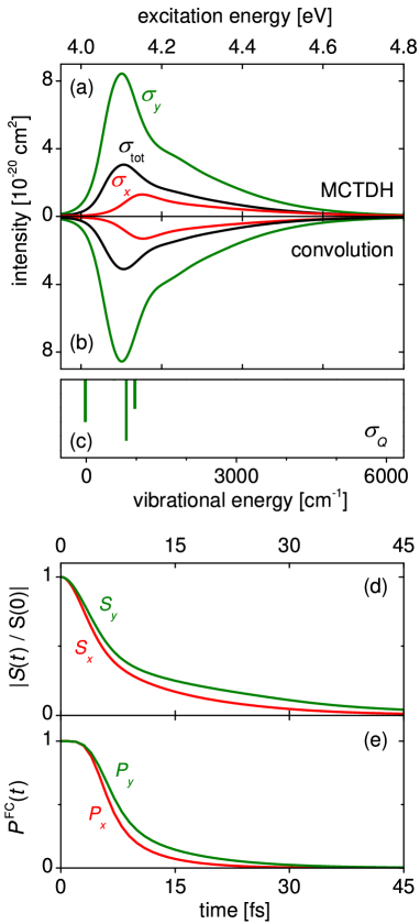
Figure 8: (a) Quantum mechanical absorption spectra for the isolated state ${}^{1}\!A_{2}$ in the 6D calculation. The profiles $\sigma_{x}$ (red), $\sigma_{y}$ (green), and the total absorption spectrum $\sigma_{\rm tot}$ (black) are shown. (b) The same spectra as in (a) evaluated using the convolution approximation. (c) The vibrational spectrum $\bar{\sigma}_{Q}$ used in the convolution. (d) The autocorrelation functions $|S_{x}|$ (red) and $|S_{y}|$ (green) versus time. (e) The populations in the FC region $P^{\rm FC}_{x}(t)$ (red) and $P^{\rm FC}_{y}(t)$ (green) as functions of time.

The spectra for the two polarizations, as well as the total absorption spectrum $(\sigma_{x}+\sigma_{y})/3$, are shown in Fig. 8(a). The total absorption maximum of about $3\cdot 10^{-20}\mbox{ cm}^{2}$ is reached at $E_{\mathrm{max}}=4.11$ eV, close to the vertical excitation energy of $T_{v}=4.19$ eV. Note that this $T_{v}$ is smaller than the value of 4.80 eV given in Table 2. The reason is the choice of the fixed values of the totally symmetric $a_{1}$ modes in this calculation: In the excitation zone, $\mathbf{Q}=\mathbf{Q}_{\mathrm{min}}(R)$ corresponds to the minimum of the state $1^{1}\!A_{2}(\pi\sigma^{*})$, but not of the state $\widetilde{X}$ which is elevated by $\sim 0.6$ eV. All spectra in Fig. 8(a) are composed of the main peak and the shoulder on the high energy side. The main peaks lie at $E_{\mathrm{max}}=4.15$ eV (for $\sigma_{x}$) and $E_{\mathrm{max}}=4.10$ eV (for $\sigma_{y}$), while the full widths at half maximum (FWHMs) are about 0.15 eV. The broad maxima in both components correspond to quasi-bound resonances supported by the local minimum of the potential $V^{A_{2}}$. The FWHM is determined by two factors, the number of the excited (mostly short lived) resonances and their linewidths. While the vibrational assignments are addressed below, one aspect of the excitation pattern follows directly from the molecular geometry. The N—H bond in the $1^{1}\!A_{2}(\pi\sigma^{*})$ is elongated by $0.12\,a_{0}$ relative to the state $\widetilde{X}$, and the local minimum of $V^{A_{2}}$ is shifted to larger $R$ distances. Correspondingly, the main peaks and the shoulders are built on zero quanta and one quantum of N—H stretch, respectively.

The maximum absorption for $\sigma_{y}$ is more than 8 times stronger than for $\sigma_{x}$, even though the Herzberg-Teller coefficients for the TDMs $\mu_{x}$ along the in-plane bending and $\mu_{y}$ along the out-of-plane bending modes are comparable (see Table 3). The intensity of $\sigma_{y}$ is large due to a subtle enhancement effect: The out-of-plane bending frequency is $\sim 3$ times smaller than the in-plane one, and the range of $\theta$ covered by the parent wave function $\Psi_{0}(\mathbf{R},\mathbf{Q}_{b_{1}})$ along the out-of-plane direction is about $\sim\sqrt{3}$ broader than along the in-plane direction. Consequently, the integrated TDM, sampled over an enhanced $\theta$ range, is larger by a factor of $\sim 3$, and the calculated intensity for $\sigma_{y}$ is amplified by $\sim 3^{2}$.

Using the low storage filter diagonalization, the main absorption peaks can be uniquely assigned to intense resonance states located at $E_{\mathrm{res}}=4.14$ eV (for $\sigma_{x}$) and at $E_{\mathrm{res}}=4.07$ eV and 4.11 eV (for $\sigma_{y}$). These energies correspond to one quantum excitations of the in-plane H-atom bend, the out-of-plane H-atom bend, and the ring mode $Q_{b_{1}}(3)$, respectively (corresponding frequencies are $0.13$ eV, $0.08$ eV, and $0.12$ eV, see Table 3). These modes have large Herzberg-Teller coefficients in Table 3, and their excitation is expected. Several short lived resonance states are found at energies correlating with the spectral shoulders and assigned to overtone excitations of the out-of-plane H-atom bend (for $\sigma_{y}$) and the combination bands involving one quantum of N—H stretch (for $\sigma_{x}$ and $\sigma_{y}$).

The lifetimes $\tau_{\rm res}$ of the resonances corresponding to the main peaks provide estimations of the quantum mechanical dissociation time scale. We find 5.6 fs for $\sigma_{x}$ and 8 fs for $\sigma_{y}$. These lifetimes are of the order of the shortest dissociation time $\tau_{d}=12$ fs measured in Ref. WNSSAWS15, (see Table 6). The calculated $\tau_{\rm res}$ is short indicating that the effective potential barrier in the FC region is not high enough to support tunneling regime. In Ref. WNSSAWS15, , this time scale was associated with the direct dissociation in the state $1^{1}\!A_{2}(\pi\sigma^{*})$, too.

Dissociation time scale can also be assessed using the autocorrelation functions $S_{\epsilon}(t)$ and the population in the inner potential region $P_{\epsilon}^{\mathrm{FC}}(t)$. They are depicted in Fig. 8(d,e). The autocorrelation functions for both polarizations decay monotonically without visible recurrences, and the exponential time constants of 7.5 fs (for $S_{x}$) and 9.5 fs (for $S_{y}$) are consistent with the resonance lifetimes. The populations in the FC zone [Eq. (24)] have a very short ‘induction’ plateau $T_{0}$, while the time scales for the direct and indirect contributions are almost equal: $T_{1}\approx T_{2}\approx 5.2$ fs (for $P_{x}^{\mathrm{FC}}$) and $T_{1}\approx T_{2}\approx 6.5$ fs (for $P_{y}^{\mathrm{FC}}$). This is yet another indication that tunneling contribution is small. In order to verify this conclusion, we estimate the isotope effect of the reaction,

$$KIE=\frac{\tau(D)}{\tau(H)}\,,$$ (32)

by substituting D for H in the N—H group (‘pyrrole-$d_{1}$’) and repeating the quantum mechanical calculations. Based on the resonance lifetimes as well as the survival probabilities, a modest isotope effect of about 2.5—3.5 is predicted. This confirms that tunneling does not significantly affect dissociation in the state $1^{1}\!A_{2}(\pi\sigma^{*})$, and the lowest barrier $E^{\ddagger}_{\rm MEP}$ in Table 1 is dynamically relevant. Roberts et al. studied the isotope effect in the photodissociation of pyrrole and found that the strength of the effect depends on the measured dissociation lifeimes: For $\tau_{d}=46$ fs, they found $KIE\sim 2.9$ which is close to our result; for a much longer lifetime of 126 fs, the measured $KIE$ is about 11.RWYCYUS13

Figure 8(b) shows the spectra calculated using the convolution approximation of Eq. (30) for each polarization separately. The agreement with the MCTDH calculations is excellent for all spectra. Comparison with calculations involving other pyrrolyl modes and described below suggests that the convolution is especially effective for the non-totally symmetric oscillators (like the $b_{1}$ modes) because their minima are not displaced in either $\widetilde{X}$ or $A_{2}$ states and they are to a large extent decoupled from the H-atom coordinates $\mathbf{R}$. As a result, the separable approximation of Eqs. (27) and (28) is accurate.

The two convolution factors $\bar{\sigma}_{R}$ and $\bar{\sigma}_{Q}$ [Eq. (29)] can be distinguished in the spectra. In the excitation via $\mu_{x}$, the initial vibrational wavefunction $f_{Q}(\mathbf{Q}_{b_{1}})$ overlaps only with the ground state of the pyrrolyl ring in the state $1^{1}\!A_{2}(\pi\sigma^{*})$. The discrete spectrum $\bar{\sigma}_{Q}$ (not shown) consists of a single peak, and the convoluted spectrum $\sigma_{x}$ in Fig. 8(b) coincides with the dissociative factor $\bar{\sigma}_{R}(E)$. For the $y$-polarized transition, the harmonic FC spectrum $\bar{\sigma}_{Q}$ includes several lines shown in Fig. 8(c). The position of $\bar{\sigma}_{Q}$ on the photon energy scale is chosen so that the vibrational states of the ring have correct excitation energies relative to the quantum mechanical band origin evaluated in the convolution approximation. The TDM $\mu_{y}$ depends on both the out-of-plane H bending and the $b_{1}$ modes (cf. Table 4). Consequently, three vibrational states make the largest contribution to $\bar{\sigma}_{Q}$: The ground vibrational state of the ring (accessed because the excitation resides on the out-of-plane H bending), as well as the ring states with one quantum on the modes $Q_{b_{1}}(2)$ or $Q_{b_{1}}(3)$. The Herzberg-Teller coefficient for the mode $Q_{b_{1}}(1)$ is small, and this mode is not excited. As expected, this assignment is consistent with one given for the resonance states. This is an illustration that the convolution method can be effectively used to automatically label vibrational peaks in electronic spectra. The convolution approximation confirms that the shoulder of the spectrum $\sigma_{y}$ is due to the same ring states combined with the overtone excitations of the disappearing modes. This spectral pattern — a given set of the ring quanta ‘translated’ to higher energy absorption bands via additional excitations of the N-H stretch or H bend — is a characteristic feature of the absorption spectrum of pyrrole.

IV.2 11D absorption spectrum: Coordinates $R,\theta,\phi,Q_{a_{1}}(1,2,3,4,5,6,7,8)$

In this calculation, all $a_{1}$ ring modes are included and all remaining non-totally symmetric pyrrolyl modes are fixed to the equilibrium values of $\mathbf{Q}={\bm{0}}$. As in the 6D case, the isolated state $1^{1}\!A_{2}(\pi\sigma^{*})$ is excited via the TDMs $\mu_{x}$ and $\mu_{y}$ (Table 4) giving the initial states $\Phi_{x}(0)$ and $\Phi_{y}(0)$ of $b_{2}$ and $b_{1}$ symmetry. Each TDM consists of only one term depending on the angular coordinates $(\theta,\phi)$ and representing the in-plane ($\mu_{x}$) and the out-of-plane ($\mu_{y}$) excitations of the H-atom bending in the state $1^{1}\!A_{2}(\pi\sigma^{*})$.

The total absorption spectrum $\sigma=(\sigma_{x}+\sigma_{y})/3$ and the spectra $\sigma_{x}$ and $\sigma_{y}$ are given in Fig. 9(a). Similarly to the 6D case, the absorption $\sigma_{x}$ (with the maximum of $6\cdot 10^{-21}\ \mathrm{cm}^{2}$) is almost an order of magnitude weaker than $\sigma_{y}$ (the maximum is $\sim 2.5\cdot 10^{-20}\ \mathrm{cm}^{2}$). For the total spectrum, the maximum intensity of $\sim 10^{-20}\ \mathrm{cm}^{2}$ is found at $E_{\mathrm{max}}=4.75$ eV, near $T_{v}=4.80$ eV. The vertical excitation energy in this calculation is the same as for the full 21D Hamiltonian in Table 2: With all totally symmetric modes included, the potential well of the 11D potential $V^{X}$ attains its global minimum, and the energy separation with the local minimum of $V^{A_{2}}$ is the largest. The distinct features against the 6D case are the diffuse structures superimposed on the $\sim 0.6$ eV broad background in the spectrum $\sigma_{y}$ (more pronounced) and in the total absorption (less pronounced). In Fig. 9(a), they are labeled with letters A—G. Their assignment, clarified below using the convolution method, reflects the principal geometry changes between the ground and the excited electronic state. The appropriate coordinates for such analysis are the normal modes $\widetilde{\mathbf{Q}}_{a_{1}}$ of the pyrrolyl ring at the local minimum of the potential $V^{A_{2}}$. These modes are used in the following discussion; they are numbered in order of their increasing frequency $\widetilde{\omega}$ (see Table 3). The stronger the shift $\delta Q$ of a particular mode between the minima of $V^{X}$ and $V^{A_{2}}$, the more overtones of this vibration are excited in the absorption spectrum. The largest dimensionless displacements $\delta Q$ are found for the modes $\widetilde{Q}_{a_{1}}(1)$ ($\widetilde{\omega}=908\,{\rm cm^{-1}}$, $\delta Q=0.54$), $\widetilde{Q}_{a_{1}}(2)$ ($\widetilde{\omega}=1124\,{\rm cm^{-1}}$, $\delta Q=1.32$), $\widetilde{Q}_{a_{1}}(3)$ ($\widetilde{\omega}=1155\,{\rm cm^{-1}}$, $\delta Q=1.03$), and $\widetilde{Q}_{a_{1}}(5)$ ($\widetilde{\omega}=1584\,{\rm cm^{-1}}$, $\delta Q=1.15$). Thus, several ring modes plus the dissociation coordinate $R$ have appreciable shifts, and several distinct vibrational progressions are expected in the 11D case. This is the reason why the overall width of the 11D spectra is about four times the width of the 6D spectra. The remaining modes $\widetilde{Q}_{a_{1}}(4,6,7,8)$ are minimally shifted, and behave as ‘spectators’.

Note that although many vibrational states are excited in both $\sigma_{x}$ and $\sigma_{y}$, the lines are considerably broadened by dissociation, and many members of the vibrational progressions remain unresolved. The broadening is more pronounced in the spectrum $\sigma_{x}$ rendering it smooth especially if compared to the structured spectrum $\sigma_{y}$: Dissociation of the in-plane excited wave packet is considerably faster than of the out-of-plane one. This is directly confirmed with the autocorrelation functions depicted in Fig. 9(d). Although both $S_{x}$ and $S_{y}$ rapidly decrease in the first several femtoseconds, the in-plane $S_{x}$ drops, relative to its value at $t=0$, by three orders of magnitude — 5 times more than $S_{y}$. The origin of this difference lies in the potential energy profiles of $V^{A_{2}}$ along the dissociation direction $R$ and along the polar angle $\theta$ for the H-atom moving in the state $1^{1}\!A_{2}(\pi\sigma^{*})$ perpendicular to pyrrolyl plane ($\phi=0^{\circ}$) and in the pyrrolyl plane ($\phi=90^{\circ}$). The contour plot in Fig. 4(a) is for $\phi=0^{\circ}$. The local minimum near $R=4.2\,a_{0}$, which is the deepest for $\theta=0^{\circ}$, persists for $\theta>0^{\circ}$, too. In fact, even H-atoms displaced by $\theta=40^{\circ}$ above the ring still experience a barrier to dissociation. For the in-plane motion ($\phi=90^{\circ}$; not shown in Fig. 4), the local minimum exists only for $\theta<10^{\circ}$, and no barrier hinders dissociation for larger in-plane displacements along $\theta$. As a result, the dissociation is direct and fast for the in-plane excitations ($\sigma_{x}$ in this case).

The dissociation time scale, prevailing near the absorption maximum, is established using the population in the inner potential region $P_{y}^{\mathrm{FC}}(t)$ shown in Fig. 9(e). The plateau region $T_{0}$ is of the order of 1 fs, the direct (Gaussian) decay proceeds with the time constant of $T_{1}=12.8$ fs and accounts for 80% of dissociating molecules, while the indirect exponential lifetime is $T_{2}=23.8$ fs and has a weighting factor of 20%. These time constants are also covered in the resonance spectrum obtained via filter diagonalization: Several intense resonance states are found in the vicinity of each diffuse structure in the spectrum $\sigma_{y}$, with the lifetimes ranging from 8 fs (for $E_{\mathrm{res}}=4.49$ eV) to 30 fs (for $E_{\mathrm{res}}=4.66$ eV). The potential $V^{A_{2}}$ also supports resonance states with lifetimes over 100 fs. Such states are detected with filter diagonalization at low excitation energies. However, their intensity is very small in our calculations, less than 10^-4 of the intensity of the short lived states, and they are not included in the analysis. The comparison with the experimental values is summarized in Table 6. The short time scale agrees with $\tau_{d}=12$ fs measuredWNSSAWS15 at $\lambda=242$ nm using the time-resolved photoelectron spectroscopy sensitive to the population of the excited state in the FC zone. The longer time constant is close to the value of $19$ fs from the same experiment, and also overlaps with the dissociation times of $\tau_{d}=39$ fs at $\lambda=249.5$ nm (Ref. KPNWF17, ; the time resolution of 3 fs) and 46 fs at $\lambda=238$ nm (Ref. RWYCYUS13, ; the time resolution of 30 fs).

The isotope effect is estimated using Eq. (32) in a separate quantum mechanical calculation of pyrrole-$d_{1}$. For the D-substituted molecule, the direct dissociation time $T_{1}$ increases only slightly, so that $KIE\approx 1.0$. The indirect time constant $T_{2}$ becomes 41.8 fs with $KIE\approx 1.8$, slightly smaller than in 6D. Tunneling might indeed contribute to the time constants longer than 20 fs, but this contribution tends to decrease as more degrees of freedom are added. Calculations of resonance states support this conclusion, and predict the isotope effect between 1.0 (for states with lifetimes of under 10 fs) to 2.5 (for lifetimes over 20 fs), although in the 11D case it is not always possible to uniquely match resonance states in pyrrole and in pyrrole-$d_{1}$. Again, the calculated $KIE$ is in close agreement with the experimental estimate given in Ref. RWYCYUS13, for similar lifetimes.

The autocorrelation functions in Fig. 9(d) suggest vibrational assignments in the time domain. In $|S_{y}|$, the shortest recurrence time of 21 fs corresponds to the frequency of about 1600 cm^-2 associated with the mode $\widetilde{Q}_{a_{1}}(5)$. Another broad recurrence of nearly the same intensity is seen around 35 fs. It is associated with low-frequency $a_{1}$ modes $\widetilde{Q}_{a_{1}}(1,2,3)$, which span the frequency range 900–1150 cm^-2. Based on this analysis and assuming that the band A in the spectrum $\sigma_{y}$ carries zero quanta in the ring modes, we expect to find vibrational states (i) with one quantum on $\widetilde{Q}_{a_{1}}(5)$ (e.g. near the shoulder C at $E_{\mathrm{ph}}=4.60$ eV) and (ii) with one quantum on $\widetilde{Q}_{a_{1}}(1,2,3)$ (e.g. near the band B peaking at $E_{\mathrm{ph}}=4.50$ eV). This is in line with the discussion based on shifts $\delta Q$ of normal modes in the initial and final electronic states.

Fig. 9(b) depicts the spectra $\sigma_{x}$ and $\sigma_{y}$, calculated using the convolution method. The resulting absorption profiles agree well with the exact MCTDH calculation: The convoluted spectra are correctly positioned on the energy scale and the moments of the spectral envelope (width, asymmetry, etc.) are well reproduced. The lower resolution of the $\sigma_{x}$ profile, compared to $\sigma_{y}$, is also correctly captured. On the other hand, the absorption bands in the convoluted spectrum $\sigma_{y}$ are slightly more pronounced than in its MCTDH counterpart. This indicates that the spectral broadening, represented by the factor $\bar{\sigma}_{R}$, is underestimated and the coupling between $\mathbf{Q}$- and $\mathbf{R}$-spaces is only approximately taken into account. In fact, the 11D calculation including all $a_{1}$ vibrational modes represents a stringent test for the method, because anharmonic coupling with the totally symmetric dissociation coordinate $R$ is symmetry-allowed, and for many $a_{1}$ modes this coupling is indeed strong.

In these calculations, the convolution factors $\bar{\sigma}_{R}$ exemplified in Fig. 9(c) consist of the main peak and several high energy shoulders, i.e. they are similar to those discussed in the 6D case. Their FWHMs of 0.18 eV (for $\mu_{x}$) and 0.12 eV (for $\mu_{y}$) also compare well with 6D. The spectrum $\bar{\sigma}_{R}$ is broader for the $x$-polarized case, indicating faster decay of the in-plane excitation, in agreement with the analysis given above in terms of the potential energy curves. The total spectral width of 0.6 eV is approximately four times larger than the width of $\bar{\sigma}_{R}$, so that most of the spectral broadening is due to the long $a_{1}$ progressions in the convolution factor $\bar{\sigma}_{Q}$ (FWHM of $\sim 0.4\,{\rm eV}$) shown in Fig. 9(c). In the calculation of $\bar{\sigma}_{Q}$, the value of the dissociation coordinate for the state $1^{1}\!A_{2}$ is fixed at $R_{\mathrm{FC}}=4.23\,a_{0}$. The vibrational ground state of the ring in the state $\widetilde{X}$ is taken at $R_{\mathrm{FC}}=4.10\,a_{0}$.

The sequence of vibrational peaks in the convoluted spectrum $\sigma_{y}$ is similar to the one found in the exact MCTDH spectrum. The intense peaks in the exact and the convoluted spectra are matched by visual inspection, and the corresponding bands are labeled with the same letters in Figs. 9(a) and (b). The same bands can be found in the total spectrum $\sigma_{\rm tot}$, too, albeit with smaller intensity. They can be unequivocally matched to the peaks in the harmonic convolution factor $\sigma_{Q}$ in Fig. 9(c). One advantage of the convolution method is that the constructed spectrum — like any other FC spectrum — is automatically assigned in terms of the ring modes, because each vibrational contribution to $\bar{\sigma}_{Q}$ [Eq. (31)] is known. In addition, the dissociative factor $\bar{\sigma}_{R}$ giving the band shape of each spike in $\bar{\sigma}_{Q}$ helps to identify the excitations of the disappearing modes in the absorption bands. Guided by the shape of the spectrum $\bar{\sigma}_{R}$, we distinguish to main groups of excitations contributing to a given band, one due to the lowest allowed (‘obligatory’) excitation of the disappearing modes and another involving overtone excitations in the $\mathbf{R}$-space. The first group is associated with the main peak in $\bar{\sigma}_{R}$, the second — with the shoulders. The assignments for the bands A—G corresponding to the first group are given in the caption to Fig. 9. The resulting assignments confirm the previous analyses based on the shifts $\delta Q$ and the autocorrelation function. Indeed, the most intense peaks involve excitations in the modes which are strongly displaced between the minima of $V^{X}$ and $V^{A_{2}}$, namely $\widetilde{Q}_{a_{1}}(2)$, $\widetilde{Q}_{a_{1}}(5)$, which give rise to the most intense progressions, and $\widetilde{Q}_{a_{1}}(3)$, which gives rise to slightly weaker peaks. The vibrational couplings between $R$ and the $a_{1}$ modes are neglected in the convolution method based on the separable approximation, and the vibrational frequencies do not perfectly coincide with those in the MCTDH calculation. For example, the band B, involving one quantum excitations on the modes $\tilde{Q}_{a_{1}}(2)$ and $\tilde{Q}_{a_{1}}(3)$, appears to be shifted to higher energies by $\sim 120\,{\rm cm}^{-1}$; the energy of the shoulder C, to which the mode $Q_{a_{1}}(5)$ contributes significantly, is underestimated by $\sim 130\,{\rm cm}^{-1}$.

The second group of excitations involving overtones of the disappearing modes can also be distinguished in many bands. One example is the normal vibrational ring state ${\bf 0}$ which, combined with the obligatory out-of-plane bending excitation $n_{\theta}=1$, provides the main assignment of the band A in the spectrum $\sigma_{y}$. The same ring state, augmented with two more bending quanta ($n_{\theta}=3$), contributes to the band B and, augmented with the NH stretch excitation ($n_{R}=1$), to the band D. Further, the ring excitations contributing to the band B are also found in the band D (with the $\mathbf{R}$-space excitation $n_{\theta}=3$). The ring states $n_{a1}(2)=1$, $n_{a1}(3)=1$, and $n_{a1}(5)=1$, dominating the band D, also contribute, via the additional excitation $n_{\theta}=3$ to the band F. In fact, most ring excitations listed in Fig. 9 are found in the higher lying absorption bands with $n_{\theta}>1$ and $n_{R}>0$. The energy stored in the disappearing modes during photoexcitation is expected to get released into rotations and translation in the course of dissociation.

IV.3 15D absorption spectrum: Coordinates $R,\theta,\phi,Q_{a_{1}}(1,2,5),Q_{a_{2}}(1,2,3),Q_{b_{1}}(1,2,3),Q_{b_{2}}(1,3,5)$

The third calculation discussed in this paper includes two coupled electronic states, $\widetilde{X}$ and $1^{1}\!A_{2}(\pi\sigma^{*})$. Three modes of each symmetry are dynamically active, in particular all symmetry-allowed coupling modes $Q_{a_{2}}(1,2,3)$ of the ring are included. All other modes are set to their equilibrium values for pyrrolyl. The excitation $1^{1}\!A_{2}\leftarrow\widetilde{X}$ is mediated by three TDM components $\mu_{x}$, $\mu_{y}$ and $\mu_{z}$. The initial states $\Phi_{x}(0)$, $\Phi_{y}(0)$, and $\Phi_{z}(0)$ (cf. Table 4) belong to the irreps $b_{2}$, $b_{1}$, and $a_{2}$, respectively. The states $\Phi_{x}(0)$ and $\Phi_{y}(0)$ are linear combinations of excitations of the disappearing modes $(\theta,\phi)$ and the one-quantum excitations of the ring. The state $\Phi_{z}(0)$ includes only the fundamental excitations of the ring modes $Q_{a_{2}}$.

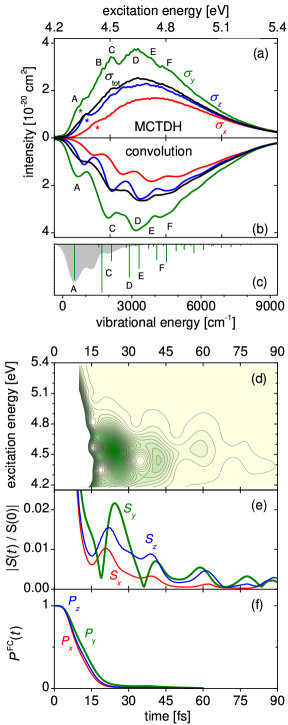
Figure 10: (a) Quantum mechanical absorption spectra for the coupled $1^{1}\!A_{2}/\widetilde{X}$ states in the 15D calculation. The components $\sigma_{x}$ (red), $\sigma_{y}$ (green), $\sigma_{z}$ (blue), and the total absorption spectrum $\sigma_{\rm tot}$ (black) are shown. (b) The same spectra evaluated using the convolution approximation. (c) The ‘spectra’ $\bar{\sigma}_{Q}$ (sticks) and $\bar{\sigma}_{R}$ (gray shade) used in the convolution. (d) The spectrogram $S_{y}(E,\tau)$ as defined in Eq. (33). (e) The autocorrelation functions $|S_{x}|$ (red), $|S_{y}|$ (green) and $|S_{z}|$ (blue) versus time. (f) The populations in the FC region $P^{\rm FC}_{x}(t)$ (red), $P^{\rm FC}_{y}(t)$ (green) and $P^{\rm FC}_{z}(t)$ as functions of time. In (c) and (d), the results for the $y$-polarized excitation induced by the TDM $\mu_{y}(\mathbf{R})$ are shown. The vibrational bands marked with letters A–F in (a) and (b) are assigned in terms of the quantum numbers $n_{\Gamma}(i)$ belonging to the irrep $\Gamma$. The states mostly contributing to each $\sigma_{y}$ peak are: (A) $n_{a_{1}}(i)=0$, $n_{b_{1}}(2)=1$, $n_{b_{1}}(3)=1$, and the fundamental excitation of the out-of-plane H bending; (B) the states of the band A with $n_{a1}=1$; (C, D) the states of the band A with $n_{a_{1}}(2)=1$, with $n_{a_{1}}(5)=1$, with $n_{a_{1}}(2)=2$, as well as with the combination states $(n_{a_{1}}(2)=1,n_{b_{1}}(2)=1)$ and $(n_{a_{1}}(2)=1,n_{b_{1}}(3)=1)$; (E) the states in A with $(n_{a_{1}}(2)=1,n_{a_{1}}(5)=1)$; (F) the states in A with $n_{a_{1}}(2)=3$, and with $(n_{a_{1}}(2)=2,n_{a_{1}}(5)=1)$. The listed ring excitations are accompanied by the ‘obligatory’ excitations of the disappearing modes.

The spectra for the individual polarizations and the total spectrum $\sigma=\left(\sigma_{x}+\sigma_{y}+\sigma_{z}\right)/3$ are shown in Fig. 10(a). As in all preceding calculations, the absorption $\sigma_{y}$ is the strongest (the maximum intensity is $3.7\cdot 10^{-20}\,{\rm cm}^{2}$). It is about 2 times more intense than the weakest spectrum $\sigma_{x}$ (the maximum is $1.7\cdot 10^{-20}\,{\rm cm}^{2}$). The contribution $\sigma_{z}$, absent in the 6D and 11D calculations, is intermediate between the two, with the peak intensity of $2.3\cdot 10^{-20}\,{\rm cm}^{2}$. The total absorption reaches the maximum at 4.70 eV, and the FWHM of the absorption envelope is 0.61 eV. These main absorption parameters are in good agreement with the 11D calculation. In particular, the true minimum of $V^{X}$ as well as the principal geometrical changes between $V^{X}$ and $V^{A_{2}}$ — which are controlled by the totally symmetric modes — are accurately described by the three included modes $Q_{a_{1}}(1,2,5)$. Further, all non-totally symmetric modes with large Herzberg-Teller coefficients in the TDM are also included, so that the maximum total intensity of $2.5\cdot 10^{-20}\,{\rm cm}^{2}$ is expected to be accurate. The 15D calculation is our most reliable estimate of the absorption spectrum of the state $1^{1}\!A_{2}(\pi\sigma^{*})$. It illuminates one of the intrinsic features of the $\pi\sigma^{*}$ photochemistry of model biochromophores: The total spectra of the $\pi\sigma^{*}$ states result from the contributions of several — in this case three — absorptions due to different spatial components of the TDM vector.

The broad absorption background is structured by several broad diffuse bands marked with letters A—F in Fig. 10(a). They are most conspicuous in the spectrum $\sigma_{y}$, and even there they are less pronounced than the vibrational bands in the 11D calculation. The marked bands are assigned below using the convolution method.

There is also a second group of absorption lines in all spectra in Fig. 10(a). They are narrow, densely spaced, and seen as ‘ripples’ on the spectral profiles. These bands have vibronic origin: They are found only for the coupled states $A_{2}/\widetilde{X}$ whereas the spectrum of the isolated state $1^{1}\!A_{2}(\pi\sigma^{*})$ is smooth. The narrow ‘ripples’ in Fig. 10(a) are Fano resonances which are due to the interference of two diabatic dissociation pathways, the direct dissociation pathway in the $A_{2}$ state and the indirect one involving vibronic transitions to the state $\widetilde{X}$ and back to $A_{2}$ at the CI $\widetilde{X}/^{1}\!A_{2}$. In fact, the ‘ripples’ are associated with the bound vibrational states of the state $\widetilde{X}$ which gain intensity via the CI. This interference, which has a strong impact on the $\pi\sigma^{*}$ photochemistry of pyrrole and affects the spectra and the photofragment distributions, has been analyzed in Ref. GP17A, .

The Fano effect is especially pronounced in the dynamics of the second excited state $1^{1}\!B_{1}(\pi\sigma^{*})$. For the state $1^{1}\!A_{2}(\pi\sigma^{*})$, discussed in this paper, the coupling at the CI is weak (the population transfer between $A_{2}$ and $\widetilde{X}$ is less than 10%) and the diffuse bands A—F are not affected by the state crossing and can be analyzed in terms of the state $1^{1}\!A_{2}(\pi\sigma^{*})$ alone. The lowest vibrational states excited in the spectra $\sigma_{x}$, $\sigma_{y}$, and $\sigma_{z}$ and marked with asterisks in Fig. 10(a) are associated with one quantum excitations in the vibrations promoting the $1^{1}\!A_{2}\leftarrow\widetilde{X}$ transition. The largest Herzberg-Teller coefficients are carried by the mode $\widetilde{Q}_{b_{2}}(3)$ (for $\sigma_{x}$; $\omega=1321\,{\rm cm}^{-1}$), the out-of-plane bending $\theta$ (for $\sigma_{y}$; $\widetilde{\omega}=616\,{\rm cm}^{-1}$), and the mode $\widetilde{Q}_{a_{2}}(3)$ (for $\sigma_{z}$; $\widetilde{\omega}=969\,{\rm cm}^{-1}$). The energies of the absorption origins are arranged according to the indicated frequencies of the isolated $A_{2}$ state, i.e. $E_{y}<E_{z}<E_{x}$. Moreover, the absorption maxima in the three spectra follow the same order: The larger the frequency of the mode promoting the transition, the higher the energy of the absorption maximum. In the following, we concentrate on the diffuse vibrational bands in the spectrum $\sigma_{y}$ which are strong and which also have clear counterparts in the total absorption spectrum. However, even this relatively simple spectrum is composite and consists of two contributions, the major one stemming from the excitation of the disappearing modes via the TDM $\mu_{y}(\mathbf{R})$ and the weak excitation of the ring via $\mu_{y}(\mathbf{Q})$.

Photodissociation in the 15D calculation is a fast process. In particular, the autocorrelation functions $S_{\epsilon}(t)$, shown in Fig. 10(e), decay over two orders of magnitude within $\sim 10$ fs. Much of this decay is due to the direct dissociation. This is confirmed with the time dependent survival probabilities $P_{\epsilon}^{\mathrm{FC}}(t)$ in panel (f). For the most intense $y$-polarized excitation, about 95% of all molecules dissociate directly with the time constant $T_{1}=11.7$ fs which is almost identical with the 11D calculation. The remaining 5% dissociate indirectly with the exponential lifetime of $T_{2}=36.0$ fs, which is somewhat longer than in the 11D case. These time constants can be cross validated using the resonance lifetimes: The resonance states corresponding to the diffuse bands A and F have longer lifetimes of 24 fs and 30 fs, respectively, while the intense resonance states found under the bands C and D are short lived, with $\tau_{\rm res}(l)<10$ fs (see Table 6). The theoretical time scales are slightly better aligned with the experimental values than in the low dimensional calculations. In particular, the correlations between $T_{1}$ and $\tau_{d}=12$ fsWNSSAWS15 and between $T_{2}$ and $\tau_{d}=46$ fsRWYCYUS13 become more apparent. Note that the resonance lifetimes, as well as the measured lifetimes collected in Table 6, are non monotonic functions of the photon energy. Such fluctuations are often encountered and well understood in small polyatomic molecules.GSCHH03 The lifetimes fluctuate because eigenstates excited along different vibrational modes experience different effective coupling to the continuum. The observation of the lifetime fluctuations in pyrrole can therefore be a signature of the state- or even mode specific photodissociation in this biochromophore.

The isotope effect in pyrrole-$d_{1}$ is evaluated using the populations $P_{y}^{\mathrm{FC}}(t)$. The resonance states are not used because it becomes nearly impossible to reliably match the resonance energies in two molecules. The isotope effect in the 15D case follows the trend of the lower dimensional calculations. The direct dissociation time in pyrrole-$d_{1}$ is $T_{1}=13.0$ fs giving $KIE\approx 1.1$. The indirect time is 55.4 fs so that in this case $KIE\approx 1.54$. As expected, the isotope effect diminishes with increasing dimensionality, and the tunneling contribution is not very significant.

Recurrences in the autocorrelation functions in Fig. 10(e) help to analyze the vibrational structure of the spectrum. Three short time recurrences are seen in $S_{y}(t)$ followed by a series of less regular weak peaks stretching over several hundred femtoseconds [not shown in panel (e)]. The strong short time recurrences are responsible for the main absorption peaks A—F while the weak ones are associated with the long lived Fano resonancesGP17A which are beyond the scope of the present discussion. The relation between the recurrence times and the absorption bands can be conveniently visualized using the so-called spectrogram

$$S_{y}(E,\tau)=\int S_{y}(t)h(t-\tau)e^{iEt}\,dt\,,$$ (33)

which is a moving window Fourier transform of the autocorrelation function. Here $h(t)=\exp(-t^{2}/2t_{0}^{2})$ is the Gaussian window function. In the spectrogram $S_{y}(E,\tau)$, shown in Fig. 10(d), the time and the frequency domains are represented in the same plot at the expense of the resolution which is smeared along both axes:JK89 ; HHG95 ; VVS96 The time resolution $t_{0}$ in the plot is 5 fs and corresponds to the energy resolution of $\hbar/t_{0}=1100$ cm^-1. The spectrogram is dominated by three maxima. The largest maximum is found at $\tau=24$ fs and $E_{\rm ph}=4.50$ eV. The energy is close to that of the band C which can thus be associated with excitations of frequency $\omega\approx 2\pi/\tau\sim 1350$ cm^-1. Several vibrational modes have fundamentals or overtones close to this frequency, e.g. one quantum of the totally symmetric mode $\widetilde{Q}_{a_{1}}(2)$ or the out-of-plane bending mode. A two quantum excitation of $\widetilde{Q}_{b_{1}}(2)$ could be another possibility, but this non-totally symmetric mode has a zero equilibrium shift $\delta\widetilde{Q}$ and a tiny frequency change between the ground and the excited electronic states; its excitation is therefore unlikely. The largest maximum in the spectrogram extends over an appreciable energy range. With growing energy the recurrence time becomes shorter so that around 4.62 eV (band D) $\tau\sim 21$ fs correlates well with the frequency of $\widetilde{Q}_{a_{1}}(5)$. The other two maxima in the spectrogram are more localized in energy. One, seen at $\tau=42$ fs and $E_{\rm ph}=4.42$ eV, lies close to the band B, and the associated frequency is $\sim 800$ cm^-1. One quantum of $\widetilde{Q}_{a_{1}}(1)$ or a two quantum excitation of the non-totally symmetric mode $\widetilde{Q}_{b_{1}}(1)$ can account for this frequency. The other maximum is found at $\tau=60$ fs and $E_{\rm ph}=4.58$ eV, in the vicinity of the broad band D. The corresponding frequency of merely 560 cm^-1 is too small to be related to any pure excitation. More likely is that this low frequency is associated with a quantum beat between two surviving resonance states. A state with one quantum along $\widetilde{Q}_{a_{1}}(5)$ and a state with two quanta along $\widetilde{Q}_{b_{1}}(1)$ is an example of such a pair.

The quantum mechanical spectra calculated using MCTDH are compared with the convolution approximation in Fig. 10(b). The convolution is applied to the single state $A_{2}$, and the spectrum constructed using the convolution factors $\bar{\sigma}_{R}$ and $\bar{\sigma}_{Q}$ describes the diffuse vibrational bands but not the Fano resonances. Because the TDMs $\mu_{x}$ and $\mu_{y}$ are sums of two terms depending on the coordinates of $\mathbf{R}$- and $\mathbf{Q}$-space, two convolution terms are needed to approximate the spectra $\sigma_{x}$ and $\sigma_{y}$, as shown in Appendix B. The ‘spectrum’ $\bar{\sigma}_{R}$, exemplified in 10(c) for the initial state $\Phi_{y}(0)$, consists of the main peak and a series of satellites arising as in the 11D case from the additional excitations of the disappearing H atom bending ($n_{\theta}>0$) and NH stretch ($n_{R}>0$). The widths of $\bar{\sigma}_{R}$ and $\bar{\sigma}_{Q}$ are $\sim 0.15\,{\rm eV}$ and $\sim 0.4\,{\rm eV}$, respectively: As in the 11D case, the total width of 0.65 eV is mainly due to the progression in the ring modes of $a_{1}$ symmetry, whereas the dissociation induces a smaller broadening.

The convolution approximation correctly captures the shapes of the quantum mechanical absorption spectra, especially the low resolution envelopes. The intensities of the diffuse bands are clearly overestimated, especially for the spectra $\sigma_{x}$ and $\sigma_{z}$. As in 11D, the lack of anharmonic coupling leads to more narrow and better resolved bands. On the other hand, the approximation correctly reproduces the differences in the spectral resolution between the polarizations, and returns $\sigma_{y}$ as the most structured and $\sigma_{x}$ as the least structured spectrum.

The bands in the convolution and in the MCTDH spectra can be matched and related to the vibrational states in the local $A_{2}$ minimum. The assignment of this high dimensional spectrum is by no means straightforward, and we concentrate on the spectrum $\sigma_{y}$ again. The convolution reproduces all major bands, only the weak band B appears to be missing. This band is probably associated with the excitation of the $Q_{a_{1}}(1)$ mode which is highly correlated with the Jacobi coordinate $R$ and therefore is not well described by the convolution approach. The vibrational states of the pyrrolyl ring contributing to the bands A—F and and accompanied by the obligatory excitations in the $\mathbf{R}$-space are summarized in the caption to Fig. 10.

The band origin A includes the vibrational states with one quantum of excitation in the out-of-plane bending and the ring modes of $b_{1}$ symmetry. The vibrational states contributing to the bands ${\rm B}-{\rm F}$ belong to several progressions involving excitations out of the band origin. Most of the vibrational activity registered in the convolution approximation is due to the ring modes $Q_{a_{1}}(2)$ and $Q_{a_{1}}(5)$. We find up to three quanta of excitation in $Q_{a_{1}}(2)$ and up to two quanta in $Q_{a_{1}}(5)$. This is in agreement with the above analysis of the spectrogram, and with the assignment of the corresponding bands in the convolution factor $\bar{\sigma}_{Q}$ in panel (c). The strong bands C and D mainly involve the states with one and two quanta of the totally symmetric modes $Q_{a_{1}}(2)$ and $Q_{a_{1}}(5)$, plus a contribution of the out-of-plane bending overtone. The weaker neighboring band E is also due to excitations in $Q_{a_{1}}(2)$ complemented with $Q_{a_{1}}(5)$. Higher excitations in these modes contribute to the band F.

As in the 11D spectrum, the ring states are transposed to the higher energy absorption bands via the additional excitations of the disappearing modes. An example is the state $n_{a_{1}}=1$ providing the main assignment of the band B. With an additional bending excitation, this state contributes to the band C. This general property of the absorption bands of pyrrole acquires significance in the analysis of the wavelength resolved distributions of the final states of the pyrrolyl radical: Absorption bands based on the same ring states and differing only in the extent of excitation of the disappearing modes tend to produce repetitive patterns in the photofragment distributions discussed in paper II and observed in experiment.

V Conclusions

This paper analyzes the photodissociation mechanisms of pyrrole promoted into the lowest excited $1^{1}\!A_{2}(\pi\sigma^{*})$ state. The focus is on the absorption spectrum and the dissociation lifetimes. The summary our main findings is as follows:

1. New 24 dimensional diabatic potential energy matrices of the ground electronic state $\widetilde{X}$ and the two lowest $\pi\sigma^{*}$ states are calculated using CASPT2 method and a local diabatization at conical intersections. Additionally, the coordinate dependent transition dipole moments necessary for the adequate description of the excitation process into dark electronic states are provided. The full dimensional Hamiltonian for the H-atom abstraction from the NH moiety attached to the pyrrolyl ring is constructed and used in the quantum mechanical MCTDH calculations of the photodissociation.

2. The ab initio calculations reproduce the known benchmarks for the excitation of the $\pi\sigma^{*}$ states in pyrrole with reasonable accuracy. The quantum mechanical calculations using 15 degrees of freedom predict the absorption of the state $1^{1}\!A_{2}(\pi\sigma^{*})$ to reach the maximum of $\sim 3\cdot 10^{-20}$ cm² near the photon energy of 4.70 eV.

3. The absorption spectra, including contributions due to different TDM components, are mildly structured, and the diffuse bands can be assigned to vibrational excitations belonging mainly to the pyrrolyl ring combined with excitations of the disappearing modes. The prominent diffuse structures are due to the resonance states supported by the shallow local minimum of the state $1^{1}\!A_{2}(\pi\sigma^{*})$.

4. The calculated dissociation lifetimes, which range from $\sim 12$ fs for the (major) direct decay component to $\sim 36$ fs for the (minor) indirect component, are in good agreement with the experimental observations. Resonance calculations explain the experimentally observed non monotonic dependence of the lifetime on the excitation energy as a signature of fluctuations due to the state specific photodissociation in pyrrole. Resonance states with lifetimes of over 100 fs are also found, but their intensity is very low in the calculations.

5. The kinetic isotope effect, evaluated for the pyrrole-$d_{1}$, is small, $KIE\leq 2.0$, and the tunneling contribution to the indirect dissociation is minor. This is because of the low barrier along the minimum energy path in the state $1^{1}\!A_{2}(\pi\sigma^{*})$.

6. For the calculations of the two coupled electronic states $\widetilde{X}$ and $1^{1}\!A_{2}(\pi\sigma^{*})$, numerous Fano resonances are found even for 15 dynamically active degrees of freedom illustrating the robustness of the Fano interference in pyrrole.GP17A

7. A computationally efficient approximation method to calculate the absorption spectra is introduced which represents the total absorption as a convolution of the structureless spectrum due to direct dissociation and the Franck-Condon stick spectrum of the pyrrolyl ring modes. The convolution approximation extends the familiar Franck-Condon approach to the case of dissociating molecules. The approximation works best for the contributions of the non-totally symmetric ring modes which have zero displacements between the ground and the excited electronic state. The largest deviations are found for the progressions in the totally symmetric ring modes (irrep $a_{1}$), but even in this case the main features of the quantum mechanical spectra of pyrrole are faithfully reproduced. The convolution approximation allows one to generate absorption spectra of dissociating molecules with a minimum ab initio input, and is also an efficient tool to automatically assign the diffuse vibrational bands.

Appendix A Quasi-diabatization based on the adiabatic Hessian matrices

In this Appendix we describe the procedure to obtain the diabatic states $\widetilde{X}$, $A_{2}$ and $B_{1}$ in the $\mathbf{Q}$-space. We specialize the discussion to the definition of the diabatic coupling for the $X/A_{2}$ conical intersection. A similar procedure is applied to the $X/B_{1}$ intersection.

In the $\mathbf{Q}$-space, the $X/A_{2}$ diabatic coupling is linear in the three normal modes of $a_{2}$ symmetry [cf. Eq. (5)]:

$$W_{Q}^{XA_{2}}(\mathbf{Q}|R)=\sum_{i=1}^{3}\lambda_{i}^{XA_{2}}(R)Q_{a_{2}}(i)\ ,$$ (34)

where the $R$-dependent coupling strength is given by the Eq. (6)

$$\lambda_{i}^{XA_{2}}(R)=\lambda_{{\rm CI},i}^{XA_{2}}\exp\left(-\left|\frac{R-R_{\rm CI}^{XA_{2}}}{\Delta}\right|^{n}\right)\ .$$ (35)

The diabatization involves the evaluation of five parameters ($\Delta$, $n$ and three pre-factors $\lambda_{{\rm CI},i}^{XA_{2}}$) and the calculation of the $R$-dependent diabatic Hessian matrices $\left\{\gamma^{\alpha}_{ij}(R)\right\}$ in terms of the ab initio adiabatic Hessians $\left\{\widetilde{\gamma}^{\alpha}_{ij}(R)\right\}$ ($\alpha=X,A_{2}$):

$$\gamma^{X}_{ij}(R)=\widetilde{\gamma}^{X}_{ij}(R)+2\frac{\lambda_{i}^{XA_{2}}(R)\lambda_{j}^{XA_{2}}(R)}{U_{\mathrm{Relax}}^{X}(R)-U_{\mathrm{Relax}}^{A_{2}}(R)}$$ (36a)

$$\gamma^{A_{2}}_{ij}(R)=\widetilde{\gamma}^{A_{2}}_{ij}(R)-2\frac{\lambda_{i}^{XA_{2}}(R)\lambda_{j}^{XA_{2}}(R)}{U_{\mathrm{Relax}}^{X}(R)-U_{\mathrm{Relax}}^{A_{2}}(R)}\ .$$ (36b)

In the main text, $\gamma^{\alpha}_{ij}(R)$ are denoted $\left.\gamma^{\alpha}_{\Gamma,ij}(R)\right|_{\rm dia}$, and $\widetilde{\gamma}^{\alpha}_{ij}(R)$ are denoted $\left.\gamma^{\alpha}_{\Gamma,ij}(R)\right|_{\rm adia}$. In Eq. (36b), the one-dimensional profiles $U_{\mathrm{Relax}}^{X}(R)$ and $U_{\mathrm{Relax}}^{A_{2}}(R)$ are evaluated on the MEP of the $1^{1}\!A_{2}$ state. At the geometries of the MEP, the adiabatic and diabatic energies coincide (up to reordering) whereas the adiabatic and diabatic Hessians with respect to the $a_{2}$ modes are different. The $R$-dependent Hessians $\left\{\widetilde{\gamma}^{X}_{ij}(R)\right\}$ and $\left\{\widetilde{\gamma}^{A_{2}}_{ij}(R)\right\}$ for the adiabatic states $\widetilde{X}$ and ${}^{1}\!A_{2}$, calculated at the geometries of the MEP, diverge in the proximity of the $X/A_{2}$ intersection, located at $R_{\rm CI}^{XA_{2}}=5.57\,a_{0}$. The diabatic Hessians $\left\{{\gamma}^{X}_{ij}(R)\right\}$ and $\left\{{\gamma}^{A_{2}}_{ij}(R)\right\}$ are constructed by requiring that they are finite and smooth as functions of $R$. This implies that the singularity of the adiabatic Hessians near the intersection is compensated by the divergent term $\sim 2\lambda_{i}\lambda_{j}/\left(U^{X}-U^{A_{2}}\right)$ of Eq. (36b).

In order to find the pre-factors $\lambda_{i}^{XA_{2}}(R)$, we combine Eq. (36a) and (36b):

$$-\frac{1}{4}\Delta\widetilde{\gamma}_{ij}(R)\Delta U(R) = -\frac{1}{4}\left(\widetilde{\gamma}^{X}_{ij}(R)-\widetilde{\gamma}^{A_{2}}_{ij}(R)\right)\left(U^{X}_{\mathrm{Relax}}(R)-U^{A_{2}}_{\mathrm{Relax}}(R)\right)$$

$$= \lambda^{XA_{2}}_{i}(R)\lambda^{XA_{2}}_{j}(R)-\frac{1}{4}\left({\gamma}^{X}_{ij}(R)-{\gamma}^{A_{2}}_{ij}(R)\right)\left(U^{X}_{\mathrm{Relax}}(R)-U^{A_{2}}_{\mathrm{Relax}}(R)\right)\ .$$

Since the diabatic Hessians are non-divergent, the parameters $\lambda_{{\rm CI},i}^{XA_{2}}$ are obtained by the limit

$$-\lim_{R\rightarrow R_{\rm CI}^{XA_{2}}}\frac{\Delta\widetilde{\gamma}_{ij}(R)\Delta U(R)}{4}=\lambda^{XA_{2}}_{{\rm CI},i}\lambda^{XA_{2}}_{{\rm CI},j}\ ,$$ (38)

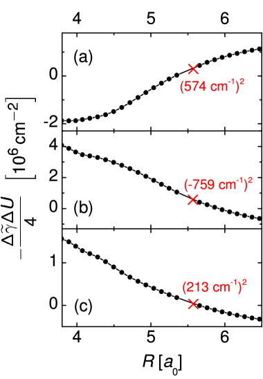
Figure 11: The quantities $-\Delta\widetilde{\gamma}_{ii}\Delta U/4$ of Eq. (LABEL:DgDV) (for $i=j$) calculated for the $a_{2}$ modes along the MEP on the $1^{1}\!A_{2}$ state. The plots of panels (a), (b) and (c) are obtained by using the diagonal adiabatic Hessian matrix elements $\widetilde{\gamma}^{\alpha}_{ii}$ for the modes $Q_{a_{2}}(1)$, $Q_{a_{2}}(2)$ and $Q_{a_{2}}(3)$, respectively. The red cross indicates the position of the conical intersection, where $-\Delta\widetilde{\gamma}_{ii}\Delta U/4=\left(\lambda_{{\rm CI},i}^{XA_{2}}\right)^{2}$. The values of $\lambda_{{\rm CI},i}^{XA_{2}}$ are reported in red.

which is evaluated by interpolating the quantities $-\Delta\widetilde{\gamma}_{ij}(R)\Delta U(R)/4$ calculated at the grid points of the MEP. Figure 11 shows the diagonal terms $-\Delta\widetilde{\gamma}_{ii}(R)\Delta U(R)/4$ as functions of $R$. Their values at the intersection are marked with red crosses and correspond to the squares of the coupling strengths at the intersection. The relative signs of the coupling strengths $\lambda_{{\rm CI},i}^{XA_{2}}$ are found by checking the signs of the off-diagonal terms $-\Delta\widetilde{\gamma}_{ij}(R)\Delta U(R)/4$ at $R=R_{\rm CI}^{XA_{2}}$.

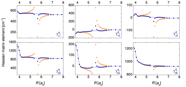
Figure 12: Adiabatic (orange dots) and diabatic (blue dots) Hessian matrix elements for the $1^{1}\!A_{2}$ electronic state with respect to the $a_{2}$ modes, calculated at the geometries of the MEP on the $A_{2}$ surface. The continuous blue line depicts the Hessian functions used in the wave packet calculations.

Once the pre-factors $\lambda_{{\rm CI},i}^{XA_{2}}$ are calculated, the parameters $\Delta$ and $n$ are tuned ‘by eye’, in order to obtain a smooth $R$-dependence of the diabatic Hessians, which are calculated using Eq. (36b). Figure 12 compares the adiabatic (orange dots) and the diabatic (blue dots) Hessian matrix elements for the $1^{1}\!A_{2}$ state along $R$. The diabatization removes the singularity of the ab initio adiabatic Hessian to a good extent. The resulting diabatic Hessian matrix elements vary smoothly with respect to $R$, except for a $0.5\,a_{0}$-wide strip around the intersection. The diabatic Hessians $\left\{\gamma^{X}_{ij}\right\}$ and $\left\{\gamma^{A_{2}}_{ij}\right\}$ are evaluated for a set of geometries of the MEP and interpolated for use in quantum mechanical calculations. Three points closest to the intersection are not included in the interpolation.

Appendix B Convolution approximation for a general form of the Herzberg-Teller TDM

In this Appendix, the convolution approximation described in Section III.2 is developed for a more general TDM function,

$$\mu(\mathbf{R},\mathbf{Q})=\sum_{i}\mu_{R,i}(\mathbf{R})\mu_{Q,i}(\mathbf{Q})\ ,$$ (39)

which includes Eqs. (17a)-(17b) as special cases.

The initial state of the parent molecules is taken as in Eq. (25), $\Psi_{0}(\mathbf{R},\mathbf{Q})\approx\Psi_{R}(\mathbf{R})\Psi_{Q}(\mathbf{Q})$, and the photoexcited state $\Phi(\mathbf{R},\mathbf{Q})$ is obtained by applying the TDM function of Eq. (39),

$$\Phi(\mathbf{R},\mathbf{Q}) = \mu(\mathbf{R},\mathbf{Q})\Psi_{0}(\mathbf{R},\mathbf{Q})$$ (40)

$$= \sum_{i}\left(\mu_{R,i}(\mathbf{R})\Psi_{R}(\mathbf{R})\right)\left(\mu_{Q,i}(\mathbf{Q})\Psi_{Q}(\mathbf{Q})\right)$$

$$= \sum_{i}F_{R,i}(\mathbf{R})f_{Q,i}(\mathbf{Q})\ .$$

Equation (40) is a generalization of the simple initial state of Eq. (26).

Using the separability approximation of Eq. (27) for the molecular Hamiltonian, an expression akin to Eq. (28) is obtained for the autocorrelation function:

$$S(t) \approx \sum_{ij}\left\langle F_{R,i}\left|\exp\left(-i\hat{H}_{R}t\right)\right|F_{R,j}\right\rangle_{R}\left\langle f_{Q,i}\left|\exp\left(-i\hat{H}_{Q}t\right)\right|f_{Q,i}\right\rangle_{Q}$$ (41)

$$= \sum_{ij}s_{R}^{ij}(t)s_{Q}^{ij}(t)\ .$$

where the cross correlation functions $s_{R}^{ij}(t)$ and $s_{Q}^{ij}(t)$ are built using the expansion terms $i$ and $j$ in Eq. (40). They are used to define the spectral functions

$$\bar{\sigma}_{R}^{ij}(E) = \int_{-\infty}^{\infty}s_{R}^{ij}(t){\rm e}^{iEt}{\rm d}t$$

$$\bar{\sigma}_{Q}^{ij}(E) = \int_{-\infty}^{\infty}s_{Q}^{ij}(t){\rm e}^{iEt}{\rm d}t\ .$$ (42)

The absorption spectrum, given by the Fourier transform of the autocorrelation function of Eq. (41), is finally given as

$$\sigma(E_{\mathrm{ph}})=\frac{E_{\mathrm{ph}}}{2\epsilon_{0}c}\sum_{ij}\int_{-\infty}^{\infty}\bar{\sigma}_{R}^{ij}(E_{\mathrm{ph}}-\omega)\bar{\sigma}_{Q}^{ij}(\omega){\rm d}\omega\ .$$ (43)

Eq. (43) is the extension of the convolution approximation to the TDM in the general form of Eq. (39).

The calculations of the contributions stemming from the $\mathbf{R}$- and $\mathbf{Q}-$spaces are performed separately. The initial functions $F_{R,i}(\mathbf{R})$ are propagated in the $\mathbf{R}$-space under the action of the Hamiltonian $\hat{H}_{R}$ and used to evaluate the cross-correlation functions $s_{R}^{ij}(t)$ whose Fourier transform gives the spectral functions $\bar{\sigma}_{R}^{ij}(E)$. The spectral functions $\bar{\sigma}_{Q}^{ij}(E)$ for the harmonic Hamiltonian $\hat{H}_{Q}$ are given by the expression akin to Eq. (31):

$$\bar{\sigma}_{Q}^{ij}(E)=\sum_{\bm{m}}\left.\left\langle f_{Q,i}(\mathbf{Q})\right|\phi_{\bm{m}}(\mathbf{Q})\right\rangle\left\langle\phi_{\bm{m}}(\mathbf{Q})\left|f_{Q,j}(\mathbf{Q})\right\rangle\right.\delta(E-E_{\bm{m}})\ ,$$ (44)

and depend on the analytic FC overlap integrals $\left\langle f_{Q,i}(\mathbf{Q})|\phi_{\bm{m}}(\mathbf{Q})\right\rangle$ for the ring modes.

Table 1: Properties of the CASPT2 potential energy surfaces of the three lowest electronic states of pyrrole compared with the available experimental data: Band origins $T_{0}$ which include zero-point energies of the ground and the excited electronic states; the quantum mechanical thresholds $D_{0}$ for the diabatic electronic channels; the potential barrier heights for the MEP, $E^{\ddagger}_{\rm MEP}$, and for the ring modes fixed to pyrrole equilibrium, $E^{\ddagger}_{\rm pyr}$. All energies are in eV.

Diabatic state	$T_{0}$	$T_{0}$ (exp)	$E^{\ddagger}_{\rm MEP}$	$E^{\ddagger}_{\rm pyr}$	Dissociation channel	$D_{0}$	$D_{0}$ (exp.)
$\widetilde{X}^{1}\!A_{1}(\pi\pi)$	0.0	0.0	$-$	$-$	${\rm H}(^{1}S)/{\rm pyrrolyl}(1^{2}\!A_{1})$	5.09	$-$
$1^{1}\!A_{2}(\pi\sigma^{*})$	4.32	$\leq 4.88$	0.09	0.22	${\rm H}(^{1}S)/{\rm pyrrolyl}(1^{2}\!A_{2})$	3.40	4.07
$1^{1}\!B_{1}(\pi\sigma^{*})$	5.30	5.86	0.08	0.05	${\rm H}(^{1}S)/{\rm pyrrolyl}(1^{2}\!B_{1})$	3.96	$4.62-4.67$

Table 2: Computed vertical excitation energies $T_{v}$ and classical diabatic dissociation thresholds $D_{e}$ of the states $1^{1}\!A_{2}(\pi\sigma^{*})$ and $1^{1}\!B_{1}(\pi\sigma^{*})$ compared with the previously published theoretical data (references are given in square brackets). Energies are in eV.

State	Property	CASSCF ($8_{e},7_{o}$) AVDZ+ [VLMSD05, ]	CASPT2 ($8_{e},7_{o}$) AVTZ+	CASPT2 ($8_{e},9_{o}$) AVTZ+	CASPT2 ($8_{e},8_{o}$) AVDZ+ [NW14, ]	MRCI ($8_{e},9_{o}$) AVTZ+	MRCI ($6_{e},6_{o}$) DAVDZ [BVAEML06, ]	MRCI ($6_{e},5_{o}$) AVDZ [FVSELK11, ]	EOM-CCSD AVTZ+	EOM-CCSD  [LP10, ]	EOM-CCSD  [TS97, ]
	$T_{v}$	4.45	4.80	4.87	5.06	4.92	5.09	5.33	5.21	5.18	4.99
$1^{1}\!A_{2}(\pi\sigma^{*})$
	$D_{e}$	3.96	3.82	3.90	3.17	4.00	-	-	-	-	-
	$T_{v}$	5.03	5.45	5.67	5.86	5.53	5.86	6.12	5.96	5.84	5.99
$1^{1}\!B_{1}(\pi\sigma^{*})$
	$D_{e}$	4.09	4.31	5.11	-	4.70	-	-	-	-	-

Table 3: Harmonic CASPT2 frequencies ($\mathrm{cm^{-1}}$) of the vibrational modes $Q_{\Gamma}(i)$ in the pyrrolyl minimum in increasing order for four irreps of the $C_{2v}$ group. Also shown are the harmonic frequencies of pyrrole in the FC zone including the local minimum of the state $1^{1}\!A_{2}(\pi\sigma^{*})$ and the global minimum of the state $\widetilde{X}$. Entries denoted $R$, $\theta,\phi=0^{\circ}$, and $\theta,\phi=90^{\circ}$ refer to the disappearing modes of pyrrole [NH stretching vibration, out-of-plane bending, and in-plane bending, respectively]. Available experimental values, taken from Ref. MLH01, , are shown in parenthesis. Herzberg-Teller coefficients of the TDMs with $\widetilde{X}$ in the FC zone, $\mu_{x,y,z}^{A_{2}}$ and $\mu_{x,y,z}^{B_{1}}$, are given (in atomic units) in the last three columns for each symmetry block.

$a_{1}$ modes							$b_{2}$ modes
Mode	pyrrolyl minimum	pyrrole local ${}^{1}\!A_{2}$ minimum	pyrrole minimum	$\mu_{x,i}^{B_{1}}$	$\mu_{y,i}$	$\mu_{z,i}$	Mode	pyrrolyl minimum	pyrrole local ${}^{1}\!A_{2}$ minimum	pyrrole minimum	$\mu_{x,i}^{A_{2}}$	$\mu_{y,i}$	$\mu_{z,i}$
$Q_{a_{1}}(1)$	932	908	939 (882)	0.0074	-	-	$Q_{b_{2}}(1)$	710	783	930 (866)	-0.0223	-	-
$Q_{a_{1}}(2)$	1106	1124	1230 (1148)	0.0042	-	-	$Q_{b_{2}}(2)$	997	1045	1143 (1049)	-0.0041	-	-
$Q_{a_{1}}(3)$	1163	1155	1089 (1017)	0.0066	-	-	$\begin{subarray}{c}\theta\\ \phi=90^{\circ}\end{subarray}$	-	1029	1200 (1134)	0.3200	-	-
$Q_{a_{1}}(4)$	1268	1255	1164 (1075)	0.0004	-	-	$Q_{b_{2}}(3)$	1156	1321	1585 (1424)	0.0311	-	-
$Q_{a_{1}}(5)$	1558	1584	1509 (1401)	-0.0127	-	-	$Q_{b_{2}}(4)$	1408	1421	1420 (1288)	0.0015	-	-
$Q_{a_{1}}(6)$	1655	1659	1615 (1472)	-0.0192	-	-	$Q_{b_{2}}(5)$	1474	1545	1670 (1519)	0.0166	-	-
$Q_{a_{1}}(7)$	3369	3385	3383 (3128)	-0.0002	-	-	$Q_{b_{2}}(6)$	3362	3382	3383 (3119)	-0.0111	-	-
$Q_{a_{1}}(8)$	3396	3409	3417 (3149)	0.0045	-	-	$Q_{b_{2}}(7)$	3376	3395	3404 (3143)	0.0102	-	-
$R$	-	2608	3915 (3531)	-0.1202	-	-
$b_{1}$ modes							$a_{2}$ modes
Mode	pyrrolyl minimum	pyrrole local ${}^{1}\!A_{2}$ minimum	pyrrole minimum		$\mu_{y,i}^{A_{2}}$	$\mu_{z,i}^{B_{1}}$	Mode	pyrrolyl minimum	pyrrole local ${}^{1}\!A_{2}$ minimum	pyrrole minimum	$\mu_{x,i}$	$\mu_{y,i}^{B_{1}}$	$\mu_{z,i}^{A_{2}}$
$\begin{subarray}{c}\theta\\ \phi=0^{\circ}\end{subarray}$	-	616	362 (475)	-	-0.33	-0.35	$Q_{a_{2}}(1)$	533	542	636 (614)	-	0.0046	-0.0231
$Q_{b_{1}}(1)$	586	533	634 (620)	-	0.0016	-0.0360	$Q_{a_{2}}(2)$	861	895	715 (692)	-	0.0033	0.0258
$Q_{b_{1}}(2)$	757	785	763 (722)	-	-0.0263	-0.0364	$Q_{a_{2}}(3)$	932	969	909 (864)	-	0.0095	0.0340
$Q_{b_{1}}(3)$	867	941	878 (827)	-	-0.0223	0.0186

Table 4: Summary of the quantum mechanical calculations discussed in this work. Different calculations are distinguished by the total number of included coordinates. Three Jacobi coordinates $(R,\theta,\phi)$ are always included and not listed. For each calculation, the following parameters are specified: The included electronic states; the included normal modes of pyrrolyl; the TDMs $\mu_{\epsilon}$ used in the construction of the initial state $\Phi_{\epsilon}(0)=\mu_{\epsilon}\Psi_{0}$ ($\epsilon=x,y,z$; $\Psi_{0}$ is the ground vibrational state in $\widetilde{X}$ calculated separately for the specified set of coordinates); the vertical excitation energy $T_{v}$ for the specified set of coordinates; the maximum intensity of the calculated spectrum.

	Included states	Included normal modes	$\mu_{x}$	$\mu_{y}$	$\mu_{z}$	$T_{v}$ [eV]	Max. intensity  [$\mathrm{10^{-20}\ cm^{2}}$]
6D	$1^{1}\!A_{2}(\pi\sigma^{*})$	$Q_{b_{1}}(1,2,3)$	$\mu_{x,\theta}^{A_{2}}\sin\theta\sin\phi$	$\begin{array}[]{r}\mu_{y,\theta}^{A_{2}}\sin\theta\cos\phi\\ +\displaystyle{\sum_{i=1,2,3}}\mu^{A_{2}}_{y,i}Q_{b_{1}}(i)\end{array}$	-	4.19	4.0
11D	$1^{1}\!A_{2}(\pi\sigma^{*})$	$Q_{a_{1}}(1,...,8)$	$\mu_{x,\theta}^{A_{2}}\sin\theta\sin\phi$	$\mu_{y,\theta}^{A_{2}}\sin\theta\cos\phi$	-	4.80	1.0
15D	$\begin{array}[]{c}\widetilde{X}^{1}\!A_{1}(\pi\pi)\\ 1^{1}\!A_{2}(\pi\sigma^{*})\end{array}$	$\begin{array}[]{c}Q_{a_{1}}(1,2,5)\\ Q_{a_{2}}(1,2,3)\\ Q_{b_{1}}(1,2,3)\\ Q_{b_{2}}(1,3,5)\end{array}$	$\begin{array}[]{r}\mu_{x,\theta}^{A_{2}}\sin\theta\sin\phi\\ +\displaystyle{\sum_{i=1,3,5}}\mu_{x,i}^{A_{2}}Q_{b_{2}}(i)\end{array}$	$\begin{array}[]{r}\mu_{y,\theta}^{A_{2}}\sin\theta\cos\phi\\ +\displaystyle{\sum_{i=1,2,3}}\mu_{y,i}^{A_{2}}Q_{b_{1}}(i)\end{array}$	$\displaystyle{\sum_{i=1,2,3}}\mu_{z,i}^{A_{2}}Q_{a_{2}}(i)$	4.72	2.5

Table 5: Computational details of the MCTDH calculations. $N_{i},N_{j},N_{k}$ are the number of primitive DVR functions used for each particle. $n_{X}$ and $n_{A_{2}}$ are the number of single-particle functions used for the $\widetilde{X}$ and ${}^{1}\!A_{2}$ states. The 6D and 11D calculations include only the ${}^{1}\!A_{2}$ state. The DVR type HO stands for the harmonic oscillator DVR.

	Particle	DVR type	$N_{i},N_{j},N_{k}$	$n_{X},n_{A_{2}}$
6D
	$R$	sine	98	5
	$(\theta,\phi)$	2D Legendre	71, 21	5
	$Q_{b_{1}}(1,2,3)$	HO, HO, HO	17	4
11D
	$R$	sine	98	9
	$(\theta,\phi)$	2D Legendre	71, 21	7
	$Q_{a_{1}}(1,2)$	HO, HO	37, 29	7
	$Q_{a_{1}}(3,4)$	HO, HO	21, 21	5
	$Q_{a_{1}}(5,6)$	HO, HO	25, 21	4
	$Q_{a_{1}}(7,8)$	HO, HO	21, 21	2
15D
	$R,Q_{a_{1}}(1)$	sine, HO	65, 37	23, 9
	$(\theta,\phi)$	2D Legendre	61, 19	19, 6
	$Q_{a_{1}}(2,5)$	HO, HO	29, 25	16, 5
	$Q_{a_{2}}(1,2,3)$	HO, HO, HO	17, 17, 17	7, 4
	$Q_{b_{1}}(1,2,3)$	HO, HO, HO	17, 17, 17	4, 3
	$Q_{b_{2}}(1,3,5)$	HO, HO, HO	17, 17, 17	5, 3

Table 6: Experimental and calculated photodissociation lifetimes of pyrrole. For the experimental lifetimes $\tau_{\rm exp}$, the excitation wavelength $\lambda$ and the corresponding energy $\Delta E_{\rm exp}=E_{\rm ph}-T_{0}$ above the band origin $T_{0}=4.88$ eV (254 nm) are given. References to experimental work are given in square brackets. The lifetimes $\tau_{\rm res}$, drawn from the resonance calculations [Eq. (22)], are shown for the energies $\Delta E_{\rm calc}=E_{\rm res}-T_{0}$ above the band origin $T_{0}$ in the calculation. In the case of the lifetimes $T_{1}$ and $T_{2}$ estimated via the survival probability of Eq. (23) for the direct and indirect dissociation, the resonance energy $E_{\rm res}$ is replaced with the energy of the absorption band maximum.

Experiment			Calculation
$\lambda$ [nm]	$\Delta E_{\rm exp}$ [eV]	$\tau_{\rm exp}$ [fs]	$\Delta E_{\rm calc}$ [eV ]	$T_{1}$ [fs]	$T_{2}$ [fs]	$\tau_{\rm res}$ [fs]
250	0.08	110 [LRHR04, ] 126 [RWYCYUS13, ]	$0.0-0.02$	6.5	6.5	8 24
249.5	0.09	39 [KPNWF17, ]	$0.10$			8
245	0.18	54 [KPNWF17, ]	$0.20$			$<10$
242	0.24	12 [WNSSAWS15, ]	$0.27$			$30$
240	0.29	22 [KPNWF17, ]	$0.29$	12.8	23.8
238	0.33	46 [RWYCYUS13, ]	$0.33$	11.7	36.0	$<10$
236	0.37	19 [WNSSAWS15, ]	$0.52$			$30$

Figure 1: (a) Overview of the experimental absorption spectrum in the first absorption band of pyrrole (adapted from Ref. RWYCYUS13, ). (b) Theoretical total absorption spectrum due to the transition $1^{1}\!A_{2}(\pi\sigma^{*})\leftarrow\widetilde{X}^{1}\!A_{1}(\pi\pi)$ calculated as described in Sect. IV.3 and corresponding to the energy range to the left of the dashed line in panel (a).

Figure 2: One-dimensional potential energy cuts of the diabatic states $1^{1}\!A_{1}$ (blue), $1^{1}\!A_{2}$ (red), $1^{1}\!B_{1}$ (green) as functions of Jacobi coordinates $R$ (a,b), $\theta$ (c), and $\phi$ (d) on the ab initio grid (indicated with dots). Cuts at the ground state pyrrole equilibrium [panel (a)] and at the pyrrolyl fragment equilibrium [panel (b)] are shown. Conical intersections are marked with circles, and the respective local diabatic couplings are exemplified with dashed lines (enlarged — not to scale). In panel (a), the vibrational ground state wave function in $\widetilde{X}$ is sketched. In panels (c) and (d), $R=4.15\,a_{0}$ and the vibrational modes of pyrrolyl are fixed to their values on the MEP in the $1^{1}\!A_{2}$ state. The complementary angles in (c) and (d) are fixed to $\phi=0^{\circ}$ in (c) and $\theta=45^{\circ}$ in (d).

Figure 4: Contour plots of the diabatic potentials of the states $\widetilde{X}$ (blue, bottom) and $1^{1}\!A_{2}(\pi\sigma^{*})$ (red, top) in the plane $(R,\theta)$. For each $R$, the normal modes are set to their values on the MEP in the $1^{1}\!A_{2}$ state. The angle $\phi$ is set to 0°. Energies marked on the contour lines are in eV. The energy zero is at the global minimum of the $\widetilde{X}$ state of pyrrole.

Figure 5: Contour plots of the states $\widetilde{X}$ (blue, bottom) and $1^{1}\!A_{2}(\pi\sigma^{*})$ (red, top) in the $(R,Q_{a_{1}}(1))$ plane. All other normal modes are kept fixed at the pyrrolyl equilibrium, $\mathbf{Q}=\bm{0}$. Energies marked on the contour lines are in eV. The energy zero is at the minimum of the $\widetilde{X}$ state of pyrrole. The black dot is the FC point, and the solid line is the MEP in the state $1^{1}\!A_{2}(\pi\sigma^{*})$ state.

Figure 6: Contour plots of the states $\widetilde{X}$ (blue, middle) and $1^{1}\!A_{2}(\pi\sigma^{*})$ (red, top) in the $(R,Q_{a_{2}}(2))$ plane. The diabatic coupling surface is shown in the bottom panel (green). All other normal modes are kept fixed at the pyrrolyl equilibrium, $\mathbf{Q}=\bm{0}$. Energies marked on the contour lines are in eV. The energy zero is at the minimum of the $\widetilde{X}$ state of pyrrole. The black dot is the FC point, and the solid line is the MEP in the state $1^{1}\!A_{2}(\pi\sigma^{*})$.

Figure 7: The TDM components $\mu_{x}$ (a) and $\mu_{y}$ (b) for the transition $1^{1}\!A_{2}\leftarrow\widetilde{X}$ as functions of the polar angle $\theta$ for a set of listed Jacobi distances $R$. Panel (c) shows the component $\mu_{z}$ of the same TDM as a function of the normal mode $Q_{a_{2}}(3)$. Dashed lines are the coordinate dependences used in the calculations of the absorption spectra. Gray solid lines show the Gaussian profiles of the initial vibrational state in $\widetilde{X}$.

Figure 9: (a) Quantum mechanical absorption spectra for the isolated $1^{1}\!A_{2}$ state of pyrrole in the 11D calculation. The profiles $\sigma_{x}$ (red), $\sigma_{y}$ (green), and the total absorption spectrum $\sigma_{\rm tot}$ (black) are shown. (b) The same spectra as in (a) evaluated using the convolution approximation. (c) The ‘spectra’ $\bar{\sigma}_{Q}$ (sticks) and $\bar{\sigma}_{R}$ (gray shade) used in the convolution. (d) The autocorrelation functions $|S_{x}|$ (red) and $|S_{y}|$ (green) versus time. (e) The populations in the FC region $P^{\rm FC}_{x}(t)$ (red) and $P^{\rm FC}_{y}(t)$ (green) as functions of time. The vibrational bands, marked with letters A–G in (a) and (b), are assigned in terms of the quantum numbers $n_{a_{1}}(i),\ i=1,8$ of the $a_{1}$ modes of the pyrrolyl ring. The states mostly contributing to each peak of $\sigma_{y}$ are: (A) $n_{a_{1}}(i)=0$, for $i=1,...,8$; (B) $(n_{a_{1}}(1)=1)$, $(n_{a_{1}}(2)=1)$, $(n_{a_{1}}(3)=1)$; (C, D) ($n_{a_{1}}(5)=1$); ($n_{a_{1}}(2)=2$), ($n_{a_{1}}(2)=1,n_{a_{1}}(3)=1$); (E) ($n_{a_{1}}(2)=1,n_{a_{1}}(5)=1$), ($n_{a_{1}}(3)=1,n_{a_{1}}(5)=1$); (F) ($n_{a_{1}}(2)=2,n_{a_{1}}(3)=1$); ($n_{a_{1}}(1)=1,n_{a_{1}}(2)=2$); (G) ($n_{a_{1}}(2)=1,n_{a_{1}}(3)=1,n_{a_{1}}(5)=1$), ($n_{a_{1}}(2)=2,n_{a_{1}}(5)=1$). The listed ring excitations are accompanied by the lowest allowed (‘obligatory’) excitations of the disappearing modes.