SAND: An automated VLBI imaging and analysing pipeline - I. Stripping component trajectories

Abstract

We present our implementation of an automated VLBI data reduction pipeline dedicated to interferometric data imaging and analysis. The pipeline can handle massive VLBI data efficiently which makes it an appropriate tool to investigate multi-epoch multiband VLBI data. Compared to traditional manual data reduction, our pipeline provides more objective results since less human interference is involved. Source extraction is done in the image plane, while deconvolution and model fitting are done in both the image plane and the $uv$ plane for parallel comparison. The output from the pipeline includes catalogues of cleaned images and reconstructed models, polarisation maps, proper motion estimates, core light curves and multi-band spectra. We have developed a regression strip algorithm to automatically detect linear or non-linear patterns in the jet component trajectories. This algorithm offers an objective method to match jet components at different epochs and determine their proper motions.

1 Introduction

Very Long Baseline Interferometry (VLBI) allows one to get the highest achievable resolution in astronomy, comparable to an Earth-size aperture, by coordination of radio telescope arrays around the world. This technique has been widely used for many studies in astrophysics, astrometry and geodesy. However, the specific nature of interferometry hinders a direct acquisition of observables from the recorded data. The recorded data from all radio telescope elements must be cross-correlated to form synthetic visibilities and then a post-processing scheme including calibration and deconvolution must be accomplished to get images or models of the observed cosmic sources. At present, VLBI data reduction is still often manually done using software packages like aips (Greisen, 1998) and difmap (Shepherd, 1997). The subtleties of parameter control and eye guidance make many of those manual processes unlikely to be repeated with identical outputs by other astronomers and thus less objective. Moreover, more and more survey and monitoring observations produce massive amount of data which requires more efficient reduction methods. aips and difmap both have built-in scripting environments permitting batch jobs and automation to a certain extent. However, their functionalities are too limited to construct comprehensive data analysis programmes. With recently matured object-oriented programming language Python (Rossum, 1993) and the encapsulated interface ObitTalk (Cotton, 2008) to aips, it is now possible to develop an advanced VLBI imaging and analysing pipeline by utilising the power of both aips tasks and a full-fledged programming language. In parallel to the terminology ‘Search & Destroy’ (sad), we have named our pipeline ‘Search & Non-Destroy’ (sand) and released it as an open-source code under the MIT license (Zhang, 2016).

In addition to component flux models, SAND can extract information on various axes of the multi-epoch multiband data, including polarisations, light curves and spectra. For extragalactic radio jets, the structural patterns, especially for resolved components, can be parameterized. Additionally, jet kinematics can provide insights into how the jets are generated and how they interact with the interstellar medium. For a pipeline designed to mine massive interferometric data, a capability to recognize kinematic patterns, match components at different epochs, and model their trajectories is desirable. In this paper, we will concentrate on component trajectory analysis, as implemented in the sand pipeline. Complete capabilities of sand are given in Appendix A for reference.

Apart from uncertainties due to $uv$ sample gridding and deconvolution, human factors are often responsible for post-processing errors when VLBI data are reduced manually. A well-known problem is the confusion in the identification of jet components at multiple epochs. Unlike stars and quasars, which mostly have unique overall spectral identities, there is no spectroscopic way to distinguish jet components individually. Multiple paths may thus be found when the identification of jet components at successive epochs is determined visually, as illustrated in Fig. 1.

Figure 1: Confusion in the identification of jet components at multiple epochs. The black dots indicate jet components. The dash lines indicate components observed at the same epochs, while the solid lines show the multiple possible paths for those components.

In radio interferometry, the images derived from the visibility data usually show discrete structures. Since many data sets are undersampled in some dimensions, and there is little prior information, the application of sophisticated pattern recognition techniques, such as those used in computer graphics, to resolve the confusion remains limited. Recently, a novel wavelet decomposition method for recognition of structural patterns in jet component trajectories has been developed (Mertens & Lobanov, 2015). This method works well on extended jet structures, provided a quality cleaned image is available. However, the method only works in the image plane and requires decomposition into sub-components to cross-correlate the features. Because of the ‘clean bias’ in the image plane (Condon et al., 1998), the authenticity of such sub-components is often questionable and additional detection in the $uv$-plane is required to verify that they are real. As shown by Zhang et al. (2007), the image-plane detection through a cleaned image is guaranteed if the signal-to-noise ratio (SNR) is at least an order of magnitude higher than the local root mean square (RMS) noise. In this paper, we present a straightforward iterative method, based on simple principles, to identify the trajectory patterns of jet components. The algorithm that we developed is implemented in the sand pipeline. We also discuss the applications and limitations of our method, along with its complementarity to other methods.

2 Trajectory representation

A trajectory is generally represented as a geometric path which is a sequence of positions $(X,Y)$ of a given object over time. Equivalently, the cartesian coordinates $(X,Y)$ may be substituted by polar coordinates $(R,\theta)$. Introducing the time parameter $T$, a trajectory may be expressed as a triplet $(X,Y,T)$ or $(R,\theta,T)$ in a 3-dimensional coordinate system, as represented in Fig. 2. In this framework, any 3D-trajectory pattern may also be projected onto the $(X,Y)$, $(X,T)$ and $(Y,T)$ planes, with the projected patterns showing the same data sequence in the three planes. Examination of all three such projected trajectory patterns increases the chances of pattern recognition since the complexity of the patterns differs in the three planes and recognition may be favoured in one or the other of these planes. Once a trajectory pattern is identified in one of the planes, the corresponding 3D-trajectory can be easily reconstructed. In the following, we call trajectory indistinctly the 3D-trajectory and its 2D-projections. In practice, it is generally convenient to use polar coordinates and to examine trajectory patterns in terms of the evolution with time of the radial distance to the core, or in other words jet component proper motions.

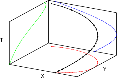
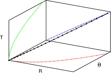
Figure 2: Representation of component trajectory. In the left panel, the thick black line with dots denotes the trajectory in the $(X,Y,T)$ 3-dimensional coordinate system, while the thin red, blue and green lines with dots denote the trajectories in the $(X,Y)$, $(X,T)$ and $(Y,T)$ projected planes; in the right panel, the thick black line with dots denotes the trajectory in the $(R,\theta,T)$ 3-dimensional coordinate system, while the thin red, blue and green lines with dots denote the trajectories in the $(R,\theta)$, $(R,T)$ and $(\theta,T)$ projected planes.

3 The regression strip algorithm

To minimize the confusion, increasing the sampling and data quality is desirable, meanwhile one should resort to an objective method to figure out the component correspondence at different epochs. To this end, we have developed an algorithm to iteratively find the most significant patterns in multi-epoch data, determine component matching and fit the trajectories over time. Like the ‘clean’ deconvolution method which gradually reaps signal from a residual image, our method progressively strips out tangled components from a trajectory pattern. By analogy, we call it ‘regression strip’ method.

The strip algorithm consists of two cycles: a major cycle for pattern recognition and a minor cycle for regression analysis. The flowchart of the algorithm is given in Fig. 3.

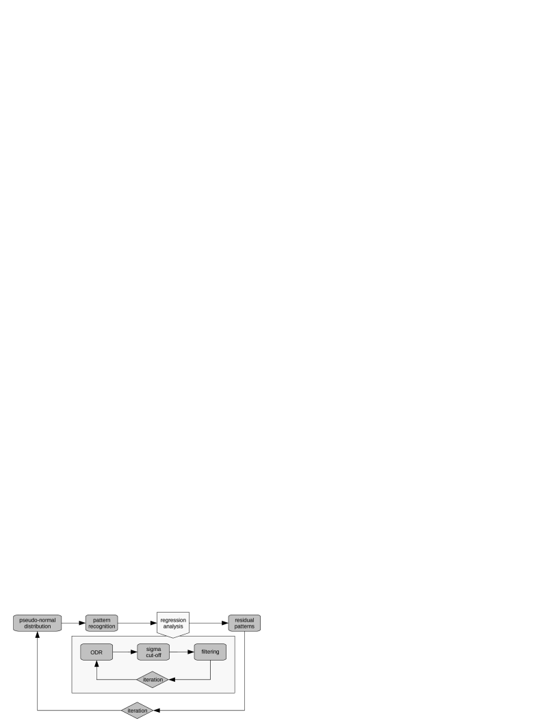
Figure 3: The flowchart of the regression strip algorithm. The inner light-shaded region encompasses the regression analysis accomplished in the minor cycle, while the unshaded outer region represents pattern stripping during the major cycle.

• The major cycle proceeds as follows:

  (i) Calculate the pseudo-normal distribution of the sampled component positions. Assuming there are intrinsic linear or non-linear patterns in those positions and the patterns for different components are similar, we can determine an overall direction where the pattern flows. We call it the pseudo-tangential direction and its orthogonal direction the pseudo-normal direction, as represented in Fig. 4. For linear patterns, this is a trivial transformation between orthogonal coordinates. For non-linear patterns, pseudo-tangential and pseudo-normal directions may always be found locally, while an overall adjustment may be made in a second stage.

  (ii) Search for significant patterns in the sampled component positions. If there are distinguishable patterns in those positions, the pattern probability distribution will show maxima in the pseudo-normal direction with appropriate binning.The sampled data corresponding to those maxima are then drawn and used as input for the subsequent regression analysis, representing initial local patterns.

  (iii) Carry out regression analyses on the data drawn in step (ii). We can do either linear or non-linear curve fitting. Note that the patterns identified at this stage are used only as a starting point for the major cycle. The data are then re-striped in the minor cycle until the regression process is stabilized.

  (iv) Remove the fitted components and get residuals. We assume that the regression process can find and fit all components, and that the remaining components can be extracted by accomplishing further iterations.

  (v) Check results against the iteration condition, if satisfied then go to step (i). The iteration condition may be either an iteration number or a physical parameter like the residual sample size.

• The minor cycle proceeds as follows:

  (i) Fit regression curves to the patterns identified during the major cycle by minimising orthogonal distances. This fitting is accomplished with the odrpack subroutines (Boggs et al., 1989).

  (ii) Cut off data points that show departures above a certain sigma level. This process not only excludes data belonging to adjacent patterns, but also reintroduces those not part of the patterns considered in previous iterations. The cut-off level is regulated by a loop gain, which is scaled down at every iteration. This limits the exclusion of good points as the iteration process converges.

  (iii) Filter the components according to their strength or post-fit deviations to make sure resolved components are assigned to different patterns. As this stage, component correspondence is also sorted out.

  (iv) Check results against the iteration condition, go to step (i) if required. A similar criterion as that in the major cycle is used to assess convergence.

In the minor cycle, component trajectories are tuned at each iteration while the deviations are reduced, and the linear or non-linear shapes are adjusted gradually. This resembles a serial squeeze-‘n’-tweak effect, as shown in Fig. 4.

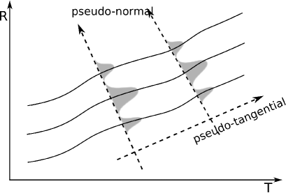
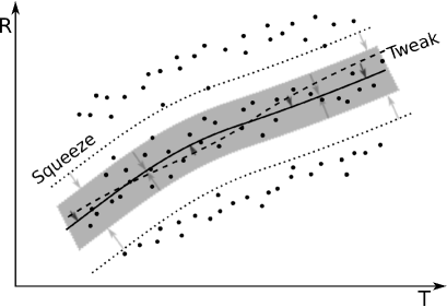
Figure 4: Pseudo-normal distributions and regression strip algorithm. The left panel shows the pseudo-tangential and pseudo-normal directions. The pseudo-normal direction is locally orthogonal to the pseudo-tangential direction where the pattern flows. The right panel shows the squeeze-‘n’-tweak effect of the regression strip algorithm.

Our sand pipeline only needs sources to be extracted in the image-plane for the initial input. Component parameters derived in further stages are obtained from model fitting both in the image-plane and the $uv$-plane. This is useful for cross-checking and to eliminate spurious components. The regression strip algorithm does not require frequent nor even sampling. The basic principles that make the method work are: (i) component trajectories show distinguishable linear or non-linear patterns, as reflected by peaks above a certain significance level in the pattern probability distribution along the pseudo-normal direction; (ii) the stripping algorithm in the regression analysis is progressive, with the squeeze-‘n’-tweak process not degrading statistical properties of the pseudo-normal distribution; (iii) deviations are reduced at every iteration, ensuring convergence of the algorithm.

4 Mock data tests

Our regression analysis does not involve cubic or higher-order non-linear fitting because the sand pipeline serves as an initial astrometric sifter and quadratic fitting can handle curved trajectories competently in most cases. In Section 4.4 below, we demonstrate that more complex trajectories can be treated locally as a set of superposed scaled quadratic curves. If the trajectory bends significantly, there should be also a notable rotating pattern in the position angle (PA) coordinates. Such peculiar sources must be investigated on a case by case basis. Furthermore, if one really wants to try the regression strip algorithm on highly non-linear data, one way to proceed is to strip the trajectory pattern section by section. In this case, one needs to make sure that the binning provides sampling along the pseudo-tangential direction that is dense enough in every individual section. In order to demonstrate the ability of the sand pipeline to resolve component trajectories, we have generated mock data which we have subsequently analysed with sand. The results derived for some typical cases are discussed below.

4.1 Affine transformation for linear patterns

If component trajectories are linear, we can demonstrate that there is an affine transformation between the pseudo-normal coordinates and the trajectory coordinates, which only involves rotation, translation and scaling. When patterns are well separated, as in the three-component test case in Fig. 5, linear trajectories are easily identified through the regression strip process. When transformed into the pseudo-normal dimension, those linear trajectory patterns correspond to distinct pseudo-normal distributions (see left panel in Fig 5). The issue of finding component trajectories then becomes equivalent to searching significant distributions in the pseudo-normal dimension.

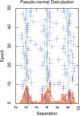
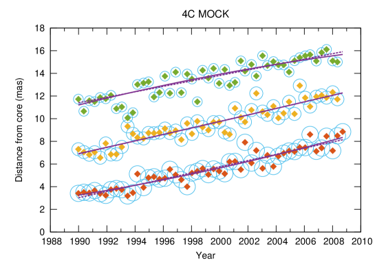
Figure 5: Pseudo-normal distributions and regression strip results with linear mock data. The left panel shows the generated mock data in the pseudo-normal dimension. The histograms and the superposed multiple Gaussian fits illustrate the significance of these pseudo-normal distributions. The right panel illustrates the capability of the regression strip algorithm to disentangle linear proper motions from series of component positions. The purple dashed lines indicate linear fits while purple solid lines indicate quadratic fits. All components are shown as light-blue circles with a size corresponding to the order of extraction, which is flux related. They are also plotted as coloured diamonds inside those circles, each colour denoting a different pattern (red, yellow and green sequentially).

4.2 The squeeze-‘n’-tweak process for non-linear patterns

If component trajectories are non-linear, mathematically there is no such affine transformation to directly convert trajectory coordinates to pseudo-normal coordinates. However, due to the built-in self-adapting capability of the regression strip algorithm, the squeeze-‘n’-tweak process is still able to disentangle component trajectories properly, provided that non-linearity remains moderate.

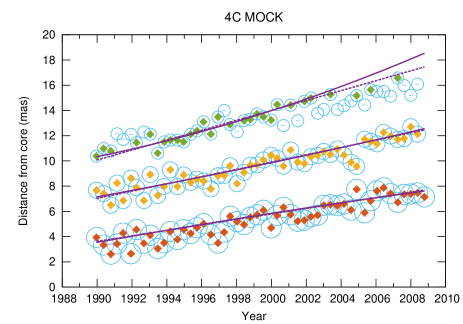
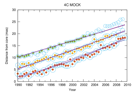
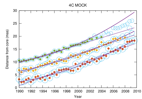
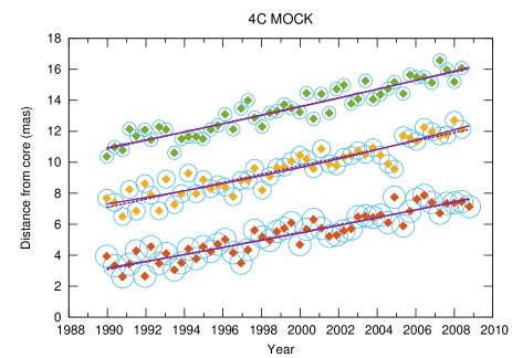
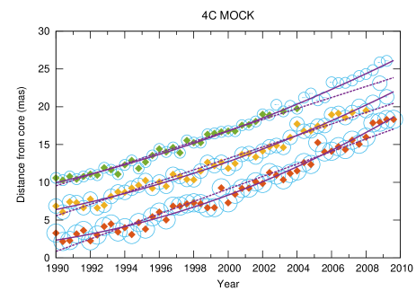
Figure 6: Illustration of the squeeze-‘n’-tweak effect with mock data. Panels on the left-hand side are for linear data while those on the right-hand side are for non-linear data. Each panel provides results at a different stage of the iterative process within the minor cycle. From the upper to lower panels, the iteration numbers are: 1, 2, and 3 for the linear data (left panels), and 1, 3 and 5 for the non-linear data (right panels), respectively. Both linear and quadratic fits are plotted in every panel for comparison purposes. Symbols are the same as those in Fig. 5. The dashed lines inside the blue circles show the diminished error bars of the mock data.

As shown in the left-hand side panels of Fig. 6, for linear patterns with small dispersion, the component trajectories are already fitted pretty well after the first iteration, except that in this case the third component is not picked up at all epochs. This is because the regression strip algorithm first picks up components in the bin with the highest counts and the resulting deviations from linear fitting remain small due to the limited sampling. In subsequent iterations, further components are introduced and the initial tight sigma cut-off is progressively released. The points scattered from the trajectory are then gradually recovered and optimal fits are obtained at the end of the iterative process.

In the case of non-linear patterns, it is more difficult to obtain a reasonable fit after the first iteration if trajectories shows significant bending, as shown in the right-hand side panels of Fig. 6. This is because there is no static pseudo-tangential direction valid for all data points. However, we still find that the squeeze-‘n’-tweak process gradually adjusts the quadratic curves in subsequent iterations to pass through the trajectory patterns, with convergence obtained after only a few iterations within the minor cycle.

We intentionally kept both linear and quadratic fits in Fig. 6 for comparison. As expected, the results of these are nearly identical for linear trajectories, whereas quadratic fits are found to reproduce more closely the tail ends of the observed patterns for non-linear trajectories.

4.3 Effects of binning and cut-off level

Most of the examples shown above have visually discernible trajectory patterns. Additional investigations on how the regression strip method works for less discernible trajectory patterns and assessment of its limits in those cases remains of interest for a wider use of the algorithm.

Considering that a distribution is always scalable, we may introduce a dimensionless quantity, the degree of separation of two normal distributions, to investigate such cases. This quantity is defined as:

$$DS:=\frac{\Delta\mu}{\sigma_{\rm max}},$$ (1)

where $\Delta\mu$ is the separation between the means and $\sigma_{\rm max}$ is the larger of the standard deviations of the two distributions. A large $DS$ value indicates that the two adjacent populations of points are well-separated, which implies a higher statistical significance for the pseudo-normal distributions. For example, the $DS$ value for the mock data in Fig. 5 is equal to 6.6, which should be viewed as a ‘well-resolved’ case.

The implementation of the regression strip algorithm in the sand pipeline incorporates parameters to control the number of bins, the sigma cut-off, the number of iterations and the loop gain. The number of iterations and loop gain mainly control the convergence speed of the regression strip process. On the other hand, the number of bins and sigma cut-off play important roles in trajectory pattern recognition. It appears that the statistics involved in such recognition are indeed very sensitive to how the data are binned when the sampling size is limited, especially where neighbouring trajectory patterns start to amalgamate.

It is worth pointing out that the PA information has not been considered in our mock data tests since our intent was to characterize proper motions in trajectory coordinates. However, the sand pipeline can deal with patterns in both trajectory and PA coordinates at the same time. Normally, a linear proper motion pattern in trajectory coordinates corresponds to a collimated pattern in PA coordinates. In the regression strip process, a sigma cut-off on both distance and PA deviations may hence be considered. In order to assess the pattern recognition limits of the algorithm, several challenging cases are considered in the sub-sections below.

4.3.1 Linear patterns with small $DS$

For ‘well-resolved’ trajectory patterns, it is found that linear patterns can be extracted correctly if the number of bins is set to a couple of tens and the cut-off level is set to a couple of sigmas. However, for smaller $DS$ values (see below), the data points gradually tangle in trajectory coordinates, which requires fine tuning on the number of bins and sigma cut-off.

The two panels in the left-hand side of Fig. 7 show results of the strip algorithm in a case where $DS=4$. When the data are gridded with 10 bins and the cut-off level is set to 6$\sigma$ (upper panel), one sees that the algorithm is not able to properly disentangle the trajectory patterns and leads to implausible results. This is because a small number of bins and a large sigma cut-off encompass too many points from adjacent patterns when neighbouring trajectory patterns are entangled, a situation that confuses the fit. Additionally, the data points left out from stripping can further degrade the situation in subsequent iterations. On the other hand, when the number of bins is increased to 20 and the cut-off level is reduced to 3$\sigma$ (lower panel), the fit becomes more reasonable. The trade-off, however, is that some data points remain left out from the fitted trajectories due to a smaller tolerance in the data selection.

The two panels in the right-hand side of Fig. 7 provide results for a test case where $DS=3.1$. Visually, it is already difficult to discern any obvious pattern if plotting all data with the same symbol. Clearly, the increased scatter in the sampled data (as implied by the smaller $DS$ value) is causing confusion in the recognition of adjacent patterns. As before, with 10 bins and a 6$\sigma$ cut-off level (upper panel), the fitted trajectories make no much sense. When increasing the number of bins to 30 (lower panel), the situation improves and reasonable results are then derived. This shows that one is less likely to get confusion at early stripping stages if starting from a smaller bin width. Evidently, the use of such a reduced width should not compromise the data sampling.

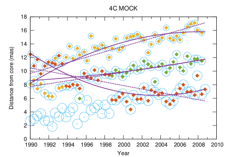
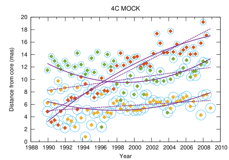
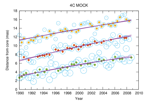
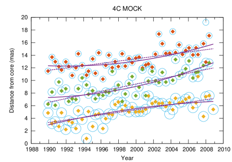
Figure 7: Effects of binning and cut-off level on linear mock data. Panels on the left-hand side are for a $DS$ value of 4, while [rgb]1.00,0.00,0.00those on the right-hand side are for a $DS$ value of 3.1. The number of bins and sigma cut-off are (10, 6) and (20, 3) for the upper and lower left-hand side panels, and (10, 6) and (30, 6) for the upper and lower right-hand side panels, respectively. Symbols are the same as those in Fig. 5.

4.3.2 Non-linear patterns with small $DS$

Because non-linear trajectory patterns do not flow in a straight pseudo-tangential direction, increasing the number of bins will degrade statistics at some point. Though a larger sigma cut-off could compensate the effect to some extent, it may also compromise the fits since a higher fraction of data from adjacent patterns are then also likely to be picked up, hence adding further confusion in the pattern recognition.

The three panels in the left column of Fig. 8 show results of such non-linear fits for $DS=4$. Going from the upper panel to the middle panel, the sigma cut-off level is increased from 3 to 6 while keeping the number of bins equal to 10. As noticeable when comparing the plots in the two panels, a notable effect of this change is that a number of data points previously left out are recovered. When the number of bins is increased to 20 (lower panel), confusion appears to be reduced, but the data points picked-up for the linear fit during initial stripping are also thinned out.

The panels in the right column of Fig. 8 show similar tests but with a value of $DS$ reduced to 3.1, i.e. in a case with more entangled trajectory patterns. Since quadratic patterns are more capable to bend the direction of the flow than linear patterns do, the data points initially picked-up for the squeeze-‘n’-tweak process need to be carefully inspected , otherwise the fitted quadratic patterns can go astray. Comparing results in the upper and middle panels, which were derived with 10 bins but with a cut-off level at 3-$\sigma$ and 6-$\sigma$, respectively, one can see that the fitted trajectories mostly differ towards their tail ends. This is because setting a certain sigma cut-off can either include or exclude some pivotal points which affect the curvature of the fitted patterns. Decelerating patterns may always be rejected since our mock patterns were set to accelerate. An increase of the number of bins from 10 to 15, as in the case reported in the lower right panel of Fig. 8, allows one to recover the curved trajectory of the third component.

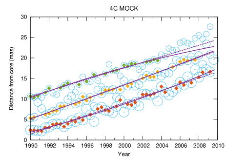
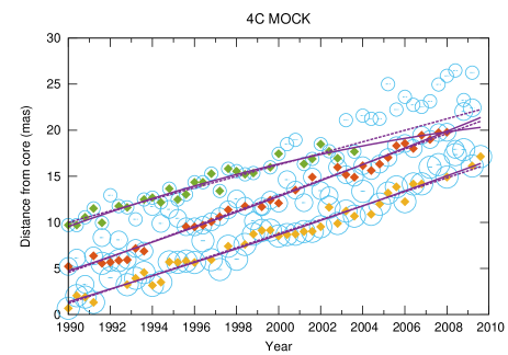
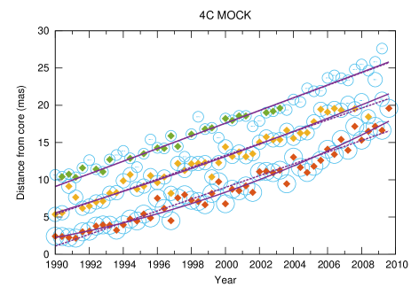
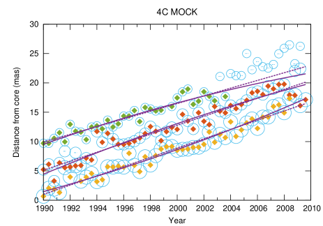
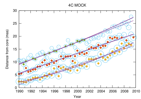
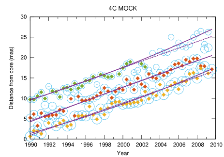
Figure 8: Effect of binning and cut-off level on non-linear mock data. Panels on the left-hand side are for a $DS$ value of 4, while those on the right-hand side are for a $DS$ value of 3.1. The number of bins and sigma cut-off are (10, 3), (10, 6) and (20, 6) for the upper, middle and lower left-hand side panels, and (10, 3), (10, 6) and (15, 6) for the upper, middle and lower right-hand side panels, respectively. Symbols are the same as those in Fig. 5.

4.3.3 Extreme cases with $DS<3$

Results for a non-linear case with $DS=2.6$ are reported in Fig. 9. Comparing with the known patterns of the mock data indicates that the regression strip algorithm cannot properly disentangle the trajectory patterns in such a case no matter how the number of bins and sigma cut-off are tuned. Some results may look plausible but they either miss out many data points or produce wrong accelerations.

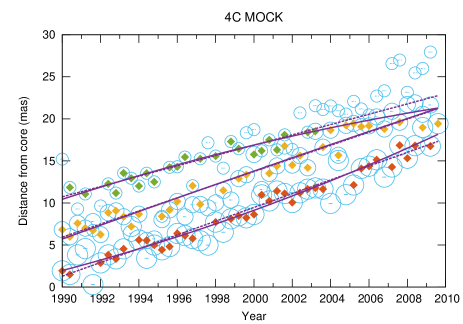
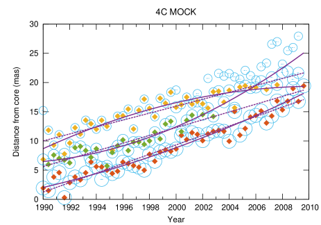
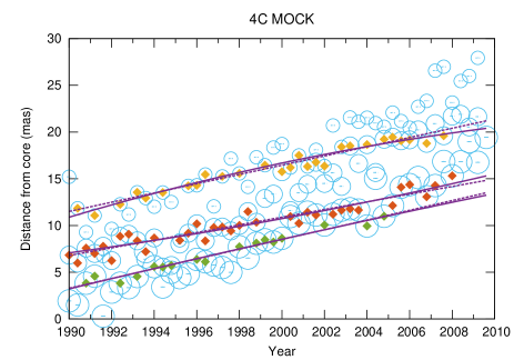
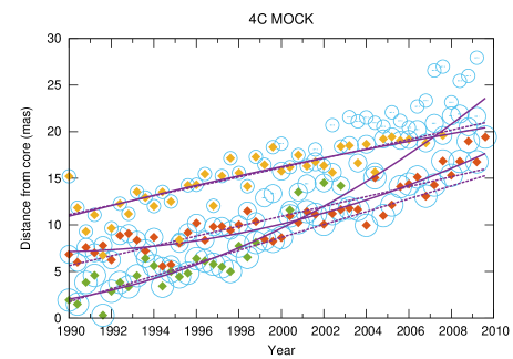
Figure 9: Effects of binning and cut-off level on non-linear mock data with $DS=2.6$. From left to right and for the upper to lower panels, the number of bins and sigma cut-off are (10, 3), (10, 6), (15, 3) and (15, 6), respectively. Symbols are the same as those in Fig. 5.

From the examples above, we find that the regression strip algorithm can resolve trajectory patterns easily when the $DS$ value is larger than 3. However, when the $DS$ value is smaller than 3, the algorithm approaches its limit. This is analogous to the situation for a Gaussian beam where two convolved point sources need to be at least one beam width apart (fwhm $\simeq 2.4\sigma$) to be resolved. Based on the statistics for our pseudo-normal distribution, it appears that the threshold for $DS$ should be even raised further due to the discrete and limited sampling of the data sets.

4.4 DS-curvature degeneracy

For non-linear quadratic trajectories, we find that there is a degeneracy between $DS$ and the local curvature. The local curvature of a univariate quadratic function expressed in the form of $y(x)=ax^{2}+bx+c$ is given by

$$k=\frac{y^{\prime\prime}}{(1+y^{\prime 2})^{3/2}}=\frac{2a}{[1+(2ax+b)^{2}]^{3/2}}\leq 2a.$$ (2)

At the extreme curvature points, $k_{\rm max}=2a$ which is a constant. For different sets of quadratic trajectories, the local pattern configurations only differ by a scaling factor, as illustrated by tests using our regression strip algorithm.

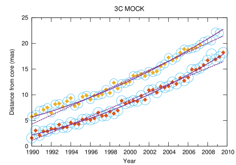
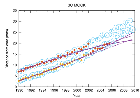
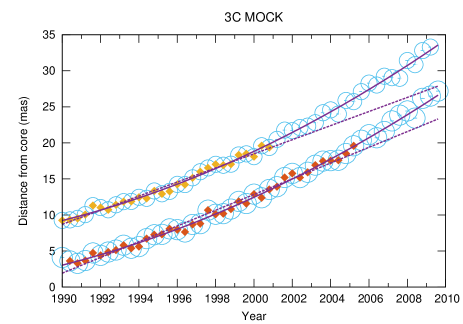
Figure 10: The DS-curvature degeneracy in the case of quadratic trajectories. In these plots, the $DS$ and $k_{\rm max}$ values are (8, 0.02), (8, 0.03) and (12, 0.03) for the upper, middle and lower panels, respectively. Symbols are the same as those in Fig. 5.

The plots in Fig. 10 show that for two well stripped trajectory patterns, the regression strip algorithm gets confused if the curvature is scaled to one and a half times the original value. However, the confusion goes away if the $DS$ value is also scaled by the same amount. If noting $DS_{n}$ the component of $DS$ in the pseudo-normal direction and $DS_{y}$ the scaled value of $DS$ in the Y direction (see Fig. 11), it can be proved that

$$DS_{n}\leq DS_{y}\cdot\cos\theta,\quad\textrm{and}\quad x\uparrow\;\theta\downarrow\;DS_{n}\uparrow\;DS_{y}\uparrow.$$

In this case, the trajectory patterns are so well separated near their tail ends where $x\gg 1$ that the algorithm has no problem picking them up even with a larger sigma cut-off.

Figure 11: Illustration of the $DS$ variation for non-intersecting quadratic curves. $DS_{n}$ is the component of $DS$ in the pseudo-normal direction, $DS_{y}$ is the scaling of $DS$ in the Y direction, and $\theta$ is the angle between $DS_{n}$ and $DS_{y}$.

5 Trials with real observations

5.1 Description of data

VLBI observations are generally categorized into two broad classes, those dedicated to geodesy and astrometry and those dedicated to astrophysics. They are both based on the same technique but have different scopes. Astrometric VLBI is targeted to finding compact and stable sources over the entire sky to construct highly-accurate celestial reference frames, while astrophysical VLBI is more focused on extended and variable sources which are best to study internal physical processes in the sources. Since the radio source count drops with frequency, astrometric VLBI has mostly concentrated on observing at centimetre wavelengths. On the other hand, astrophysical VLBI may be conducted up to millimetre wavelengths for higher resolution. Nevertheless, there are a number of common sources between these programmes since all-sky surveys have been conducted on each side. In this light, our pipeline is of high interest since it can efficiently cross-examine multi-epoch multi-band VLBI data from various programmes for better modelling.

For demonstrating the capabilities of our pipeline, we have tested it on data from several VLBI monitoring programmes, available either publicly or through our collaboration. These include the RDV, MOJAVE and VLBA-BU-Blazar programmes. The RDV observations have a primary geodetic-astrometric scope, while the MOJAVE and VLBA-BU-Blazar observations have astrophysical scopes.

5.2 The source of interest: 1308+326

The radio source 1308+326 is a well-known quasi-stellar object (QSO) that has been a target of the RDV, MOJAVE and VLBA-BU-Blazar monitoring programmes. VLBI images of 1308+326 (see Fig. 17) reveal that its morphology became more complex and more extended starting from around 2000. For this reason, the RDV observations were strongly reduced afterwards and there is only sparse data beyond 2004. On the other hand, the MOJAVE data of 1308+326 span over two decades (since 1995). The more recent VLBA-BU-Blazar observations were initiated in 2009. In this paper, we use 1308+326 only for demonstration purposes, rather than for a thorough study of the kinematics of its jet.

5.3 Detection of proper motions

As shown above, trajectory pattern recognition takes place at the same time as the regression analysis in the regression strip algorithm implemented in the sand pipeline. When a trajectory pattern is identified, proper motions are thus determined concurrently. Such proper motions may be further used to study jet kinematics and constrain active galactic nucleus (AGN) models. Tests using mock data have shown that the algorithm can cope with a variety of situations. In reality, one has to bear in mind that the results of the fits depend at some level on the data sampling, hence a favourable situation may deteriorate if the data sampling is inadequate. In the following, we discuss the proper motions determined with our algorithm at the S band, X band, K band and Q band frequencies.

At the S band frequency, the detected proper motion pattern is significant and one sees that it can be characterized simply with a single component (Fig. 12). This is because the resolution at S band is lower. While a straight line fits the proper motion of this unique component fairly well, a number of outliers are found around epoch 2003. Such a scatter may be caused by a newly-born component emerging from the core by that time. However, no firm conclusion can be drawn in the absence of regular observations beyond 2004. From the PA plots in Fig. 12 (right panels), it is found that the detected jet component roughly moves along a straight line, though with a slight turning over time. Comparing the fits in the image plane (upper panels) and $uv$-plane (lower panels) shows that the results derived with the two approaches are consistent within half a milliarcsecond. A linear fit of the component proper motion then leads to an angular speed of 0.358$\pm$0.015 mas yr^-1. In a final stage, our pipeline automatically checks the NED database to retrieve the source redshift and derive its angular diameter distance with an embedded cosmological calculator. At a redshift of 0.996, the angular proper motion for 1308+326 corresponds to an apparent superluminal velocity of 18.1 c.

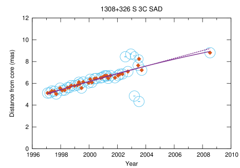
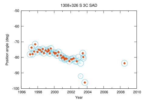
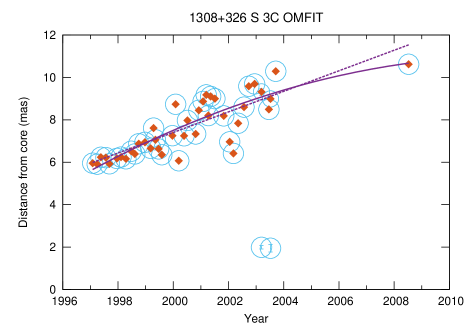
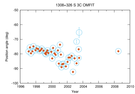
Figure 12: Proper motion patterns for 1308+326 at the S band frequency, as inferred from model-fitting in the image-plane (upper panels) and $uv$-plane (lower panels). The left panels show distances to the core while the right panels show radial position angles. Symbols are the same as those in Fig. 5.

At the X band frequency, two significant proper motion patterns are identified, both of which can be easily fitted with a straight line or a quadratic line (Fig. 13). The $DS$ value for these patterns is about 3.8. In Fig. 13, the different colours assigned to components in the same pattern indicate that all such components were not extracted at the same iteration. The components are mostly ordered according to their flux when extracted, but this does not correspond to reality because component brightness varies with time. The correct component assignment is determined when the fit is tuned during the squeeze-‘n’-tweak process. Just as at the S band frequency, components belonging to the same pattern roughly line up but the direction of motion is changing with time (see plots in the right panels of Fig. 13). The scatter around 2003, when a new component is suspected to emerge, is found at X band too. The fitted angular speeds of the two detected components are 0.351$\pm$0.015 mas yr^-1and 0.376$\pm$0.018 mas yr^-1, corresponding to apparent superluminal velocities of 17.8 c and 19.0 c, respectively.

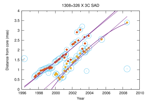
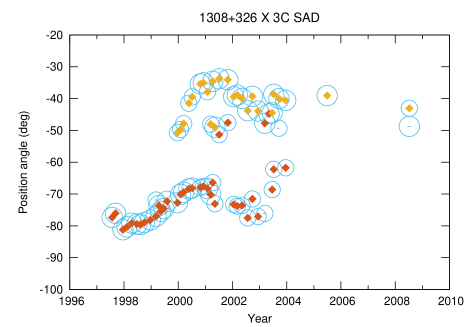
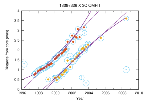
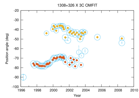
Figure 13: Proper motion patterns for 1308+326 at the X band frequency, as inferred from model-fitting in the image-plane (upper panels) and $uv$-plane (lower panels). The left panels show distances to the core while the right panels show radial position angles. Symbols are the same as those in Fig. 5.

Based on the series of images generated by the sand pipeline, 1308+326 was found to have more complex structure at higher frequencies, namely K band and Q band. This is not only because the extended radio emission is resolved into discrete components at these higher frequencies, as a result of higher resolving power, but also because the higher-frequency images reveal intense kinematics of the jet close to the AGN core. The complexity of the brightness distribution is also reflected in the difficulty of proper motion pattern recognition, as shown in Fig. 14. To illustrate how observing frequency affects such recognition, we have conservatively set the control parameters for our tests. Although the MOJAVE data cover a longer time span, the sampling of these data is neither frequent nor even. As a result, regression stripping stopped after fitting three proper motion patterns, with the residual data points not having enough significance for further fitting. The $DS$ value of the first two fitted patterns is about 2.4. Of course, we could visually fit at least two additional patterns but these would not be reliable because of the lack of data points. Furthermore, we see from the plots in Fig. 14 that our pipeline even tried to do a quadratic fit for the third proper motion pattern when model-fitting the data in the image plane. Since the residual data points from epoch 2012 could belong to the emerging fourth component and such an erratic behaviour is not verified with $uv$-plane fitting, it appears difficult to trust those fits. In practice, we can simply restrain the initial statistical criteria and let the regression strip algorithm exclude such situations.

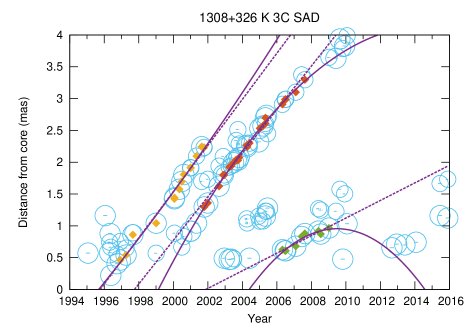
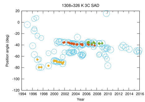
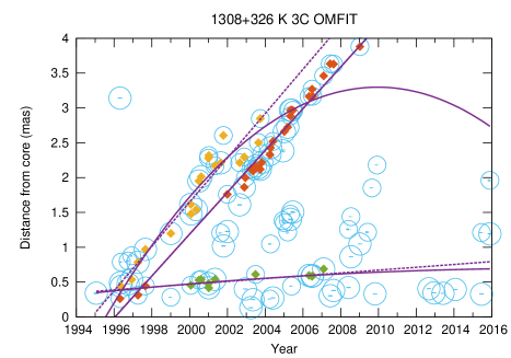
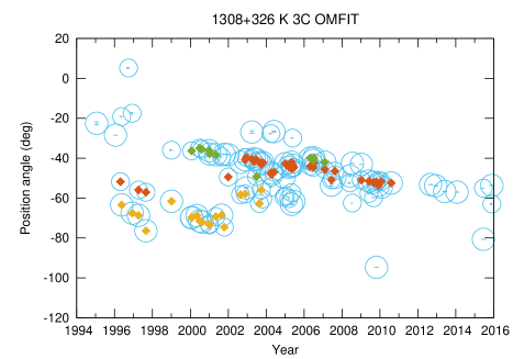
Figure 14: Proper motion patterns for 1308+326 at the K band frequency, as inferred from model-fitting in the image-plane (upper panels) and $uv$-plane (lower panels). The left panels show distances to the core while the right panels show radial position angles. Symbols are the same as those in Fig. 5.

The Q-band proper motion patterns do not look optimal either, because the data points are even more scattered, as seen from Fig. 15. The $DS$ value of the first two significant patterns is about 1.6, hence likely to lead to confusion as illustrated in Fig. 1. Generally source expansion is favoured over source contraction, which provides further constraints. However, contradictory measurements of superluminal motions when determined by different groups are not unlikely due to such confusion (Piner & Kingham, 1997).

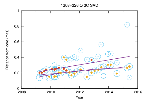
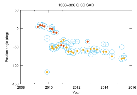
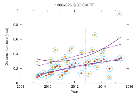
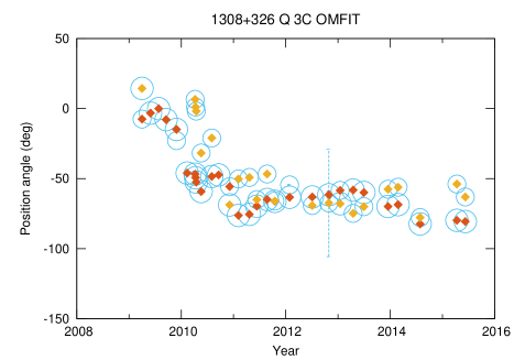
Figure 15: Proper motion patterns for 1308+326 at the Q band frequency, as inferred from model-fitting in the image-plane (upper panels) and $uv$-plane (lower panels). The left panels show distances to the core while the right panels show radial position angles. Symbols are the same as those in Fig. 5.

One potential issue to be pointed out is the registration error in the alignment of the core component for multi-epoch data. Due to the regular emergence of jet components, the centroid of the core may shift with time, hence causing errors in the relative positions of the outer jet components at different epochs. Such offsets may be inferred from the aligned and subtracted multi-epoch images, within the detection limit of the interferometer, and should be corrected for the highest accuracy when calculating relative component positions.

6 Conclusions

The comprehensive VLBI data reduction pipeline sand is designed to help radio astronomers to improve the efficiency and objectivity of interferometric data reduction. For multi-epoch multiband observations, the pipeline provides a complete initial set of source parameters, derived from imaging and model fitting, which may be systematically analysed in spatial, temporal and spectral domains at the post-processing stage. It also offers a means to combine and analyse heterogeneous data sets from different resources consistently. With various VLBI observing programmes going on, this aspect is of high interest and may be viewed as an analogue to what Virtual Observatory projects pursue.

The sand pipeline has a built-in regression strip algorithm which automatically identifies jet component trajectories and fits proper motions at the same time (see Sect. 3). The algorithm was found to work well when trajectory patterns between components are well separated.

The pipeline is not a fully-competent artificial-intelligence substitution to manual VLBI data reduction. However, it provides an objective approach to cross-examine results from different research groups. When used for massive data reduction, it also offers a practical tool to sift out peculiar sources of interest for extended studies.

Acknowledgements

MZ is grateful to the Centre National de la Recherche Scientifique (CNRS) for granting a post-doctoral fellowship at the Laboratoire d’Astrophysique de Bordeaux (LAB) in France to develop the pipeline infrastructure reported in this paper. This work was further supported by the National Basic Research Programme of China (2012CB821804 and 2015CB857100), the National Science Foundation of China (11103055) and the West Light Foundation of Chinese Academy of Sciences (RCPY201105). This research has made use of the NASA/IPAC Extragalactic Database (NED), which is operated by the Jet Propulsion Laboratory, California Institute of Technology, under contract with the National Aeronautics and Space Administration (NASA). This research has also made use of data from the MOJAVE database which is maintained by the MOJAVE team (Lister et al., 2009), and from the VLBA-BU-Blazar Monitoring Program at 43 GHz which is funded by NASA through the Fermi Guest Investigator Program (Marscher et al., 2009). The VLBA is an instrument of the National Radio Astronomy Observatory, a facility of the National Science Foundation operated by Associated Universities, Inc. The authors also thank the Open Source software packages Scipy (Jones et al., 2001), Gnuplot (Williams et al., 04) and Gnuplot-py (Haggerty, 03), which made the development of this pipeline easily achievable and transferable.

Appendix A The SAND pipeline scheme

A major advantage of the sand pipeline is that it can benefit from the robustness of well-tested aips tasks and of the computational functionality of the Python language to develop various user-customized data reduction algorithms. The pipeline is composed of structured modules, which facilitates incorporation of initial calibration and self-calibration procedures, provided that flagging and calibration tables are available in machine-readable form. This is generally the case for VLBI post-correlation processing pipelines, e.g. those implemented at the European VLBI Network (EVN) or Very Long Baseline Array (VLBA) facilities. Additionally, many databases provide $uv$ data that are already calibrated. For this reason, we focus on the imaging and model-fitting procedures behind sand in the following sections.

A.1 Categorizing the data

As a general approach, our pipeline has not been designed to deal with any specific observing programme. It thus has the capability to handle data from various archives which often have different conventions for naming and ordering sources. The sand pipeline converts between B1950 and J2000 source names and indexes every data file in a unique way based on metadata information (source name, observing band, session number, …). Heterogeneous data sets are thus easily imported, and targeted reductions on a certain observing band or session range, for any particular list of sources, may be accomplished. All results from processing are stored in specific repositories with unique identification, allowing multiple pipeline processes to be run concurrently without confusion in the outputs. This scheme is especially useful to cross-check the effects of a certain parameterization or to explore various aspects of the parameter space in parallel.

A.2 Imaging

Deconvolution of the $uv$ data is accomplished using the Clark (1980) clean algorithm with the Schwab & Cotton (1983) scheme for subtraction in the $uv$-plane, as implemented in the aips task imagr. Component search and extraction from the cleaned image is conducted with the task sad which looks through the image plane to find bright peaks above a certain flux threshold and simultaneously fits those with elliptical Gaussians. The image quality is closely tied to the $uv$ coverage and depends on the deconvolution algorithm. Gaps in the $uv$ sampling introduce gridding errors which affect the synthetic beam and cause non-Gaussian residuals during the deconvolution process which are difficult to eliminate. Conversely, Gaussian noise spikes may be more easily rejected since the corresponding flux is usually smeared out below the given flux threshold.

A.3 Model fitting

The on-the-fly model-fitting using the task sad is generally good enough for discrete compact sources. For more complex cases, we have implemented an extra module based on the specific image-plane model-fitting task jmfit, permitting further verification of the model parameters. Additionally, we check component separation against the beam size. If separation is less than half a beam size, the corresponding component is tagged as confused. Such confused components are either treated as a single component in a subsequent processing stage or “forced” to have a more significant separation by constructing a super-resolved map with a smaller beam size.

A.3.1 Image-plane fitting

Component extraction in the image plane with task sad is based on the Gaussian fitting subroutine behind task jmfit. We have demonstrated that in most cases the models derived from the two tasks are identical. However, the task jmfit offers a wider range of options for parameter settings, which is of interest for sources with subtle structures requiring specific attention. Such sources generally show extended structures and low-brightness features, requiring appropriate setting of the window size to get optimum results.

A.3.2 $uv$-plane fitting

As an ill-posed inverse problem, a deconvolution has no unique solution. The main goal of deconvolution algorithms then is to achieve an optimal convergence. The clean algorithm works well in many cases, especially when source structure is compact. However, compact radio sources may also show extended features, in particular at low frequencies. Due to the ‘clean bias’ (Condon et al., 1998), a cleaned image might not preserve authentic structures, notably when the source is extended or weak. Nevertheless, the uncertainties introduced by the clean algorithm should be largely reduced if fitting models directly in the $uv$ plane.

Model-fitting in the $uv$ plane requires the input structural model of the source to be well defined beforehand (e.g. in the form of a single elliptical Gaussian) to be Fourier-transformed into the $uv$ plane. Having a proper input model is important in this process as model-fitting in the $uv$ plane does not always converge, in particular when the actual source structure departs significantly from the model fed as input or if the source is too weak. It is to be noted that the task omfit used to perform model-fitting in the $uv$-plane has the same self-calibration capability as difmap during cleaning, hence providing consistent schemes. The results from modelling in the image-plane may thus be used to provide the required input for modelling in the $uv$-plane.

A.3.3 Comparison with manual reduction

To assess the quality of the models determined by sand, we have compared our pipeline results with those derived from a manual reduction of the RDV data by Piner et al. (2012). Due to the degeneracy between elliptical and circular Gaussians, and to avoid confusion, we have restricted the shape of our component models in the $uv$-plane to circular Gaussians. A detailed comparison of the results from sand and from Piner et al. (2012) for the core and the first two jet components for 1308+326 is shown in Fig. 16. The comparison indicates that the fitted parameters are quite consistent for the two determinations. The only noticeable discrepancies are in the position angles of the elliptical Gaussians, which is not unexpected since we used circular Gaussians and Piner et al. (2012) used elliptical Gaussians.

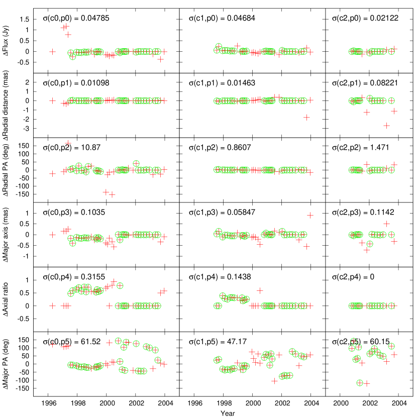
Figure 16: Differences in fitted parameters between the manual reduction of Piner et al. (2012) and the sand automatic reduction for the X-band RDV observations of 1308+326. The component sequence is denoted as {c0, c1, c2} in decreasing flux order and the parameter sequence is denoted as {p0, p1, p2, p3, p4, p5}, corresponding to the flux, radial separation, radial position angle, major axis, axial ratio and major axis position angle in accordance with the difmap conventions. The circles indicate the epochs for which the number of components in the two reductions agrees.

A.4 Generation of images and cataloguing

A.4.1 Morphological evolution

Since our pipeline has been designed to deal with multi-epoch observations we have built a module that automatically generates images at every epoch. The images are reconstructed from the fitted model parameters and are generated in parallel with the cleaned images. See Figs. 17 and 18 for an example. By inspecting such images, the evolution of jet structures can be quickly investigated and any discrepancies from the cleaned image is easily spotted. These images are also useful to identify weak features that sometimes surround major structures.

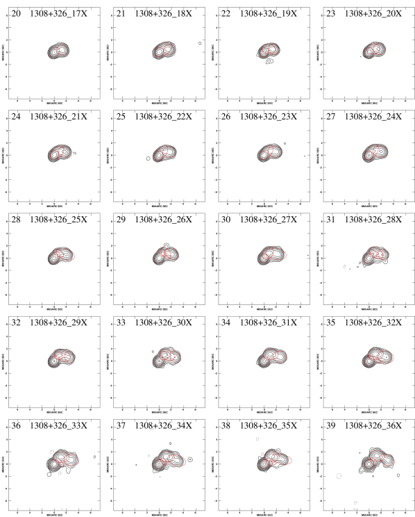
Figure 17: A sample of cleaned images of 1308+326 at the X band frequency, as derived from RDV observations with the sand pipeline. Contour levels are plotted at (-1, 1, 2, 4, 8, 16, 32, 64, 128, 256, 512, 1024) $\times\ 6\sigma$, where $\sigma$ is the off-source noise in the map. The red circles denote the modelled components. The axes are relative RA and DEC in units of milliarcsecond with the origin of the map shifted to the core centroid.

Figure 18: A sample of reconstructed models of 1308+326 at the X band frequency, as derived from RDV observations with the sand pipeline. The contour levels and units for the axes are the same as those in Fig. 17.

A.4.2 Polarization maps

If the visibility data have full correlated Stokes parameters, i.e. RR, LL, RL and LR, our pipeline will automatically consider them and produce polarization maps. As shown from the series of K-band polarization maps of 1308+326 in Fig. 19, a rotation of the polarisation angle, here in a counter-clockwise direction, is detected from the maps at the successive epochs. Based on these maps, one could also infer that the direction of the jet emission beam from the central engine slewed during this period, e.g. due to precession.

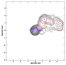
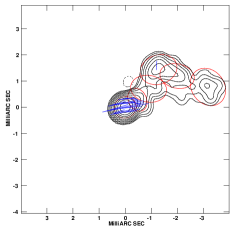
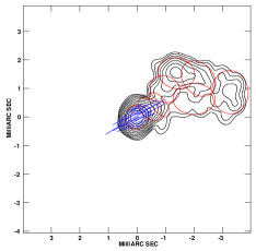
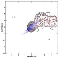
Figure 19: Illustration of the polarization angle rotation in the K-band observations of 1308+326, as determined from the sand pipeline. The contour levels and units for the axes are the same as those in Fig. 17. The red circles denote the modelled components while the blue vectors indicate the direction of the polarization emission in the core.

A.5 Post-processing

In addition to the various data reduction steps explained above, some post-processing procedures have been implemented in the sand pipeline in order to facilitate analysis and interpretation of multi-epoch multiband results. These procedures comprise the determination of component trajectories and generation of light curves and multi-epoch component spectra, as described below.

A.5.1 Component trajectories

The determination of jet component trajectories is the topic of this paper and hence is detailed in the main text. See Sect. 3 for a description of the algorithm and Sects. 4 and 5 for the results of tests with mock and real data.

A.5.2 Light curves

Following model fitting, component flux density is available at every epoch and for every band. It is thus straightforward to extract the core flux density from these and derive multi-band light curves. An example of such a light curve, as determined from sand, is shown in Fig. 20. Additionally, a capability to derive single-side Power Spectral Density (PSD) plots via direct fast Fourier transform (FFT) was implemented to check the periodicity of light curves. For simultaneous multi-band VLBI observations, even from non-coordinated programmes, the pipeline can also automatically identify and extract observations in overlapping time ranges and cross-correlate the light curves from the different bands in each range. This aspect will be discussed in details in a subsequent paper.

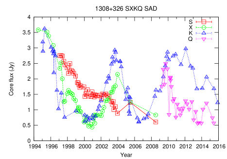
Figure 20: Multi-band variations of the core flux density in 1308+326. Symbols in red, green, blue and pink indicate flux densities at S band, X band, K band and Q band, respectively.

A.5.3 Multi-epoch spectra

Using multi-band light curves, one can also check the spectral index of the radio sources. For this purpose, a procedure that re-bins the data over the overlapping epoch ranges, calculates the average flux in each bin, and derives the source spectrum at the different epochs has been implemented in sand. An example of such multi-epoch spectra for the flat-spectrum radio source 1308+326 is shown in Fig. 21.

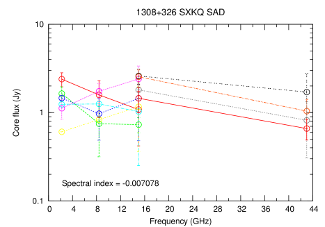
Figure 21: Multi-epoch spectra for the core component of 1308+326. Data in the same time bin are plotted with symbols of the same colour. Different colours denote different time bins. The spectral index value is determined by averaging over time.

References

- Boggs et al. (1989) Boggs P. T., Donaldson J. R., h. Byrd R., Schnabel R. B., 1989, ACM Transactions on Mathematical Software, 15, 348
- Clark (1980) Clark B. G., 1980, A&A, 89, 377
- Condon et al. (1998) Condon J. J., Cotton W. D., Greisen E. W., Yin Q. F., Perley R. A., Taylor G. B., Broderick J. J., 1998, AJ, 115, 1693
- Cotton (2008) Cotton W. D., 2008, PASP, 120, 439
- Greisen (1998) Greisen E. W., 1998, in Albrecht R., Hook R. N., Bushouse H. A., eds, Astronomical Society of the Pacific Conference Series Vol. 145, Astronomical Data Analysis Software and Systems VII. p. 204
- Haggerty (03 ) Haggerty W., 2003–, Gnuplot-py: a Python interfaces to gnuplot, http://gnuplot-py.sourceforge.net/
- Jones et al. (2001) Jones E., Oliphant T., Peterson P., et al., 2001, SciPy: Open source scientific tools for Python, http://www.scipy.org/
- Lister et al. (2009) Lister M. L., et al., 2009, AJ, 138, 1874
- Marscher et al. (2009) Marscher A. P., et al., 2009, in American Astronomical Society Meeting Abstracts #213. p. 382
- Mertens & Lobanov (2015) Mertens F., Lobanov A., 2015, A&A, 574, A67
- Piner & Kingham (1997) Piner B. G., Kingham K. A., 1997, ApJ, 485, L61
- Piner et al. (2012) Piner B. G., et al., 2012, ApJ, 758, 84
- Rossum (1993) Rossum G. V., 1993, in Proc. of the NLUUG najaarsconferentie (Dutch UNIX users group).
- Schwab & Cotton (1983) Schwab F. R., Cotton W. D., 1983, AJ, 88, 688
- Shepherd (1997) Shepherd M. C., 1997, in Hunt G., Payne H., eds, Astronomical Society of the Pacific Conference Series Vol. 125, Astronomical Data Analysis Software and Systems VI. p. 77
- Williams et al. (04 ) Williams T., Kelley C., et al., 2004–, Gnuplot 4: an interactive plotting program, http://gnuplot.sourceforge.net/
- Zhang (2016) Zhang M., 2016, SAND: Automated VLBI imaging and analyzing pipeline, Astrophysics Source Code Library (ascl:1605.015)
- Zhang et al. (2007) Zhang M., Jackson N., Porcas R. W., Browne I. W. A., 2007, MNRAS, 377, 1623