Functional equations as an important analytic method in stochastic modelling and in combinatorics

Abstract

Functional equations (FE) arise quite naturally in the analysis of stochastic systems of different kinds : queueing and telecommunication networks, random walks, enumeration of planar lattice walks, etc. Frequently, the object is to determine the probability generating function of some positive random vector in $\mathbb{Z}_{+}^{n}$. Although the situation $n=1$ is more classical, we quote an interesting non local functional equation which appeared in modelling a divide and conquer protocol for a muti-access broadcast channel. As for $n=2$, we outline the theory reducing these linear FEs to boundary value problems of Riemann-Hilbert-Carleman type, with closed form integral solutions. Typical queueing examples analyzed over the last $45$ years are sketched. Furthermore, it is also sometimes possible to determine the nature of the functions (e.g., rational, algebraic, holonomic), as illustrated in a combinatorial context, where asymptotics are briefly tackled. For general situations (e.g., big jumps, or $n\geq 3$), only prospective comments are made, because then no concrete theory exists.

AMS $2000$ Subject Classification: Primary 60G50; secondary 30F10, 30D05

1 Introduction

It is now almost undisputable that analytic methods became ubiquitous in probability. Indeed, the greek word αναλυτιϰος refers essentially to “the ability to analyze”, which is nothing else but the very nature of science ! During the last century, the impressive development of information sciences (in particular computer and telecommunications networks) led to a need of system modelling, which in turn highlighted a number of new interesting (and sometimes fascinating) mathematical objects. In the sequel, we shall focus on a particular class of these objects, namely functional equations (FE). Needless to emphasize that this subject, in the past, attracted famous mathematicians, among them d’Alembert Euler, Abel, Cauchy, Riemann…

The paper is organized as follows. Section 2 presents an interesting non local FE of one single variable, encountered in the analysis of a divide and conquer algorithm. In Section 3, we consider FE coming from the analysis of the invariant measure of random walks in the quarter plane, and show in particular how the can be reduced to Riemann-Hilbert-Carleman boundary value problems. Section 4 sketches four examples, emanating from queueing network models resolved over the last forty five-years. In a combinatorial context, Section 5 summarizes results concerning the nature of the counting generating functions, when the group of the random walk is finite. Some questions related to asymptotics are also tackled. The concluding Section 6 gives prospective remarks for more general situations (arbitrary big jumps, $n\geq 3$, etc), noting that currently no concrete global theory exists.

2 A non local functional equation of one complex variable for a collision resolution algorithm (CRA)

A huge literature has been devoted to FEs when the unknown function depends on a single variable. In this respect, the reader may see the seminal prominent book by Kuczma [16]. In a probabilistic context, we present a simple FE encountered in the analysis of a variety of the Capetanakis-Tsybakov-Mikhailov CRA, which is a divide and conquer algorithm. All proofs can be found in [7].

2.1 Specification of the CRA with continuous input

1. A single error-free channel is shared among many users which transmit messages of constant length (packets). Time is slotted and may be considered discrete. Users are synchronized with respect to the slots, and packets are transmitted at the beginning of slots only. Each slot is equal to the time required to transmit a packet (see the famous ALOHA network concept).

2. Each transmission is receivable by every user. Thus, when two or more users transmit simultaneously, packets are said to collide (interfere) and none is received correctly: these collisions are treated as transmission errors and each user must strive to retransmit its colliding packet until it is correctly received. The users all employ the same algorithm for this purpose, and have to resolve the contention without the benefit of any other source of information on other users’ activity save the common channel.

3. Each user monitoring the channel knows, by the end of the slot, if that slot produced a collision or not.

4. Each active user maintains a conceptual stack. At each slot end, he determines his position in the stack according to the following procedure (identical to all users, who are unable, however to communicate their stack state):

   • When an inactive user becomes active, it enters level $0$ in the stack. He will transmit at the nearest slot, and will always do so when at stack level $0$.

   • After a non-collision slot, a user in stack level $0$ (there can be at most one such user) becomes inactive, and all users decrease their stack level by $1$.

   • After a collision slot, all users at stack level $i,i\geq 1$ change to level $i+1$. The users at level $0$ are split into two groups; one group remains at level $0$, while the members of the other push themselves into level $1$. This partition can be made on the basis of a Bernouilli trial, each user flipping a two-sided coin (independently of the other active users) : with probability $p$, he remains at level $0$, and with probability $q=1-p$ he pushes himself into level $1$.

5. The numbers of new packets generated in each slot (i.e. the number of new active users) form a sequence of i.i.d. random variables, denoted by $X_{i},i\geq 1$, which follow a Poisson distribution with parameter $\lambda$.

The collision resolution interval (CRI), denoted in the sequal by $L_{n}$, is the time it takes to dispose of a group of $n$ colliders initially at level $0$.

2.2 Functional equation for the generating function of the mean CRI

The random variables $L_{n}$ satisfy the recursive relationship

$$\begin{cases}L_{0}=L_{1}=1,\\[5.69046pt] L_{n}=1+L_{I+X}+L_{n-I+Y},\quad n\geq 2,\end{cases}$$ (2.1)

where

• $I$, the number of messages immediately retransmitted, follows the binomial distribution $B(n,p)$;

• $X$ is the number of new arrivals in that collision slot;

• $Y$ is the number of new arrivals in the slot following $L_{I+X}$.

Moreover, $I,X,Y$ are supposed to be independent random variables

Letting $\alpha_{n}\stackrel{{\scriptstyle\mbox{\tiny def}}}{{=}}\mathbb{E}(L_{n})$ and introducing

$$\begin{cases}\displaystyle\alpha(z)\stackrel{{\scriptstyle\mbox{\tiny def}}}{{=}}\sum_{n\geq 0}\alpha_{n}\frac{z^{n}}{n!},\\[11.38092pt] \displaystyle\psi(z)\stackrel{{\scriptstyle\mbox{\tiny def}}}{{=}}e^{-z}\alpha(z),\end{cases}$$ (2.2)

we obtain the non local FE

$$\boxed{\psi(z)-\psi(\lambda+pz)-\psi(\lambda+qz)=1-2\psi(\lambda)e^{-z}(1+Kz)},$$ (2.3)

where

$$K=\frac{\exp(-\lambda p)-\exp(-\lambda q)}{\frac{\lambda}{q}\exp(-\lambda q)-\frac{\lambda}{p}\exp(-\lambda p)}.$$

From now on, $p\geq q$ with $(p+q=1)$ and $\sigma_{1}(z)\stackrel{{\scriptstyle\mbox{\tiny def}}}{{=}}\alpha+pz$, $\sigma_{2}(z)\stackrel{{\scriptstyle\mbox{\tiny def}}}{{=}}\alpha+qz$.

To solve (2.3), we need to introduce a non-commutative iteration semigroup $H$ of linear substitutions generated by $\sigma_{1},\sigma_{2}$, where the semigroup operation is the composition of functions. The identity of $H$ is denoted by $\varepsilon$, so that $\varepsilon(z)=z,\forall z\in\mathbb{C}$ (the complex plane) and any $\sigma\in H$ can be written in the form

$$\sigma=\sigma_{i_{1}}\sigma_{i_{2}}\dots\sigma_{i_{n}},\quad n\geq 0,\ i_{j}\in\{1,2\}.$$

Setting

$$|\sigma|_{1}=\mathrm{card}\{j|i_{j}=1\},\quad|\sigma|_{2}=\mathrm{card}\{j|i_{j}=2\},\quad|\sigma|=|\sigma|_{1}|+|\sigma|_{2}|,$$

we introduce the notation, valid for arbitrary complex numbers $\alpha,\beta$,

$$(\alpha;\beta)^{\sigma}=\alpha^{|\sigma|_{1}|}\beta^{|\sigma|_{2}|}.$$

By linearity, we have $\sigma(z)=\sigma(0)+(p;q)^{\sigma}z$.

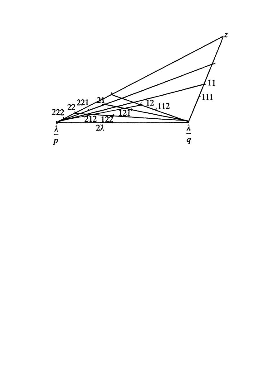
Figure 2.1: Successive transforms of a point $z$, in the case $p=2/3,q=1/3$.

Letting

$$\begin{cases}\displaystyle g_{n}=(-1)^{n}\sum_{\sigma}\exp(-\sigma(0))(p^{n};q^{n})^{\sigma},\\[11.38092pt] \displaystyle k_{n}=(-1)^{n}\sum_{\sigma}\sigma(0)\exp(-\sigma(0))(p^{n};q^{n})^{\sigma},\\[11.38092pt] \displaystyle D(\lambda)=\sum_{n\geq 2}[1-Kn)g_{n}+Kk_{n}]\frac{\lambda^{n}}{n!},\end{cases}$$

we summarize the main results obtained in [7] . Let

$$\mathbf{S}[f(\cdot);z]\stackrel{{\scriptstyle\mbox{\tiny def}}}{{=}}\sum_{\sigma\in H}\big{[}f(\sigma(z))-f(\sigma(0))-(p;q)^{\sigma}zf^{\prime}(\sigma(0))\bigr{]}.$$

Theorem 2.1.

$$\psi(z)=1-\frac{2\,\mathbf{S}[e^{-u}(1+Ku);z]}{1+2D(\lambda)}.$$

Theorem 2.2 (Asymptotics).

The mean time to resolve $n$ collisions satisfies

$$\alpha_{n}=\frac{2A}{1+2D(\lambda)}n+\frac{1}{1+2D(\lambda)}\sum_{\chi}a(\chi)n^{-\chi}+\mathcal{O}(n^{1-\eta}),$$ (2.4)

for any sufficiently small $\eta>0$, where the summation is extended to the $\chi$’s satisfying

$$1-p^{-\chi}-q^{-\chi}=0,\ -1\leqslant\Re(\chi)<-1+\eta,\ \chi\neq-1.$$

The sum in the expression is a bounded fluctuating function, with an amplitude small compared to $nA$, typically less by several orders of magnitude, and the following properties hold.

• $A$ is a complicated constant involving a Riemann-Stieltjes integral with respect to a measure having a nowhere differentiable density.

• If  $\displaystyle\frac{\log p}{\log q}=\frac{d}{r}$ is rational, i.e. with $\gcd(d,r)=1$, then

  $$\alpha_{n}=\frac{2A}{1+2D(\lambda)}n+nP(r\log_{p}n)+o(n^{1-\eta}),$$

  with $P(u)$ a Fourier series of $u$ with mean value $0$. In this case $\displaystyle\lim_{n\to\infty}\alpha_{n}/n$ does not exist.

• If  $\displaystyle\frac{\log p}{\log q}$ is not rational, then the sum in (2.4) is $o(n)$ and $\displaystyle\lim_{n\to\infty}\alpha_{n}/n$ exists.

The main ingredients in the proof of Theorem 2.2 are the exponential approximation [i.e. replace $(1-a)^{n}$ by $\exp(-an)$], together with a skillful use of Mellin’s transforms, yielding the intermediate fundamental proposition.

For $r(u)$ is any continuously differentiable function on $[0,\lambda/q]$, define the Dirichlet series

$$\omega(s)=\sum_{\sigma\in H}r(\sigma(0))(p^{s};q^{s})^{\sigma}.$$

Proposition 2.3.

$$\omega(s) = \frac{1}{(s-1)}\frac{1}{h(p,q)(\frac{\lambda}{q}-\frac{\lambda}{p})}\int_{\lambda/p}^{\lambda/q}r(u)du$$

$$+ \int_{0}^{\lambda/q}r^{\prime}(u)w(u)du+\frac{p\log^{2}p+q\log^{2}q}{h(p,q)(\frac{\lambda}{q}-\frac{\lambda}{p})}+o(s-1),$$

where $h(p,q)\stackrel{{\scriptstyle\mbox{\tiny def}}}{{=}}p\log p^{-1}+q\log q^{-1}$ is the entropy function and $w(u)$ is nowhere differentiable.

Theorem 2.4 (Ergodicity).

A necessary and sufficient condition to have a stable channel, i.e. $\alpha_{n}<\infty,\forall n$ finite, is $\lambda<\lambda_{max}$, where $\lambda_{max}$ is the first positive root of $1+2D(\lambda)=0$. The proof relies on standard results on Markov chains, using the stochastic interpretation of $\psi(\lambda)=[1+2D(\lambda)^{-1}$. When $p=q=1/2,\lambda_{max}=0.3601$.

3 Functional equations of two complex variables

In a probabilistic framework, we consider a piecewise homogeneous random walk with sample paths in $\mathbb{Z}_{+}^{2}$, the lattice in the positive quarter plane. In the strict interior of $\mathbb{Z}_{+}^{2}$, the size of the jumps is $1$, and $\{p_{ij},|i|,|j|\leqslant 1\}$ will denote the generator of the process for this region. Thus a transition $(m,n)\to(m+i,n+j),m,n>0,$ can take place with probability $p_{ij}$, and

$$\sum_{|i|,|j|\leqslant 1}p_{ij}=1.$$

No strong assumption is made about the boundedness of the upward jumps on the axes, neither at $(0,0)$. In addition, the downward jumps on the $x$ [resp. $y$] axis are bounded by $L$ [resp. $M$], where $L$ and $M$ are arbitrary finite integers. The basic problem is to determine the invariant measure $\{\pi_{i,j},i,j\geq 0\}$, the generating function of which satisfies the fundamental FE

$$\boxed{Q(x,y)\pi(x,y)=q(x,y)\pi(x)+\widetilde{q}(x,y)\widetilde{\pi}(y)+\pi_{0}(x,y)},$$ (3.1)

where $x,y$ belong to the complex plane $\mathbb{C}$ with $|x|<1,|y|<1\}$, and

$$\begin{cases}\pi(x,y)=\displaystyle\sum_{i,j\geqslant 1}\pi_{ij}x^{i-1}y^{j-1},\\[14.22636pt] \pi(x)=\displaystyle\sum_{i\geqslant L}\pi_{i0}x^{i-L},\quad\widetilde{\pi}(y)=\sum_{j\geqslant M}\pi_{0j}y^{j-M},\\[14.22636pt] Q(x,y)=\displaystyle xy\Bigg{[}1-\sum_{i,j\in\mathcal{S}}p_{ij}x^{i}y^{j}\Bigg{]},\quad\sum_{i,j\in\mathcal{S}}p_{ij}=1,\\[14.22636pt] q(x,y)=\displaystyle x^{L}\Bigg{[}\sum_{i\geqslant-L,j\geqslant 0}p^{\prime}_{ij}x^{i}y^{j}-1\Bigg{]}\equiv x^{L}(P_{L0}(x,y)-1),\\[14.22636pt] \widetilde{q}(x,y)=\displaystyle y^{M}\Bigg{[}\sum_{i\geqslant 0,j\geqslant-M}p^{\prime\prime}_{ij}x^{i}y^{j}-1\Bigg{]}\equiv y^{M}(P_{0M}(x,y)-1),\\[17.07182pt] \pi_{0}(x,y)=\displaystyle\sum_{i=1}^{L-1}\pi_{i0}x^{i}\big{[}P_{i0}(x,y)-1\big{]}+\sum_{j=1}^{M-1}\pi_{0j}y^{j}\big{[}P_{0j}(x,y)-1\big{]}+\pi_{00}(P_{00}(xy)-1).\end{cases}$$

In equation (3.1), $\mathcal{S}$ is the set of allowed jumps, the unknown functions $\pi(x,y),\pi(x),\widetilde{\pi}(y)$ are sought to be analytic in the region $\{(x,y)\in\mathbb{C}^{2}:|x|<1,|y|<1\}$, and continuous on their respective boundaries. In addition, $q,\widetilde{q},q_{0},P_{i0},P_{0j},$ are given probability generating functions supposed to have suitable analytic continuations (as a rule, they are polynomials when the jumps are bounded).

The polynomial $Q(x,y)$ is often referred to as the kernel of (3.1).

Completely new approaches toward the solution of the problem were discovered by the authors of the book [9], the goal going far beyond the mere obtention of an index theory for the quarter plane. The main results can be summarized as follows.

1. The first step, which is quite similar to a Wiener–Hopf factorization, consists in considering the above equation on the algebraic curve $\{Q(x,y)=0\}$ (which is elliptic in the generic situation), so that we are then left with an equation for two unknown functions of one variable on this curve.

2. Next a crucial idea is to use Galois automorphisms on this algebraic curve. Let $\mathbb{C}\,(x,y)$ be the field of rational functions in $(x,y)$ over $\mathbb{C}$. Since $Q$ is assumed to be irreducible in the general case, the quotient field $\mathbb{C}\,(x,y)$ denoted by $\mathbb{C}_{Q}(x,y)$ is also a field.

   Definition 3.1.

   The group of the random walk is the Galois group $\mathcal{H}=\langle\xi,\eta\rangle$ of automorphisms of $\mathbb{C}_{Q}(x,y)$ generated by $\xi$ and $\eta$ given by

   $$\xi(x,y)=\Bigg{(}x,\frac{1}{y}\frac{\sum_{i}p_{i,-1}x^{i}}{\sum_{i}p_{i,1}x^{i}}\Bigg{)},\ \ \ \ \ \eta(x,y)=\Bigg{(}\frac{1}{x}\frac{\sum_{j}p_{-1,j}y^{j}}{\sum_{j}p_{1,j}y^{j}},y\Bigg{)}.$$

   Here $\xi$ and $\eta$ are involutions satisfying $\xi^{2}=\eta^{2}=I$. Let $\delta\stackrel{{\scriptstyle\mbox{\tiny def}}}{{=}}\eta\xi$ denote their product, which is non-commutative except for $\delta^{2}=I$.Then $\mathcal{H}$ has a normal cyclic subgroup $\mathcal{H}_{0}=\{\delta^{i},i\in\mathbb{Z}\,\}$, which is finite or infinite, and $\mathcal{H}/\mathcal{H}_{0}$ is a group of order $2$. Hence the group $\mathcal{H}$ is finite of order $2n$ if, and only if,

   $$\delta^{n}=I.$$ (3.2)

   More information is obtained by using the fact that the unknown functions $\pi$ and $\widetilde{\pi}$ depend solely on $x$ and $y$ respectively, i.e. they are invariant with respect to $\xi$ and $\eta$ correspondingly. It is then possible to prove that $\pi$ and $\widetilde{\pi}$ can be lifted as meromorphic functions onto the universal covering of some Riemann surface ${\bf S}$. Here ${\bf S}$ corresponds to the algebraic curve $\{Q(x,y)=0\}$. When $g\stackrel{{\scriptstyle\mbox{\tiny def}}}{{=}}$ the genus of ${\bf S}$ is $1$ (resp. $0$), the universal covering is the complex plane $\mathbb{C}$ (resp. the Riemann sphere).

3. Lifted onto the universal covering, $\pi$ (and also $\widetilde{\pi}$) satisfies a system of non-local equations having the simple form

   $$\begin{cases}\pi(t+\omega_{1})=\pi(t),\quad\forall t\in\mathbb{C}\,,\\ \pi(t+\omega_{3})=a(t)\pi(t)+b(t),\quad\forall t\in\mathbb{C}\,,\end{cases}$$

   where $\omega_{1}$ [resp. $\omega_{3}$] is a complex [resp. real] constant. The solution can be presented in terms of infinite series equivalent to Abelian integrals. The backward transformation (projection) from the universal covering onto the initial coordinates can be given in terms of uniformization functions, which, for $g=1$, are elliptic functions.

4. Another direct approach to solving the fundamental equation consists in working solely in the complex plane $\mathbb{C}$. After making the analytic continuation, it appears that the determination of $\pi$ reduces to a boundary value problem (BVP), belonging to the Riemann–Hilbert–Carleman class, the basic form of which can be formulated as follows.

   Let $\mathscr{G}(\mathcal{L})$ denote the interior of the domain bounded by a simple smooth closed contour $\mathcal{L}$.

   Find a function $\Phi^{+}$ holomorphic in $\mathscr{G}(\mathcal{L})$, the limiting values of which are continuous on the contour and satisfy the relation

   $$\Phi^{+}(\alpha(t))=G(t)\Phi^{+}(t)+g(t),\quad t\in\mathcal{L},$$ (3.3)

   where

   • $g$, $G\in\mathbb{H}_{\,\mu}(\mathcal{L})$ (Hölder condition with parameter $\mu$ on $\mathcal{L}$);

   • $\alpha$, referred to as a shift in the sequel, is a function establishing a one-to-one mapping of the contour $\mathcal{L}$ onto itself, such that the direction of traversing $\mathcal{L}$ is changed and

     $$\alpha^{\prime}(t)=\frac{d\alpha(t)}{dt}\in\mathbb{H}_{\,\mu}(\mathcal{L}),\quad\alpha^{\prime}(t)\neq 0,\quad\forall t\in\mathcal{L}.$$

   In addition, the function $\alpha$ is most frequently subject to the so-called Carleman condition

   $$\alpha(\alpha(t))=t,\quad\forall t\in\mathcal{L},\quad\text{where typically}\quad\alpha(t)=\overline{t}.$$

   The advantage of this method resides in the fact that solutions are given in terms of explicit integral-forms.

5. Analytic continuation gives a clear understanding of possible singularities and thus allows to derive the asymptotics of the functions.

All these techniques work quite similarly for Toeplitz operators, and for other questions related to random walks as well: transient behavior, first hitting time problem [GROM73], calculating the Martin boundary, non spatially homogeneous walks, etc.

For the sake of historical reference, it is worth quoting the pioneering work of V.A. Malyshev relating to points $1,2,3$, which was mainly settled in the period 1968–1972 (see e.g., [18, 19, 20]).

The method concerning points $1$ and $4$ was proposed in the seminal study [8] carried out in 1976–1979, which was widely referred to and followed up in many other papers, until today. The three authors joined their efforts in the book [9], where the reader can find a fairly comprehensive bibliography.

3.1 Summary of some general results (see [9])

The multi-valued algebraic function $Y(x)$ solution of the polynomial equation

$$Q(x,Y(x))=0,\quad x\in\mathbb{C},$$

is defined in the $\mathbb{C}_{x}$-plane and has two branches $Y_{0}(x),Y_{1}(x)$. Rewrite for a while $Q(x,y)$ in the form

$$Q(x,y)=a(x)y^{2}+b(x)y+c(x).$$ (3.4)

3.1.1 Genus $1$

In this case, it can be shown that $Y(x)$ has $4$ real branch points, which are the roots of the discriminant $D(x)=b^{2}(x)-4a(x)c(x)$, two of them $x_{1},x_{2}$ being located inside the unit disc $\mathcal{D}$. In addition, there exists a uniformization in terms of the Weierstrass $\wp$ function with periods $\omega_{1},\omega_{2}$ depending on the parameters $p_{ij}$.

Clearly, exchanging $x$ and $y$, similar properties hold for the function $X(y)$ defined by $Q(X(y),y)=0$.

Let $[\underleftarrow{\overrightarrow{x_{1}x_{2}}}]$ stand for the contour $[x_{1}x_{2}]$, traversed from $x_{1}$ to $x_{2}$ along the upper edge of the slit $[x_{1}x_{2}]$ and then back to $x_{1}$, along the lower edge of the slit. Similarly, $[\underrightarrow{\overleftarrow{x_{1}x_{2}}}]$ is defined by exchanging “upper” and “lower”. Noting that on their respective cuts $Y_{0}(x)=\overline{Y}_{1}(x)$ and $X_{0}(y)=\overline{X}_{1}(y)$, one can set

$$\begin{cases}\mathcal{L}&=\ Y_{0}[\underleftarrow{\overrightarrow{x_{1}x_{2}}}]=\overline{Y}_{1}[\underrightarrow{\overleftarrow{x_{1}x_{2}}}],\\ \mathcal{L}_{ext}&=\ Y_{0}[\underleftarrow{\overrightarrow{x_{3}x_{4}}}]=\overline{Y}_{1}[\underrightarrow{\overleftarrow{x_{3}x_{4}}}],\\ \mathcal{M}&=\ X_{0}[\underleftarrow{\overrightarrow{y_{1}y_{2}}}]=\overline{X}_{1}[\underrightarrow{\overleftarrow{y_{1}y_{2}}}],\\ \mathcal{M}_{ext}&=\ X_{0}[\underleftarrow{\overrightarrow{y_{3}y_{4}}}]=\overline{X}_{1}[\underrightarrow{\overleftarrow{y_{3}y_{4}}}].\end{cases}$$

Theorem 3.2 (part of Theorem 5.3.3 in [9]).

1. The curves $\mathcal{L}$ and $\mathcal{L}_{ext}$ (resp. $\mathcal{M}$ and $\mathcal{M}_{ext}$) are simple, closed and symmetrical about the real axis in the $\mathbb{C}_{y}$ [resp. $\mathbb{C}_{x}$] plane. They do not intersect if the group of the random walk is not of order 4. When this group is of order 4, $\mathcal{L}$ and $\mathcal{L}_{ext}$ [resp. $\mathcal{M}$ and $\mathcal{M}_{ext}$] coincide and form a circle possibly degenerating into a straight line. In the general case they build the two components (possibly identical, in which case the circle must be counted twice) of a quartic curve (see an example in figure 3.2).

2. The functions $Y_{i}$ [resp. $X_{i}$], $i=0,1$, are meromorphic in the plane $\mathbb{C}_{x}$ cut along $[x_{1}x_{2}]\cup[x_{3}x_{4}]$ (resp. $\mathbb{C}_{y}$ cut along $[y_{1}y_{2}]\cup[y_{3}y_{4}]$). In addition,

   • $Y_{0}$ [resp. $X_{0}$] has two zeros, no poles, and $|Y_{0}(x)|\leq 1,\ \forall\,|x|=1$.

   • $Y_{1}$ [resp. $X_{1}$] has two poles and no zeros.

   • $|Y_{0}(x)|\leqslant|Y_{1}(x)|$ [resp. $|X_{0}(y)|\leqslant|X_{1}(y)|$], in the whole cut complex plane. Equality holds only on the cuts. $\blacksquare$

Figure 3.2: Example of the mappings of the cuts

Combining the two basic constraints imposed on $\pi$ and $\widetilde{\pi}$ (i.e. they must be holomorphic inside their respective unit disc $\mathcal{D}$ and continuous on the boundary the unit circle), and using the properties of the branches, it is possible to make the analytic continuation of all the functions, starting from the relation

$$q(X_{0}(y),y)\pi(X_{0}(y))+\widetilde{q}(X_{0}(y),y)\widetilde{\pi}(y)+\pi_{0}(X_{0}(y),y)=0,\;y\in\mathbb{C}.$$ (3.5)

Letting now $y$ tend successively to the upper and lower edge of the slit $[y_{1}y_{2}]$, since $\widetilde{\pi}$ is holomorphic in $\mathcal{D}$ and in particular on $[y_{1}y_{2}]$, we can eliminate $\widetilde{\pi}$ in (3.5) to get

$$\pi(X_{0}(y))f(X_{0}(y),y)-\pi(X_{1}(y))f(X_{1}(y),y)=h(y),\;\mbox{for}\;y\in[y_{1}y_{2}],$$

which has exactly the profile announced in (3.3)! The general theory to solve (3.3) can be found in [15, 17]. It involves integral forms and an important quantity called the index, defined as

$$\chi\stackrel{{\scriptstyle\mbox{\tiny def}}}{{=}}\frac{1}{2\pi}[\arg G]_{\mathcal{L}}=\frac{1}{2i\pi}[\log G]_{\mathcal{L}},$$

which is related to the number of existing solutions. We present now the main substance of [9, Theorems 5.4.1, 5.4.3].

Theorem 3.3.

Let us introduce the following two quantities:

$$\delta\stackrel{{\scriptstyle\mbox{\tiny def}}}{{=}}\left\{\begin{array}[]{l}0,\;{\rm if}\;Y_{0}(1)<1\;{\rm or}\;\left\{Y_{0}(1)=1\;{\rm and}\;\dfrac{dq(x,Y_{0}(x))}{dx}_{|x=1}>0\right\},\\[11.38092pt] 1,\;{\rm if}\;Y_{0}(1)=1\;{\rm and}\;\dfrac{dq(x,Y_{0}(x))}{dx}_{|x=1}<0.\end{array}\right.$$

$$\widetilde{\delta}\stackrel{{\scriptstyle\mbox{\tiny def}}}{{=}}\left\{\begin{array}[]{l}0,\;{\rm if}\;X_{0}(1)<1\;{\rm or}\;\left\{X_{0}(1)=1\;{\rm and}\;\dfrac{d\widetilde{q}(X_{0}(y),y)}{dy}_{|y=1}>0\right\},\\[11.38092pt] 1,\;{\rm if}\;X_{0}(1)=1\;{\rm and}\;\dfrac{d\widetilde{q}(X_{0}(y),y)}{dy}_{|y=1}<0.\end{array}\right.$$

Then (3.1) admits a probabilistic solution if, and only if,

$$\delta+\widetilde{\delta}=\leavevmode\hbox{\rm\small 1\kern-3.15005pt\normalsize 1}_{\{X_{0}(1)=1,Y_{0}(1)=1\}}+1,$$ (3.6)

which are the exact conditions for the random walk to be ergodic. $\blacksquare$

Theorem 3.4.

Under the condition (3.6), the function $\pi$ is given by

$$\pi(x)=\frac{U(x)H(x)}{2i\pi}\int_{\mathcal{M}_{d}}{K(t)w^{\prime}(t)dt\over H^{+}(t)(w(t)-w(x))}+V(x),\quad\forall x\in\mathscr{G}(\mathcal{M}),$$ (3.7)

where

1. $\mathscr{G}(\mathcal{M})$ denotes the interior domain bounded by $\mathcal{M}$, and $\mathcal{M}_{d}$ is the portion of the curve $\mathcal{M}$ located in the lower half-plane $\Im z\leqslant 0$;

2. $U,V,K$ are known functions, all involving some specific zeros of $\widetilde{q}(X_{0}(y),y)$ and $q(x,Y_{0}(x))$ inside $G_{\mathcal{M}}$; moreover $U,V$ are rational fractions;

3. $w$ is a gluing function, which realizes the conformal mapping of $\mathscr{G}(\mathcal{M})$ onto the complex plane cut along a segment and has an explicit form via the Weierstrass $\wp$-function;

4. $$H(t) = (w(t)-X_{0}(y_{2}))^{-\widetilde{\chi}}e^{\Gamma(t)},\;t\in\mathscr{G}(\mathcal{M}),$$

   $$\Gamma(t) = {1\over 2i\pi}\int_{\mathcal{M}_{d}}\log{K(\overline{s})\over K(s)}\,{w^{\prime}(s)ds\over w(s)-w(t)},\;t\in\mathscr{G}(\mathcal{M}),$$

   $$H^{+}(t) = (w(t)-X_{0}(y_{2}))^{-\widetilde{\chi}}e^{\Gamma^{+}(t)},\;t\in\mathcal{M}_{d},$$

   $$\Gamma^{+}(t) = {1\over 2}\log{K(\overline{t})\over K(t)}+{1\over 2i\pi}\int_{\mathcal{M}_{d}}\log{K(\overline{s})\over K(s)}\,{w^{\prime}(s)ds\over w(s)-w(t)},\;t\in\mathcal{M}_{d}\;.$$

$\blacksquare$

The detailed proofs of these theorems can be found in the book [9].

3.1.2 Genus $0$

${\bf S}$ has genus $0$ if, and only if, the discriminant $D(x)$ has a multiple zero (possibly at infinity). Hence, we are left with only two branch points in the plane $\mathbb{C}_{x}$ (resp. $\mathbb{C}_{y}$). This situation occurs in the $5$ following cases.

Theorem 3.5.

  The algebraic curve defined by $Q(x,y)=0$ has genus 0 in the following cases.

1. $\begin{cases}x_{1}=x_{2}=0\\ y_{3}=y_{4}=\infty.\end{cases}$   

2. $\begin{cases}y_{1}=y_{2}=0\\ x_{3}=x_{4}=\infty.\end{cases}$   

3. $\begin{cases}x_{3}=x_{4}=\infty\\ y_{3}=y_{4}=\infty.\end{cases}$   

4. $\begin{cases}x_{1}=x_{2}=0\\ y_{1}=y_{2}=0.\end{cases}$   

5. $\begin{cases}x_{2}=x_{3}=1\\ y_{2}=y_{3}=1.\end{cases}$   

In addition $x_{3}$ and $y_{3}$ are always positive, but $x_{4}$ and $y_{4}$ need not be positive. If for instance $x_{4}<0$, then the plane is cut along $[-\infty,x_{4}]\cup[x_{3},+\infty]$.

Figure 3.3: The contour $\mathcal{M}_{1}\cup\mathcal{M}_{2}$, for $r<0$,

$$\mathcal{M}_{1}=X[\overrightarrow{\underleftarrow{y_{1},1}}],\qquad\mathcal{M}_{2}=X[\overrightarrow{\underleftarrow{1,y_{4}}}].$$

$\blacksquare$

$\bullet$ Here the algebraic curve $\{Q(x,y)=0\}$ admits of a rational uniformization by means of rational fractions of degree $2$: that simplifies matters to a certain extent. Indeed, for each of the $5$ cases listed above, conformal mappings (or gluing functions) can be explicitly computed, still allowing to get integrals like in (3.7). For instance, case $3$ leads to a BVP set on an ellipse. In case $1$ (resp. case $2$) $\widetilde{\pi}(y)$ (resp. $\pi(x)$ is rational.

$\bullet$ However, case $5$ corresponds to the so-called zero drift situation $x_{2}=x_{3}=1=y_{2}=y_{3}$ and is a bit more awkward. A BVP can be set on the interior part $\mathcal{M}_{1}$ of the curve shown in figure 3.3, which has a corner point at $x=1$ if, and only if, the correlation coefficient $r$ of the random walk in the interior of the quarter plane is not zero.

4 Examples from queueing systems

We shall describe the outlines of some original models using the above methods.

4.1 Two-coupled processors (see[8, 9])

Consider two parallel M/M/1 queues, with infinite capacities, under the following assumptions.

• Arrivals form two independent Poisson processes with parameters $\lambda_{1},\lambda_{2}$.

• Service times are distributed exponentially with instantaneous service rates $S_{1}$ and $S_{2}$ depending on the state of the system as follows.

  1. If both queues are busy, then $S_{1}=\mu_{1}$ and $S_{2}=\mu_{2}$.

  2. If queue $2$ is empty, then $S_{1}=\mu_{1}^{*}$.

  3. If queue $1$ is empty, then $S_{2}=\mu_{2}^{*}$.

• The service discipline is FIFO (first-in-first-out) in each queue.

One can directly see that the evolution of the system can be described by the two-dimensional continuous time Markov process $(M_{t},N_{t})$, which stands for the joint number of customers in the queues.

Let $p_{t}(m,n)$ the probability $\mathbb{P}(M_{t}=m,N_{t}=n)$ that, at time $t$, one finds $m$ jobs in queue $1$ and $n$ customers in queue $2$. The stationary probabilities

$$p(m,n)\stackrel{{\scriptstyle\mbox{\tiny def}}}{{=}}\lim_{t\to\infty}p_{t}(m,n)$$

satisfy the classical Kolmogorov forward equations, which after setting

$$F(x,y)=\sum_{m\geq 0,n\geq 0}p(m,n)x^{m}y^{n},$$

lead to the basic functional equation (leaving the details to the reader)

$$T(x,y)F(x,y)=a(x,y)F(0,y)+b(x,y)F(x,0)+c(x,y)F(0,0),$$ (4.1)

where

$$\begin{cases}\displaystyle T(x,y)=\lambda_{1}(1-x)+\lambda_{2}(1-y)+\mu_{1}\left(1-\frac{1}{x}\right)+\mu_{2}\left(1-\frac{1}{y}\right),\\[8.5359pt] \displaystyle a(x,y)=\mu_{1}\left(1-\frac{1}{x}\right)+q\left(1-\frac{1}{y}\right),\\[8.5359pt] \displaystyle b(x,y)=\mu_{2}\left(1-\frac{1}{y}\right)+p\left(1-\frac{1}{x}\right),\\[8.5359pt] \displaystyle c(x,y)=p\left(\frac{1}{x}-1\right)+q\left(\frac{1}{y}-1\right),\\[5.69046pt] p=\mu_{1}-\mu_{1}^{*},\\ q=\mu_{2}-\mu_{2}^{*}.\end{cases}$$

Here, there are some pleasant facts. For instance, the two roots of $T(x,y)=0$ satisfy $Y_{0}(x).Y_{1}(x)=\mu_{2}/\lambda_{2}$, which shows that $\widetilde{\pi}(y)$ satisfies a BVP on the circle $\mathbb{C}\bigl{(}\sqrt{\frac{\mu_{2}}{\lambda_{2}}}\bigr{)}$ with simpler formulas. For instance, when $pq=\mu_{1}\mu_{2}$, that is, for $0\leq\xi\leq 1$,

$$\begin{cases}\mu_{1}=\xi\mu_{1}^{*},\\ \mu_{2}=(1-\xi)\mu_{2}^{*},\end{cases}$$ (4.2)

which corresponds to the head of line processor sharing discipline, we have, assuming the ergodicity condition $1-\lambda_{1}/\mu_{1}^{*}-\lambda_{2}/\mu_{2}^{*}>0$,

$$F\left(0,\sqrt{\frac{\mu_{2}}{\lambda_{2}}}z\right)=\frac{1}{\pi}\int_{0}^{\pi}\frac{z\sin{\theta}\,v(\theta)d\theta}{z^{2}-2z\cos{\theta}+1}+F(0,0),\quad|z|<1,$$

where

$$v(\theta) =\frac{-\lambda_{2}\sin{\theta}\,K(\theta)}{\xi[\rho_{1}^{*}(\mu_{2}^{*}-\mu_{1}^{*})K^{2}(\theta)+(\mu_{1}^{*}-\mu_{2}^{*}+\lambda_{1}+\lambda_{2})K(\theta)-\mu_{1}^{*}]},$$

$$K(\theta) =\frac{\lambda_{1}+\mu_{1}+\beta-\sqrt{[(\sqrt{(\lambda_{2}}+\sqrt{\mu_{2}})^{2}+\beta][(\sqrt{\lambda_{2}}-\sqrt{\mu_{2}})^{2}+\beta]}}{2\lambda_{1}},$$

$$\beta =\lambda_{2}+\mu_{2}-2\sqrt{\lambda_{2}\mu_{2}}\cos{\theta}.$$

In [8], the functions $F(0,y)$ and $F(x,0)$ have been completely expressed in terms of elliptic integrals of the third kind.

4.2 Sojourn time in a Jackson network with overtaking (see[10, 9])

A problem analyzed in [10] deals with the sojourn time of a customer in the open 3-node queueing network (of Jackson’s type) shown in figure 4.4. An inherent overtaking phenomenon renders things slightly more complicated. Let us just say that cutting the Gordian Knot amounts to finding the function $G(x,y,z,s)$, which is the Laplace transform of the conditional waiting time distribution of a tagged customer at a departure instant of the first queue. The following non-homogeneous functional equation can be obtained, for $|x|,|y|,|z|\leq 1,\Re(s)\geq 0$,

$$K(x,y,z,s)G(x,y,z,s) =\left(\mu_{1}-\dfrac{\lambda}{x}\right)G(0,y,z,s)+\left(\mu_{3}-q\mu_{1}\dfrac{x}{z}-\mu_{2}\dfrac{y}{z}\right)G(x,y,0,s)$$

$$+\dfrac{\mu_{2}\mu_{3}}{(1-x)[s+\mu_{3}(1-z)]},$$

where $p,q$ are routing probabilities with $p+q=1$, $\lambda$ is the external arrival rate, $\mu_{i}$ is the service rate at queue $i$, and

$$K(x,y,z,s)=s+\lambda\left(1-\dfrac{1}{x}\right)+\mu_{1}\left(1-px-q\dfrac{x}{z}\right)+\mu_{2}\left(1-\dfrac{y}{z}\right)+\mu_{3}(1-z).$$

Then, considering $y$ and $s$ as parameters, the last equation takes the form

$$\boxed{K(x,y,z,s)\widetilde{G}(x,z)=A(x)\widetilde{G}(0,z)+B(x,y,z,s)\widetilde{G}(x,0)+C(x,y,z,s)},$$

where $K,A,B,C$ are known functions. The reduction to a BVP is carried out according to the general methodology. Finally, setting $\rho_{i}=\lambda/\mu_{i}$, and using the geometic form of the steady state distribution for the number of customers, it follows (see [10]) that the total sojourn time of an arbitrary customer has a Laplace transform given by

$$(1-\rho_{1})(1-\rho_{2})(1-\rho_{3})\frac{\mu_{1}}{\mu_{1}+s}G\left[\frac{\mu_{1}}{\mu_{1}+s},\rho_{2},\rho_{3},s\right].$$

Figure 4.4: Network with overtaking

4.3 Two queues with alternative service periods (see [4])

Consider a system of two queues, $Q_{1}$ and $Q_{2}$, and a single server that alternates service between them. (See figure 4.5) When customers are being served in $Q_{i}$, the system behaves as an M/M/l queue with arrival and service rate parameters $\lambda_{i}$ and $\mu_{i}$ ($i=1,2$), respectively. The interarrival and service times in $Q_{1}$ are independent of those in $Q_{2}$.

Service is alternated in such a way as to limil the lime spent by the server away from a nonemply queue. If both queues are empty the server simply idles; it immediately begins service at the queue where the next arrivai occurs. When service begins at a non-empty $Q_{1}$, a timer is started with the initial value $T_{1}$. Customers in $Q_{1}$ are then served until eilher none remain or the $T_{1}$ time units have elapsed, whichever occurs first. If at this later lime, $Q_{2}$ is empty but $Q_{1}$ is still non-empty, then the above procedure is repeated; however, if $Q_{2}$ is non-emply then the server begins serving customers in $Q_{2}$. Service of customers in $Q_{2}$ is similar to thal in $Q_{1}$; the initial timer value is now $T_{2}$, and a return to $Q_{1}$ from $Q_{2}$ does not occur while $Q_{1}$ is emply. The analysis is based on the assumption lhat $T_{1}$ and $T_{2}$ arc independcnt samples from exponential distributions wilh parameters $\xi_{1}$ and $\xi_{2}$ respcctively.

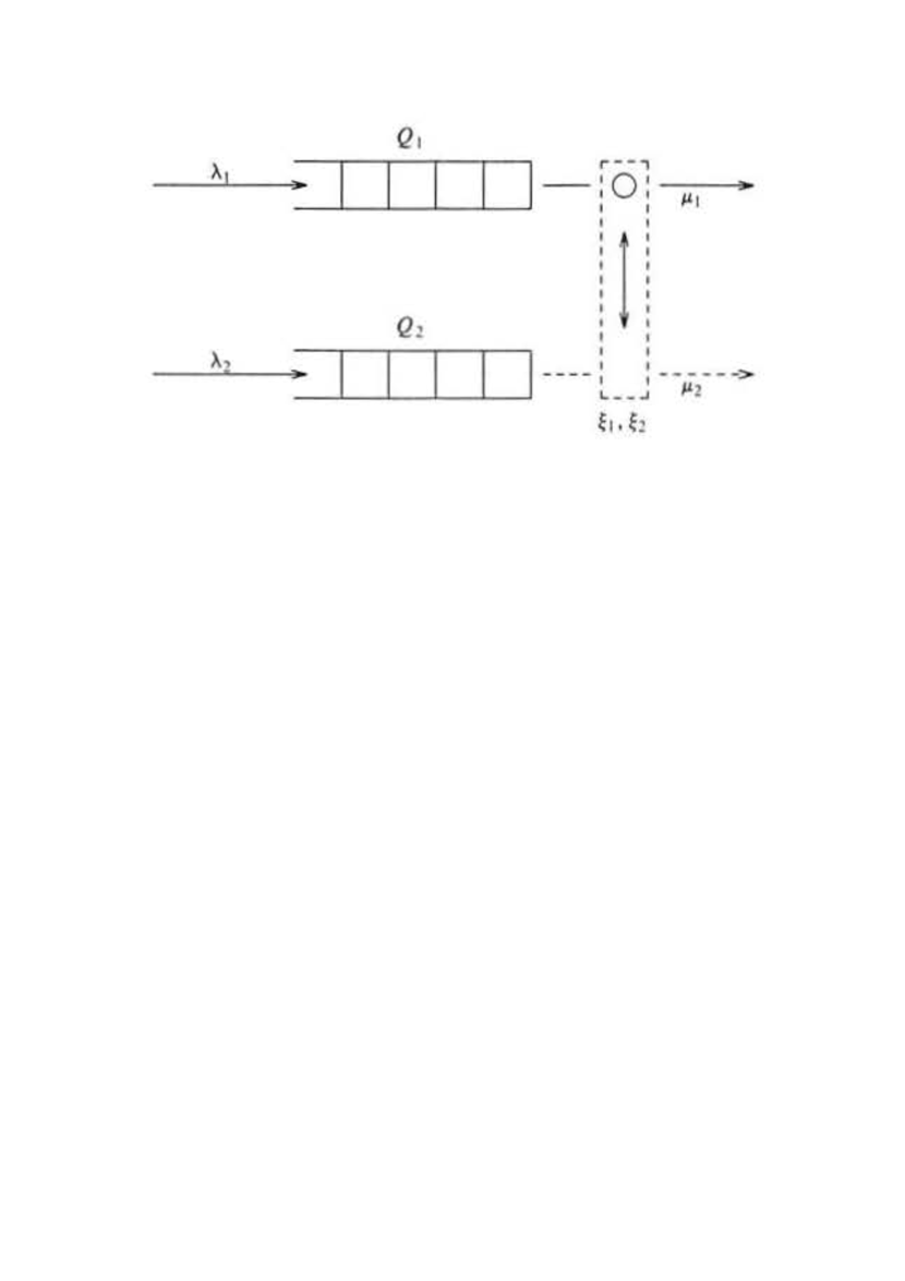
Figure 4.5: Two queues with alternative service periods

For $l=1,2$ , we define the state probabilities

$$p_{l}(i,j)=\mathbb{P}(\mathrm{server\ at}\ Q_{l},i\ \mathrm{customers\ in\ }Q_{1},j\ \mathrm{customers\ in\ Q_{2}}),$$

with $p(0,0)=p_{1}(0,0)=p_{2}(0,0)$. Then it is convenient to work with the generating functions

$$G_{1}(x,y)=\sum_{i\geq 1,j\geq 0}p_{1}(i,j)x^{i-1}y^{j},\quad G_{2}(x,y)=\sum_{i\geq 0,j\geq 1}p_{2}(i,j)x^{i}y^{j-1}.$$

The ergodicity condition $\rho_{1}+\rho_{2}<1$, where $\rho_{i}=\lambda_{i}/\mu_{i}$, can be easily derived by comparison with an M/G/1 queue and will be assumed to hold.

Here we end up with a system of two FEs involving a priori four unknown functions $G_{l}(0,y),G_{l}(x,0)$, which are easily reduced to two by simple manipulations.

Let

$$\begin{cases}\displaystyle R_{1}(x,y)=\lambda_{1}(1-x)+\lambda_{2}(1-y)+\mu_{1}\bigl{(}1-\frac{1}{x}\bigr{)},\\[5.69046pt] \displaystyle R_{2}(x,y)=\lambda_{1}(1-x)+\lambda_{2}(1-y)+\mu_{2}\bigl{(}1-\frac{1}{y}\bigr{)},\\[8.5359pt] \displaystyle\Delta(x,y)=(R_{1}(x,y)+\xi_{1})(R_{2}(x,y)+\xi_{2})-\xi_{1}\xi_{2},\\[5.69046pt] \displaystyle H(x)=x(R_{1}(x,0)+\xi_{1})G_{1}(x,0),\\[5.69046pt] \displaystyle K(y)=y(R_{2}(0,y)+\xi_{2})G_{2}(0,y)+\mu_{2}G_{2}(0,0)-p(0,0)\lambda_{2}y,\\[5.69046pt] \displaystyle g(x,y)=\frac{\lambda_{1}(1-x)+\lambda_{2}(1-y)}{R_{2}(x,y)}\xi_{2}p(0,0).\end{cases}$$

Omitting some tiresome algebra, the following FE of type (3.1) can be obtained.

Lemma 4.1.

For $\Delta(x,y)=0$, with $|x|\leq 1$ and $|y|\leq 1$, we have

$$H(x)-K(y)=g(x,y).$$ (4.3)

$\blacksquare$

Assume the polynomial $xy\Delta(x,y)$ to be irreducible. In this case, the Riemann surface ${\bf S}$ corresponding to $\Delta(x,y)=0$ is in general of genus greater than $1$, as it reduces to a polynomial equation of degree $3$ in $x$ and in $y$ ($3$-sheeted covering). However, there still exists a real cut, say $[x_{1},x_{2}]$, in the unit disc of the $\mathbb{C}_{x}$ plane, so that a BVP of Dirichlet type (i.e. without coefficient) can be defined. Then $H(x)$ is given by a Cauchy type integral, the density of which satisfies a Fredholm integral equation. The hassle is the analysis of the branch points: this requires to deal with a polynomial of degree $11\,!$. Luckily enough, a computationally more efficient solution can be obtained via the following approach.

4.3.1 Mixing uniformization and BVP

As the uniformizalion step, we put

$$R_{1}(x,y)+\xi_{1}=\xi_{1}z,\qquad R_{2}(x,y)+\xi_{2}=\frac{\xi_{2}}{z}.$$ (4.4)

Hence $\Delta(x,y)=0$ for $x,y$ such that (4.4) holds. Setting $\lambda=\lambda_{1}+\lambda_{2}$ and

$$\nu=r_{1}x+r_{2}y,$$

where $r_{i}=\lambda_{i}/\lambda$, we relate $(x,y)$ to $(\nu,z)$ by

$$x(\nu,z)=\frac{\mu_{1}}{\mu_{1}+\lambda(1-\nu)+\xi_{1}(1-z)},\qquad y(\nu,z)=\frac{\mu_{2}}{\mu_{2}+\lambda(1-\nu)+\xi_{2}(1-\frac{1}{z})},$$ (4.5)

with

$$\nu=\frac{r_{1}\mu_{1}}{\mu_{1}+\lambda(1-\nu)+\xi_{1}(1-z)}+\frac{r_{2}\mu_{2}}{\mu_{2}+\lambda(1-\nu)+\xi_{2}(1-\frac{1}{z})}.$$ (4.6)

Lemma 4.2.

1. For any $z$ with $|z|=1$, there exists exactly one $\nu=\nu(z)$ such that $|v|\leq 1$ and $\Delta(x,y)=0$, with $|x|,|y|\leq 1,\,x=x(v,z),\,y=y(v,z)$. For $z=1$, this value is $v=1$.

2. Let $|\nu|=1$ and $\xi_{1}\rho_{1}\geq\xi_{2}\rho_{2}$. Then (4.6) has exactly one root $z(\nu)$ satisfying $|z|\geq 1$; the equality $|z|=1$ holds only for $\nu=z(\nu)=1$.

$\blacksquare$

The proof of Lemma 4.2 is direct by Rouché’s theorem and the principle of the argument.

The behaviour of the functions $\nu(z)$ and $z(\nu)$ is illustrated in figure 4.6. The unit circle $|z|=1$ is mapped by $\nu(z)$ onto the closed contour $\Gamma_{\nu}$ lying entirely within the unit circle $\nu=1$, but touching it at $\nu=1$. The unit circle $|\nu|=1$ is mapped by $z(\nu)$ onto a closed contour $\Gamma_{z}$ lying entirely outside and to the right of $|z|=1$, but touching it at $z=1$. The region between $|\nu|=1$ and $\Gamma_{\nu}$ in the $\nu$-plane maps conformally onto a region outside the closed contours $|z|=1$ and $\Gamma_{z}$ (the latter region is not the entire region, but it does include the point al infinity). The figure also shows that the other root, say $\bar{z}(\nu)$ of (4.6) maps $|\nu|=1$ onto a contour wholly inside $|z|=1$; this contour does not touch $z=1$.

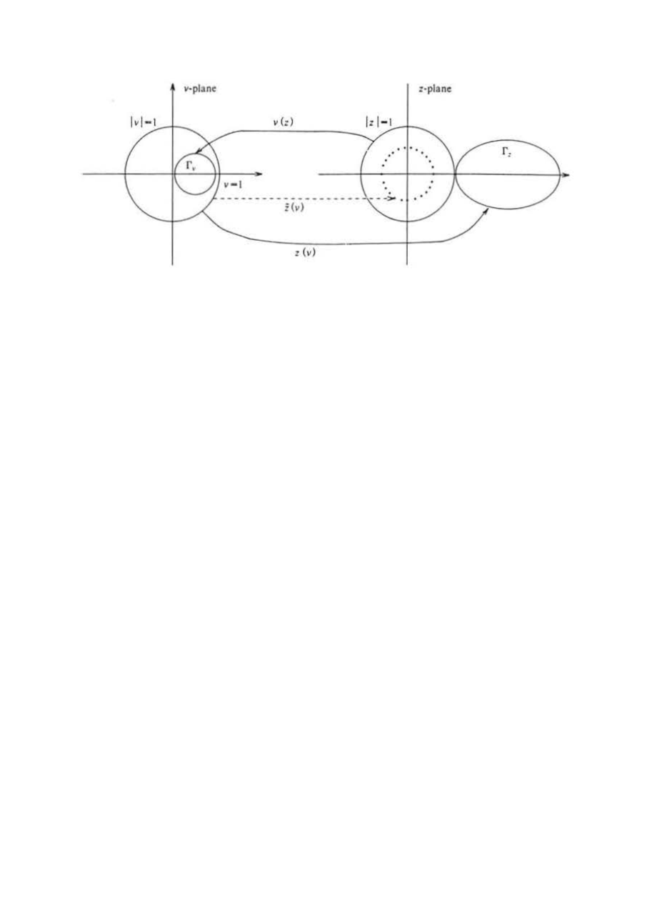
Figure 4.6: The mappings $\nu(z)$ and $z(\nu)$

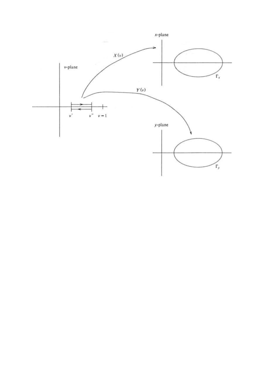
Figure 4.7: The mappings $X(\nu)$ and $Y(\nu)$

Writing $X(\nu)\stackrel{{\scriptstyle\mbox{\tiny def}}}{{=}}X(\nu,z(\nu))$ and $Y(\nu)\stackrel{{\scriptstyle\mbox{\tiny def}}}{{=}}Y(\nu,z(\nu))$, we note that in (4.6) the desired simplification has been realized, from a cubic in $y$ (or $x$) to a quadratic in $z$.

Then, $z(\nu)$ has two (real) branch points $\nu^{\prime}<\nu^{\prime\prime}$ in the unit circle $|\nu|=1$. As $\nu$ moves around the cut $[\nu^{\prime}<\nu^{\prime\prime}]$, $X(\nu)$ and $Y(\nu)$ traverse simple closed contours $\Gamma_{x}$ and $\Gamma_{y}$ in their respective planes $\mathbb{C}_{x}$ and $\mathbb{C}_{y}$, as shown in figure 4.7. With some effort, it can also be proved that the point $y=1$ belongs to the finite region bounded by $\Gamma_{y}$, in which $K(y)$ has no pole. However, the point $x=1$ is not necessarily contained in $\Gamma_{x}$. Rewriting now (4.3) as

$$H(X(\nu))-K(Y(\nu))=f(\nu),$$ (4.7)

where $\displaystyle f(\nu)=\frac{\lambda p(0,0)(1-\nu)z(\nu)}{1-z(\nu)}$, $H(x)$ and $K(y)$ can be analytically continued.

The main lines of solution (which do not need conformal mappings onto the unit disk – see [4] for the details) are sketched below.

First, write the Cauchy type integrals

$$H(x)=\frac{1}{2i\pi}\int_{\Gamma_{x}}\frac{H(t)dt}{t-x},\qquad K(y)=\frac{1}{2i\pi}\int_{\Gamma_{y}}\frac{K(t)dt}{t-y}.$$

Then, let $x$ approach a point of the contour $\Gamma_{x}$, make the change of variables $t=Y(s)$, and use the Plemelj-Sokhotski formulas (see e.g., [15]) to get

$$\frac{1}{2}H(X(\nu))=\frac{1}{2i\pi}\int_{L}\frac{H(X(s))X^{\prime}(s)ds}{X(s)-X(\nu)},\quad\forall\nu\in L\stackrel{{\scriptstyle\mbox{\tiny def}}}{{=}}{[\underleftarrow{\overrightarrow{\nu^{\prime},\nu^{\prime\prime}}}]}.$$

Similarly,

$$\frac{1}{2}K(Y(\nu))=\frac{1}{2i\pi}\int_{\bar{L}}\frac{K(Y(s))Y^{\prime}(s)ds}{Y(s)-Y(\nu)},\quad\forall\nu\in\bar{L}\stackrel{{\scriptstyle\mbox{\tiny def}}}{{=}}{[\underrightarrow{\overleftarrow{\nu^{\prime},\nu^{\prime\prime}}}]},$$

noting that $L$ and $\bar{L}$ are described in opposite directions. Then (4.7) leads to

$$K(y)=\frac{1}{2i\pi}\int_{L}\frac{\psi(s)Y^{\prime}(s)ds}{Y(s)-y},$$

where $\psi(s)$ satisfies the non singular Fredholm integral equation (which can be shown to admit a unique solution by the Fredholm alternative)

$$\psi(s)-\frac{1}{2i\pi}\int_{L}\psi(s)\frac{\partial}{\partial s}\log\frac{X(s)-X(\nu)}{Y(s)-Y(\nu)}ds=\frac{1}{2i\pi}\int_{L}f(s)\frac{\partial}{\partial s}\log\frac{X(s)-X(\nu)}{s-\nu}ds.$$

Obviously, $H(x)$ is directly obtained from (4.3).

4.4 Joining the shorter queue

This example is a long-standing problem borrowed from queueing theory. It highlights the huge additional complexity which arises when space-homogeneity is only partial, even for $2$-dimensional systems. The detailed analysis can be found in [9, Chapter [10].

4.4.1 Equations

Two queues with exponentially distributed service times of rate $\alpha,\beta$, respectively are placed in parallel. The external arrival process is Poisson with parameter $\lambda$. The incoming customer always joins the shorter line, or, if the lines are equal, he joins queue $1$ or queue $2$ with respective probabilities $\pi_{1}$ and $\pi_{2}$. The basic problem is to analyze the steady state distribution of the joint number of customers in the system.

Letting $p_{t}(m,n)$ denote the probability $\mathbb{P}(M_{t}=m,N_{t}=n)$ that at time $t$ there are $m$ customers in queue $1$ and $n$ customers in queue $2$, Kolmogorov’s equations for the stationary probabilities

$$p(m,n)\stackrel{{\scriptstyle\mbox{\tiny def}}}{{=}}\lim_{t\to\infty}p_{t}(m,n)$$

have to be written separately in the two distinct regions

$$\mathcal{R}_{1}\stackrel{{\scriptstyle\mbox{\tiny def}}}{{=}}\{(m,n),m\leq n\}\quad\mbox{and}\quad\mathcal{R}_{2}\stackrel{{\scriptstyle\mbox{\tiny def}}}{{=}}\{(m,n),n\leq m\}.$$

Define

$$\begin{cases}\displaystyle F_{1}(x,y)=\sum_{i,j\geq 0}p(i,i+j)x^{i}y^{j},\quad P_{1}(x)=\sum_{i,\geq 0}p(i,i+1)x^{i},\\[14.22636pt] \displaystyle F_{2}(x,y)=\sum_{i,j\geq 0}p(i+j,i)x^{i}y^{j},\quad P_{2}(x)=\sum_{i,\geq 0}p(i+1,i)x^{i},\\[2.84544pt] \displaystyle Q(x)=F_{1}(x,0)=F_{2}(x,0)=\sum_{i,\geq 0}p(i,i)x^{i},\\[8.5359pt] \displaystyle A_{1}(x)=(\alpha+\lambda x)P_{2}(x),\quad A_{2}(x)=(\beta+\lambda x)P_{1}(x),\\[5.69046pt] \displaystyle G_{i}(y)=F_{i}(0,y),\ i=1,2,\\[5.69046pt] T_{1}(x,y)=\lambda\left(1-\dfrac{x}{y}\right)+\alpha\left(1-\dfrac{y}{x}\right)+\beta\left(1-\dfrac{1}{y}\right),\quad R_{1}(x,y)=xy\,T_{1}(x,y),\\[8.5359pt] T_{2}(x,y)=\lambda\left(1-\dfrac{x}{y}\right)+\beta\left(1-\dfrac{y}{x}\right)+\alpha\left(1-\dfrac{1}{y}\right),\quad R_{2}(x,y)=xy\,T_{2}(x,y),\\[8.5359pt] s=\lambda+\alpha+\beta.\end{cases}$$

Then, some direct algebra yields the following system.

$$\begin{cases}T_{1}(x,y)F_{1}(x,y)&=\alpha\left(1-\dfrac{y}{x}\right)G_{1}(y)+\left(\dfrac{\lambda\pi_{2}y^{2}-\lambda x-\beta}{y}\right)Q(x)+A_{1}(x),\\[8.5359pt] T_{2}(x,y)F_{2}(x,y)&=\beta\left(1-\dfrac{y}{x}\right)G_{2}(y)+\left(\dfrac{\lambda\pi_{1}y^{2}-\lambda x-\alpha}{y}\right)Q(x)+A_{2}(x),\\[8.5359pt] sQ(x)&=A_{1}(x)+A_{2}(x).\end{cases}$$ (4.8)

4.4.2 Reduction of the number of unknown functions

The ergodicity of the process is equivalent to the existence of $F_{1}(x,y)$ and $F_{2}(x,y)$ holomorphic in $\mathcal{D}\times\mathcal{D}$ and continuous in $\overline{\mathcal{D}}\times\overline{\mathcal{D}}$. At first sight, system (4.8) includes four unknown functions of one variable. In fact, this number immediately boils down to two, by using the zeros of the kernels $R_{j}(x,y),j=1,2,$ in $\overline{\mathcal{D}}\times\overline{\mathcal{D}}$. So, we are left with two unknown functions of one complex variable, say for instance $G_{i}(\cdot),i=1,2$, or $A_{i}(.),i=1,2$. In order to get additional information, we can combine several BVPs derived from system (4.8). As we shall see, determining one function is sufficient to find all the others.

4.4.3 Meromorphic continuation to the complex plane

It is easy to check that the algebraic curves defined by $\{R_{j}(x,y)=0\},j=1,2$, correspond to random walks of genus $0$, case $3$ of Theorem 3.5.

Notation and Assumption

For convenience and to distinguish between the two kernels, we shall add, either in a superscript or subscript position ad libitum, the pair $\alpha\beta$ (resp. $\beta\alpha$) to any quantity related to the kernel $R_{1}(x,y)$ (resp. $R_{2}(x,y)$). For instance, the branches $Y_{0}^{\alpha\beta},X_{1}^{\alpha\beta}$, etc. Also, if a property holds both for ${\alpha\beta}$ and ${\beta\alpha}$, the pair is omitted. From now on, we assume $\beta>\alpha$, the case $\beta=\alpha$ being considered in a separate section.

The functions $Y_{i}^{\alpha\beta}(x),i=0,1$, have exactly two branch points, which are always located inside $\mathcal{D}$,

$$x=0,\quad\mathrm{and}\quad x_{\alpha\beta}^{*}=\frac{4\alpha\beta}{s^{2}-4\alpha\lambda}<1.$$ (4.9)

With the notation of Section 3.1.1 for the contour corresponding to a slit, $\Psi^{\alpha\beta}$ will denote the ellipse obtained by the mapping

$$[\underrightarrow{\overleftarrow{0,x^{*}_{\alpha\beta}}}]\ \overset{Y^{\alpha\beta}}{\longrightarrow}\ \Psi^{\alpha\beta}.$$

Note that $\beta>\alpha\iff x_{\alpha\beta}^{*}<x_{\beta\alpha}^{*}$. In the $\mathbb{C}_{y}$-plane, setting $y=u+iv$, the equation of $\Psi^{\alpha\beta}$ is

$$\left(u-\frac{\beta s}{s^{2}-4\alpha\lambda}\right)^{2}+\frac{s^{2}v^{2}}{s^{2}-4\alpha\lambda}=\frac{\beta^{2}s^{2}}{(s^{2}-4\alpha\lambda)^{2}}.$$

Similarly for $X_{i}^{\alpha\beta}(x),i=0,1$, with the branch-points

$$y_{1}^{\alpha\beta}=\dfrac{\beta}{s+2\sqrt{\alpha\lambda}}\ <\ y_{2}^{\alpha\beta}=\dfrac{\beta}{s-2\sqrt{\alpha\lambda}},\quad 0<y_{1}^{\alpha\beta}<y_{2}^{\alpha\beta}<1,$$

and $\Phi^{\alpha\beta}$ will denote the ellipse obtained by the mapping

$$[\underrightarrow{\overleftarrow{y_{1}^{\alpha\beta},y_{2}^{\alpha\beta}}}]\ \overset{X^{\alpha\beta}}{\longrightarrow}\ \Phi^{\alpha\beta}.$$

In the $\mathbb{C}_{x}$-plane, setting $x=u+iv$, the equation of $\Phi^{\alpha\beta}$ is

$$\left(u-\frac{2\alpha\beta}{s^{2}-4\alpha\lambda}\right)^{2}+\frac{s^{2}v^{2}}{s^{2}-4\alpha\lambda}=\frac{\alpha\beta^{2}s^{2}}{\lambda(s^{2}-4\alpha\lambda)^{2}}.$$

Exchanging the parameters $\alpha$ and $\beta$, the respective branch points of $Y_{i}^{\beta\alpha}(x)$ are

$$x=0,\quad\mathrm{and}\quad x_{\beta\alpha}^{*}=\frac{4\alpha\beta}{s^{2}-4\beta\lambda}<1,$$ (4.10)

and those of $X_{i}^{\beta\alpha}(x)$,

$$y_{1}^{\beta\alpha}=\dfrac{\alpha}{s+2\sqrt{\beta\lambda}}\ <y_{2}^{\beta\alpha}=\dfrac{\alpha}{s-2\sqrt{\beta\lambda}},\quad 0<y_{1}^{\beta\alpha}<y_{2}^{\beta\alpha}<1.$$

Theorem 4.3.

The functions $Q(\cdot),G_{i}(\cdot),A_{i}(\cdot),i=1,2,$ can be continued as meromorphic functions to the whole complex plane. $\blacksquare$

The proof (first established in 1979) can be found in [9] and relies on the following lemma.

Lemma 4.4.

Let $\mathcal{D}_{n}$ be the domain recursively defined by

$$\begin{cases}\mathcal{D}_{0}&\!\!=\ \mathcal{D},\\ \mathcal{D}_{n+1}&\!\!=\inf{\left\{(X_{1}\circ Y_{1})^{\alpha\beta}(\mathcal{D}_{n}),(X_{1}\circ Y_{1})^{\beta\alpha}(\mathcal{D}_{n})\right\}}.\end{cases}$$

Then $\mathcal{D}_{n}\subset\mathcal{D}_{n+1}$ and $\displaystyle\lim_{n\to\infty}\mathcal{D}_{n}=\mathbb{C}$, where $\mathbb{C}$ denotes the complex plane. $\blacksquare$

4.4.4 Functional equation for $G_{1}(y)$ and integral equation for $Q(x)$

Hereafter, we shall list the main results of this study, presented in the form of a global Proposition. Proofs involve sharp technicalities are omitted. They can be found in [9] and references therein.

Let

$$\begin{cases}\Delta(x)&=s-\left(\frac{\alpha}{x}+\lambda\pi_{2}\right)Y_{0}^{\alpha\beta}(x)-\left(\frac{\beta}{x}+\lambda\pi_{1}\right)Y_{0}^{\beta\alpha}(x),\\[8.5359pt] K_{1}(z)&=\dfrac{\biggl{(}1-\dfrac{Y_{0}^{\alpha\beta}(z)}{z}\biggr{)}\Delta_{1}(z)}{\biggl{(}1-\dfrac{Y_{0}^{\beta\alpha}(z)}{z}\biggr{)}W^{\alpha\beta}(z)},\quad L_{1}(z)=\dfrac{\biggl{(}1-\dfrac{Y_{1}^{\alpha\beta}(z)}{z}\biggr{)}\Delta(z)}{\biggl{(}1-\dfrac{Y_{0}^{\beta\alpha}(z)}{z}\biggr{)}W^{\alpha\beta}(z)},\\[28.45274pt] \Delta_{1}(z)&=s-\left(\dfrac{\alpha}{z}+\lambda\pi_{2}\right)Y_{1}^{\alpha\beta}(z)-\left(\dfrac{\beta}{z}+\lambda\pi_{1}\right)Y_{0}^{\beta\alpha}(z).\end{cases}$$

Proposition 4.5.

The two functions $G_{1}(y)$ and $Q(x)$ have the following properties.

1. $$\boxed{\begin{aligned} \hbox to0.0pt{$\displaystyle L_{1}(z)G_{1}(Y_{1}^{\alpha\beta}(z))-L_{1}(\bar{z})G_{1}(Y_{1}^{\alpha\beta}(\bar{z}))\ =$\hss}\\ &K_{1}(z)G_{1}(Y_{0}^{\alpha\beta}(z))-K_{1}(\bar{z})G_{1}(Y_{0}^{\beta\alpha}(\bar{z})),\ z\in\Phi^{\beta\alpha}\end{aligned}}\,,$$ (4.11)

   which is equivalent to a generalized Riemann-Carleman BVP on the closed contour $\mathcal{L}=Y_{1}^{\alpha\beta}(\Phi^{\beta\alpha})$, having a unique solution analytic in $\mathcal{D}$ if and only if

   $$\Delta^{\prime}(1)>0,\quad\mbox{\emph{or equivalently}}\ \lambda<\alpha+\beta.$$

   Moreover, under the above ergodicity condition, the whole system (4.8) has also an analytic solution in $\mathcal{D}$.

2. Equation (4.11) reduces to a BVP of the form

   $$\boxed{U^{+}(t)-U^{-}(t)=H(t)\overline{U^{+}(t)}+C,\quad t\in w(\Phi^{\alpha\beta})}\,,$$ (4.12)

   where $H(t)$ is known, and $w(z)$ is a conformal gluing of the domain inside the ellipse $\Phi^{\alpha\beta}$ onto the complex plane cut along an open smooth arc. Moreover, (4.12) defines a Noetherian operator with index $0$, that is a Fredholm operator.

3. For $y\in\mathbb{C}_{y}$, the function $G_{1}(y)$ satisfies the non local FE

   $$\boxed{\begin{aligned} \hbox to0.0pt{$\displaystyle L_{1}(X_{0}^{\beta\alpha}(y))G_{1}(Y_{1}^{\alpha\beta}\circ X_{0}^{\beta\alpha}(y))-L_{1}(X_{1}^{\beta\alpha}(y))G_{1}(Y_{1}^{\alpha\beta}\circ X_{1}^{\beta\alpha}(y))\ =$\hss}\\ &K_{1}(X_{0}^{\beta\alpha}(y))G_{1}(Y_{0}^{\alpha\beta}\circ X_{0}^{\beta\alpha}(y))-K_{1}(X_{1}^{\beta\alpha}(y))G_{1}(Y_{0}^{\alpha\beta}\circ X_{1}^{\beta\alpha}(y))\end{aligned}}\,.$$ (4.13)

4. The function $Q(x)$ satisfies the real integral equation

   $$\boxed{Z(x)Q(x)=\int_{0}^{x^{*}_{\beta\alpha}}Q(u)S(x,u)du+W(x),\quad\forall x\in[0,x^{*}_{\beta\alpha}]}\,,$$ (4.14)

   where $Z(x),S(x,u),W(x)$ are known quantities. $\blacksquare$

Some facts have to be stressed.

• All the unknown functions appearing in system (4.8) can be determined once $Q(.)$ is known.

• From (4.13), explicit (but intricate) recursive computations of the poles and residues of $G_{1}(\cdot)$ can be achieved (see [5]).

• The integral equation (4.14) contains both a regular part and a singular part.

4.5 Explicit integral forms for equal service rates ($\alpha=\beta$)

In this case, the problem simplifies in a breathtaking way ! Indeed, the two kernels $T_{i}(x,y),i=1,2,$ are equal. Using the same objects as before (and omitting the indices ${\alpha\beta}$ or ${\beta\alpha}$), we put

$$\begin{cases}F(x,y)=F_{1}(x,y)+F_{2}(x,y),\\[5.69046pt] G(x,y)=G_{1}(x,y)+G_{2}(x,y),\\[5.69046pt] \Delta(x,y)=s-\left(\dfrac{2\alpha}{x}+\lambda\right)y,\end{cases}$$

Then, from system (4.8), we get the reduced functional equation

$$F(x,y)T(x,y)=\alpha\left(1-\dfrac{y}{x}\right)G(y)-\Delta(x,y)Q(x).$$ (4.15)

the resolution of which (4.15) is straightforward by applying the methods previously discussed. The result is presented in the following proposition without further comment.

Proposition 4.6.

When $\alpha=\beta$, the system is ergodic if and only if $\lambda<2\alpha$, and in this case

$$Q(x)=K\,e^{\Gamma(x)},$$ (4.16)

$$\begin{cases}\Gamma(x)&=\displaystyle\dfrac{1}{2i\pi}\int_{\Phi}\dfrac{\log{w(t)}\theta^{\prime}(t)dt}{\theta(t)-\theta(x)},\quad x\in\mathscr{G}(\Phi),\\[14.22636pt] w(t)&=\dfrac{\overline{i\xi(t)}}{i\xi(t)},\quad\xi(t)=\dfrac{\Delta(t)}{1-\frac{Y_{0}(t)}{t}},\quad\Delta(t)=\Delta(t,Y_{0}(t)),\end{cases}$$

where $K$ is a positive constant, $\mathscr{G}(\Phi)$ is the interior domain bounded by the ellipse $\Phi$, and $\theta(.)$ denotes the conformal mapping of $\mathscr{G}(\Phi)$ onto the unit disc.

5 Counting lattice walks in the quarter plane

Enumeration of planar lattice walks has become a classical topic in combinatorics. For a given set $\mathcal{S}$ of allowed jumps (or steps), it is a matter of counting the number of paths starting from some point and ending at some arbitrary point in a given time, and possibly restricted to some regions of the plane.

Then three important questions naturally arise.

• How many such paths exist?

• What is the nature of the associated counting generating function (CGF) of the numbers of walks? Is it holonomic, and, in that case, algebraic or even rational?

• What is the asymptotic behavior, as their length goes to infinity, of the number of walks ending at some given point or domain (for instance one axis)?

If the paths are not restricted to a region, or if they are constrained to remain in a half-plane, the CGFs have an explicit form and can only be rational or algebraic (see [3]). The situation happens to be much richer if the walks are confined to the quarter plane $\mathbb{Z}_{+}^{2}$.

So, we shall focus on walks confined to $\mathbb{Z}_{+}^{2}$, starting at the origin and having small steps. This means exactly that the set $\mathcal{S}$ of admissible steps is included in the set of the eight nearest neighbors, i.e., $\mathcal{S}\subset\{-1,0,1\}^{2}\setminus\{(0,0)\}$. By using an extended Kronecker’s delta, we shall write

$$\delta_{i,j}=\left\{\begin{array}[]{ccc}1&\text{if}&(i,j)\in\mathcal{S},\\ 0&\text{if}&(i,j)\notin\mathcal{S}.\end{array}\right.$$ (5.1)

A priori, there are $2^{8}$ such models. In fact, after eliminating trivial cases and models equivalent to walks confined to a half-plane, and noting also that some models are obtained from others by symmetry, it was shown in [2] that one is left with $79$ inherently different problems to analyze.

A common starting point to deal with these $79$ walks relies on the following analytic approach. Let $f(i,j,k)$ denote the number of paths in $\mathbb{Z}_{+}^{2}$ starting from $(0,0)$ and ending at $(i,j)$ at time $k$ (or after $k$ steps). Then the corresponding CGF

$$F(x,y,z)=\sum_{i,j,k\geqslant 0}f(i,j,k)x^{i}y^{j}z^{k}$$ (5.2)

satisfies the functional equation (see [2] for the details)

$$\boxed{K(x,y,z)F(x,y,z)=c(x)F(x,0,z)+\widetilde{c}(y)F(0,y,z)+c_{0}(x,y,z)},$$ (5.3)

valid a priori in the domain $|x|\leqslant 1,|y|\leqslant 1,|z|<1/|\mathcal{S}|$, where

$$\begin{cases}\displaystyle K(x,y;z)=xy\Bigg{[}\sum_{(i,j)\in\mathcal{S}}x^{i}y^{j}-1/z\Bigg{]},\\[17.22217pt] \displaystyle c(x)=\sum_{i\leqslant 1}\delta_{i,-1}x^{i+1},\quad\displaystyle\widetilde{c}(y)=\sum_{j\leqslant 1}\delta_{-1,j}y^{j+1},\\[0.0pt] \displaystyle c_{0}(x,y,z)=-\delta_{-1,-1}F(0,0,z)-xy/z,\end{cases}$$

5.1 Goup classification of the 79 main random walks

For various reasons (mathematical, but also related to computational efficiency), it seems of interest to get information about the nature of the generating functions. In the probabilistic context of Sections 3-4, assuming the group $\mathcal{H}$ to be finite (see definition (3.2)), first results in that direction have been given in [9] in terms of necessary and sufficient conditons for the unknown functions to be algebraic or rational.

We write $h_{\alpha}\stackrel{{\scriptstyle\mbox{\tiny def}}}{{=}}\alpha(h)$, for all automorphisms $\alpha$ and all functions $h$ belonging to $\mathbb{C}_{Q}(x,y)$. For any $h\in\mathbb{C}_{Q}(x,y)$, let the norm $N(h)$ be defined as

$$N(h)\stackrel{{\scriptstyle\mbox{\tiny def}}}{{=}}\prod_{i=0}^{n-1}h_{\delta^{i}}.$$ (5.4)

Written on $Q(x,y)=0$, equation (3.1) yields the system

$$\begin{cases}\pi=\pi_{\xi},\\[2.84544pt] \pi_{\delta}-f\pi=\psi,\end{cases}$$ (5.5)

where

$$f=\frac{q\widetilde{q}_{\eta}}{\widetilde{q}q_{\eta}},\quad\psi=\frac{q_{0}\widetilde{q}_{\eta}}{q_{\eta}\widetilde{q}}-\frac{(q_{0})_{\eta}}{q_{\eta}}.$$

It has been shown in [12] (see Theorem 11.3.3 in [9]) that, when $n$ is finite and $N(f)=1$, the solution $\pi(x,y)$ of (3.1) is always holonomic.

In [2], the authors consider the group $W\stackrel{{\scriptstyle\mbox{\tiny def}}}{{=}}\langle\alpha,\beta\rangle$ generated by the two birational transformations leaving invariant the generating function $\sum_{(i,j)\in\mathcal{S}}x^{i}y^{j}$,

$$\alpha(x,y)=\Bigg{(}x,\frac{1}{y}\frac{\sum_{(i,-1)\in\mathcal{S}}x^{i}}{\sum_{(i,+1)\in\mathcal{S}}x^{i}}\Bigg{)},\qquad\beta(x,y)=\Bigg{(}\frac{1}{x}\frac{\sum_{(-1,j)\in\mathcal{S}}y^{j}}{\sum_{(+1,j)\in\mathcal{S}}y^{j}},y\Bigg{)}.$$

Clearly $\alpha^{2}=\beta^{2}=\text{Id}$, and $W$ is a dihedral group of even order (always $\geq 4$).

The difference between the groups $W$ and $\mathcal{H}$ (see Definition 3.1) is not only of a formal character. In fact, $W$ is defined on all of $\mathbb{C}^{2}$, whereas $\mathcal{H}$ acts only on the algebraic curve defined by of the type (see (2.3)). Clearly

$$\textit{Order}(\mathcal{H})\leq\textit{Order}(W),$$ (5.6)

and a quick analysis shows that the group $W$ is, in some sense, less general than $\mathcal{H}$, since it must keep $\sum_{(i,j)\in\mathcal{S}}x^{i}y^{j}$ invariant. The question Q2 was originally answered in the following two theorems.

Theorem 5.1 (see [2]).

For the 16 walks with a group of order 4 and for the 3 walks in figure 5.8, the formal trivariate series (5.2) is holonomic non-algebraic. For the 3 walks on the left in figure 5.9, the trivariate series (5.2) is algebraic.

Theorem 5.2 (see [1]).

For the so-called Gessel’s walk on the right in figure 5.9, the formal trivariate series (5.2) is algebraic.

Figure 5.8: On the left 2 walks with a group of order 6. On the right, 1 walk with a group of order 8.

Figure 5.9: On the left, 3 walks with a group of order 6. On the right, 1 walk with a group of order 8.

Proving Theorem 5.1 requires skillful algebraic manipulations together with the calculation of adequate orbit and half-orbit sums. As for Theorem 5.2, it has been mainly obtained by the powerful computer algebra system Magma, which allows dense calculations to be carried out. In [12], a direct proof of these theorems have been proposed by application of general results given in [9], together with the fact that $\pi(x)$ in equation (3.1) is always holonomic.

5.2 Explicit solutions and asymptotics (see [13])

Along the lines sketched in the preceding sections, it is possible to define a BVP for, say, $F(x,0,z)$. Here, all the objects coming in the formulas depend on $z$, which merely acts as a complex parameter and appears either as a subscript or an argument.

The following formula is direct, since here the BVP is of Dirichlet Carleman type, due to the simple form of the coefficients $c(x)$ and $\widetilde{c}(y)$ in (5.3).

Proposition 5.3.

For $x\in\mathscr{G}(\mathcal{M}_{z})$,

$$c(x)F(x,0,z)-c(0)F(0,0,z)=\frac{1}{2\pi iz}\int_{\mathcal{M}_{z}}tY_{0}(t,z)\frac{w^{\prime}(t,z)}{w(t,z)-w(x,z)}\,\textnormal{d}t,$$ (5.7)

where $w(x,z)$ is the gluing function for the domain $\mathscr{G}(\mathcal{M}_{z})$ in the $\mathbb{C}_{x}$-plane. Of course, a similar expression could be written for $F(0,y,z)$.

5.3 On the singularities of the generating functions

By symmetry and classical arguments, we note that only real singularities of $F(0,0,z)$, $F(1,0,z)$, $F(0,1,z)$ and $F(1,1,z)$ with respect to $z$ will play a role in the asymptotics. From the expression (5.7), the main origin of all possible singularities can be explained. We simply quote the main result (see [13]).

Proposition 5.4.

The smallest positive singularity of $F(0,0,z)$ is

$$z_{g}=\inf\{z>0:y_{2}(z)=y_{3}(z)\}.$$ (5.8)

Remark 5.5.

We chose to denote the singularity above by $z_{g}$, as one alternative definition could be the following: the smallest positive value of $z$ for which the genus of the algebraic curve $\{(x,y)\in\mathbb{C}^{2}:K(x,y,z)=0\}$ switches from $1$ to $0$. In [13], five equivalent characterizations of $z_{g}$ are proposed.

5.4 The simple random walk

For the simple walk [i.e. $(i,j)\in\mathcal{S}$ if and only if $ij=0$], formulas are pleasant, because then the curve $\mathcal{M}_{z}$ is a circle.

Proposition 5.6.

For the simple walk,

$$F(0,0,z) = \frac{1}{\pi}\int_{-1}^{1}\frac{1-2uz-\sqrt{(1-2uz)^{2}-4z^{2}}}{z^{2}}\sqrt{1-u^{2}}\,\textnormal{d}u,$$

$$F(1,0,z) = \frac{1}{2\pi}\int_{-1}^{1}\frac{1-2uz-\sqrt{(1-2uz)^{2}-4z^{2}}}{z^{2}}\sqrt{\frac{1+u}{1-u}}\,\textnormal{d}u.$$

Note that $F(0,0,z)$ counts the number of excursions starting from $(0,0)$ and returning to $(0,0)$, while $F(1,0,z)$ counts the number of walks starting from $(0,0)$ and ending at the horizontal axis. By symmetry, $F(0,1,z)=F(1,0,z)$. The following asymptotics holds.

Proposition 5.7.

$$f(0,0,2n)\sim\frac{4}{\pi}\frac{16^{n}}{n^{3}},\quad\sum_{i\geqslant 0}f(i,0,n)\sim\frac{8}{\pi}\frac{4^{n}}{n^{2}},\quad\sum_{i,j\geqslant 0}f(i,j,n)\sim\frac{4}{\pi}\frac{4^{n}}{n}.$$

6 About generalizations

Some examples presented in this survey already contain some generalizations. There are essentially three main possible extensions. First, for finite jumps of arbitrary size. Second, when the maximal space homogeneity condition does not hold. Third, for random walks in $\mathbb{Z}_{+}^{n},n\geq 3$. The reader will observe that these classes of problems are mathematically not disjoint.

6.1 Arbitrary Finite Jumps

Undoubtedly the first step toward a generalization, in the case of jumps bounded in modulus by a finite number $n$, is the analytic continuation process, which is crucial in most of the problems, including asymptotics. Here there are $2n$ unknown functions, $\pi_{i}(s),\widetilde{\pi}_{i}(s)$, which must be analytic in the connected domain $\mathcal{E}\subset{\bf S}$,

$$\mathcal{E}=\{|x(s)|<1,\,|y(s)|<1\}.$$

Then a functional equation can be obtained, on a Riemann surface ${\bf S}$ of arbitrary genus, which has the form

$$\sum_{i=1}^{n}\biggl{(}q_{i}(s)\pi_{i}(x(s))+\widetilde{q}_{i}(s)\widetilde{\pi}_{i}(y(s))\biggr{)}+q_{0}(s)=0$$ (6.1)

where $q_{i}(s),\widetilde{q}_{i}(s)$ are meromorphic on ${\bf S}$. Several results about analytic continuation were proved in [21].

In the recent preliminary study [14], finding and classifying branch-points and their associated cuts in the complex plane appear to be two crucial issues. Indeed, the genus of the surface ${\bf S}$ is larger than $1$, thus implying to manipulate hyperelliptic curves. The ultimate goal would be to set a generalized BVP on a single curve for a vector of analytic functions : this remains a doable challenge.

6.2 Space inhomogeneity

Here, each situation is peculiar. For instance, even if some explicit cases can be solved by reduction to a single FE (see e.g., [11]), however, most of the time, it will be necessary to deal with systems of functional equations, like in Section 4.4. Also, it is often possible to write a non-Nœtherian BVP (i.e. its index is not finite) in some convenient regions.

6.3 Larger dimensions

It is not necessary to insist on the usefulness of getting results for random walks in $\mathbb{Z}_{+}^{n},n\geq 3$. Most of the questions are largely open. For a first step in this direction, see [22], where explicit integral formulas for the resolvent of the discrete Laplace operator in an orthant are obtained. At the moment, except for very speciaI cases, a global solution to the following problems seems out of reach, even computationally : analytic continuation, index calculation, BVP for $n$ complex variables.

The reason resides mainly in inductiveness properties: dimension $n$ demands much finer properties for the related problems in dimension $n-1$, hence rendering the algebra almost untractable (even with the help of a computer programme !). But this is not too surprising, since, for instance, ergodicity conditions for random walks in $\mathbb{Z}_{+}^{n}$ require finding invariant measures of walks in dimensions $\mathbb{Z}_{+}^{n-1}$ !

The only tenuous hope might be to achieve a reduction to a vector BVP of a single variable on some hyperelliptic curve…

References

- [1] A. Bostan and M. Kauers. The complete generating function for Gessel walks is algebraic. Proceedings of the American Mathematical Society, 138(9):3063–3078, 2010.
- [2] M. Bousquet-Mélou and M. Mishna. Walks with small steps in the quarter plane. Contemp. Math, 520:1–40, 2010.
- [3] M. Bousquet-Mélou and Marko Petkovsek. Walks confined in a quadrant are not always D-finite. Theor. Comput. Sci., 307(2):257–276, 2003.
- [4] E.G. Coffman Jr., G. Fayolle, and I. Mitrani. Two queues with alternating service periods. In P.J. Courtois and G. Latouche, editors, Performance’ 87, pages 227–237. North-Holland, 1988.
- [5] J.W. Cohen. Analysis of the asymmetrical shortest two-server queueing model. Journal of Applied Mathematics and Stochastic Analysis, 11(2):115–162, 1998.
- [6] J.W. Cohen and O.J. Boxma. Boundary Value Problems in Queueing System Analysis. North-Holland, 1983.
- [7] G. Fayolle, P. Flajolet, and M. Hofri. On a functional equation arising in the analysis of a protocol for a multi-access broadcast channel. Adv. in Appl. Probab., 18(2):441–472, 1986.
- [8] G. Fayolle and R. Iasnogorodski. Two coupled processors: the reduction to a Riemann-Hilbert problem. Zeitschrift für Wahrscheinlichkeitstheorie und Verwandte Gebiete, 47:325–351, 1979.
- [9] G. Fayolle, R. Iasnogorodski, and V. Malyshev. Random Walks in the Quarter Plane: Algebraic Methods, Boundary Value Problems, Applications to Queueing Systems and Analytic Combinatorics. Springer Publishing Company, Incorporated. 1st edition 1999, 2nd edition, 2017.
- [10] G. Fayolle, R. Iasnogorodski, and I. Mitrani. The distribution of sojourn times in a queueing network with overtaking: Reduction to a boundary value problem. In S.K. Tripathi A.K Agrawala, editor, Proceedings of the 9th International. Symp. on Comp. Perf. Modelling, Measurement and Evaluation, pages 477–486. North-Holland, 1983.
- [11] G. Fayolle, P.J.B. King, and I. Mitrani. The solution of certain two-dimensional markov models. Advances in Applied Probability, 14:295–308, 1982.
- [12] G. Fayolle and K. Raschel. On the holonomy or algebraicity of generating functions counting lattice walks in the quarter plane. Markov Process. Related Fields 16 (2010) 485–496.
- [13] G. Fayolle and K. Raschel. Some exact asymptotics in the counting of walks in the quarter plane. In DMTCS Proceedings, 23rd Int. Meeting on Probabilistic, Combinatorial, and Asymptotic Methods for the Analysis of Algorithms (AofA’12), pages 109–124. Discrete Mathematics & Theoretical Computer Science, 2012.
- [14] G. Fayolle and K. Raschel. About a possible analytic approach for walks in the quarter plane with arbitrary big jumps. Comptes Rendus Mathematique, 353(2):89 – 94, 2015.
- [15] F.D. Gakhov. Boundary value problems. Pergamon Press, 1966.
- [16] M. Kuczma (1968) Functional Equations in a Single Variable, Polska Akademia Nauk, 46, Warszawa.
- [17] G. S Litvinchuk. Solvability theory of boundary value problems and singular integral equations with shift, volume 523. Springer Science & Business Media, 2012.
- [18] V.A. Malyshev. Random walks. The Wiener-Hopf equations in a quadrant of the plane. Galois automorphisms. Moscow State University Press, 1970.
- [19] V.A. Malyshev. Positive random walks and Galois theory. Uspehi Mat. Nauk 26 (1971) 227–228.
- [20] V.A. Malyshev. An analytical method in the theory of positive two-dimensional random walks. Siberian Math. Journal, 13(6):1314–1329, 1972.
- [21] V.A. Malyshev. Boundary value problems for two complex variables and applications. Thesis for the degree of doctor in mathematics, Moscow University, 1973.
- [22] A.I. Ovseevich. The Discrete Laplace Operator in an Orthant (algebraic geometry point of view). Markov Processes and Related Fields, 1(1):79–90, 1995.