Astrophysical gyrokinetics:
Turbulence in pressure-anisotropic plasmas at ion scales and beyond

Abstract

We present a theoretical framework for describing electromagnetic kinetic turbulence in a multi-species, magnetized, pressure-anisotropic plasma. The turbulent fluctuations are assumed to be small compared to the mean field, to be spatially anisotropic with respect to it, and to have frequencies small compared to the ion cyclotron frequency. At scales above the ion Larmor radius, the theory reduces to the pressure-anisotropic generalization of kinetic reduced magnetohydrodynamics (KRMHD) formulated by Kunz et al., 2015, J. Plasma Phys., vol. 81, 325810501. At scales at and below the ion Larmor radius, three main objectives are achieved. First, we analyse the linear response of the pressure-anisotropic gyrokinetic system, and show it to be a generalisation of previously explored limits. The effects of pressure anisotropy on the stability and collisionless damping of Alfvénic and compressive fluctuations are highlighted, with attention paid to the spectral location and width of the frequency jump that occurs as Alfvén waves transition into kinetic Alfvén waves. Secondly, we derive and discuss a very general gyrokinetic free-energy conservation law, which captures both the KRMHD free-energy conservation at long wavelengths and dual cascades of kinetic Alfvén waves and ion entropy at sub-ion-Larmor scales. We show that non-Maxwellian features in the distribution function change the amount of phase mixing and the efficiency of magnetic stresses, and thus influence the partitioning of free energy amongst the cascade channels. Thirdly, a simple model is used to show that pressure anisotropy, even within the bounds imposed on it by firehose and mirror instabilities, can cause order-of-magnitude variations in the ion-to-electron heating ratio due to the dissipation of Alfvénic turbulence. Our theory provides a foundation for determining how pressure anisotropy affects the turbulent fluctuation spectra, the differential heating of particle species, and the ratio of parallel and perpendicular phase mixing in space and astrophysical plasmas.

1 Introduction

In a previous paper (Kunz et al., 2015, hereafter Paper I), we presented a theoretical framework for low-frequency electromagnetic (drift-)kinetic turbulence valid at scales larger than the particles’ Larmor radii (“long” wavelengths) in a collisionless, multi-species plasma. That result generalised reduced magnetohydrodynamics (RMHD; Kadomtsev & Pogutse 1974; Strauss 1976, 1977; Zank & Matthaeus 1992) and kinetic RMHD (Schekochihin et al., 2009, hereafter S09) to the case where the mean distribution function of the plasma is pressure-anisotropic and different ion species are allowed to drift with respect to each other – a situation routinely encountered in the solar wind (e.g. Hundhausen et al., 1967; Feldman et al., 1973; Marsch et al., 1982a, b; Marsch, 2006) and presumably ubiquitous in hot dilute astrophysical plasmas such as the intracluster medium of galaxy clusters (e.g. Schekochihin et al., 2005; Schekochihin & Cowley, 2006) and low-luminosity black-hole accretion flows (e.g. Quataert, 1998; Sharma et al., 2006; Yuan & Narayan, 2014; Kunz et al., 2016). This framework was obtained via two routes: one starting from Kulsrud’s formulation of kinetic MHD (Kulsrud, 1964, 1983) and one starting from applying the nonlinear gyrokinetic reduction (e.g. Frieman & Chen, 1982; Howes et al., 2006) of the Vlasov-Maxwell set of equations. The latter approach also enables the study of fluctuations at and below the ion Larmor scale, the subject of this Paper.

Before embarking on any quantitative analysis or even qualitative discussion of what the gyrokinetic framework entails, we catalogue the principal theoretical achievements and implications of Paper I. First, we showed that the main physical feature of low-frequency, long-wavelength plasma turbulence survives the generalisation to non-Maxwellian equilibrium distribution functions: Alfvénic and compressive fluctuations are energetically decoupled, with the latter passively advected by the former. The Alfvénic cascade is fluid, satisfying RMHD equations (with the Alfvén speed modified by pressure anisotropy and interspecies drifts; see §§I–2.4, I–3.3), whereas the compressive cascade is kinetic and subject to collisionless damping (§§I–4.1, I–4.4). For a single-ion-species, bi-Maxwellian plasma, the kinetic cascade splits into three independently cascading parts (§§I–4.3, I–4.5, I–4.6): two parts associated with density and magnetic-field-strength fluctuations and a purely kinetic part associated with the entropy of the perturbed distribution function. Secondly, the organising principle of this long-wavelength turbulence was elucidated in the form of a conservation law for the appropriately generalised kinetic free energy (§I–5.1). Using this alongside linear theory, we showed that certain non-Maxwellian features in the distribution function can reduce the rate of collisionless damping and the efficacy of magnetic stresses, and that these changes influence the partitioning of free energy amongst the various cascade channels. As the firehose or mirror instability thresholds are approached, the dynamics of the plasma are modified so as to reduce the energetic cost of bending magnetic-field lines or of compressing them.

In this paper, we concentrate on the sub-Larmor-scale “dissipation” range. We investigate the linear properties of kinetic Alfvén waves (KAWs) and their nonlinear phase-space cascade in a plasma whose mean particle distribution functions exhibit pressure anisotropy and interspecies drifts. We find that the stability conditions imposed on the KAWs by the anisotropy of the distribution functions are a combination of those experienced by Alfvén waves and compressive fluctuations at long wavelengths. We further show that, similar to the dual Alfvénic-kinetic cascade of free energy in the inertial range (Paper I), there are two sub-ion-Larmor-scale kinetic cascades: one of KAWs, which is governed by a set of fluid-like electron reduced magnetohydrodynamic equations, and a passive phase-space cascade of ion-entropy fluctuations. These cascades have already been considered for a single-ion-species plasma whose equilibrium distribution function is isotropic and Maxwellian (S09). Here we focus on whether and to what extent their results carry over to the more general case. Special attention is paid to the transition from the inertial range across the ion-Larmor scale to the kinetic range, and to the effect of pressure anisotropy on the spectral location of this transition and on the amount of Landau-damped energy that ultimately makes its way to collisional scales.

2 Prerequisites

2.1 Basic equations and notation

For completeness, we provide here the basic equations derived in Paper I from which this paper’s results follow, as well as the notation introduced in Paper I by which this paper’s results may be understood. This recapitulation starts with the Vlasov-Landau equation,

$$\dot{f}_{s}\doteq\frac{\partial f_{s}}{\partial t}+\mbox{\boldmath{$v$}}\,\mbox{\boldmath{$\cdot$}}\,\mbox{\boldmath{$\nabla$}}f_{s}+\frac{q_{s}}{m_{s}}\biggl{(}\mbox{\boldmath{$E$}}+\frac{\mbox{\boldmath{$v$}}\,\mbox{\boldmath{$\times$}}\,\mbox{\boldmath{$B$}}}{c}\biggr{)}\,\mbox{\boldmath{$\cdot$}}\,\frac{\partial f_{s}}{\partial\mbox{\boldmath{$v$}}}=\biggl{(}\frac{\partial f_{s}}{\partial t}\biggr{)}_{\rm coll},$$ (1)

governing the space-time evolution of the particle distribution function of species $s$, $f_{s}=f_{s}(t,\mbox{\boldmath{$v$}},\mbox{\boldmath{$r$}})$, where $v$ is the velocity-space variable and $r$ is the real-space variable. The charge and mass of species $s$ are denoted $q_{s}$ and $m_{s}$, respectively; $c$ is the speed of light. The electric field $E$ and magnetic field $B$ are expressed in terms of scalar and vector potentials:

$$\mbox{\boldmath{$E$}}=-\mbox{\boldmath{$\nabla$}}\varphi-\frac{1}{c}\frac{\partial\mbox{\boldmath{$A$}}}{\partial t}\quad{\rm and}\quad\mbox{\boldmath{$B$}}=B_{0}\hat{\mbox{\boldmath{$z$}}}+\mbox{\boldmath{$\nabla$}}\,\mbox{\boldmath{$\times$}}\,\mbox{\boldmath{$A$}},$$ (2)

where $B_{0}\hat{\mbox{\boldmath{$z$}}}$ is the guide magnetic field, taken to lie along the $z$ axis, and $\mbox{\boldmath{$\nabla$}}\,\mbox{\boldmath{$\cdot$}}\,\mbox{\boldmath{$A$}}=0$ (the Coulomb gauge). These fields satisfy the plasma quasineutrality constraint,

$$0=\sum_{s}q_{s}n_{s}=\sum_{s}q_{s}\int{\rm d}^{3}\mbox{\boldmath{$v$}}\,f_{s},$$ (3)

and the pre-Maxwell version of Ampère’s law,

$$-\nabla^{2}\mbox{\boldmath{$A$}}=\frac{4\pi}{c}\mbox{\boldmath{$j$}}=\frac{4\pi}{c}\sum_{s}q_{s}n_{s}\mbox{\boldmath{$u$}}_{s}=\frac{4\pi}{c}\sum_{s}q_{s}\int{\rm d}^{3}\mbox{\boldmath{$v$}}\,\mbox{\boldmath{$v$}}f_{s},$$ (4)

where $n_{s}$ and $\mbox{\boldmath{$u$}}_{s}$ are the number density and mean velocity of species $s$ and $j$ is the current density.

The term on the right-hand side of (1) represents the effect of collisions on the distribution function; in this paper, collisions are assumed to be sub-dominant and thus its specific form will not be required (precisely what ‘sub-dominant’ means will be stated in short order). The assumption of weak collisionality gives the pressure tensor

$$\mathsfbi{P}_{s}\doteq\int{\rm d}^{3}\mbox{\boldmath{$v$}}\,m_{s}(\mbox{\boldmath{$v$}}-\mbox{\boldmath{$u$}}_{s})(\mbox{\boldmath{$v$}}-\mbox{\boldmath{$u$}}_{s})f_{s}$$ (5)

the freedom to be anisotropic, even in the mean (zeroth-order) background. An example of such a pressure tensor is that describing a gyrotropic plasma (see §2.3),

$$\mathsfbi{P}_{s}=p_{\perp s}\bigl{(}\mathsfbi{I}-\hat{\mbox{\boldmath{$b$}}}\hat{\mbox{\boldmath{$b$}}}\bigr{)}+p_{\parallel s}\hat{\mbox{\boldmath{$b$}}}\hat{\mbox{\boldmath{$b$}}},$$ (6)

where $\mathsfbi{I}$ is the unit dyadic, $\hat{\mbox{\boldmath{$b$}}}\doteq\mbox{\boldmath{$B$}}/B$ is the unit vector in the direction of the magnetic field, the subscript $\perp$ ($\parallel$) denotes the component perpendicular (parallel) to $\hat{\mbox{\boldmath{$b$}}}$, and

$$p_{\parallel s}\doteq n_{s}T_{\parallel s}=\int{\rm d}^{3}\mbox{\boldmath{$v$}}\,m_{s}(v_{\parallel}-u_{\parallel s})^{2}f_{s},$$ (7)

$$p_{\perp s}\doteq n_{s}T_{\perp s}=\int{\rm d}^{3}\mbox{\boldmath{$v$}}\,\frac{m_{s}}{2}|\mbox{\boldmath{$v$}}_{\perp}-\mbox{\boldmath{$u$}}_{\perp s}|^{2}f_{s}$$ (8)

are the parallel and perpendicular pressures, respectively, of species $s$. An oft-employed distribution function that exhibits such pressure anisotropy is the bi-Maxwellian

$$f_{\textrm{bi-M},s}(v_{\parallel},v_{\perp})\doteq\frac{n_{s}}{\sqrt{\pi}v_{{\rm th}\parallel s}}\exp\Biggl{[}-\frac{(v_{\parallel}-u_{\parallel s})^{2}}{v_{{\rm th}\parallel s}^{2}}\Biggr{]}\frac{1}{\pi v_{{\rm th}\perp s}^{2}}\exp\Biggl{[}-\frac{|\mbox{\boldmath{$v$}}_{\perp}-\mbox{\boldmath{$u$}}_{\perp s}|^{2}}{v_{{\rm th}\perp s}^{2}}\Biggr{]},$$ (9)

where

$$v_{{\rm th}\parallel s}\doteq\sqrt{\frac{2T_{\parallel s}}{m_{s}}}\quad{\rm and}\quad v_{{\rm th}\perp s}\doteq\sqrt{\frac{2T_{\perp s}}{m_{s}}}$$ (10)

are the parallel and perpendicular thermal speeds of species $s$. Pressure anisotropy is caused in a weakly collisional plasma by adiabatic invariance: conservation of the magnetic moment $\mu_{s}\doteq m_{s}|\mbox{\boldmath{$v$}}_{\perp}-\mbox{\boldmath{$u$}}_{\perp s}|^{2}/2B$ implies that a slow change in magnetic-field strength must be accompanied by a proportional change in the perpendicular temperature of species $s$ (Chew et al., 1956). While such velocity-space anisotropy is generically exhibited by the gyrokinetic fluctuations regardless of whether the mean distribution function is proved (or assumed) to be isotropic and Maxwellian, in what follows we also allow for the possibility of a background pressure anisotropy.

2.2 Gyrokinetic ordering

Our aim is to reduce (1)–(4) so that they describe only those fields whose fluctuating parts are small compared to the mean field, are spatially anisotropic with respect to it, have frequencies $\omega$ small compared to the Larmor frequency $\Omega_{s}\doteq q_{s}B_{0}/m_{s}c$, and have parallel length scales $k^{-1}_{\parallel}$ large compared to the Larmor radius $\rho_{s}\doteq v_{{\rm th}\perp s}/\Omega_{s}$. While such specifications may appear to be quite restrictive, modern theories (e.g. Goldreich & Sridhar, 1995) and numerical simulations (e.g. Shebalin et al., 1983; Oughton et al., 1994; Cho & Vishniac, 2000; Maron & Goldreich, 2001) of magnetized turbulence provide a strong foundation for expecting such anisotropic low-frequency fluctuations to comprise much of the energy in the turbulent cascade. Such spatial anisotropy is also now routinely measured in the solar wind (e.g. Bieber et al., 1996; Horbury et al., 2008; Podesta, 2009; Wicks et al., 2010; Chen et al., 2011; Chen, 2016) and suggested by observations of turbulent density fluctuations in the interstellar medium (e.g. Armstrong et al., 1990; Rickett et al., 2002).

The reduction is carried out in detail in appendix C of Paper I; here we describe its primary ingredients and principal consequences. The fields are split into their mean parts (denoted with a subscript ‘0’) and fluctuating parts (denoted with $\delta$), the former characterized by spatial homogeneity on the fluctuating scales of interest (i.e. $kL\gg 1$ where $L$ is some representative macroscale). The latter are taken to satisfy the asymptotic ordering

$$\frac{\delta f_{1s}}{f_{0s}}\sim\frac{\delta\mbox{\boldmath{$B$}}}{B_{0}}\sim\frac{\delta\mbox{\boldmath{$E$}}}{(v_{{\rm th}\parallel s}/c)B_{0}}\sim\frac{k_{\parallel}}{k_{\perp}}\sim\frac{\omega}{\Omega_{s}}\doteq\epsilon\ll 1,\quad k_{\perp}\rho_{s}\sim 1,$$ (11)

where we have expanded the distribution function in powers of $\epsilon$:

$$f_{s}=f_{0s}+\delta f_{s}=f_{0s}+\delta f_{1s}+\delta f_{2s}+\dots.$$ (12)

Note that the fluctuations are permitted to have perpendicular scales on the order of the Larmor radius. We further assume that the collision frequency $\nu_{s}\lesssim\epsilon^{2}\Omega_{s}$, thereby allowing non-Maxwellian $f_{0s}$ (cf. §A2.2 of Howes et al. 2006). In the solar wind, large-scale pressure anisotropy is driven as the plasma expands in a predominantly radial magnetic field (e.g. Matteini et al., 2012). In low-luminosity accretion flows, such anisotropy is thought to be driven on large scales by kinetic magnetorotational turbulence (e.g. Sharma et al., 2006; Kunz et al., 2016). In either case, the turbulence on ion-Larmor scales ($k_{\perp}\rho_{i}\sim 1$) evolves on time scales much faster than those on which the macroscopic (“background”) pressure anisotropy is driven. This motivates our assumption of a fixed background pressure anisotropy of the fluctuating time scales of interest.

The gyrokinetic ordering guarantees that (to lowest order) all species drift perpendicularly to the magnetic field with identical velocities, $\mbox{\boldmath{$u$}}_{\perp s}=\mbox{\boldmath{$u$}}_{\perp}=c\mbox{\boldmath{$E$}}\,\mbox{\boldmath{$\times$}}\,\mbox{\boldmath{$B$}}/B^{2}$. It then follows that the mean drift of any species relative to the centre-of-mass velocity $\mbox{\boldmath{$u$}}\doteq\sum_{s}m_{s}n_{s}\mbox{\boldmath{$u$}}_{s}/\sum_{s}m_{s}n_{s}$ must be in the parallel direction, viz., $\mbox{\boldmath{$u$}}_{s}=\mbox{\boldmath{$u$}}+u^{\prime}_{\parallel s}\hat{\mbox{\boldmath{$b$}}}$, with

$$u^{\prime}_{\parallel s}=\frac{1}{n_{s}}\int{\rm d}^{3}\mbox{\boldmath{$v$}}\,(v_{\parallel}-u_{\parallel})f_{s}.$$ (13)

(Note that $\sum_{s}\,m_{s}n_{s}u^{\prime}_{\parallel s}=0$ by definition.) Our collisionless ordering permits parallel interspecies drifts (denoted by $u^{\prime}_{\parallel 0s}$) in the background state, and we formally order $u^{\prime}_{\parallel 0s}\sim v_{{\rm th}\parallel s}$ for all species $s$. We further assume that the Alfvén speed

$$v_{\rm A}\doteq\frac{B_{0}}{\sqrt{4\pi\rho_{0}}}\sim v_{{\rm th}\parallel s},$$ (14)

where $\rho_{0}$ is the mean mass density of the plasma. This implies that the parallel and perpendicular plasma beta parameters,

$$\beta_{\parallel s}\doteq\frac{8\pi p_{\parallel 0s}}{B^{2}_{0}}\quad{\rm and}\quad\beta_{\perp s}\doteq\frac{8\pi p_{\perp 0s}}{B^{2}_{0}}$$ (15)

respectively, are considered to be of order unity in the gyrokinetic expansion. The other dimensionless parameters in the system – namely, the electron-ion mass ratio $m_{e}/m_{i}$, the charge ratio $Z_{i}\doteq q_{i}/|q_{e}|=q_{i}/e$, the parallel and perpendicular temperature ratios

$$\tau_{\parallel{s}}\doteq\frac{T_{\parallel 0{s}}}{T_{\parallel 0{e}}}\quad{\rm and}\quad\tau_{\perp{s}}\doteq\frac{T_{\perp 0{s}}}{T_{\perp 0{e}}},$$ (16)

and the temperature anisotropy $T_{\perp 0{s}}/T_{\parallel 0{s}}$ of species $s$ – are all considered to be of order unity as well. Subsidiary expansions with respect to these parameters can (and will) be made after the gyrokinetic expansion is performed.

Since we have $\omega\sim k_{\parallel}v_{{\rm th}\parallel s}\sim k_{\parallel}v_{\rm A}$, fast magnetosonic fluctuations are ordered out of our equations. Such fast-wave fluctuations are rarely seen in the solar wind (Howes et al., 2012). Observations of turbulence in the solar wind confirm that it is primarily Alfvénic (e.g. Belcher & Davis, 1971; Chen, 2016) and that its compressive component is approximately pressure-balanced (Burlaga et al., 1990; Roberts, 1990; Marsch & Tu, 1993; McComas et al., 1995; Bavassano et al., 2004; Bruno & Carbone, 2005). A more serious limitation of our analysis is perhaps the exclusion of cyclotron resonances, which have been traditionally considered necessary to explain the strong perpendicular heating observed in the solar wind (Leamon et al., 1998; Isenberg, 2001; Kasper et al., 2013). Larmor-scale fluctuations whose amplitudes are large enough to break adiabatic invariance and thus drive chaotic gyromotion and stochastic particle heating (Chandran et al., 2010, 2013) are also precluded. That being said, the gyrokinetic framework does capture much of the physics governing both the inertial and dissipative ranges of kinetic turbulence, and so it is a sensible step to incorporate realistic background distribution functions into the gyrokinetic description of weakly collisional astrophysical plasmas. It is with that goal in mind that we commence with a presentation of the gyrokinetic theory.

2.3 Gyrokinetic reduction

2.3.1 Gyrotropy of the background distribution function

Under the ordering (11), the largest term in the Vlasov-Landau equation (1) corresponds to Larmor motion of the mean distribution about the uniform guide field:

$$-\Omega_{s}\hat{\mbox{\boldmath{$z$}}}\,\mbox{\boldmath{$\cdot$}}\,\biggl{(}\mbox{\boldmath{$v$}}\,\mbox{\boldmath{$\times$}}\,\frac{\partial f_{0s}}{\partial\mbox{\boldmath{$v$}}}\biggr{)}=0.$$ (17)

This directional bias allows us to set up a local Cartesian coordinate system and decompose the particle velocity in terms of the parallel velocity $v_{\parallel}$, the perpendicular velocity $v_{\perp}$, and the gyrophase angle $\vartheta$,

$$\mbox{\boldmath{$v$}}=v_{\parallel}\hat{\mbox{\boldmath{$z$}}}+v_{\perp}(\cos\vartheta\,\hat{\mbox{\boldmath{$x$}}}+\sin\vartheta\,\hat{\mbox{\boldmath{$y$}}}).$$ (18)

Equation (17) then takes on the simple form

$$-\Omega_{s}\frac{\partial f_{0s}}{\partial\vartheta}=0,$$ (19)

which states that the mean distribution function is gyrotropic (independent of the gyrophase):

$$f_{0s}=f_{0s}(v_{\parallel},v_{\perp},t).$$ (20)

All velocity-space derivatives of $f_{0s}$ that enter (1) are thus with respect to $v_{\parallel}$ and $v_{\perp}$, viz.

$$\frac{q_{s}}{m_{s}}\frac{\partial f_{0s}}{\partial\mbox{\boldmath{$v$}}}=-(v_{\parallel}-u^{\prime}_{\parallel 0s})\hat{\mbox{\boldmath{$z$}}}\,\frac{q_{s}f^{\parallel}_{0s}}{T_{\parallel 0{s}}}-\mbox{\boldmath{$v$}}_{\perp}\,\frac{q_{s}f^{\perp}_{0s}}{T_{\perp 0{s}}},$$ (21)

where

$$f^{\parallel}_{0s}\doteq-v_{{\rm th}\parallel s}^{2}\,\frac{\partial f_{0s}}{\partial(v_{\parallel}-u^{\prime}_{\parallel 0s})^{2}}\quad{\rm and}\quad f^{\perp}_{0s}\doteq-v_{{\rm th}\perp s}^{2}\,\frac{\partial f_{0s}}{\partial v^{2}_{\perp}}$$ (22)

are dimensionless derivatives of a species’ mean distribution function with respect to the square of the parallel velocity (peculiar to the species drift velocity) and the perpendicular velocity, respectively. Their weighted difference,

$$\,\mathfrak{D}\!f_{0s}\doteq\frac{T_{\perp 0{s}}}{T_{\parallel 0{s}}}f^{\parallel}_{0s}-f^{\perp}_{0s},$$ (23)

measures the velocity-space anisotropy of the mean distribution function. For a bi-Maxwellian distribution (9), $f^{\parallel}_{0s}=f^{\perp}_{0s}=f_{0s}$ and

$$\,\mathfrak{D}\!f_{0s}=\biggl{(}\frac{T_{\perp 0{s}}}{T_{\parallel 0{s}}}-1\biggr{)}f_{0s}\doteq\Delta_{s}f_{0s},$$ (24)

where $\Delta_{s}$ is the temperature (or, equivalently, pressure) anisotropy of the mean distribution function of species $s$.

2.3.2 Boltzmann response

At $\mathcal{O}(\epsilon\Omega_{s}f_{0s})$, we learn from (1) that the first-order distribution function $\delta f_{1s}$ may be split into two parts. The first of these is the so-called adiabatic (or ‘Boltzmann’) response,

$$\delta f_{1s,{\rm Boltz}}=-\frac{q_{s}\varphi^{\prime}_{s}}{T_{\parallel 0{s}}}f^{\parallel}_{0s}+\frac{q_{s}}{T_{\perp 0{s}}}\biggl{(}\varphi-\frac{v_{\parallel}A_{\parallel}}{c}\biggr{)}\,\mathfrak{D}\!f_{0s},$$ (25)

where

$$\varphi^{\prime}_{s}\doteq\varphi-\frac{u^{\prime}_{\parallel 0s}A_{\parallel}}{c}$$ (26)

is the fluctuating electrostatic potential in the frame of the parallel-drifting species $s$. This part of $\delta f_{1s}$ represents the (leading-order) evolution of $f_{0s}$ under the influence of the perturbed electromagnetic fields. To see this, we first introduce the total particle energy in the parallel-drifting frame,

$$\overline{\varepsilon}_{s}=\varepsilon_{0s}+\varepsilon_{1s}\doteq\frac{1}{2}m_{s}\bigl{|}\mbox{\boldmath{$v$}}-u^{\prime}_{\parallel 0s}\hat{\mbox{\boldmath{$z$}}}\bigr{|}^{2}+q_{s}\varphi^{\prime}_{s}$$ (27)

and the (gyrophase-dependent part of the) first adiabatic invariant,

$$\overline{\mu}_{s}=\mu_{0s}+\mu_{1s}\doteq\frac{m_{s}v^{2}_{\perp}}{2B_{0}}+\frac{q_{s}}{B_{0}}\biggl{(}\varphi-\frac{v_{\parallel}A_{\parallel}}{c}\biggr{)},$$ (28)

both written out to first order in the fluctuation amplitudes (e.g. Kruskal, 1958; Hastie et al., 1967; Taylor, 1967; Catto et al., 1981; Parra, 2013). It is then straightforward to show by using

$$f^{\parallel}_{0s}=-T_{\parallel 0{s}}\frac{\partial f_{0s}}{\partial\varepsilon_{0s}}\quad{\rm and}\quad f^{\perp}_{0s}=-T_{\perp 0{s}}\biggl{(}\frac{1}{B_{0}}\frac{\partial f_{0s}}{\partial\mu_{0s}}+\frac{\partial f_{0s}}{\partial\varepsilon_{0s}}\biggr{)}$$ (29)

(see §I–C.4) that the sum of the mean distribution function and the Boltzmann response is simply

$$f_{0s}(v_{\parallel},v_{\perp})+\delta f_{1s,{\rm Boltz}}=f_{0s}(\overline{\varepsilon}_{s},\overline{\mu}_{s})+\mathcal{O}(\epsilon^{2}).$$ (30)

In other words, the Boltzmann response does not change the form of the mean distribution function if the latter is written as a function of the constants of the motion (calculated sufficiently accurately).

2.3.3 Gyrokinetic response

The second part of $\delta f_{1s}$, which we denote by $h_{s}$, represents the response of rings of charge to the fluctuating fields, and is thus referred to as the gyrokinetic response. It satisfies

$$\mbox{\boldmath{$v$}}_{\perp}\,\mbox{\boldmath{$\cdot$}}\,\mbox{\boldmath{$\nabla$}}_{\perp}h_{s}-\Omega_{s}\frac{\partial h_{s}}{\partial\vartheta}\biggr{|}_{\boldsymbol{r}}=-\Omega_{s}\frac{\partial h_{s}}{\partial\vartheta}\biggr{|}_{\,\!\boldsymbol{R}_{s}}=0,$$ (31)

where we have transformed the $\vartheta$ derivative taken at constant position $r$ to one taken at constant guiding centre

$$\mbox{\boldmath{$R$}}_{s}=\mbox{\boldmath{$r$}}+\frac{\mbox{\boldmath{$v$}}\,\mbox{\boldmath{$\times$}}\,\hat{\mbox{\boldmath{$z$}}}}{\Omega_{s}}.$$ (32)

Thus, $h_{s}$ is independent of the gyrophase angle at constant guiding centre $\mbox{\boldmath{$R$}}_{s}$ (but not at constant position $r$):

$$h_{s}=h_{s}(t,\mbox{\boldmath{$R$}}_{s},v_{\parallel},v_{\perp}).$$ (33)

2.3.4 Gyrokinetic equation

At $\mathcal{O}(\epsilon^{2}\Omega_{s}f_{0s})$, we find from (1) that the gyrokinetic response evolves via the gyrokinetic equation

$$\frac{\partial h_{s}}{\partial t}+v_{\parallel}\frac{\partial h_{s}}{\partial z}+\frac{c}{B_{0}}\{\langle\chi\rangle_{\!\boldsymbol{R}_{s}},h_{s}\} =\frac{q_{s}f^{\parallel}_{0s}}{T_{\parallel 0{s}}}\biggl{(}\frac{\partial}{\partial t}+u^{\prime}_{\parallel 0s}\frac{\partial}{\partial z}\biggr{)}\langle\chi\rangle_{\!\boldsymbol{R}_{s}}$$

$$-\frac{q_{s}\,\mathfrak{D}\!f_{0s}}{T_{\perp 0{s}}}\biggl{(}\frac{\partial}{\partial t}+v_{\parallel}\frac{\partial}{\partial z}\biggr{)}\langle\chi\rangle_{\!\boldsymbol{R}_{s}},$$ (34)

where

$$\chi\doteq\varphi-\frac{v_{\parallel}A_{\parallel}}{c}-\frac{\mbox{\boldmath{$v$}}_{\perp}\,\mbox{\boldmath{$\cdot$}}\,\mbox{\boldmath{$A$}}_{\perp}}{c}$$ (35)

is the gyrokinetic potential and

$$\langle\chi(t,\mbox{\boldmath{$r$}},\mbox{\boldmath{$v$}})\rangle_{\!\boldsymbol{R}_{s}}\doteq\frac{1}{2\pi}\oint{\rm d}\vartheta\,\chi\biggl{(}t,\mbox{\boldmath{$R$}}_{s}-\frac{\mbox{\boldmath{$v$}}\,\mbox{\boldmath{$\times$}}\,\hat{\mbox{\boldmath{$z$}}}}{\Omega_{s}},\mbox{\boldmath{$v$}}\biggr{)}$$ (36)

denotes the ring average of $\chi$ at fixed guiding centre $\mbox{\boldmath{$R$}}_{s}$. The Poisson bracket

$$\{\langle\chi\rangle_{\!\boldsymbol{R}_{s}},h_{s}\}\doteq\hat{\mbox{\boldmath{$z$}}}\,\mbox{\boldmath{$\cdot$}}\,\biggl{(}\frac{\partial\langle\chi\rangle_{\!\boldsymbol{R}_{s}}}{\partial\mbox{\boldmath{$R$}}_{s}}\,\mbox{\boldmath{$\times$}}\,\frac{\partial h_{s}}{\partial\mbox{\boldmath{$R$}}_{s}}\biggr{)}$$ (37)

represents the nonlinear interaction between the gyrocentre rings and the ring-averaged electromagnetic fields.

The gyrokinetic equation (2.3.4) can also be written in the following, perhaps more physically illuminating, form:

$$\frac{\partial h_{s}}{\partial t}+\langle\dot{\mbox{\boldmath{$R$}}}_{s}\rangle_{\!\boldsymbol{R}_{s}}\,\mbox{\boldmath{$\cdot$}}\,\frac{\partial h_{s}}{\partial\mbox{\boldmath{$R$}}_{s}}=-\langle\dot{\overline{\varepsilon}}_{s}\rangle_{\!\boldsymbol{R}_{s}}\frac{\partial f_{0s}}{\partial\overline{\varepsilon}_{s}}-\langle\dot{\overline{\mu}}_{s}\rangle_{\!\boldsymbol{R}_{s}}\frac{\partial f_{0s}}{\partial\overline{\mu}_{s}},$$ (38)

where

$$\langle\dot{\mbox{\boldmath{$R$}}}_{s}\rangle_{\!\boldsymbol{R}_{s}}=v_{\parallel}\hat{\mbox{\boldmath{$z$}}}-\frac{c}{B_{0}}\frac{\partial\langle\chi\rangle_{\!\boldsymbol{R}_{s}}}{\partial\mbox{\boldmath{$R$}}_{s}}\,\mbox{\boldmath{$\times$}}\,\hat{\mbox{\boldmath{$z$}}}$$ (39)

is the ring velocity,

$$\langle\dot{\overline{\varepsilon}}_{s}\rangle_{\!\boldsymbol{R}_{s}}=q_{s}\biggl{(}\frac{\partial}{\partial t}+u^{\prime}_{\parallel 0s}\frac{\partial}{\partial z}\biggr{)}\langle\chi\rangle_{\!\boldsymbol{R}_{s}}$$ (40)

is the ring-averaged rate of change of the particle energy (27), and

$$\langle\dot{\overline{\mu}}_{s}\rangle_{\!\boldsymbol{R}_{s}}=\frac{q_{s}}{B_{0}}\biggl{(}\frac{\partial}{\partial t}+v_{\parallel}\frac{\partial}{\partial z}\biggr{)}\langle\chi\rangle_{\!\boldsymbol{R}_{s}}$$ (41)

is the ring-averaged rate of change of the (gyrophase-dependent part of the) first adiabatic invariant (28). The right-hand side of (38) represents the effect of collisionless work done on the rings by the fields (the wave-ring interaction). Written in this way, (2.3.4) is simply the ring-averaged Vlasov equation,

$$\langle\dot{f}_{s}(t,\mbox{\boldmath{$r$}},\overline{\varepsilon}_{s},\overline{\mu}_{s})\rangle_{\!\boldsymbol{R}_{s}}=0$$ (42)

to lowest order in $\epsilon$.

It is a manifestly good idea in much of what follows to absorb the final term of (2.3.4) (and, likewise, of (38)), into $h_{s}$ by writing the latter in terms of the velocity-space coordinates $(v_{\parallel},\mu_{s})$, where

$$\mu_{s}\doteq\overline{\mu}_{s}-\frac{q_{s}}{B_{0}}\langle\chi\rangle_{\!\boldsymbol{R}_{s}}$$ (43)

is the full adiabatic invariant, viz., $\dot{\mu}_{s}\sim\mathcal{O}(\epsilon^{2}\omega T_{\perp 0{s}}/B_{0})$. At long wavelengths satisfying $k_{\perp}\rho_{i}\ll 1$,

$$\mu_{s}\simeq\frac{m_{s}|\mbox{\boldmath{$v$}}-\mbox{\boldmath{$u$}}_{\perp}-\mbox{\boldmath{$v$}}\,\mbox{\boldmath{$\cdot$}}\,\hat{\mbox{\boldmath{$b$}}}\hat{\mbox{\boldmath{$b$}}}|^{2}}{2B}\doteq\frac{m_{s}w^{2}_{\perp}}{2B},$$ (44)

which is simply the magnetic moment of a particle in a magnetic field of strength $B$ drifting across said field at the $E$ $\times$ $B$ velocity,

$$\mbox{\boldmath{$u$}}_{\perp}=\frac{c}{B_{0}}\hat{\mbox{\boldmath{$z$}}}\,\mbox{\boldmath{$\times$}}\,\mbox{\boldmath{$\nabla$}}_{\perp}\varphi(\mbox{\boldmath{$r$}}).$$ (45)

Then, introducing

$$\widetilde{h}_{s}(v_{\parallel},\mu_{s}) \doteq h_{s}(v_{\parallel},v_{\perp})+\frac{q_{s}\,\mathfrak{D}\!f_{0s}}{T_{\perp 0{s}}}\langle\chi\rangle_{\!\boldsymbol{R}_{s}}$$ (46a)

$$=h_{s}(\varepsilon_{0s},\mu_{0s})+\frac{q_{s}}{B_{0}}\frac{\partial f_{0s}}{\partial\mu_{0s}}\langle\chi\rangle_{\!\boldsymbol{R}_{s}},$$ (46b)

the gyrokinetic equation reads

$$\frac{\partial\widetilde{h}_{s}}{\partial t}+\langle\dot{\mbox{\boldmath{$R$}}}_{s}\rangle_{\!\boldsymbol{R}_{s}}\,\mbox{\boldmath{$\cdot$}}\,\frac{\partial\widetilde{h}_{s}}{\partial\mbox{\boldmath{$R$}}_{s}}=\frac{q_{s}f^{\parallel}_{0s}}{T_{\parallel 0{s}}}\biggl{(}\frac{\partial}{\partial t}+u^{\prime}_{\parallel 0s}\frac{\partial}{\partial z}\biggr{)}\langle\chi\rangle_{\!\boldsymbol{R}_{s}}.$$ (47)

This form of the gyrokinetic equation is particularly well suited for deriving the gyrokinetic invariants (§4). Its right-hand side represents the collisionless work done on the rings by the fields in a frame comoving with the parallel drift velocity of species $s$.

It will also prove useful in what follows to modify the energy variable $\overline{\varepsilon}_{s}$ to obtain

$$\varepsilon_{s}\doteq\overline{\varepsilon}_{s}-q_{s}\langle\varphi^{\prime}_{s}\rangle_{\!\boldsymbol{R}_{s}},$$ (48)

which is the kinetic energy of the particle as measured in the frame moving with the $u^{\prime}_{\parallel 0s}$ and $E$ $\times$ $B$ drifts (e.g. Parra, 2013); indeed,

$$\varepsilon_{s}\simeq\frac{1}{2}m_{s}(v_{\parallel}-u^{\prime}_{\parallel 0s})^{2}+\frac{1}{2}m_{s}w^{2}_{\perp}$$ (49)

at long wavelengths. If the mean distribution function is expressed in terms of these new velocity-space variables, viz. $f_{s}=\widetilde{f}_{0s}(\varepsilon_{s},\mu_{s})+\delta\widetilde{f}_{s}$, then the perturbed distribution function $\delta\widetilde{f}_{s}$ becomes (see (I–C52))

$$\delta\widetilde{f}_{s}(\varepsilon_{s},\mu_{s}) =\delta f_{1s}-\Bigl{(}\delta f_{1s,{\rm Boltz}}-\langle\delta f_{1s,{\rm Boltz}}\rangle_{\!\boldsymbol{R}_{s}}\Bigr{)}-\frac{q_{s}\,\mathfrak{D}\!f_{0s}}{T_{\perp 0{s}}}\biggl{\langle}\frac{\mbox{\boldmath{$v$}}_{\perp}\,\mbox{\boldmath{$\cdot$}}\,\mbox{\boldmath{$A$}}_{\perp}}{c}\biggr{\rangle}_{{\negthickspace\!\boldsymbol{R}_{s}}}$$ (50a)

$$=\widetilde{h}_{s}(v_{\parallel},\mu_{s})-\frac{q_{s}f^{\parallel}_{0s}}{T_{\parallel 0{s}}}\langle\varphi^{\prime}_{s}\rangle_{\!\boldsymbol{R}_{s}}.$$ (50b)

This particular form of the perturbed distribution function is quite useful; it is the $k_{\perp}\rho_{s}\sim 1$ generalisation of the perturbed distribution function that prominently features in the generalised free energy of KRMHD (§I–5.1), and thus is anticipated to appear in the generalised free energy of the gyrokinetic theory. The latter is derived in §4.

2.3.5 Field equations

The equations governing the electromagnetic potentials are most easily obtained by substituting the decomposition

$$f_{s}=f_{0s}(v_{\parallel},v_{\perp})+\delta f_{1s,{\rm Boltz}}+h_{s}(t,\mbox{\boldmath{$R$}}_{s},v_{\parallel},v_{\perp})+\dots$$ (51)

into the leading-order expansions of the quasineutrality constraint (3) and Ampère’s law (4). The result is (see §I–C.3)

$$0=\sum_{s}q_{s}\Biggl{[}\int{\rm d}^{3}\mbox{\boldmath{$v$}}\,\langle h_{s}\rangle_{\boldsymbol{r}}-\frac{q_{s}n_{0s}}{T_{\perp 0{s}}}\Biggl{(}C^{\perp}_{0s}\varphi-C^{\perp}_{1s}\frac{u^{\prime}_{\parallel 0s}A_{\parallel}}{c}\Biggr{)}\Biggr{]},$$ (52)

$$\nabla^{2}_{\perp}A_{\parallel}=-\frac{4\pi}{c}\sum_{s}q_{s}\Biggl{[}\int{\rm d}^{3}\mbox{\boldmath{$v$}}\,v_{\parallel}\langle h_{s}\rangle_{\boldsymbol{r}}-\frac{q_{s}n_{0s}v_{{\rm th}\parallel s}}{2T_{\perp 0{s}}}\Biggl{(}C^{\perp}_{1s}\varphi\frac{2u^{\prime}_{\parallel 0s}}{v_{{\rm th}\parallel s}}+\widetilde{\Delta}_{s}\frac{v_{{\rm th}\parallel s}A_{\parallel}}{c}\Biggr{)}\Biggr{]},$$ (53)

$$\nabla^{2}_{\perp}\delta B_{\parallel}=-\frac{4\pi}{c}\hat{\mbox{\boldmath{$z$}}}\,\mbox{\boldmath{$\cdot$}}\,\Biggl{[}\mbox{\boldmath{$\nabla$}}_{\perp}\,\mbox{\boldmath{$\times$}}\,\sum_{s}q_{s}\int{\rm d}^{3}\mbox{\boldmath{$v$}}\,\langle\mbox{\boldmath{$v$}}h_{s}\rangle_{\boldsymbol{r}}\Biggr{]},$$ (54)

where

$$\widetilde{\Delta}_{s}\doteq\frac{T_{\perp 0{s}}}{T_{\parallel 0{s}}}-C^{\perp}_{2s}\Biggl{(}1+\frac{2u^{\prime 2}_{\parallel 0s}}{v_{{\rm th}\parallel s}^{2}}\Biggr{)}$$ (55)

is the temperature anisotropy of species $s$ augmented by the parallel ram pressure from background parallel drifts, $C^{\perp}_{\ell s}$ are parallel moments of the perpendicular-differentiated mean distribution function (all of which equate to unity for a drifting bi-Maxwellian distribution; see appendix A), and

$$\langle h_{s}(t,\mbox{\boldmath{$R$}}_{s},v_{\parallel},v_{\perp})\rangle_{\boldsymbol{r}}\doteq\frac{1}{2\pi}\oint{\rm d}\vartheta\,h_{s}\biggl{(}t,\mbox{\boldmath{$r$}}+\frac{\mbox{\boldmath{$v$}}\,\mbox{\boldmath{$\times$}}\,\hat{\mbox{\boldmath{$z$}}}}{\Omega_{s}},v_{\parallel},v_{\perp}\biggr{)}$$ (56)

denotes the gyro-average of $h_{s}$ at fixed $r$. Together with the gyrokinetic equation (2.3.4), the field equations (52)–(54) constitute a closed system that describes the evolution of a gyrokinetic plasma with non-Maxwellian $f_{0s}$ and parallel interspecies drifts.

This completes our abbreviated review of the material derived in Paper I on the gyrokinetic framework for homogeneous, non-Maxwellian plasmas. We now proceed to analyse the linear and nonlinear behaviour of the perturbations governed by this system of equations.

3 Linear gyrokinetic theory

3.1 From rings to gyrocentres

The most straightforward way of making contact with the results of Paper I, while facilitating the extension of the theoretical framework into the kinetic range, is via the linear gyrokinetic theory (pioneered by Rutherford & Frieman, 1968; Taylor & Hastie, 1968; Catto, 1978; Antonsen & Lane, 1980; Catto et al., 1981). This is obtained most easily by shifting the description of the plasma from one composed of extended rings of charge that move in a vacuum to one of a gas of point-particle-like gyrocentres moving in a polarizable medium. This transformation is enacted by working with the gyrocentre distribution function

$$g_{s} \doteq\widetilde{h}_{s}-\frac{q_{s}f^{\parallel}_{0s}}{T_{\parallel 0{s}}}\biggl{\langle}\varphi^{\prime}_{s}-\frac{\mbox{\boldmath{$v$}}_{\perp}\,\mbox{\boldmath{$\cdot$}}\,\mbox{\boldmath{$A$}}_{\perp}}{c}\biggr{\rangle}_{{\negthickspace\!\boldsymbol{R}_{s}}}$$ (57a)

$$=\delta\widetilde{f}_{s}+\frac{q_{s}f^{\parallel}_{0s}}{T_{\parallel 0{s}}}\biggl{\langle}\frac{\mbox{\boldmath{$v$}}_{\perp}\,\mbox{\boldmath{$\cdot$}}\,\mbox{\boldmath{$A$}}_{\perp}}{c}\biggr{\rangle}_{{\negthickspace\!\boldsymbol{R}_{s}}}$$ (57b)

$$=\langle\delta f_{1s}\rangle_{\!\boldsymbol{R}_{s}}+\frac{q_{s}f^{\perp}_{0s}}{T_{\perp 0{s}}}\biggl{\langle}\frac{\mbox{\boldmath{$v$}}_{\perp}\,\mbox{\boldmath{$\cdot$}}\,\mbox{\boldmath{$A$}}_{\perp}}{c}\biggr{\rangle}_{{\negthickspace\!\boldsymbol{R}_{s}}}.$$ (57c)

This new function not only helps simplify the algebra involved in deriving the linear theory, but also makes a good deal of physical sense. In the electrostatic limit, the use of $g_{s}$ (which, in this limit, equals $\langle\delta f_{1s}\rangle_{\!\boldsymbol{R}_{s}}$) aids in the interpretation of polarization effects within gyrokinetics (Krommes, 2012), places the gyrokinetic equation in a numerically convenient characteristic form (Lee, 1983), and arises naturally from the Hamiltonian formulation of gyrokinetics (Dubin et al., 1983; Brizard & Hahm, 2007). In the electromagnetic case, introducing $g_{s}$ takes advantage of the fact that the Alfvénic fluctuations have a gyrokinetic response that is approximately cancelled at long wavelengths by the Boltzmann response (see §I–C.4), i.e. $\delta f_{1s}\simeq g_{s}$ for long-wavelength Alfvénic fluctuations.

Using (57) to replace $\widetilde{h}_{s}$ in the gyrokinetic equation (47), we find that $g_{s}$ evolves according to

$$\frac{\partial g_{s}}{\partial t}+v_{\parallel}\frac{\partial g_{s}}{\partial z}+\frac{c}{B_{0}}\{\langle\chi\rangle_{\!\boldsymbol{R}_{s}}\,,g_{s}\} =-\frac{q_{s}f^{\parallel}_{0s}}{T_{\parallel 0{s}}}\,\bigl{(}v_{\parallel}-u^{\prime}_{\parallel 0s}\bigr{)}\Biggl{\langle}\frac{1}{B_{0}}\{A_{\parallel},\varphi-\langle\varphi\rangle_{\!\boldsymbol{R}_{s}}\}$$

$$+\frac{1}{c}\frac{\partial A_{\parallel}}{\partial t}+\hat{\mbox{\boldmath{$b$}}}\,\mbox{\boldmath{$\cdot$}}\,\mbox{\boldmath{$\nabla$}}\varphi-\hat{\mbox{\boldmath{$b$}}}\,\mbox{\boldmath{$\cdot$}}\,\mbox{\boldmath{$\nabla$}}\biggl{\langle}\frac{\mbox{\boldmath{$v$}}_{\perp}\,\mbox{\boldmath{$\cdot$}}\,\mbox{\boldmath{$A$}}_{\perp}}{c}\biggr{\rangle}_{{\negthickspace\!\boldsymbol{R}_{s}}}\Biggr{\rangle}_{{\negthickspace\!\boldsymbol{R}_{s}}},$$ (58)

where

$$\hat{\mbox{\boldmath{$b$}}}\,\mbox{\boldmath{$\cdot$}}\,\mbox{\boldmath{$\nabla$}}=\frac{\partial}{\partial z}+\frac{\delta\mbox{\boldmath{$B$}}_{\perp}}{B_{0}}\,\mbox{\boldmath{$\cdot$}}\,\mbox{\boldmath{$\nabla$}}_{\!\perp}=\frac{\partial}{\partial z}-\frac{1}{B_{0}}\bigl{\{}A_{\parallel}\,,\dots\bigr{\}}$$ (59)

is the spatial derivative along the perturbed magnetic field and

$$\delta\mbox{\boldmath{$B$}}_{\perp}=-\hat{\mbox{\boldmath{$z$}}}\,\mbox{\boldmath{$\times$}}\,\mbox{\boldmath{$\nabla$}}_{\perp}A_{\parallel}(\mbox{\boldmath{$r$}}).$$ (60)

We have used compact notation in writing out the nonlinear terms: $\langle\{A_{\parallel}\,,\varphi-\langle\varphi\rangle_{\!\boldsymbol{R}_{s}}\}\rangle_{\!\boldsymbol{R}_{s}}=\langle\{A_{\parallel}(\mbox{\boldmath{$r$}})\,,\varphi(\mbox{\boldmath{$r$}})\}\rangle_{\!\boldsymbol{R}_{s}}-\{\langle A_{\parallel}\rangle_{\!\boldsymbol{R}_{s}}\,,\langle\varphi\rangle_{\!\boldsymbol{R}_{s}}\}$, where the first Poisson bracket involves derivatives with respect to $r$ and the second with respect to $\mbox{\boldmath{$R$}}_{s}$. We now develop the linear theory.

3.2 Linear gyrokinetic equation

We begin by linearizing the gyrokinetic equation (3.1) in the fluctuations’ amplitudes:

$$\frac{\partial g_{s}}{\partial t}+v_{\parallel}\frac{\partial g_{s}}{\partial z}=-\frac{q_{s}f^{\parallel}_{0s}}{T_{\parallel 0{s}}}\,\bigl{(}v_{\parallel}-u^{\prime}_{\parallel 0s}\bigr{)}\biggl{\langle}\frac{1}{c}\frac{\partial A_{\parallel}}{\partial t}+\frac{\partial\varphi}{\partial z}-\frac{\partial}{\partial z}\frac{\mbox{\boldmath{$v$}}_{\perp}\,\mbox{\boldmath{$\cdot$}}\,\mbox{\boldmath{$A$}}_{\perp}}{c}\biggr{\rangle}_{{\negthickspace\!\boldsymbol{R}_{s}}}.$$ (61)

Decomposing the perturbed distribution function $g_{s}$ and the fluctuating electromagnetic potentials $\varphi$ and $A$ into plane-wave solutions,

$$g_{s}(t,\mbox{\boldmath{$R$}}_{s},v_{\parallel},v_{\perp})=\sum_{\boldsymbol{k}}g_{s\boldsymbol{k}}(v_{\parallel},v_{\perp})\,{\rm e}^{-{\rm i}(\omega t-\boldsymbol{k\cdot R}_{s})},$$

$$\varphi(t,\mbox{\boldmath{$r$}})=\sum_{\boldsymbol{k}}\varphi_{\boldsymbol{k}}\,{\rm e}^{-{\rm i}(\omega t-\boldsymbol{k\cdot r})},\quad\mbox{\boldmath{$A$}}(t,\mbox{\boldmath{$r$}})=\sum_{\boldsymbol{k}}\mbox{\boldmath{$A$}}_{\boldsymbol{k}}\,{\rm e}^{-{\rm i}(\omega t-\boldsymbol{k\cdot r})},$$

and substituting these expressions into (61), we find that

$$g_{s\boldsymbol{k}}=-\Biggl{[}{\rm J}_{0}(a_{s})\frac{q_{s}}{T_{\parallel 0{s}}}\biggl{(}\varphi_{\boldsymbol{k}}-\frac{\omega A_{\parallel\boldsymbol{k}}}{k_{\parallel}c}\biggr{)}+\frac{2v^{2}_{\perp}}{v_{{\rm th}\parallel s}^{2}}\frac{{\rm J}_{1}(a_{s})}{a_{s}}\frac{\delta B_{\parallel\boldsymbol{k}}}{B_{0}}\Biggr{]}\frac{v_{\parallel}-u^{\prime}_{\parallel 0s}}{v_{\parallel}-\omega/k_{\parallel}}f^{\parallel}_{0s},$$ (62)

where ${\rm J}_{0}(a_{s})$ and ${\rm J}_{1}(a_{s})$ are, respectively, the zeroth- and first-order Bessel functions of $a_{s}\doteq k_{\perp}v_{\perp}/\Omega_{s}$ (cf. equation I–B1). The Bessel functions arise from performing the ring averages in the Fourier space (see §I–C6 for details).

3.3 Gyrokinetic field equations

Next, we insert (62) into the field equations (52)–(54). This procedure involves computing several $v_{\parallel}$-, $v_{\perp}$-, and Bessel-function–weighted Landau-like integrals over the mean distribution function. These integrals (denoted $\Gamma^{\parallel}_{\ell m}$ and $\Gamma^{\perp}_{\ell m}$ for integer $\ell$ and $m$) are defined in appendix A and evaluated to leading order in $\alpha_{s}\doteq(k_{\perp}\rho_{s})^{2}/2$. Using these definitions, the quasineutrality constraint (52) and the parallel (53) and perpendicular (54) components of Ampère’s law may be written, respectively, as

$$\sum_{s}\frac{q^{2}_{s}n_{0s}\varphi_{\boldsymbol{k}}}{T_{\perp 0{s}}}\biggl{[}\frac{T_{\perp 0{s}}}{T_{\parallel 0{s}}}\Gamma^{\parallel}_{00}(\xi_{s},\alpha_{s})+C^{\perp}_{0s}-\Gamma^{\perp}_{00}(\alpha_{s})\biggr{]}$$

$$\quad-\sum_{s}\frac{q^{2}_{s}n_{0s}u^{\prime}_{\parallel 0s}A_{\parallel\boldsymbol{k}}}{cT_{\perp 0{s}}}\biggl{[}\frac{T_{\perp 0{s}}}{T_{\parallel 0{s}}}\Gamma^{\parallel}_{01}(\xi_{s},\alpha_{s})+C^{\perp}_{1s}-\Gamma^{\perp}_{01}(\alpha_{s})\biggr{]}$$

$$\quad+\sum_{s}q_{s}n_{0s}\biggl{[}\frac{T_{\perp 0{s}}}{T_{\parallel 0{s}}}\Gamma^{\parallel}_{10}(\xi_{s},\alpha_{s})-\Gamma^{\perp}_{10}(\alpha_{s})\biggr{]}\frac{\delta B_{\parallel\boldsymbol{k}}}{B_{0}}=0,$$ (63)

$$\sum_{s}\frac{q^{2}_{s}n_{0s}u^{\prime}_{\parallel 0s}\varphi_{\boldsymbol{k}}}{T_{\perp 0{s}}}\biggl{[}\frac{T_{\perp 0{s}}}{T_{\parallel 0{s}}}\Gamma^{\parallel}_{01}(\xi_{s},\alpha_{s})+C^{\perp}_{1s}-\Gamma^{\perp}_{01}(\alpha_{s})\biggr{]}+\Biggl{\{}\frac{c^{2}k^{2}_{\perp}}{4\pi}+\sum_{s}\frac{q^{2}_{s}n_{0s}}{m_{s}}$$

$$\quad-\sum_{s}\frac{q^{2}_{s}n_{0s}}{m_{s}}\frac{T_{\parallel 0{s}}}{T_{\perp 0{s}}}\Biggl{(}1+\frac{2u^{\prime 2}_{\parallel 0s}}{v_{{\rm th}\parallel s}^{2}}\Biggr{)}\biggl{[}\frac{T_{\perp 0{s}}}{T_{\parallel 0{s}}}\Gamma^{\parallel}_{02}(\xi_{s},\alpha_{s})+C^{\perp}_{2s}-\Gamma^{\perp}_{02}(\alpha_{s})\biggr{]}\Biggr{\}}\frac{A_{\parallel\boldsymbol{k}}}{c}$$

$$\quad+\sum_{s}q_{s}n_{0s}u^{\prime}_{\parallel 0s}\biggl{[}\frac{T_{\perp 0{s}}}{T_{\parallel 0{s}}}\Gamma^{\parallel}_{11}(\xi_{s},\alpha_{s})-\Gamma^{\perp}_{11}(\alpha_{s})\biggr{]}\frac{\delta B_{\parallel\boldsymbol{k}}}{B_{0}}=0,$$ (64)

and

$$\sum_{s}\beta_{\perp s}\frac{q_{s}\varphi_{\boldsymbol{k}}}{T_{\perp 0{s}}}\biggl{[}\frac{T_{\perp 0{s}}}{T_{\parallel 0{s}}}\Gamma^{\parallel}_{10}(\xi_{s},\alpha_{s})-\Gamma^{\perp}_{10}(\alpha_{s})\biggr{]}$$

$$\quad-\sum_{s}\beta_{\perp s}\frac{q_{s}u^{\prime}_{\parallel 0s}A_{\parallel\boldsymbol{k}}}{cT_{\perp 0{s}}}\biggl{[}\frac{T_{\perp 0{s}}}{T_{\parallel 0{s}}}\Gamma^{\parallel}_{11}(\xi_{s},\alpha_{s})-\Gamma^{\perp}_{11}(\alpha_{s})\biggr{]}$$

$$\quad+\Biggl{\{}\sum_{s}\beta_{\perp s}\biggl{[}\frac{T_{\perp 0{s}}}{T_{\parallel 0{s}}}\Gamma^{\parallel}_{20}(\xi_{s},\alpha_{s})-\Gamma^{\perp}_{20}(\alpha_{s})\biggr{]}-2\Biggr{\}}\frac{\delta B_{\parallel\boldsymbol{k}}}{B_{0}}=0,$$ (65)

where $\xi_{s}\doteq(\omega-k_{\parallel}u^{\prime}_{\parallel 0s})/k_{\parallel}v_{{\rm th}\parallel s}$ is the dimensionless phase velocity of the fluctuations in the parallel-drifting frame. The first two of these equations – quasineutrality (3.3) and the parallel component of Ampère’s law (3.3) – can be combined as follows:

$$\frac{\omega}{k_{\parallel}}\sum_{s}\frac{q^{2}_{s}n_{0s}\varphi_{\boldsymbol{k}}}{T_{\perp 0{s}}}\Biggl{\{}C^{\perp}_{0s}-\Gamma^{\perp}_{00}(\alpha_{s})-\frac{k_{\parallel}u^{\prime}_{\parallel 0s}}{\omega}\bigl{[}C^{\perp}_{1s}-\Gamma^{\perp}_{01}(\alpha_{s})\bigr{]}\Biggr{\}}$$

$$\quad-\frac{\omega}{k_{\parallel}}\sum_{s}\frac{q^{2}_{s}n_{0s}u^{\prime}_{\parallel 0s}A_{\parallel\boldsymbol{k}}}{cT_{\perp 0{s}}}\Biggl{\{}C^{\perp}_{1s}-\Gamma^{\perp}_{01}(\alpha_{s})-\frac{k_{\parallel}u^{\prime}_{\parallel 0s}}{\omega}\bigl{[}C^{\perp}_{2s}-\Gamma^{\perp}_{02}(\alpha_{s})\bigr{]}\Biggr{\}}$$

$$\quad=\sum_{s}\frac{q^{2}_{s}n_{0s}A_{\parallel\boldsymbol{k}}}{m_{s}c}\Biggl{\{}\frac{2\alpha_{s}}{\beta_{\perp}}+1-\Gamma_{00}(\alpha_{s})-\frac{T_{\parallel 0{s}}}{T_{\perp 0{s}}}\bigl{[}C^{\perp}_{2s}-\Gamma^{\perp}_{02}(\alpha_{s})\bigr{]}\Biggr{\}}$$

$$\quad+\frac{\omega}{k_{\parallel}}\sum_{s}q_{s}n_{0s}\frac{\delta B_{\parallel\boldsymbol{k}}}{B_{0}}\Biggl{[}\Gamma^{\perp}_{10}(\alpha_{s})-\frac{k_{\parallel}u^{\prime}_{\parallel 0s}}{\omega}\Gamma^{\perp}_{11}(\alpha_{s})\Biggr{]},$$ (66)

where $\beta_{\perp}\doteq\sum_{s}\beta_{\perp s}$. Equation (3.3) amounts to a statement of vorticity conservation. To see that this is the case, note that the lowest-order terms in this equation, which are first order in $(k_{\perp}\rho_{s})^{2}\ll 1$, give

$$\frac{\omega}{k_{\parallel}}\rho_{0}k^{2}_{\perp}\frac{c\varphi_{\boldsymbol{k}}}{B_{0}}=\Biggl{(}p_{\perp 0}-p_{\parallel 0}+\sum_{s}m_{s}n_{0s}u^{\prime 2}_{\parallel 0s}+\frac{B^{2}_{0}}{4\pi}\Biggr{)}k^{2}_{\perp}\frac{A_{\parallel\boldsymbol{k}}}{B_{0}},$$ (67)

where $\rho_{0}\doteq m_{s}n_{0s}$, $p_{\perp 0}\doteq\sum_{s}p_{\perp 0s}$, and $p_{\parallel 0}\doteq\sum_{s}p_{\parallel 0s}$. (In obtaining (67), we have used the constraints $\sum_{s}m_{s}n_{0s}u^{\prime}_{\parallel 0s}=0$, $\sum_{s}q_{s}n_{0s}=0$, and $\sum_{s}q_{s}n_{0s}u^{\prime}_{\parallel 0s}=0$.) Using (45) and (60) to relate the potentials $\varphi$ and $A_{\parallel}$ to the fluctuating fields $\mbox{\boldmath{$u$}}_{\perp}$ and $\delta\mbox{\boldmath{$B$}}_{\perp}$, respectively, we see that equation (67) is just the Fourier transform of the linearized “MHD” vorticity equation,

$$\mbox{\boldmath{$\nabla$}}\,\mbox{\boldmath{$\times$}}\,\Biggl{[}\rho_{0}\frac{\partial\mbox{\boldmath{$u$}}_{\perp}}{\partial t}=\Biggl{(}p_{\perp 0}-p_{\parallel 0}-\sum_{s}m_{s}n_{0s}u^{\prime 2}_{\parallel 0s}+\frac{B^{2}_{0}}{4\pi}\Biggr{)}\nabla_{\parallel}\frac{\delta\mbox{\boldmath{$B$}}_{\perp}}{B_{0}}\Biggr{]},$$ (68)

modified by the presence of background pressure anisotropy and interspecies drifts.

3.4 Gyrokinetic dispersion relation for arbitrary $f_{0s}$

The linear dispersion relation for pressure-anisotropic, multi-species gyrokinetics is obtained by combining (3.3)–(3.3) and demanding non-zero solutions. We have found its general form to be neither physically illuminating nor particularly useful for our purposes. In lieu of numerically computing its general solution across an expansive parameter space, we opt to examine a number of illustrative asymptotic limits for which analytical solutions may be obtained. These limits are treated in the remainder of this section, and are supported by exact numerical solutions relevant to bi-Maxwellian $f_{0s}$ in a hydrogenic plasma presented in §3.6.4.

Before proceeding with this programme, however, it is useful to examine the general dispersion relation for a non-Maxwellian plasma without interspecies drifts in the limit $\omega\rightarrow 0$. Doing so reveals that solutions are stable if and only if

$$1+\sum_{s}\frac{\beta_{\parallel s}}{2}\Biggl{[}\frac{T_{\perp 0{s}}}{T_{\parallel 0{s}}}\frac{1-\Gamma^{\parallel}_{02}(0,\alpha_{s})}{\alpha_{s}}-\frac{C^{\perp}_{2s}-\Gamma^{\perp}_{0s}(\alpha_{s})}{\alpha_{s}}\Biggr{]}\geq 0$$ (69)

and

$$1-\sum_{s}\beta_{\perp s}\Biggl{[}\frac{T_{\perp 0{s}}}{T_{\parallel 0{s}}}\frac{\Gamma^{\parallel}_{20}(0,\alpha_{s})}{2}-\frac{\Gamma^{\perp}_{20}(\alpha_{s})}{2}\Biggr{]}\geq-{{\displaystyle\Biggl{\{}\sum_{s}c_{s}\biggl{[}\frac{T_{\perp 0{s}}}{T_{\parallel 0{s}}}\Gamma^{\parallel}_{10}(0,\alpha_{s})-\Gamma^{\perp}_{10}(\alpha_{s})\biggr{]}\Biggr{\}}^{2}}\over{\displaystyle\sum_{s}\frac{2c^{2}_{s}}{\beta_{\perp s}}\biggl{[}\frac{T_{\perp 0{s}}}{T_{\parallel 0{s}}}\Gamma^{\parallel}_{00}(0,\alpha_{s})+C^{\perp}_{0s}-\Gamma^{\perp}_{00}(\alpha_{s})\biggr{]}}},$$ (70)

where $c_{s}\doteq q_{s}n_{0s}/en_{0e}$ is the charge-weighted ratio of number densities; note that $c_{e}=-1$ and $\sum_{s}c_{s}=0$. While it may not be plainly evident at this stage, (69) and (70) are, respectively, the firehose and mirror stability criteria. We will make repeated reference to these stability criteria throughout this paper as we take various limits of the general dispersion relation. Note that the instabilities themselves, whose growth rates peak at parallel scales set by finite-Larmor-radius effects (e.g. Kennel & Sagdeev, 1967; Davidson & Völk, 1968; Yoon et al., 1993; Hellinger & Matsumoto, 2000; Hellinger, 2007; Rosin et al., 2011; Rincon et al., 2015) and whose nonlinear saturation relies on particle trapping and/or pitch-angle scattering of particles (e.g. Kunz et al., 2014; Riquelme et al., 2015), fall outside of the gyrokinetic ordering employed here. (Though, see Porazik & Johnson (2013) and Porazik & Johnson (2017) for attempts to modify gyrokinetics to describe the oblique firehose and mirror instabilities.)

3.5 Long-wavelength limit for arbitrary $f_{0s}$: Linear KRMHD

We first examine the long-wavelength ($k_{\perp}\rho_{s}\ll 1$) limit of (3.3)–(3.3), which is obtained by taking the leading-order expressions for the $\Gamma_{\ell m}(\xi_{s},\alpha_{s})$ factors given in (171) and (172) and by dropping the $k^{2}_{\perp}c^{2}/4\pi$ term in (3.3). In this approximation, the parallel Ampère’s law is equivalent to the quasineutrality constraint. The remaining field equations (viz. quasineutrality and the perpendicular Ampère’s law) may be written in the following compact form:

$$\left[\begin{array}[]{cc}\sum_{s}c^{2}_{s}C^{\parallel}_{0s}(\xi_{s}){\displaystyle\frac{2}{\beta_{\parallel s}}}&\sum_{s}c_{s}\Delta_{1s}(\xi_{s})\\[30.00005pt] \sum_{s}c_{s}\Delta_{1s}(\xi_{s})&\sum_{s}\beta_{\perp s}\Delta_{2s}(\xi_{s})-1\end{array}\right]\negthickspace\left[\begin{array}[]{c}{\displaystyle\frac{4\pi en_{0e}}{B^{2}_{0}}\biggl{(}\varphi_{\boldsymbol{k}}-\frac{\omega A_{\parallel\boldsymbol{k}}}{k_{\parallel}c}\biggr{)}}\\[15.00002pt] {\displaystyle\frac{\delta B_{\parallel\boldsymbol{k}}}{B_{0}}}\end{array}\right]=0,$$ (71)

where

$$\Delta_{\ell s}(\xi_{s})\doteq C^{\parallel}_{\ell s}(\xi_{s})\frac{T_{\perp 0{s}}}{T_{\parallel 0{s}}}-1$$ (72)

for integer $\ell$.

There are two types of solutions to (71). The first is straightforwardly obtained by setting the determinant of the matrix to zero, yielding the dispersion relation

$$\Biggl{[}\sum_{s}c^{2}_{s}C^{\parallel}_{0s}(\xi_{s})\frac{2}{\beta_{\parallel s}}\Biggr{]}\Biggl{[}\sum_{s}\beta_{\perp s}\Delta_{2s}(\xi_{s})-1\Biggr{]}=\Biggl{[}\sum_{s}c_{s}\Delta_{1s}(\xi_{s})\Biggr{]}^{2}.$$ (73)

This equation is identical to the KRMHD dispersion relation for the compressive fluctuations (cf. I–B9). In the absence of interspecies drifts, its solutions are stable if

$$1-\sum_{s}\beta_{\perp s}\biggl{[}\frac{T_{\perp 0{s}}}{T_{\parallel 0{s}}}C^{\parallel}_{2s}(0)-1\biggr{]}\geq-{{\displaystyle\Biggl{\{}\sum_{s}c_{s}\biggl{[}\frac{T_{\perp 0{s}}}{T_{\parallel 0{s}}}C^{\parallel}_{1s}(0)-1\biggr{]}\Biggr{\}}^{2}}\over{\displaystyle\sum_{s}\frac{2c^{2}_{s}}{\beta_{\perp s}}\frac{T_{\perp 0{s}}}{T_{\parallel 0{s}}}C^{\parallel}_{0s}(0)}},$$ (74)

which is the long-wavelength limit of the general mirror stability criterion (70) (see also (I–B14) and Hellinger (2007)).

The other type of solution is obtained by stipulating that $\delta B_{\parallel\boldsymbol{k}}=0$ and thus requiring $\varphi_{\boldsymbol{k}}=\omega A_{\parallel\boldsymbol{k}}/k_{\parallel}c$. If we write the potentials in terms of the perpendicular velocity and magnetic-field fluctuations via (45) and (60), this gives $\mbox{\boldmath{$u$}}_{\perp\boldsymbol{k}}=-(\omega/k_{\parallel})(\delta\mbox{\boldmath{$B$}}_{\perp\boldsymbol{k}}/B_{0})$, which we recognize as the eigenvector describing the Alfvénic fluctuations. To obtain the corresponding eigenvalues, we use $\varphi_{\boldsymbol{k}}=\omega A_{\parallel\boldsymbol{k}}/k_{\parallel}c$ in (3.3) and examine the terms that are leading order in $k_{\perp}\rho_{s}$. The result is equivalent to (67), which yields the Alfvén-wave eigenvalues (cf. I–3.1),

$$\omega=\pm k_{\parallel}v_{\rm A}\Biggl{[}1+\sum_{s}\frac{\beta_{\parallel s}}{2}\Biggl{(}\Delta_{s}-\frac{2u^{\prime 2}_{\parallel 0s}}{v_{{\rm th}\parallel s}^{2}}\Biggr{)}\Biggr{]}^{1/2}\doteq\pm k_{\parallel}v_{{\rm A}\ast},$$ (75)

where we have defined the effective Alfvén speed $v_{{\rm A}\ast}$. For $p_{\perp 0}-p_{\parallel 0}-\sum_{s}m_{s}n_{0s}u^{\prime 2}_{\parallel 0s}<0$, the speed at which deformations in the magnetic field are propagated is effectively reduced by the excess parallel pressure, which undermines the restoring force exerted by the tension of the magnetic-field lines. When

$$1+\sum_{s}\frac{\beta_{\parallel s}}{2}\Biggl{(}\Delta_{s}-\frac{2u^{\prime 2}_{\parallel 0s}}{v_{{\rm th}\parallel s}^{2}}\Biggr{)}<0,$$ (76)

the effective Alfvén speed becomes imaginary and the firehose instability results. Neglecting interspecies drifts, equation (76) is the same as the long-wavelength limit of the general firehose stability criterion (69).

Thus, at long wavelengths, the linear gyrokinetic theory correctly reduces to the linear theory of KRMHD (Paper I).

3.6 Gyrokinetic dispersion relation for an electron-ion bi-Maxwellian plasma

As the ion gyroscale is approached, $k_{\perp}\rho_{i}\sim 1$, the Alfvén waves are no longer decoupled from the compressive fluctuations and, therefore, can be collisionlessly damped. Nonlinearly, the fraction of the Alfvén-wave energy that remains in the turbulent cascade is channeled to yet smaller scales, where the Alfvén-wave cascade transitions into a cascade of dispersive KAWs. This cascade proceeds further to electron Larmor scales, $k_{\perp}\rho_{e}\sim 1$, at which point the KAWs are Landau-damped on the electrons. In this section, the linear theory of Maxwellian collisionless gyrokinetics that forms the basis of these statements (Howes et al. 2006, S09) is extended to a plasma consisting of a single ion species and electrons, each with a bi-Maxwellian equilibrium distribution function.

For $f_{0s}=f_{\textrm{bi-M},s}(v_{\parallel},v_{\perp})$, the integrals over the perpendicular velocity space in the $\Gamma_{\ell m}(\xi_{s},\alpha_{s})$ coefficients (171) and (172) may be expressed in terms of the zeroth-order (${\rm I}_{0}$) and first-order (${\rm I}_{1}$) modified Bessel functions:

$$\Gamma_{0}(\alpha_{s}) \doteq\int^{\infty}_{0}\frac{{\rm d}v^{2}_{\perp}}{v_{{\rm th}\perp s}^{2}}\,\bigl{[}{\rm J}_{0}(a_{s})\bigr{]}^{2}\,{\rm e}^{-v^{2}_{\perp}/v_{{\rm th}\perp s}^{2}}={\rm I}_{0}(\alpha_{s})\,{\rm e}^{-\alpha_{s}},$$ (77a)

$$\Gamma_{1}(\alpha_{s}) \doteq\int^{\infty}_{0}\frac{{\rm d}v^{2}_{\perp}}{v_{{\rm th}\perp s}^{2}}\,\frac{v^{2}_{\perp}}{v_{{\rm th}\perp s}^{2}}\frac{2{\rm J}_{1}(a_{s}){\rm J}_{1}(a_{s})}{a_{s}}\,{\rm e}^{-v^{2}_{\perp}/v_{{\rm th}\perp s}^{2}}=\bigl{[}{\rm I}_{0}(\alpha_{s})-{\rm I}_{1}(\alpha_{s})\bigr{]}\,{\rm e}^{-\alpha_{s}},$$ (77b)

$$\Gamma_{2}(\alpha_{s}) \doteq\int^{\infty}_{0}\frac{{\rm d}v^{2}_{\perp}}{v_{{\rm th}\perp s}^{2}}\biggl{[}\frac{2v^{2}_{\perp}}{v_{{\rm th}\perp s}^{2}}\frac{{\rm J}_{1}(a_{s})}{a_{s}}\biggr{]}^{2}{\rm e}^{-v^{2}_{\perp}/v_{{\rm th}\perp s}^{2}}=2\Gamma_{1}(\alpha_{s}).$$ (77c)

In addition, we can express the integrals over the parallel velocity space in the $\Gamma^{\parallel}_{\ell m}(\xi_{s},\alpha_{s})$ coefficients in terms of the (Maxwellian) plasma dispersion function $Z_{\rm M}(\xi)$:

$$\frac{1}{\sqrt{\pi}}\int^{\infty}_{-\infty}\frac{{\rm d}v_{\parallel}}{v_{{\rm th}\parallel s}}\,\frac{v_{\parallel}}{v_{\parallel}-\omega/k_{\parallel}}\,{\rm e}^{-v_{\parallel}^{2}/v_{{\rm th}\parallel s}^{2}}=1+\xi_{s}Z_{\rm M}(\xi_{s}),$$ (78)

where $\xi_{s}\doteq\omega/k_{\parallel}v_{{\rm th}\parallel s}$ is the dimensionless phase speed (Fried & Conte, 1961). Thus, combining (77) and (78), we have

$$\Gamma^{\parallel}_{0\ell}(\alpha_{s})=\Gamma_{\ell}(\alpha_{s})\bigl{[}1+\xi_{s}Z_{\rm M}(\xi_{s})\bigr{]}$$ (79)

for integer $\ell$. Similarly, $C^{\perp}_{\ell s}=1$.

With these simplifications, equations (3.3)–(3.3) may be written succinctly in matrix form:

$$\left[\begin{array}[]{ccc}\mathcal{A}&\mathcal{A}-\mathcal{B}&\mathcal{C}\\[16.00008pt] \mathcal{A}-\mathcal{B}&\mathcal{A}-\mathcal{B}-{\displaystyle\frac{\alpha_{\ast}}{\overline{\omega}^{2}}}&\mathcal{C}+\mathcal{E}\\[16.00008pt] \mathcal{C}&\mathcal{C}+\mathcal{E}&\mathcal{D}-{\displaystyle\frac{2}{\beta_{\perp i}}}\end{array}\right]\negthickspace\left[\begin{array}[]{c}\varphi_{\boldsymbol{k}}\\[15.00002pt] -{\displaystyle\frac{\omega A_{\parallel\boldsymbol{k}}}{k_{\parallel}c}}\\[15.00002pt] {\displaystyle\frac{T_{\perp 0{i}}}{q_{i}}\frac{\delta B_{\parallel\boldsymbol{k}}}{B_{0}}}\end{array}\right]=0,$$ (80)

where we have employed the shorthand notation (cf. §2.6 of Howes et al. 2006)

$$\mathcal{A} \doteq 1+\Gamma_{0}(\alpha_{i})\biggl{[}\Delta_{i}+\xi_{i}Z_{\rm M}(\xi_{i})\frac{T_{\perp 0{i}}}{T_{\parallel 0{i}}}\biggr{]}+\frac{\tau_{\perp{i}}}{Z_{i}}\biggl{\{}1+\Gamma_{0}(\alpha_{e})\biggl{[}\Delta_{e}+\xi_{e}Z_{\rm M}(\xi_{e})\frac{T_{\perp 0{e}}}{T_{\parallel 0{e}}}\biggr{]}\biggr{\}},$$ (81a)

$$\mathcal{B} \doteq 1-\Gamma_{0}(\alpha_{i})+\frac{\tau_{\perp{i}}}{Z_{i}}\bigl{[}1-\Gamma_{0}(\alpha_{e})\bigr{]},$$ (81b)

$$\mathcal{C} \doteq\Gamma_{1}(\alpha_{i})\biggl{[}\Delta_{i}+\xi_{i}Z_{\rm M}(\xi_{i})\frac{T_{\perp 0{i}}}{T_{\parallel 0{i}}}\biggr{]}-\Gamma_{1}(\alpha_{e})\biggl{[}\Delta_{e}+\xi_{e}Z_{\rm M}(\xi_{e})\frac{T_{\perp 0{e}}}{T_{\parallel 0{e}}}\biggr{]},$$ (81c)

$$\mathcal{D} \doteq\Gamma_{2}(\alpha_{i})\biggl{[}\Delta_{i}+\xi_{i}Z_{\rm M}(\xi_{i})\frac{T_{\perp 0{i}}}{T_{\parallel 0{i}}}\biggr{]}+\Gamma_{2}(\alpha_{e})\frac{Z_{i}}{\tau_{\perp{i}}}\biggl{[}\Delta_{e}+\xi_{e}Z_{\rm M}(\xi_{e})\frac{T_{\perp 0{e}}}{T_{\parallel 0{e}}}\biggr{]},$$ (81d)

$$\mathcal{E} \doteq\Gamma_{1}(\alpha_{i})-\Gamma_{1}(\alpha_{e}),$$ (81e)

$$\alpha_{\ast} \doteq\alpha_{i}+\frac{\beta_{\parallel i}}{2}\Delta_{i}\bigl{[}1-\Gamma_{0}(\alpha_{i})\bigr{]}+\frac{\beta_{\parallel e}}{2}\Delta_{e}\bigl{[}1-\Gamma_{0}(\alpha_{e})\bigr{]}\frac{m_{i}}{Z_{i}m_{e}}\frac{\tau_{\perp{i}}}{Z_{i}},$$ (81f)

and $\overline{\omega}\doteq\omega/k_{\parallel}v_{\rm A}$.

Setting the determinant of the matrix in (80) equal to zero yields the gyrokinetic dispersion relation, which may be written in the following compact form after multiplying by $\mathcal{A}$ (cf. eq. 41 of Howes et al. 2006):

$$\underbrace{\vphantom{\Biggl{(}}\biggl{(}\frac{\alpha_{\ast}\mathcal{A}}{\overline{\omega}^{2}}-\mathcal{A}\mathcal{B}+\mathcal{B}^{2}\biggr{)}}_{{\hskip 1.99503pt\textrm{Alfv\'{e}n}}}\underbrace{\vphantom{\Biggl{(}}\biggl{(}\frac{2\mathcal{A}}{\beta_{\perp i}}-\mathcal{A}\mathcal{D}+\mathcal{C}^{2}\biggr{)}}_{{\hskip 1.99503pt\textrm{slow}}}=\underbrace{\vphantom{\Biggl{(}}\bigl{(}\mathcal{A}\mathcal{E}+\mathcal{B}\mathcal{C}\bigr{)}^{2}}_{{\hskip 1.99503pt\textrm{FLR coupling}}}.$$ (82)

We have labelled each factor in the dispersion relation (82) according to its physical meaning: the first term in parentheses corresponds to the Alfvén-wave branch, the second corresponds to the slow-wave branch, and the right-hand side represents the finite-Larmor-radius (FLR) coupling between the two branches that occurs as $k_{\perp}\rho_{s}$ approaches and exceeds unity. For a hydrogenic plasma (i.e. $Z_{i}=1$, $m_{i}/m_{e}\approx 1836$), the complex eigenvalue solution $\overline{\omega}$ to (82) depends on five dimensionless parameters: the ratio of the ion Larmor radius to the perpendicular wavelength, $k_{\perp}\rho_{i}$; the ion plasma $\beta_{\parallel i}$; the ion-electron perpendicular temperature ratio, $\tau_{\perp{i}}$; the ion pressure anisotropy, $\Delta_{i}$; and the electron pressure anisotropy, $\Delta_{e}$. In what follows, we vary these parameters to obtain asymptotic limits of the dispersion relation (82).

3.6.1 KRMHD limit: $Z_{i}m_{e}/m_{i}$, $k_{\perp}\rho_{i}\rightarrow 0$

In the limit where $k_{\perp}\rho_{i}$ and the electron-ion mass ratio $Z_{i}m_{e}/m_{i}$ are both asymptotically small, one should recover the linear theory for bi-Maxwellian KRMHD (cf. §I–4.4 and §3.5). In this limit, $\mathcal{B}\simeq\alpha_{i}$, $\mathcal{E}\simeq-(3/2)\alpha_{i}$, and the dispersion relation (82) becomes

$$\biggl{(}\frac{\alpha_{\ast}}{\overline{\omega}^{2}}-\alpha_{i}\biggr{)}\biggl{(}\frac{2\mathcal{A}}{\beta_{\perp i}}-\mathcal{A}\mathcal{D}+\mathcal{C}^{2}\biggr{)}=0.$$ (83)

Setting the first factor of (83) to zero and simplifying $\alpha_{\ast}\simeq\alpha_{i}[1+(\beta_{\parallel i}/2)\Delta_{i}+(\beta_{\parallel e}/2)\Delta_{e}]$ (see (81f)), we obtain the dispersion relation for undamped Alfvén waves modified by the ion and electron pressure anisotropies:

$$\omega=\pm k_{\parallel}v_{\rm A}\sqrt{1+\frac{\beta_{\parallel i}}{2}\Delta_{i}+\frac{\beta_{\parallel e}}{2}\Delta_{e}}.$$ (84)

Again, when

$$1+\frac{\beta_{\parallel i}}{2}\Delta_{i}+\frac{\beta_{\parallel e}}{2}\Delta_{e}<0,$$ (85)

the effective Alfvén speed becomes imaginary and the firehose instability results (cf. (76)).

Setting the second factor of (83) to zero, and using the leading-order expressions for $\mathcal{C}\simeq(T_{\perp 0{i}}/T_{\parallel 0{i}})[1+\xi_{i}Z_{\rm M}(\xi_{i})-\tau_{\parallel{i}}/\tau_{\perp{i}}]$ and $\mathcal{D}\simeq 2\mathcal{C}+2(1+Z_{i}/\tau_{\perp{i}})\Delta_{e}$, we obtain (after some straightforward but tedious algebra) the dispersion relation for the compressive fluctuations (i.e., those with density and magnetic-field-strength fluctuations),

$$\bigl{[}1+\xi_{i}Z_{\rm M}(\xi_{i})-\Lambda^{+}\bigr{]}\bigl{[}1+\xi_{i}Z_{\rm M}(\xi_{i})-\Lambda^{-}\bigr{]}=0,$$ (86)

where

$$\Lambda^{\pm}=-\frac{\tau_{\parallel{i}}}{Z_{i}}+\frac{T_{\parallel 0{i}}}{T_{\perp 0{i}}}\frac{\varsigma_{i}}{\beta_{\perp i}}\pm\sqrt{\biggl{(}\frac{\tau_{\parallel{i}}}{\tau_{\perp{i}}}+\frac{\tau_{\parallel{i}}}{Z_{i}}\biggr{)}^{2}+\biggl{(}\frac{T_{\parallel 0{i}}}{T_{\perp 0{i}}}\frac{\varsigma_{i}}{\beta_{\perp i}}\biggr{)}^{2}},$$ (87)

and

$$\varsigma_{i}\doteq 1-\beta_{\perp}\Delta_{e}.$$ (88)

Equation (86) indicates two compressive branches of solutions, a “+” branch (corresponding to the compressive-wave eigenvector $G^{+}$) and a “$-$” branch (corresponding to the other compressive-wave eigenvector $G^{-}$), which are discussed in §§I–4.3 and I–4.4 (see (I–4.20a,b) in particular) and consist of linear combinations of density and magnetic-field-strength fluctuations. An important limit of (86) is obtained for $\beta_{\perp s}\sim\beta_{\parallel s}\sim 1/\Delta_{s}\gg 1$, in which the “+” compressive branch, consisting primarily of magnetic-field-strength fluctuations, is collisionlessly damped at a rate

$$\gamma\doteq-{\rm i}\omega=-\frac{|k_{\parallel}|v_{\rm A}}{\sqrt{\pi\beta_{\parallel i}}}\frac{T_{\parallel 0{i}}^{2}}{T_{\perp 0{i}}^{2}}\Biggl{(}1-\sum_{s}\beta_{\perp s}\Delta_{s}\Biggr{)}.$$ (89)

(In this limit, the “$-$” branch consists mainly of density fluctuations and is strongly damped with ${\rm Im}(\xi_{i})\sim 1$.) Equation (89) captures the effect of pressure anisotropy on the Barnes (1966) damping of slow modes (in the limit $k_{\parallel}/k_{\perp}\ll 1$). The damping is due to Landau-resonant particles interacting with the mirror force associated with the magnetic compressions in the wave. When

$$1-\beta_{\perp i}\Delta_{i}-\beta_{\perp e}\Delta_{e}<0,$$ (90)

the proportional increase (for $\Delta_{s}>0$) in the number of large-pitch-angle particles in the magnetic troughs ($\delta B_{\parallel}<0$) of the slow mode results in more perpendicular pressure than can be stably balanced by the magnetic pressure. The result is the mirror instability (see, e.g., Southwood & Kivelson, 1993). A more general criterion for the long-wavelength mirror instability in a single-ion-species plasma is given by (I–B14) – see also (70); for an electron-ion bi-Maxwellian plasma with arbitrary $\beta_{\perp s}$ and $\beta_{\parallel s}$, it becomes

$$1-\beta_{\perp i}\Delta_{i}-\beta_{\perp e}\Delta_{e}<-\frac{\beta_{\parallel e}}{2}\frac{(\Delta_{i}-\Delta_{e})^{2}}{1+Z_{i}/\tau_{\parallel{i}}},$$ (91)

a more restrictive condition than (90). The difference between the right-hand sides of (90) and (91) is due to the stabilizing effect of the parallel electric field, which is small when $\beta_{\perp s}\sim\beta_{\parallel s}\sim 1/\Delta_{s}\gg 1$. We refer the reader to §I–4.4.2 for further analysis and discussion.

3.6.2 KAW limit: $k_{\perp}\rho_{e}\ll 1\ll k_{\perp}\rho_{i}$, $\overline{\omega}\sim\mathcal{O}(\alpha^{1/2}_{i})$

In the limit $k_{\perp}\rho_{e}\ll 1\ll k_{\perp}\rho_{i}$, we have $\Gamma_{0}(\alpha_{i})$, $\Gamma_{1}(\alpha_{i})\rightarrow 0$ for the ions and $\Gamma_{0}(\alpha_{e})\simeq\Gamma_{1}(\alpha_{e})\simeq 1$ for the electrons, whence $\mathcal{B}\simeq 1$ and $\mathcal{E}\simeq-1$ in (82). We also drop the electron plasma dispersion functions to lowest order in $k_{\perp}\rho_{e}$, a simplification that will be justified a posteriori. The gyrokinetic dispersion relation (82) becomes

$$\biggl{(}\frac{\alpha_{\ast}\mathcal{A}}{\overline{\omega}^{2}}-\mathcal{A}+1\biggr{)}\biggl{(}\frac{2\mathcal{A}}{\beta_{\perp i}}-\mathcal{A}\mathcal{D}+\mathcal{C}^{2}\biggr{)}=\bigl{(}-\mathcal{A}+\mathcal{C}\bigr{)}^{2}.$$ (92)

With $\beta_{\perp s}\sim\beta_{\parallel s}\sim\Delta^{-1}_{s}\sim 1$ and $\overline{\omega}\sim\mathcal{O}(\alpha^{1/2}_{i})$, we have $\mathcal{A}\simeq 1+T_{\perp 0{i}}/Z_{i}T_{\parallel 0{e}}$, $\mathcal{C}\simeq-\Delta_{e}$, and $\mathcal{D}\simeq 2(Z_{i}/\tau_{\perp{i}})\Delta_{e}$. The solutions are then

$$\omega=\pm\frac{k_{\parallel}v_{\rm A}k_{\perp}\rho_{i}}{\sqrt{\beta_{\perp i}+2/(1+Z_{i}T_{\parallel 0{e}}/T_{\perp 0{i}})-2\mathcal{K}}}\,\sqrt{\bigl{(}1-\beta_{\perp e}\Delta_{e}+\mathcal{K}\bigr{)}\biggl{(}1+\frac{\beta_{\parallel e}}{2}\Delta_{e}\biggr{)}},$$ (93)

where

$$\mathcal{K}\doteq\frac{\beta_{\parallel e}}{2}\frac{\Delta^{2}_{e}}{1+Z_{i}T_{\parallel 0{e}}/T_{\perp 0{i}}}>0$$ (94)

is a stabilizing term due to the parallel electric field at sub-ion-Larmor scales (cf. the right-hand side of (91)). Equation (93) is a generalisation of the standard KAW dispersion relation (e.g. Kingsep et al., 1990),

$$\omega=\pm\frac{k_{\parallel}v_{\rm A}k_{\perp}\rho_{i}}{\sqrt{\beta_{i}+2/(1+Z_{i}T_{0e}/T_{0i})}},$$

for bi-Maxwellian plasmas. Note that, for this solution, $\xi_{e}\sim\mathcal{O}(k_{\perp}\rho_{e})\ll 1$, as promised. The KAW dispersion relation for a bi-kappa ion-electron plasma is given by (193).

The equations governing the corresponding sub-ion-scale fluctuations in the electron density, the parallel flow velocity, and the magnetic-field strength are obtained from the gyrokinetic field equations (52)–(54) after expanding in $k_{\perp}\rho_{e}\ll 1\ll k_{\perp}\rho_{i}$. The resulting equations are equivalent to (I–C88)–(I–C90) with all the $\Gamma_{\ell m}(\alpha_{i})$ coefficients set to zero, viz.,

$$\frac{\delta n_{e}}{n_{0e}} =-\frac{Z_{i}e\varphi}{T_{\perp 0{i}}}=-\frac{2}{\sqrt{\beta_{\perp i}}}\frac{\Phi}{\rho_{i}v_{\rm A}},$$ (95a)

$$\delta u_{\parallel e} =\frac{c}{4\pi en_{0e}}\nabla^{2}_{\perp}A_{\parallel}=-\frac{\rho_{i}}{\sqrt{\beta_{\perp i}}}\nabla^{2}_{\perp}\Psi,$$ (95b)

$$\delta u_{\parallel i} =-\frac{c}{4\pi Z_{i}en_{0i}}\beta_{\parallel i}\Delta_{i}\frac{A_{\parallel}}{\rho^{2}_{i}}=\frac{\rho_{i}}{\sqrt{\beta_{\perp i}}}\beta_{\parallel i}\Delta_{i}\frac{\Psi}{\rho^{2}_{i}},$$ (95c)

$$\frac{\delta B_{\parallel}}{B_{0}} =\frac{\beta_{\perp i}}{2}\biggl{(}1+\frac{Z_{i}}{\tau_{\perp{i}}}\biggr{)}\biggl{(}1-\frac{\beta_{\perp e}}{2}\Delta_{e}\biggr{)}^{-1}\frac{Z_{i}e\varphi}{T_{\perp 0{i}}}$$

$$=\sqrt{\beta_{\perp i}}\biggl{(}1+\frac{Z_{i}}{\tau_{\perp{i}}}\biggr{)}\biggl{(}1-\frac{\beta_{\perp e}}{2}\Delta_{e}\biggr{)}^{-1}\frac{\Phi}{\rho_{i}v_{\rm A}},$$ (95d)

where we have introduced the stream and flux functions $\Phi$ and $\Psi$ (see (I–C54a,b)) via

$$\varphi=\frac{B_{0}}{c}\Phi\quad{\rm and}\quad A_{\parallel}=-\frac{B_{0}}{v_{\rm A}}\Psi.$$ (96)

Equations (95a,b,c,d) are to be compared with equations (221)–(223) of S09. They reflect the fact that, for $k_{\perp}\rho_{i}\gg 1$, the ion response is effectively Boltzmann (see (25)), with the gyrokinetic response $\widetilde{h}_{i}$ contributing nothing either to the fields or to the flows. Note that the parallel ion flow velocity (95c) is $\sim$$(k_{\perp}\rho_{i})^{-2}\ll 1$ smaller than the corresponding pressure-anisotropic terms in the parallel electron flow velocity (95b), and thus contributes almost nothing to the parallel current.

There are several things to note about the KAW dispersion relation (93). First, KAWs in a bi-Maxwellian plasma are subject to both the mirror and firehose instability thresholds, whose geometric mean appears as the final term in (93), repeated here:

$$\omega=\pm\frac{k_{\parallel}v_{\rm A}k_{\perp}\rho_{i}}{\sqrt{\beta_{\perp i}+2/(1+Z_{i}T_{\parallel 0{e}}/T_{\perp 0{i}})-2\mathcal{K}}}\,\mathrlap{\sqrt{\phantom{\displaystyle\vphantom{\Biggl{(}}\bigl{(}1-\beta_{\perp e}\Delta_{e}+\mathcal{K}\bigr{)}\vphantom{\Biggl{(}}\biggl{(}1+\frac{\beta_{\parallel e}}{2}\Delta_{e}\biggr{)}}\kern-46.96199pt}}\hphantom{\sqrt{\vphantom{\displaystyle\vphantom{\Biggl{(}}\bigl{(}1-\beta_{\perp e}\Delta_{e}+\mathcal{K}\bigr{)}\vphantom{\Biggl{(}}\biggl{(}1+\frac{\beta_{\parallel e}}{2}\Delta_{e}\biggr{)}}}}\underbrace{\vphantom{\Biggl{(}}\bigl{(}1-\beta_{\perp e}\Delta_{e}+\mathcal{K}\bigr{)}}_{{\hskip 1.99503pt\textrm{mirror factor}}}\underbrace{\vphantom{\Biggl{(}}\biggl{(}1+\frac{\beta_{\parallel e}}{2}\Delta_{e}\biggr{)}}_{{\hskip 1.99503pt\textrm{firehose factor}}}$$

This makes sense, as Alfvénic and compressive fluctuations are coupled in the KAW by finite-Larmor-radius effects. Indeed, the eigenfunctions corresponding to the frequencies (93) are (cf. (231) of S09)

$$\Theta^{\pm}_{\boldsymbol{k}} =\sqrt{\biggl{(}1+\frac{Z_{i}T_{\parallel 0{e}}}{T_{\perp 0{i}}}\biggr{)}\biggl{[}2+\beta_{\perp i}\biggl{(}1+\frac{Z_{i}T_{\parallel 0{e}}}{T_{\perp 0{i}}}\biggr{)}-\beta_{\parallel e}\Delta^{2}_{e}\biggr{]}}~{}\frac{(1-\beta_{\perp e}\Delta_{e}+\mathcal{K})^{1/2}}{1-\beta_{\perp e}\Delta_{e}/2}\frac{\Phi_{\boldsymbol{k}}}{\rho_{i}}$$

$$\mp\sqrt{1+\frac{\beta_{\parallel e}}{2}\Delta_{e}}~{}k_{\perp}\Psi_{\boldsymbol{k}}.$$ (97)

We see that the factor $1+\beta_{\parallel e}\Delta_{e}/2$, related to the firehose threshold, is associated with the Alfvénic fluctuation $\delta B_{\perp\boldsymbol{k}}\propto k_{\perp}\Psi_{\boldsymbol{k}}$; the factor $1-\beta_{\perp e}\Delta_{e}+\mathcal{K}$, related to the mirror threshold, is associated with the compressive fluctuation $\delta B_{\parallel\boldsymbol{k}}\propto\Phi_{\boldsymbol{k}}/\rho_{i}$. The KAW eigenfunctions $\Theta^{\pm}_{\boldsymbol{k}}$ combine both effects.

Secondly, the ion pressure anisotropy does not appear in (93). Physically, this is because the ion response is essentially Boltzmann (25), which produces an isothermal pressure response

$$\delta p_{\perp i}=T_{\perp 0{i}}\delta n_{i}\quad{\rm and}\quad\delta p_{\parallel i}=T_{\parallel 0{i}}\delta n_{i}.$$ (98a)

By contrast, the electron pressure response is (see (I–2.45a,b))

$$\delta p_{\perp e}=T_{\perp 0{e}}\delta n_{e}-p_{\perp 0e}\Delta_{e}\frac{\delta B_{\parallel}}{B_{0}}\quad{\rm and}\quad\delta p_{\parallel e}=T_{\parallel 0{e}}\delta n_{e},$$ (98b)

so a magnetic-field-strength perturbation produces a perpendicular electron temperature perturbation proportional to the electron pressure anisotropy. This difference arises because, at scales satisfying $k_{\perp}\rho_{i}\gg 1$, the ions do not “see” the magnetic-field-strength fluctuation, which varies rapidly along the ion gyro-orbit and is thus ring-averaged away. In this situation, the ions have no reason to adjust their perpendicular pressure according to the changes in the magnetic-field strength. Put differently, because $\mu$ conservation for the ions holds with respect to the magnetic-field strength averaged over the particle orbit (see (43)), fluctuations in field strength ($\delta B_{\parallel}$) as seen by the ions are reduced by a factor of $2J_{1}(a_{i})/a_{i}\sim a^{-3/2}_{i}\ll 1$. For the electrons, on the other hand, we have $2J_{1}(a_{e})/a_{e}\simeq 1$, so $\delta p_{\perp e}$ fully adjusts to the fluctuating field strength (see the second term in (98b), as well as §I–2.5.2).

The ion pressure anisotropy is also absent from the firehose factor $1+(\beta_{\parallel e}/2)\Delta_{e}$ in (93) and (3.6.2) for a similar reason: pressure-anisotropy corrections to the effective tension in the field lines stem from the $\hat{\mbox{\boldmath{$b$}}}\delta\hat{\mbox{\boldmath{$b$}}}(p_{\perp 0s}-p_{\parallel 0s})$ term in the perturbed magnetized pressure tensor, which is only relevant if species $s$ can “see” the field fluctuation $\delta\hat{\mbox{\boldmath{$b$}}}$. This result explains why sub-ion-Larmor cascades of KAWs were observed in the hybrid-kinetic simulations of Kunz et al. (2014) and Kunz et al. (2016), despite the larger scales being driven mirror unstable by positive ion pressure anisotropy: in those calculations, the electrons were assumed to be pressure-isotropic and so KAWs were stable.

Thirdly, the KAW in the gyrokinetic limit satisfies perpendicular pressure balance:

$$\frac{B_{0}\delta B_{\parallel}}{4\pi}+\delta p_{\perp e}+\delta p_{\perp i}=p_{\perp 0i}\biggl{(}1-\frac{\beta_{\perp e}}{2}\Delta_{e}\biggr{)}\frac{2}{\beta_{\perp i}}\frac{\delta B_{\parallel}}{B_{0}}+p_{\perp 0i}\biggl{(}1+\frac{Z_{i}}{\tau_{\perp{i}}}\biggr{)}\frac{\delta n_{e}}{n_{0e}}=0,$$ (99)

which follows from combining (95a,d) and (98a,b). This equation states that an increase in number density must be accompanied by a decrease in the magnetic-field strength, the amount of this decrease depending upon the factor $1-\beta_{\perp e}\Delta_{e}/2$. If $\Delta_{e}>0$, then the magnetic-field lines must inflate further in order to maintain perpendicular pressure balance as large-pitch-angle particles are squeezed into the magnetic troughs. When the concentration of these particles leads to more perpendicular pressure than can be stably balanced by the magnetic pressure, the troughs must grow deeper to compensate. In the long-wavelength limit, the pressure-balanced slow mode then goes unstable to the mirror instability. In the short-wavelength limit, the KAW goes unstable for the same reason.

Finally, there is obviously something amiss about (95d) and (3.6.2) when $\Delta_{e}=2/\beta_{\perp e}$. In this case, $\delta B_{\parallel}\neq 0$ even though $\varphi=\delta n_{e}=0$. The perpendicular pressure balance (99) is then achieved by balancing the perturbed magnetic pressure $B_{0}\delta B_{\parallel}/4\pi$ with the adiabatic electron response $\delta p_{\perp e}=p_{\perp 0e}(\delta T_{\perp e}/T_{\perp 0{e}})=-p_{\perp 0e}\Delta_{e}\delta B_{\parallel}/B_{0}$. The KAW then consists only of magnetic-field fluctuations, with polarization

$$\frac{\delta\mbox{\boldmath{$B$}}_{\perp\boldsymbol{k}}}{\delta B_{\parallel\boldsymbol{k}}}=\pm\hat{\mbox{\boldmath{$z$}}}\,\mbox{\boldmath{$\times$}}\,\frac{\mbox{\boldmath{$k$}}_{\perp}}{k_{\perp}}\biggl{(}2+\frac{2}{\beta_{\perp e}}\biggr{)}^{-1/2}$$ (100)

and growth/decay rate

$$\gamma=\pm k_{\parallel}v_{A}k_{\perp}d_{i}\biggl{[}\frac{\beta_{\parallel e}}{2}\Delta_{e}\biggl{(}1+\frac{\beta_{\parallel e}}{2}\Delta_{e}\biggr{)}\biggr{]}^{1/2}=\pm k_{\parallel}v_{A}k_{\perp}d_{i}\,\frac{(2+2/\beta_{\perp e})^{1/2}}{1+2/\beta_{\perp e}}.$$ (101)

The instability is allowed because perpendicular pressure balance is maintained for any $\delta B_{\parallel}$ so long as $\Delta_{e}=2/\beta_{\perp e}$.

Generally speaking, the location of the wavenumber transition from Alfvén waves to KAWs during a turbulent cascade (at $k_{\perp}\rho_{i}\sim 1$ for a Maxwellian plasma) is a function of the electron pressure anisotropy. This dependence may be tested by looking for a shift in the ion-Larmor-scale spectral break in measurements of Alfvénic turbulence in the non-Maxwellian solar wind and in simulations of gyrokinetic turbulence in bi-Maxwellian plasmas (using our theory). Furthermore, in a Maxwellian, high-$\beta$ plasma, the dispersion relation exhibits a sharp frequency jump at the Alfvén-wave–KAW transition (see figure 8c of S09). This jump is accompanied by very strong ion Landau damping. It is easy to imagine from the above discussion that the electron pressure anisotropy, by affecting the rate of collisionless damping, would thus play an important role in determining the fraction of wave energy that is damped on the ions versus cascaded down to electron scales. This is manifest in numerical solutions to (82), which we present in §3.6.4.

3.6.3 Slow waves in the sub-ion-Larmor range: $k_{\perp}\rho_{e}\ll 1\ll k_{\perp}\rho_{i}$, $\xi_{i}Z_{\rm M}(\xi_{i})\sim\mathcal{O}(\alpha^{3/2}_{i})$

The approximate values of $\mathcal{A}$, $\mathcal{C}$, and $\mathcal{D}$ derived in §3.6.2 made use of the asymptotic forms $\Gamma_{0}(\alpha_{i})\sim 1/\sqrt{2\pi\alpha_{i}}$ and $\Gamma_{1}(\alpha_{i})\sim 1/\sqrt{8\pi\alpha^{3}_{i}}$ for $\alpha_{i}\gg 1$. Terms proportional to these asymptotically small $\Gamma_{m}$ coefficients were dropped, assuming that all multiplicative factors of them were of order unity. However, solutions of the dispersion relation (82) exist with $\xi_{i}Z_{\rm M}(\xi_{i})\sim\mathcal{O}(\alpha^{3/2}_{i})$, and so some of these terms are non-negligible and must be retained. In this case, we find the leading-order expressions

$$\mathcal{A}\sim\frac{\xi_{i}Z_{\rm M}(\xi_{i})}{\sqrt{2\pi\alpha_{i}}}\frac{T_{\perp 0{i}}}{T_{\parallel 0{i}}},$$ (102)

$$\mathcal{C}\sim\frac{\xi_{i}Z_{\rm M}(\xi_{i})}{\sqrt{8\pi\alpha^{3}_{i}}}\frac{T_{\perp 0{i}}}{T_{\parallel 0{i}}}-\biggl{[}\Delta_{e}+\xi_{e}Z_{\rm M}(\xi_{e})\frac{T_{\perp 0{e}}}{T_{\parallel 0{e}}}\biggr{]},$$ (103)

$$\mathcal{D}\sim\frac{\xi_{i}Z_{\rm M}(\xi_{i})}{\sqrt{2\pi\alpha^{3}_{i}}}\frac{T_{\perp 0{i}}}{T_{\parallel 0{i}}}+\frac{2Z_{i}}{\tau_{\perp{i}}}\biggl{[}\Delta_{e}+\xi_{e}Z_{\rm M}(\xi_{e})\frac{T_{\perp 0{e}}}{T_{\parallel 0{e}}}\biggr{]}.$$ (104)

With $\mathcal{B}\simeq 1$ and $\mathcal{E}\simeq-1$, the dispersion relation (82) becomes

$$\biggl{(}\frac{\alpha_{\ast}}{\overline{\omega}^{2}}-1\biggr{)}\biggl{(}\frac{2}{\beta_{\perp i}}-\mathcal{D}\biggr{)}\simeq 1.$$ (105)

In general, each of the terms in this equation is $\mathcal{O}(1)$ and a numerical solution is required. However, when $\beta_{\perp s}\sim\beta_{\parallel s}\sim\Delta^{-1}_{s}\gg 1$, a simple analytic solution can be obtained. In this limit, the dispersion relation (105) becomes $\mathcal{D}\simeq 1$. Writing $\xi_{i}=-{\rm i}\widetilde{\xi}_{i}$ and using $Z_{\rm M}(\xi_{i})\simeq 2{\rm i}\sqrt{\pi}\exp(\widetilde{\xi}^{2}_{i})$ for $\widetilde{\xi}_{i}\gg 1$, the solution is $\widetilde{\xi}_{i}\sim\sqrt{3\ln|k_{\perp}\rho_{i}|}$ up to logarithmically small corrections, or

$$\gamma\sim-|k_{\parallel}|v_{\rm A}\sqrt{3\beta_{\parallel i}\ln|k_{\perp}\rho_{i}|}.$$ (106)

This is an aperiodic, Barnes-damped slow mode in the sub-ion-Larmor range. Electron contributions to this solution are small, and the pressure anisotropy of either species makes no appearance to leading order. These features can be seen in the numerical solutions, which we now present.

3.6.4 Numerical solutions for an electron-ion bi-Maxwellian plasma

In this section, the dispersion relation (82) is solved numerically. We group the resulting solutions into “Alfvénic” and “compressive” ones, based on whether their long-wavelength limit returns the Alfvén-wave solution (84) or the compressive solution (86), respectively. These two branches are coupled at $k_{\perp}\rho_{i}\gtrsim 1$ by finite-Larmor-radius effects.

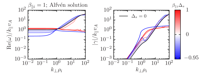
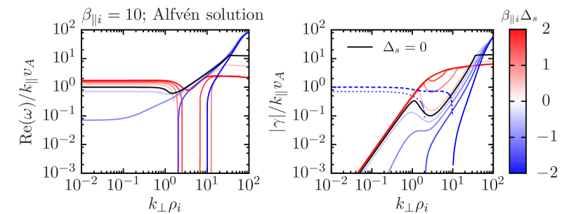
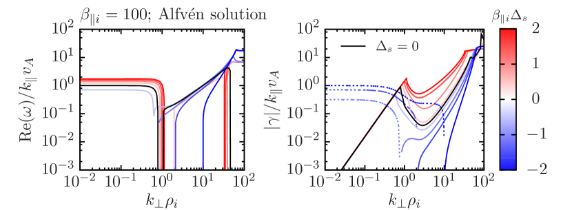
Figure 1: Real and imaginary parts of the frequency $\omega={\rm Re}(\omega)+{\rm i}\gamma$ on the Alfvénic branch as functions of $k_{\perp}\rho_{i}$ for $\beta_{\parallel i}=\beta_{\parallel e}=1$, $10$, and $100$. (Recall that $\rho_{i}\doteq v_{{\rm th}\perp i}/\Omega_{i}\propto\sqrt{\beta_{\perp i}}$, and so the abscissa is a function of pressure anisotropy.) Equal ion and electron equilibrium pressure anisotropies $\Delta_{s}$ are equally spaced from negative (blue) to positive (red) values, the hues of the lines darkening towards larger absolute values (as indicated by the color bars). The solution for a Maxwellian equilibrium, $\Delta_{s}=0$, is shown as the black line. Stable (unstable) modes are denoted by solid (dotted) lines. See §3.6.4 for discussion.

Figure 1 displays the real part, ${\rm Re}(\omega)$, and the absolute value of the imaginary part, $|\gamma|\doteq|{\rm Im}(\omega)|$, of the complex frequency $\omega$ (normalized to $k_{\parallel}v_{\rm A}$) describing waves on the Alfvénic branch as a function of $k_{\perp}\rho_{i}$, for varying $\beta_{\parallel i}$ and pressure anisotropy $\Delta_{i}$. We take $\beta_{\parallel e}=\beta_{\parallel i}$ and $\Delta_{e}=\Delta_{i}$ (i.e. $T_{\parallel 0{e}}=T_{\parallel 0{i}}$), so that the equal-temperature ions and electrons both contribute to the total pressure anisotropy of the equilibrium plasma. The solid black lines correspond to $\Delta_{s}=0$, i.e. to a Maxwellian equilibrium, and match those presented in figure 4 of Howes et al. (2006) and figure 8 of S09. The red (blue) lines correspond to positive (negative) equilibrium pressure anisotropy, their hues darkening towards larger absolute values (as indicated by the accompanying color bars).

For all values of $\beta_{\parallel i}$ and $\Delta_{s}$, the analytic solution (84) accurately describes the Alfvén waves (and the firehose-unstable modes) at long wavelengths, with negative (positive) pressure anisotropies decreasing (increasing) the effective Alfvén speed and, thus, the real part of the frequency. (Solutions for $\beta_{\parallel i}\ll 1$ are not presented, as very extreme pressure anisotropies are required to appreciably modify the waves in this case.) The weak damping affecting these pressure-anisotropy-modified Alfvén waves is obtained analytically in appendix B.1 for $\beta_{\parallel i}\gg 1$ with $k_{\perp}\rho_{i}\sim\mathcal{O}(\beta_{\parallel i}^{-1/4})$, $\overline{\omega}\sim\mathcal{O}(1)$ (see (178)):

$$\overline{\gamma}\simeq-\frac{9}{16}\frac{k^{2}_{\perp}\rho^{2}_{i}}{2}\sqrt{\frac{\beta_{\parallel i}}{\pi}},$$ (107)

which is independent (to leading order) of the pressure anisotropy (as it indeed is in the figure). For $\beta_{\parallel i}^{-1/4}\ll k_{\perp}\rho_{i}\ll 1$ (see (179a)), or $k_{\perp}\rho_{i}\sim\mathcal{O}(1)$, $\overline{\omega}\sim\mathcal{O}(\beta_{\parallel i}^{-1/2})$ (see (182b)), we have

$$\overline{\gamma}\simeq-\frac{8}{9}\biggl{(}1+\frac{\beta_{\parallel i}}{2}\Delta_{i}+\frac{\beta_{\parallel e}}{2}\Delta_{e}\biggr{)}\biggl{(}\frac{k^{2}_{\perp}\rho^{2}_{i}}{2}\biggr{)}^{-1}\sqrt{\frac{\pi}{\beta_{\parallel i}}}\frac{T_{\perp 0{i}}}{T_{\parallel 0{i}}},$$ (108)

which captures well the decrease of $|\overline{\gamma}|$ with $k_{\perp}\rho_{i}$ and its dependence on the pressure anisotropy that are seen in the $\beta_{\parallel i}=10$ and $100$ plots near $k_{\perp}\rho_{i}\sim 1$. For $k_{\perp}\rho_{i}\gg 1$, the damping rate increases again with $\alpha_{i}$ (see (B.1.2)), this time with an explicit dependence on the electron pressure anisotropy:

$$\overline{\gamma}\simeq-\frac{k^{2}_{\perp}\rho^{2}_{i}}{2}\sqrt{\frac{\pi}{\beta_{\parallel i}}}\biggl{(}1+\frac{\beta_{\parallel e}}{2}\Delta_{e}\biggr{)}\frac{T_{\perp 0{e}}^{2}}{T_{\parallel 0{e}}^{2}}\frac{T_{\parallel 0{i}}}{T_{\perp 0{i}}}\biggl{(}\frac{Z_{i}}{\tau_{\parallel{i}}}\frac{Z_{i}m_{e}}{m_{i}}\biggr{)}^{1/2}.$$ (109)

Positive anisotropy $\Delta_{e}>0$ increases the rate of collisionless damping by effectively increasing the Alfvén speed and thereby bringing the wave frequency (see (B.1.2)) closer to the ion-Landau resonance; this is manifest in the $\beta_{\parallel i}=10$ and $100$ panels of figure 1. Negative electron pressure anisotropy, on the other hand, drives these KAWs firehose unstable for $\Delta_{e}<-2/\beta_{\parallel e}$. Note that there exist Alfvénic fluctuations that are firehose unstable at long wavelengths, which become stable at short wavelengths (the blue lines that are absent at low $k_{\perp}$ but appear at high $k_{\perp}$ in the ${\rm Re}(\omega)$ panel). This is because the ion contribution to the total pressure anisotropy is only relevant at long wavelengths. Both the analytic solutions (cf. (84) and (93)) and the numerical solutions shown in figure 2 demonstrate this point.

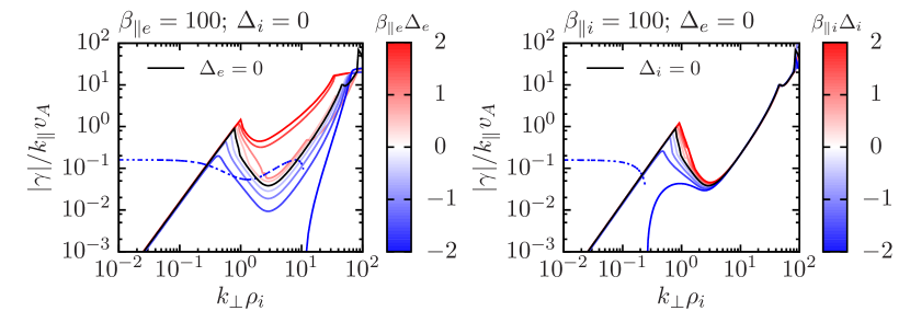
Figure 2: Imaginary part of the frequency $\omega={\rm Re}(\omega)+{\rm i}\gamma$ on the Alfvénic branch as a function of $k_{\perp}\rho_{i}$ for $\beta_{\parallel i}=\beta_{\parallel e}=100$. Either (left) the equilibrium ion distribution is taken to be isotropic, $\Delta_{i}=0$, or (right) the equilibrium electron distribution is taken to be isotropic, $\Delta_{e}=0$. Stable (unstable) modes are denoted by solid (dotted) lines. Sub-ion-Larmor fluctuations are primarily affected by electron pressure anisotropy, while long-wavelength fluctuations and the transition at $k_{\perp}\rho_{i}\sim 1$ are affected by both. See §3.6.4 for discussion.

In §3.6.2, we speculated that the location of the wavenumber transition from Alfvén waves to KAWs and the consequent ion-Larmor-scale spectral break that is routinely observed in kinetic turbulence (e.g. Leamon et al., 1998, 1999; Bale et al., 2005; Howes et al., 2006; Markovskii et al., 2008; Alexandrova et al., 2009; Chen et al., 2014) should be a function of the pressure anisotropy. This conjecture is supported especially by the $\beta_{\parallel i}=10$ and $100$ plots, which display a sharp frequency jump near $k_{\perp}\rho_{i}\sim 1$ at a location dependent upon the pressure anisotropy. This dependence can be estimated by equating the asymptotic damping rates (107) or (108) to the real frequency (84); this yields

$$(k_{\perp}\rho_{i})_{\rm break}\propto\biggl{(}1+\frac{\beta_{\parallel i}}{2}\Delta_{i}+\frac{\beta_{\parallel e}}{2}\Delta_{e}\biggr{)}^{1/4}.$$ (110)

Positive (negative) anisotropies are thus predicted to shift the ion-Larmor-scale spectral break towards larger (smaller) perpendicular wavenumbers. This frequency jump is seen to be accompanied by very strong ion Landau damping ($|\overline{\gamma}|\sim 1$), with order-of-magnitude variations in the damping rate depending upon $\Delta_{s}$. Note further that the width of the ${\rm Re}(\omega)=0$ gap at large $\beta_{\parallel i}$ near $k_{\perp}\rho_{i}\sim 1$, evident in the $\beta_{\parallel i}=100$ plot, increases with $\Delta_{s}>0$. (Figure 2 shows that both the ion and electron pressure anisotropies affect the strength of the collisionless damping and the location of the break point.)

Because the amount of Landau damping at these scales is likely to be related to how much energy ultimately goes into heating the ions or the electrons, pressure anisotropy ought to be considered alongside $\beta_{i}$ and $T_{0i}/T_{0e}$ when assessing the efficiency of ion heating. This consideration may be important for developing a quantitative and predictive theory of collisionless radiatively inefficient accretion flows, for which the efficiency of ion heating is a key unknown (e.g. Quataert & Gruzinov, 1999; Howes, 2010) and in which pressure anisotropy is predicted to govern much of the nonlinear dynamics and thermodynamics (e.g. Sharma et al., 2006, 2007; Kunz et al., 2016). We investigate this possibility quantitatively using a simple cascade model in §4.5. Here we simply examine which species (ions or electrons) contributes the most to the Landau damping of the Alfvénic fluctuations at different scales. In figure 3, the ratio of the absolute value of the imaginary part and the real part of the frequency, separated into contributions from damping on the ions (left panels) and on the electrons (right panels), are shown versus $k_{\perp}\rho_{i}$, $\beta_{\parallel i}$, and $\Delta_{s}$. (See §4.5 and, in particular, (167) for how this partitioning of $\gamma$ into $\gamma_{i}$ and $\gamma_{e}$ is computed.) In all cases, the collisionless damping on the ions is stronger than that on the electrons for $k_{\perp}\rho_{i}\lesssim 2$, whereas the collisionless damping on the electrons at sub-ion-Larmor scales is dominant. While the latter is much stronger than the former, one would anticipate in a turbulent cascade that the energy carried by the sub-ion-Larmor fluctuations would be much smaller than that carried by the long-wavelength Alfvénic fluctuations, and so the damping rates on both the ions and the electrons (and the impact of pressure anisotropy on them) are likely important for calculating ion versus electron heating (see §4.5).

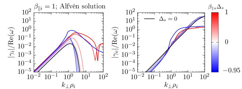
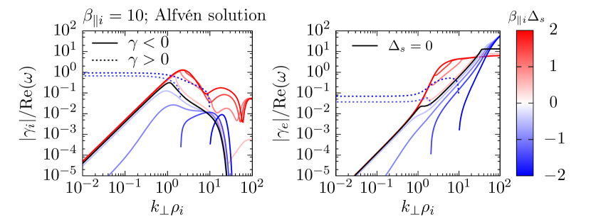
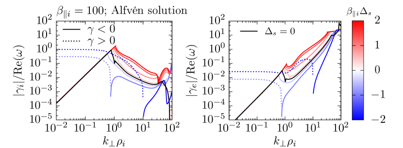
Figure 3: Ratio of damping/growth rate $|\gamma|$ and ${\rm Re}(\omega)$ on the Alfvénic branch, partitioned into contributions from damping on ions ($|\gamma_{i}|$; left panels) and electrons ($|\gamma_{e}|$; right panels), as a function of $k_{\perp}\rho_{i}$ for $\beta_{\parallel i}=\beta_{\parallel e}=1$, $10$, and $100$. Equal ion and electron equilibrium pressure anisotropies $\Delta_{s}$ are varied from negative (blue) to positive (red) values, with $\Delta_{s}=0$ indicated by the black line. Stable (unstable) modes are denoted by solid (dotted) lines. See §3.6.4 for discussion.

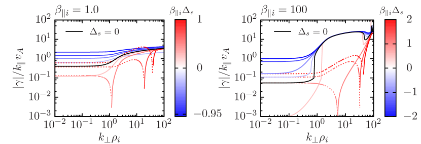
Figure 4: Imaginary part of the frequency $\omega={\rm Re}(\omega)+{\rm i}\gamma$ on the compressive branch as a function of $k_{\perp}\rho_{i}$ for $\beta_{\parallel i}=\beta_{\parallel e}=1$ and $100$. Equal ion and electron equilibrium pressure anisotropies $\Delta_{s}$ are varied from negative (blue) to positive (red) values, with $\Delta_{s}=0$ indicated by the black line. Stable (unstable) modes are denoted by solid (dotted) lines. See §3.6.4 for discussion.

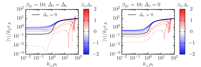
Figure 5: Imaginary part of the frequency $\omega={\rm Re}(\omega)+{\rm i}\gamma$ on the compressive branch as a function of $k_{\perp}\rho_{i}$ for $\beta_{\parallel i}=\beta_{\parallel e}=10$ and either (left) $\Delta_{i}=\Delta_{e}$ or (right) $\Delta_{i}=0$. Pressure anisotropies are varied from negative (blue) to positive (red) values, the hues of the lines darkening towards larger absolute values (as indicated by the color bars). The solution for a Maxwellian equilibrium, $\Delta_{s}=0$, is indicated by the black line. Stable (unstable) modes are denoted by solid (dotted) lines. Ion pressure anisotropy only affects the behaviour of the modes at long wavelengths, $k_{\perp}\rho_{i}\lesssim 1$. See §3.6.4 for discussion.

Figures 4 and 5 display the imaginary part of the frequency describing waves on the compressive branch as a function of $k_{\perp}\rho_{i}$, for varying plasma $\beta_{\parallel i}$ and pressure anisotropy $\Delta_{s}$. These modes always have ${\rm Re}(\omega)=0$ and thus are aperiodic. As in figure 1, the solid black lines correspond to $\Delta_{s}=0$, while the red (blue) lines correspond to positive (negative) equilibrium pressure anisotropy. In figure 4, we take $\beta_{\parallel e}=\beta_{\parallel i}$ and $\Delta_{e}=\Delta_{i}$, so that the equal-temperature ions and electrons both contribute to the total pressure anisotropy of the equilibrium plasma. By comparing solutions obtained using $\Delta_{i}=\Delta_{e}$ with those obtained using $\Delta_{i}=0$, figure 5 demonstrates that it is only the pressure anisotropy of the electrons that affects the sub-ion-Larmor range (as predicted in §3.6.3).

At long wavelengths ($k_{\perp}\rho_{i}\ll 1$), the damping/growth rate follows closely the “$+$” branch obtained from the dispersion relation (86), as it is the more weakly damped of the two branches. This is the branch that goes over to the aperiodic Barnes-damped/mirror-unstable slow mode for $\beta_{\perp s},\beta_{\parallel s}\gg 1$ (see (89)). As such, it is unstable if (91) is satisfied; the figures show this. At $k_{\perp}\rho\sim 1$, the character of the mode changes abruptly to become either strongly damped at a rate independent of the pressure anisotropy (see (106) for an approximation solution) or, if the pressure anisotropy is sufficiently positive, mirror-unstable at a rate given approximately by (93). Note that, in the latter case, the compressive solution is coupled to the Alfvénic solution, and the unstable mode is a KAW.

At electron-Larmor scales ($k_{\perp}\rho_{e}\gtrsim 1$), both branches of the dispersion relation – Alfvénic and compressive – are strongly damped via Landau resonance on the electrons.

This completes our discussion of the linear gyrokinetic theory. We now make use of the physics contained in these results to explain how pressure anisotropy affects the nonlinear turbulent cascade of free energy to small scales in phase space.

4 Generalised energy and the nonlinear kinetic cascade

4.1 KRMHD free-energy conservation for arbitrary $f_{0s}$

In Paper I, we showed that the long-wavelength Alfvénic and compressive fluctuations satisfy the following nonlinear conservation law:

$$\frac{{\rm d}W_{\rm KRMHD}}{{\rm d}t}=-\int{\rm d}^{3}\mbox{\boldmath{$r$}}\sum_{s}u^{\prime}_{\parallel 0s}\biggl{(}q_{s}\delta n_{s}E_{\parallel}-\delta p_{\perp s}\hat{\mbox{\boldmath{$b$}}}\,\mbox{\boldmath{$\cdot$}}\,\mbox{\boldmath{$\nabla$}}\frac{\delta B_{\parallel}}{B_{0}}\biggr{)},$$ (111)

where

$$W_{\rm KRMHD} \doteq\int{\rm d}^{3}\mbox{\boldmath{$r$}}\,\Biggl{\{}\sum_{s}\int{\rm d}^{3}\mbox{\boldmath{$v$}}\,\frac{T_{\parallel 0{s}}\delta\widetilde{f}^{2}_{s}}{2f^{\parallel}_{0s}}+\frac{\rho_{0}u^{2}_{\perp}}{2}$$

$$\quad+\Biggl{[}1+\sum_{s}\frac{\beta_{\parallel s}}{2}\Biggl{(}\Delta_{s}-\frac{2u^{\prime 2}_{\parallel 0s}}{v_{{\rm th}\parallel s}^{2}}\Biggr{)}\Biggr{]}\frac{\delta B^{2}_{\perp}}{8\pi}+\Biggl{(}1-\sum_{s}\beta_{\perp s}\Delta_{2s}\Biggr{)}\frac{\delta B_{\parallel}^{2}}{8\pi}\Biggr{\}}$$ (112)

is the generalised free energy of KRMHD,

$$\delta\widetilde{f}_{s}=\delta f_{s}(v_{\parallel},w_{\perp})+\frac{w^{2}_{\perp}}{v_{{\rm th}\perp s}^{2}}\frac{\delta B_{\parallel}}{B_{0}}\,\mathfrak{D}\!f_{0s}$$ (113)

is the (long-wavelength) perturbed distribution function in the frame of the Alfvénic fluctuations (see §I–4.2 and (50)), and $\Delta_{\ell s}\doteq\Delta_{\ell s}(0)$ (see (72)). (Recall from (44) that $\mbox{\boldmath{$w$}}_{\perp}\doteq\mbox{\boldmath{$v$}}-\mbox{\boldmath{$u$}}_{\perp}-\mbox{\boldmath{$v$}}\,\mbox{\boldmath{$\cdot$}}\,\hat{\mbox{\boldmath{$b$}}}\hat{\mbox{\boldmath{$b$}}}$ is the perpendicular component of the particle velocity peculiar to the $E$ $\times$ $B$ flow.) The parallel electric field $E_{\parallel}$ on the right-hand side of (111) is given by (I–2.37) – we have no need of restating its general form here; for a bi-Maxwellian equilibrium, it is given below by (129).

In the presence of mean interspecies drifts $u^{\prime}_{\parallel 0s}$, the right-hand side of (111) corresponds to the change in the free energy due to the minus work done by the fluctuating parallel electric and magnetic-mirror forces acting on the parallel-drifting particles. In the absence of these drifts, the right-hand side of (111) is zero. Then $W_{\rm KRMHD}$ is a quadratic invariant whose existence causes a turbulent cascade of generalised free energy in a pressure-anisotropic plasma to small scales in phase space across the inertial range. The invariant is comprised of three parts: two Alfvénic invariants $W^{+}_{\rm AW}$ and $W^{-}_{\rm AW}$ ((I–3.10), arising from the second and third terms in (4.1)) representing forward- and backward-propagating nonlinear Alfvén waves, and a compressive invariant $W_{\rm compr}$ ((I–4.7), arising from the first and fourth terms in (4.1)). In the pressure-isotropic case (eq. (201) of S09), the first term in (4.1) is the entropy of the perturbed distribution function. For a single-ion-species bi-Maxwellian equilibrium, the compressive invariant $W_{\rm compr}$ splits into three independently cascading parts: $W^{+}_{\rm compr}$, $W^{-}_{\rm compr}$, and $W_{\widetilde{g}_{i}}$, the latter of which represents a purely kinetic cascade. All three cascade channels lead to small perpendicular spatial scales via passive mixing by the Alfvénic turbulence and to small scales in $v_{\parallel}$ via the linear parallel phase mixing (§I–4.3 through §I–4.6; see however Schekochihin et al. (2016) for how nonlinear advection of the perturbed particle distribution by fluctuating flows might reduce the amount of parallel phase mixing). The rates of mixing are generally functions of the velocity-space anisotropy of the equilibrium function.

4.2 Gyrokinetic free-energy conservation for arbitrary $f_{0s}$

Our goal in this section is to derive the gyrokinetic generalisation of (111), valid at both long and short wavelengths and reducing to (111) in the former limit. The starting point is the gyrokinetic equation (47), written in terms of the gyrokinetic response $\widetilde{h}_{s}$. Multiplying that equation by $T_{\parallel 0{s}}\widetilde{h}_{s}/f^{\parallel}_{0s}$ and integrating over the velocities and gyrocentre positions, we find that the nonlinear term conserves the variance of $\widetilde{h}_{s}$ and so

$$\frac{{\rm d}}{{\rm d}t}\int{\rm d}^{3}\mbox{\boldmath{$v$}}\int{\rm d}^{3}\mbox{\boldmath{$R$}}_{s}\,\frac{T_{\parallel 0{s}}\widetilde{h}^{2}_{s}}{2f^{\parallel}_{0s}}=\int{\rm d}^{3}\mbox{\boldmath{$v$}}\int{\rm d}^{3}\mbox{\boldmath{$R$}}_{s}\,q_{s}\biggl{(}\frac{\partial\langle\chi\rangle_{\!\boldsymbol{R}_{s}}}{\partial t}+u^{\prime}_{\parallel 0s}\frac{\partial\langle\chi\rangle_{\!\boldsymbol{R}_{s}}}{\partial z}\biggr{)}\widetilde{h}_{s}.$$ (114)

We now sum this equation over all species. The right-hand side becomes

$$\sum_{s}q_{s} \int{\rm d}^{3}\mbox{\boldmath{$v$}}\int{\rm d}^{3}\mbox{\boldmath{$R$}}_{s}\,\biggl{(}\frac{\partial\langle\chi\rangle_{\!\boldsymbol{R}_{s}}}{\partial t}+u^{\prime}_{\parallel 0s}\frac{\partial\langle\chi\rangle_{\!\boldsymbol{R}_{s}}}{\partial z}\biggr{)}\widetilde{h}_{s}$$

$$=\int{\rm d}^{3}\mbox{\boldmath{$r$}}\sum_{s}q_{s}\int{\rm d}^{3}\mbox{\boldmath{$v$}}\,\biggl{\langle}\biggl{(}\frac{\partial\chi}{\partial t}+u^{\prime}_{\parallel 0s}\frac{\partial\chi}{\partial z}\biggr{)}\widetilde{h}_{s}\biggr{\rangle}_{{\negthickspace\!\boldsymbol{r}}}$$

$$=\int{\rm d}^{3}\mbox{\boldmath{$r$}}\,\Biggl{[}\frac{\partial\varphi}{\partial t}\sum_{s}q_{s}\int{\rm d}^{3}\mbox{\boldmath{$v$}}\,\langle\widetilde{h}_{s}\rangle_{\boldsymbol{r}}-\frac{1}{c}\frac{\partial\mbox{\boldmath{$A$}}}{\partial t}\,\mbox{\boldmath{$\cdot$}}\,\sum_{s}q_{s}\int{\rm d}^{3}\mbox{\boldmath{$v$}}\,\langle\mbox{\boldmath{$v$}}\widetilde{h}_{s}\rangle_{\boldsymbol{r}}$$

$$\qquad+\sum_{s}q_{s}u^{\prime}_{\parallel 0s}\int{\rm d}^{3}\mbox{\boldmath{$v$}}\,\biggl{\langle}\frac{\partial\chi}{\partial z}\,\widetilde{h}_{s}\biggr{\rangle}_{{\negthickspace\!\boldsymbol{r}}}\Biggr{]}.$$ (115)

The first term on the right-hand side of (4.2) can be written in terms of the potentials ($\varphi,A_{\parallel},\delta B_{\parallel}$) by using (46a) to unpack $\widetilde{h}_{s}$, employing the quasi-neutrality constraint (52), and performing the resulting integrals using the notation defined in appendix A. The second term on the right-hand side of (4.2) is most easily dealt with by using Faraday’s law (2) and Ampère’s law (4) to write

$$-\frac{{\rm d}}{{\rm d}t}\int{\rm d}^{3}\mbox{\boldmath{$r$}}\,\frac{|\delta\mbox{\boldmath{$B$}}|^{2}}{8\pi}=\int{\rm d}^{3}\mbox{\boldmath{$r$}}\,\mbox{\boldmath{$E$}}\,\mbox{\boldmath{$\cdot$}}\,\mbox{\boldmath{$j$}}=\int{\rm d}^{3}\mbox{\boldmath{$r$}}\,\Biggl{(}-\frac{1}{c}\frac{\partial\mbox{\boldmath{$A$}}}{\partial t}\,\mbox{\boldmath{$\cdot$}}\,\sum_{s}q_{s}\int{\rm d}^{3}\mbox{\boldmath{$v$}}\,\mbox{\boldmath{$v$}}\delta f_{s}\Biggr{)}$$

$$\quad=\int{\rm d}^{3}\mbox{\boldmath{$r$}}\,\Biggl{[}-\frac{1}{c}\frac{\partial\mbox{\boldmath{$A$}}}{\partial t}\,\mbox{\boldmath{$\cdot$}}\,\sum_{s}q_{s}\int{\rm d}^{3}\mbox{\boldmath{$v$}}\,\biggl{\langle}\mbox{\boldmath{$v$}}\biggl{(}\delta f_{1s,{\rm Boltz}}-\frac{q_{s}\langle\chi\rangle_{\!\boldsymbol{R}_{s}}}{T_{\perp 0{s}}}\,\mathfrak{D}\!f_{0s}+\widetilde{h}_{s}\biggr{)}\biggr{\rangle}_{{\negthickspace\!\boldsymbol{r}}}\Biggr{]}.$$ (116)

Then, substituting (25) for $\delta f_{1s,{\rm Boltz}}$ and performing the resulting integrals (again, with the aid of appendix A), we may use (4.2) to write the second term on the right-hand side of (4.2) in terms of the potentials ($\varphi,A_{\parallel},\delta B_{\parallel}$) and the rate of change of the magnetic energy. The third and final term on the right-hand side of (4.2) is markedly simplified by using (57) to move from $\widetilde{h}_{s}$ to $g_{s}$:

$$\int{\rm d}^{3}\mbox{\boldmath{$r$}}\sum_{s}q_{s}u^{\prime}_{\parallel 0s}\int{\rm d}^{3}\mbox{\boldmath{$v$}}\,\biggl{\langle}\frac{\partial\chi}{\partial z}\,\widetilde{h}_{s}\biggr{\rangle}_{{\negthickspace\!\boldsymbol{r}}}=\int{\rm d}^{3}\mbox{\boldmath{$r$}}\sum_{s}q_{s}u^{\prime}_{\parallel 0s}\int{\rm d}^{3}\mbox{\boldmath{$v$}}\,\biggl{\langle}\frac{\partial\chi}{\partial z}\,g_{s}\biggr{\rangle}_{{\negthickspace\!\boldsymbol{r}}}$$

$$\quad+\int{\rm d}^{3}\mbox{\boldmath{$r$}}\sum_{s}q_{s}u^{\prime}_{\parallel 0s}\int{\rm d}^{3}\mbox{\boldmath{$v$}}\,\frac{q_{s}f^{\parallel}_{0s}}{T_{\parallel 0{s}}}\Biggl{\langle}\frac{\partial\chi}{\partial z}\Biggl{\langle}\chi+\frac{(v_{\parallel}-u^{\prime}_{\parallel 0s})A_{\parallel}}{c}\Biggr{\rangle}_{{\negthickspace\!\boldsymbol{R}_{s}}}\Biggr{\rangle}_{{\negthickspace\!\boldsymbol{r}}},$$ (117)

from which we may remove the entire second line after integrating by parts with respect to $z$ (to eliminate the first term) and $v_{\parallel}$ (to eliminate the second).

Assembling (4.2)–(4.2) and cheerfully expending much algebraic effort, we find that (114) summed over species is equivalent to the following conservation law:

$$\frac{{\rm d}W_{\rm GK}}{{\rm d}t}=\int{\rm d}^{3}\mbox{\boldmath{$r$}}\sum_{s}u^{\prime}_{\parallel 0s}\int{\rm d}^{3}\mbox{\boldmath{$v$}}\,q_{s}g_{s}\Biggl{[}\bigl{\langle}\hat{\mbox{\boldmath{$b$}}}\bigr{\rangle}_{\!\boldsymbol{R}_{s}}\,\mbox{\boldmath{$\cdot$}}\,\mbox{\boldmath{$\nabla$}}\biggl{\langle}\varphi-\frac{\mbox{\boldmath{$v$}}_{\perp}\,\mbox{\boldmath{$\cdot$}}\,\mbox{\boldmath{$A$}}_{\perp}}{c}\biggr{\rangle}_{{\negthickspace\!\boldsymbol{R}_{s}}}+\frac{1}{c}\frac{\partial\langle A_{\parallel}\rangle_{\!\boldsymbol{R}_{s}}}{\partial t}\Biggr{]},$$ (118)

where

$$W_{\rm GK} \doteq\int{\rm d}^{3}\mbox{\boldmath{$r$}}\,\Biggl{\{}\sum_{s}\int{\rm d}^{3}\mbox{\boldmath{$v$}}\,\frac{T_{\parallel 0{s}}\delta\widetilde{f}^{2}_{s}}{2f^{\parallel}_{0s}}+\sum_{s}\frac{q^{2}_{s}n_{0s}}{2T_{\perp 0{s}}}\,\varphi\Bigl{(}C^{\perp}_{0s}-\widehat{\Gamma}^{\perp}_{00s}\Bigr{)}\varphi+\frac{\delta B^{2}_{\perp}}{8\pi}$$

$$\quad+\sum_{s}\frac{\beta_{\parallel s}}{2}\frac{A_{\parallel}}{\sqrt{4\pi}\rho_{s}}\Biggl{[}\frac{T_{\perp 0{s}}}{T_{\parallel 0{s}}}\Bigl{(}1-\widehat{\Gamma}_{00s}\Bigr{)}-\Bigl{(}C^{\perp}_{2s}-\widehat{\Gamma}^{\perp}_{02s}\Bigr{)}\Biggl{(}1+\frac{2u^{\prime 2}_{\parallel 0s}}{v_{{\rm th}\parallel s}^{2}}\Biggr{)}\Biggr{]}\frac{A_{\parallel}}{\sqrt{4\pi}\rho_{s}}$$

$$\quad+\frac{\delta B_{\parallel}}{\sqrt{8\pi}}\Biggl{[}1-\sum_{s}\beta_{\perp s}\Biggl{(}\frac{T_{\perp 0{s}}}{T_{\parallel 0{s}}}\frac{\widehat{\Gamma}^{\parallel}_{20s}}{2}-\frac{\widehat{\Gamma}^{\perp}_{20s}}{2}\Biggr{)}\Biggr{]}\frac{\delta B_{\parallel}}{\sqrt{8\pi}}-\sum_{s}q_{s}n_{0s}u^{\prime}_{\parallel 0s}\frac{A_{\parallel}}{c}\widehat{\Gamma}^{\perp}_{11s}\frac{\delta B_{\parallel}}{B_{0}}\Biggr{\}}$$ (119)

is the appropriately generalised gyrokinetic free energy. Here, $\delta\widetilde{f}_{s}$ is given by (50). The bi-linear differential operators in (4.2), conspicuously ornamented with the symbol $\,\widehat{\mbox{\,\,}}\,$, are defined in appendix A by (174). They result from integral combinations of various electromagnetic fields, gyro- and ring-averages of those fields, and various derivatives of the background distribution function: e.g.

$$\int{\rm d}^{3}\mbox{\boldmath{$r$}}\int{\rm d}^{3}\mbox{\boldmath{$v$}}\,\varphi\langle\langle\varphi\rangle_{\!\boldsymbol{R}_{s}}\rangle_{\boldsymbol{r}}\,f^{\perp}_{0s}\doteq n_{0s}\int{\rm d}^{3}\mbox{\boldmath{$r$}}\,\varphi\widehat{\Gamma}^{\perp}_{00s}\varphi\doteq n_{0s}\sum_{\boldsymbol{k}}\Gamma^{\perp}_{00s}(\alpha_{s})|\varphi_{\boldsymbol{k}}|^{2},$$

where the Fourier coefficient $\Gamma^{\perp}_{00}(\alpha_{s})$ is given by (171b). To leading order in $k^{2}_{\perp}\rho^{2}_{s}\ll 1$, the operators satisfy

$$\Psi\Bigl{(}C^{\perp}_{0s}-\widehat{\Gamma}^{\perp}_{00s}\Bigr{)}\Psi\approx\Psi\Bigl{(}1-\widehat{\Gamma}_{00s}\Bigr{)}\Psi\approx\Psi\Bigl{(}C^{\perp}_{2s}-\widehat{\Gamma}^{\perp}_{02s}\Bigr{)}\Psi\approx\sum_{\boldsymbol{k}}\alpha_{s}|\Psi_{\boldsymbol{k}}|^{2},$$

$$\widehat{\Gamma}^{\parallel}_{20s}\approx\frac{1}{n_{0s}}\int{\rm d}^{3}\mbox{\boldmath{$v$}}\,\frac{v^{4}_{\perp}}{v_{{\rm th}\perp s}^{4}}f^{\parallel}_{0s},\quad\widehat{\Gamma}^{\perp}_{20s}\approx 2,\quad\widehat{\Gamma}^{\perp}_{11s}\approx 1,$$ (120)

for any function $\Psi(\mbox{\boldmath{$r$}})$. Substituting these long-wavelength expressions into (4.2), eliminating its final term by using $\sum_{s}q_{s}n_{0s}u^{\prime}_{\parallel 0s}=0$, and manipulating (45) and (60) to write $\sum_{\boldsymbol{k}}k^{2}_{\perp}|\varphi_{\boldsymbol{k}}|^{2}$ and $\sum_{\boldsymbol{k}}k^{2}_{\perp}|A_{\parallel\boldsymbol{k}}|^{2}$ in terms of $u^{2}_{\perp}$ and $\delta B^{2}_{\perp}$, respectively, we find that the gyrokinetic invariant reduces to its KRMHD counterpart (4.1), as it should. More generally, equation (4.2) may be equivalently written in Fourier space using Parseval’s theorem as $W_{\rm GK}=\sum_{\boldsymbol{k}}W_{{\rm GK},\boldsymbol{k}}$, where

$$W_{{\rm GK},\boldsymbol{k}} =\sum_{s}\int{\rm d}^{3}\mbox{\boldmath{$v$}}\,\frac{T_{\parallel 0{s}}|\delta\widetilde{f}_{s\boldsymbol{k}}|^{2}}{2f^{\parallel}_{0s}}+\sum_{s}\frac{C^{\perp}_{0s}-\Gamma^{\perp}_{00s}(\alpha_{s})}{\alpha_{s}}\frac{m_{s}n_{0s}|\mbox{\boldmath{$u$}}_{\perp\boldsymbol{k}}|^{2}}{2}$$

$$+\Biggl{\{}1+\sum_{s}\frac{\beta_{\parallel s}}{2}\Biggl{[}\frac{T_{\perp 0{s}}}{T_{\parallel 0{s}}}\frac{1-\Gamma_{00s}(\alpha_{s})}{\alpha_{s}}-\frac{C^{\perp}_{2s}-\Gamma^{\perp}_{02s}(\alpha_{s})}{\alpha_{s}}\Biggl{(}1+\frac{2u^{\prime 2}_{\parallel 0s}}{v_{{\rm th}\parallel s}^{2}}\Biggr{)}\Biggr{]}\Biggr{\}}\frac{|\delta\mbox{\boldmath{$B$}}_{\perp\boldsymbol{k}}|^{2}}{8\pi}$$

$$+\Biggl{\{}1-\sum_{s}\beta_{\perp s}\Biggl{[}\frac{T_{\perp 0{s}}}{T_{\parallel 0{s}}}\frac{\Gamma^{\parallel}_{20s}(0,\alpha_{s})}{2}-\frac{\Gamma^{\perp}_{20s}(\alpha_{s})}{2}\Biggr{]}\Biggr{\}}\frac{|\delta B_{\parallel\boldsymbol{k}}|^{2}}{8\pi}$$

$$-\sum_{s}q_{s}n_{0s}u^{\prime}_{\parallel 0s}\Gamma^{\perp}_{11s}(\alpha_{s})\frac{A_{\parallel\boldsymbol{k}}^{\star}\delta B_{\parallel\boldsymbol{k}}}{cB_{0}},$$ (121)

where $\star$ denotes the complex conjugate.

Each of the terms in (4.2) (or (4.2)) deserves some discussion. The first term ($\propto$$\delta\widetilde{f}^{2}_{s}/f^{\parallel}_{0s}$) is due to the piece of the distribution function that represents changes in the kinetic energy of the particles due to interactions with the compressive fluctuations. In it are contributions from Landau-resonant particles, whose energy is changed by the parallel-electric and magnetic-mirror forces in such a way as to enable Landau (1946) and Barnes (1966) damping of compressive fluctuations. In the pressure-isotropic case, this term is simply the perturbed entropy of the system in the frame of the Alfvénic fluctuations (S09). The second term ($\propto$$\varphi^{2}$) represents the energy associated with the $E$ $\times$ $B$ motion. At long wavelengths, it is equal to $\rho_{0}u^{2}_{\perp}/2$ (see (45)). The next two terms represent the energetic cost of bending the magnetic-field lines (note that $k^{2}_{\perp}|A_{\parallel\boldsymbol{k}}|^{2}\propto|\delta\mbox{\boldmath{$B$}}_{\perp\boldsymbol{k}}|^{2}$), with an increase or decrease in this cost dependent upon the pressure anisotropy of the mean distribution function and the presence of interspecies drifts. The $\delta B_{\parallel}^{2}$ term signals a change in the energetic cost of compressing the magnetic-field lines ($\delta B_{\parallel}\neq 0$) because of background pressure anisotropy. The final term ($\propto$$A_{\parallel}\delta B_{\parallel}$) has no long-wavelength limit. It is related to conservation of helicity of the perturbed magnetic field,

$$\int{\rm d}^{3}\mbox{\boldmath{$r$}}\,\mbox{\boldmath{$A$}}\,\mbox{\boldmath{$\cdot$}}\,\delta\mbox{\boldmath{$B$}} =\int{\rm d}^{3}\mbox{\boldmath{$r$}}\,\bigl{[}\mbox{\boldmath{$A$}}_{\perp}\,\mbox{\boldmath{$\cdot$}}\,\bigl{(}\mbox{\boldmath{$\nabla$}}_{\perp}\,\mbox{\boldmath{$\times$}}\,A_{\parallel}\hat{\mbox{\boldmath{$z$}}}\bigr{)}+A_{\parallel}\delta B_{\parallel}\bigr{]}$$

$$=\int{\rm d}^{3}\mbox{\boldmath{$r$}}\,\bigl{[}A_{\parallel}\hat{\mbox{\boldmath{$z$}}}\,\mbox{\boldmath{$\cdot$}}\,\bigl{(}\mbox{\boldmath{$\nabla$}}_{\perp}\,\mbox{\boldmath{$\times$}}\,\mbox{\boldmath{$A$}}_{\perp}\bigr{)}+A_{\parallel}\delta B_{\parallel}\bigr{]}=2\int{\rm d}^{3}\mbox{\boldmath{$r$}}\,A_{\parallel}\delta B_{\parallel},$$ (122)

which is broken by parallel electric fields.

These parallel electric fields are on the right-hand side of (118), which is comprised of the fluctuating parallel force on gyrocentres multiplied by the number density of gyrocentres and the parallel interspecies drifts (recall that $g_{s}$ is the gyrocentre distribution function, (57)). In the long-wavelength limit, the right-hand side of (118) is precisely the same as the right-hand side of (4.2) – the work done on the plasma by the fluctuating parallel-electric and magnetic-mirror forces acting on the equilibrium drifts. The only difference in the gyrokinetic limit is that these (ring-averaged) parallel forces effectively act on the guiding centres instead of on the particles.

As explained in Paper I, because we have ordered collisions out of our equations, the long-wavelength invariant given by (4.1) is just one of an infinite number of invariants of the system. The same holds true for the more general invariant $W_{\rm GK}$ (4.2) derived here. The invariant $W_{\rm GK}$ does, however, have special significance for (at least) two reasons.

First, $W_{\rm GK}$ properly reduces to the gyrokinetic free-energy invariant for a (collisional) Maxwellian plasma (cf. (74) of S09):

$$W_{\rm GK} \rightarrow\int{\rm d}^{3}\mbox{\boldmath{$r$}}\,\Biggl{[}\sum_{s}\int{\rm d}^{3}\mbox{\boldmath{$v$}}\,\frac{T_{0s}\delta\widetilde{f}^{2}_{s}}{2f_{0s}}+\sum_{s}\frac{q^{2}_{s}n_{0s}}{2T_{0s}}\,\varphi\Bigl{(}1-\widehat{\Gamma}_{00s}\Bigr{)}\varphi+\frac{|\delta\mbox{\boldmath{$B$}}|^{2}}{8\pi}\Biggr{]},$$ (123a)

$$=\int{\rm d}^{3}\mbox{\boldmath{$r$}}\,\Biggl{(}\sum_{s}\int{\rm d}^{3}\mbox{\boldmath{$v$}}\,\frac{T_{0s}\delta f^{2}_{s}}{2f_{0s}}+\frac{|\delta\mbox{\boldmath{$B$}}|^{2}}{8\pi}\Biggr{)},$$ (123b)

which is the gyrokinetic version of a kinetic invariant variously referred to as the generalised grand canonical potential (Hallatschek, 2004) or free energy (Fowler, 1968; Brizard, 1994; Scott, 2010) because of its similarity to the Helmholtz free energy. It is the only quadratic invariant of Maxwellian gyrokinetics in three dimensions (S09).

Secondly, $W_{\rm GK}$ affords a thermodynamic interpretation of the effect of the mirror and firehose (in)stability parameters on nonlinear fluctuations. When the plasma is linearly stable, $W_{\rm GK}$ is a positive-definite quantity that measures the amount of (generalised) free energy carried by the fluctuations. As the stability thresholds are approached, it becomes energetically ‘cheaper’ to bend ($\delta\mbox{\boldmath{$B$}}_{\perp}$) or compress/rarefy ($\delta B_{\parallel}$) the magnetic-field lines, depending upon the sign of the pressure anisotropy; negative anisotropy effectively weakens the restoring magnetic-tension force, while positive anisotropy reduces the magnetic pressure response. When the plasma is unstable, $W_{\rm GK}$ is minimised by growing fluctuations. See §I–3.3 and §I–4.1 and for further discussion.

With a general invariant $W_{\rm GK}$ (4.2) in hand, valid across all scales (as long as they satisfy the gyrokinetic ordering), we now ask how the phase-space cascade begun in the inertial range (i.e. $k_{\perp}\rho_{i}\ll 1$) proceeds through the sub-ion-Larmor kinetic range (i.e. $k_{\perp}\rho_{i}\gg 1$). In the next section, we show that the power arriving from the inertial range is redistributed at $k_{\perp}\rho_{i}\sim 1$ into two independent cascades: a KAW cascade and an ion-entropy cascade. Just how this power is redistributed is a function of the background pressure anisotropy, the plasma beta parameter, the ion-to-electron temperature ratio, and, in particular, the background interspecies drifts, which are responsible for the source term on the right-hand side of (118). This source term represents the work done by fluctuations as they extract free energy from these flows, a process that requires the electric and magnetic-mirror forces involved to be coherent on time scales long enough to affect said flows (which are taken to be $\sim$$v_{{\rm th}\parallel i}$). For $k_{\perp}\rho_{i}\gg 1$, the fluctuations have frequencies too large and amplitudes too small for this source term to matter, and $W_{\rm GK}$ is approximately conserved. In fact, for $\beta_{\perp s}\sim\beta_{\parallel s}\sim 1$, all terms proportional to $u^{\prime}_{\parallel 0s}$ vanish to leading order in $k_{\perp}\rho_{i}$ from the dynamical equations, and the KAW and ion-entropy cascades proceed independently, without regard for the presence of background interspecies drifts. For that reason, we keep the following exposition as simple as possible by focusing exclusively on the single-ion-species, bi-Maxwellian case. Nothing of great import appears to be gainable by carrying around sums over ion species and various $C^{\parallel}_{\ell s}$ and $C^{\perp}_{\ell s}$ coefficients.

4.3 Gyrokinetic free energy in the sub-ion-Larmor range

In the wavenumber range $k_{\perp}\rho_{e}\ll 1\ll k_{\perp}\rho_{i}$, the $\widehat{\Gamma}_{\ell m}$ operators in the gyrokinetic free energy (4.2) take on the long-wavelength limits (4.2) for the electrons and vanish to leading order for the ions. Equation (4.2) then becomes

$$W_{\rm GK} \rightarrow\int{\rm d}^{3}\mbox{\boldmath{$r$}}\,\Biggl{\{}\int{\rm d}^{3}\mbox{\boldmath{$v$}}\,\frac{T_{\parallel 0{i}}\widetilde{h}^{2}_{i}}{2f_{0i}}+\int{\rm d}^{3}\mbox{\boldmath{$v$}}\,\frac{T_{\parallel 0{e}}\delta\widetilde{f}^{2}_{e}}{2f_{0e}}+\frac{p_{\perp 0i}}{2}\biggl{(}\frac{Z_{i}e\varphi}{T_{\perp 0{i}}}\biggr{)}^{2}$$

$$\quad+\biggl{(}1+\frac{\beta_{\parallel e}}{2}\Delta_{e}\biggr{)}\frac{\delta B^{2}_{\perp}}{8\pi}+\bigl{(}1-\beta_{\perp e}\Delta_{e}\bigr{)}\frac{\delta B_{\parallel}^{2}}{8\pi}\Biggr{\}}.$$ (124)

To simplify this expression further, we employ the mass-ratio expansion implicit in the $k_{\perp}\rho_{e}\ll 1\ll k_{\perp}\rho_{i}$ ordering to obtain the leading-order electron kinetic response (see (I–C73))

$$\delta\widetilde{f}_{e}=g_{e}+\frac{v^{2}_{\perp}}{v_{{\rm th}\parallel e}^{2}}\frac{\delta B_{\parallel}}{B_{0}}f^{\parallel}_{0e}=\biggl{(}\frac{\delta n_{e}}{n_{0e}}+\Delta_{e}\frac{\delta B_{\parallel}}{B_{0}}\biggr{)}f_{0e},$$ (125)

as well as the reduced quasi-neutrality constraint $\delta n_{e}/n_{0e}=-Z_{i}e\varphi/T_{\perp 0{i}}$ (see (95a)). Substituting these approximations into (4.3) gives

$$W_{\rm GK} \rightarrow\int{\rm d}^{3}\mbox{\boldmath{$r$}}\,\Biggl{\{}\int{\rm d}^{3}\mbox{\boldmath{$v$}}\,\frac{T_{\parallel 0{i}}\widetilde{h}^{2}_{i}}{2f_{0i}}+\frac{p_{\parallel 0e}}{2}\biggl{(}-\frac{Z_{i}e\varphi}{T_{\perp 0{i}}}+\Delta_{e}\frac{\delta B_{\parallel}}{B_{0}}\biggr{)}^{2}+\frac{p_{\perp 0i}}{2}\biggl{(}\frac{Z_{i}e\varphi}{T_{\perp 0{i}}}\biggr{)}^{2}$$

$$\quad+\biggl{(}1+\frac{\beta_{\parallel e}}{2}\Delta_{e}\biggr{)}\frac{\delta B^{2}_{\perp}}{8\pi}+\bigl{(}1-\beta_{\perp e}\Delta_{e}\bigr{)}\frac{\delta B_{\parallel}^{2}}{8\pi}\Biggr{\}}$$ (126)

$$\doteq W_{\widetilde{h}_{i}}+W_{\rm KAW}.$$ (127)

The first term, $W_{\widetilde{h}_{i}}$, is proportional to the total variance of $\widetilde{h}_{i}$; its cascade to small scales in phase space is discussed in §4.3.2. The remaining terms in (126) constitute the independently cascaded KAW energy $W_{\rm KAW}$. We shall show in the next two subsections that these two parts, $W_{\widetilde{h}_{i}}$ and $W_{\rm KAW}$, are independently conserved. How the total generalised gyrokinetic free energy $W_{\rm GK}$ is partitioned between them is determined at $k_{\perp}\rho_{i}\sim 1$, which ultimately sets the amount of ion versus electron heating.

4.3.1 ERMHD and the KAW cascade

Using (95d) to relate the magnetic-field-strength fluctuation $\delta B_{\parallel}$ in the sub-ion-Larmor range to the electrostatic potential $\varphi$, writing the energy in the perpendicular magnetic field $\delta B^{2}_{\perp}$ as $|\mbox{\boldmath{$\nabla$}}_{\perp}A_{\parallel}|^{2}$, and re-introducing the stream and flux functions via (96), the KAW invariant that appears in (127) may be written as

$$W_{\rm KAW} =\int{\rm d}^{3}\mbox{\boldmath{$r$}}\,\frac{m_{i}n_{0i}}{2}\biggl{\{}\biggl{(}1+\frac{\beta_{\parallel e}}{2}\Delta_{e}\biggr{)}|\mbox{\boldmath{$\nabla$}}_{\perp}\Psi|^{2}$$

$$+\frac{1-\beta_{\perp e}\Delta_{e}+\mathcal{K}}{(1-\beta_{\perp e}\Delta_{e}/2)^{2}}\biggl{(}1+\frac{Z_{i}T_{\parallel 0{e}}}{T_{\perp 0{i}}}\biggr{)}\biggl{[}2+\beta_{\perp i}\biggl{(}1+\frac{Z_{i}T_{\parallel 0{e}}}{T_{\perp 0{i}}}\biggr{)}-\beta_{\parallel e}\Delta^{2}_{e}\biggr{]}\frac{\Phi^{2}}{\rho^{2}_{i}}\biggr{\}}$$ (128a)

$$=\int{\rm d}^{3}\mbox{\boldmath{$r$}}\,\frac{m_{i}n_{0i}}{4}\bigl{(}\,|\Theta^{+}|^{2}+|\Theta^{-}|^{2}\,\bigr{)},$$ (128b)

which is the sum of the energies of the “$+$” and “$-$” linear KAW eigenmodes found in equation (3.6.2). This decomposition of the KAW invariant into a sum of energies of the $\Theta^{+}$ and $\Theta^{-}$ fluctuations underlies the scaling theory of KAW turbulence presented in S09. That theory is based on the reasoning (i) that $\Theta^{+}$ and $\Theta^{-}$ are nonlinearly coupled and thus should have similar scaling with $k_{\perp}$, (ii) that they obey a constant-flux cascade to small spatial scales through local interactions, and (iii) that critical balance holds for the KAW fluctuations. As long as the plasma remains mirror- and firehose-stable, the resulting scaling laws are not expected to change (although the overall fluctuation amplitudes will; see §4.4).

We now show that the form of $W_{\rm KAW}$ in (128) can be similarly obtained from the equations describing nonlinear KAWs – so-called electron reduced magnetohydrodynamics (ERMHD) – and thus is the “fluid energy” conserved during the nonlinear cascade of KAWs to small spatial scales.

In appendix C.8 of Paper I, we derived, via a mass-ratio expansion, nonlinear equations describing the electron kinetics for $k_{\perp}\rho_{e}\sim k_{\perp}\rho_{i}(m_{e}/m_{i})^{1/2}\ll 1$. For the purposes of the present paper, the two most important electron equations are those specifying the parallel electric field (see (I–C72))

$$E_{\parallel}=-\hat{\mbox{\boldmath{$b$}}}\,\mbox{\boldmath{$\cdot$}}\,\mbox{\boldmath{$\nabla$}}\varphi-\frac{1}{c}\frac{\partial A_{\parallel}}{\partial t}=-\hat{\mbox{\boldmath{$b$}}}\,\mbox{\boldmath{$\cdot$}}\,\mbox{\boldmath{$\nabla$}}\frac{T_{\parallel 0{e}}}{e}\biggl{(}\frac{\delta n_{e}}{n_{0e}}+\Delta_{e}\frac{\delta B_{\parallel}}{B_{0}}\biggr{)}$$ (129)

and what amounts to a reduced electron continuity equation (see (I–C78) and the accompanying discussion in §I–C.8.3):

$$\frac{{\rm d}}{{\rm d}t}\biggl{(}\frac{\delta n_{e}}{n_{0e}}-\frac{\delta B_{\parallel}}{B_{0}}\biggr{)}+\hat{\mbox{\boldmath{$b$}}}\,\mbox{\boldmath{$\cdot$}}\,\mbox{\boldmath{$\nabla$}}u^{(1)}_{\parallel e}+\frac{cT_{\perp 0{e}}}{eB_{0}}\biggl{\{}\frac{\delta n_{e}}{n_{0e}},\frac{\delta B_{\parallel}}{B_{0}}\biggr{\}}=0,$$ (130)

where

$$\frac{{\rm d}}{{\rm d}t}\doteq\frac{\partial}{\partial t}+\mbox{\boldmath{$u$}}_{\perp}\,\mbox{\boldmath{$\cdot$}}\,\mbox{\boldmath{$\nabla$}}=\frac{\partial}{\partial t}+\frac{c}{B_{0}}\bigl{\{}\varphi,\dots\bigr{\}}$$ (131)

is the Lagrangian time derivative measured in a frame transported at the $E$ $\times$ $B$ drift velocity, $\mbox{\boldmath{$u$}}_{\perp}$ (defined by (45)), and

$$u^{(1)}_{\parallel e}\doteq\frac{1}{n_{0e}}\int{\rm d}^{3}\mbox{\boldmath{$v$}}\,v_{\parallel}g^{(1)}_{e}=\frac{c}{4\pi en_{0e}}\biggl{(}1+\frac{\beta_{\parallel e}}{2}\Delta_{e}\biggr{)}\nabla^{2}_{\perp}A_{\parallel}$$ (132)

is the parallel electron flow velocity associated with the $\mathcal{O}(\sqrt{m_{e}/m_{i}})$ piece of $g_{e}$, denoted $g^{(1)}_{e}$ in Paper I (see §I–C.8).

Using (95a) and (95d) for the electron density fluctuation and the magnetic-field-strength fluctuation in the sub-ion-Larmor scale range, and introducing $\Phi$ and $\Psi$ via (96), we find that equations (129) and (130) become, respectively,

$$\frac{\partial\Psi}{\partial t}=v_{\rm A}\Biggl{\{}1+\frac{Z_{i}T_{\parallel 0{e}}}{T_{\perp 0{i}}}\Biggl{[}1-\frac{\beta_{\perp e}}{2}\Delta_{e}\biggl{(}\frac{1+\tau_{\perp{i}}/Z_{i}}{1-\beta_{\perp e}\Delta_{e}/2}\biggr{)}\Biggr{]}\Biggr{\}}\hat{\mbox{\boldmath{$b$}}}\,\mbox{\boldmath{$\cdot$}}\,\mbox{\boldmath{$\nabla$}}\Phi,$$ (133)

$$\frac{\partial\Phi}{\partial t}\Biggl{[}2+\beta_{\perp i}\biggl{(}\frac{1+Z_{i}/\tau_{\perp{i}}}{1-\beta_{\perp e}\Delta_{e}/2}\biggr{)}\Biggr{]}=-v_{\rm A}\biggl{(}1+\frac{\beta_{\parallel e}}{2}\Delta_{e}\biggr{)}\hat{\mbox{\boldmath{$b$}}}\,\mbox{\boldmath{$\cdot$}}\,\mbox{\boldmath{$\nabla$}}\rho^{2}_{i}\nabla^{2}_{\perp}\Psi.$$ (134)

These equations generalize the linear theory of KAWs (§3.6.2) to the nonlinear regime (cf. equations (226)–(227) of S09, to which (133)–(134) reduce in the pressure-isotropic limit). Introducing the perturbed magnetic-field vector

$$\frac{\delta\mbox{\boldmath{$B$}}}{B_{0}}=\frac{1}{v_{\rm A}}\hat{\mbox{\boldmath{$z$}}}\,\mbox{\boldmath{$\times$}}\,\mbox{\boldmath{$\nabla$}}_{\perp}\Psi+\hat{\mbox{\boldmath{$z$}}}\frac{\delta B_{\parallel}}{B_{0}}$$ (135)

with $\delta B_{\parallel}$ given by (95d), equations (133) and (134) can be recast as two coupled evolution equations for the perpendicular and parallel components of the perturbed magnetic field, respectively.

We now show that (133) and (134) conserve the energy $W_{\rm KAW}$ given by (128). First, apply $\mbox{\boldmath{$\nabla$}}_{\perp}$ to (133) and dot the result with $(1+\beta_{\parallel e}\Delta_{e}/2)\mbox{\boldmath{$\nabla$}}_{\perp}\Psi$; then integrate over space and use integration by parts to obtain

$$\frac{{\rm d}}{{\rm d}t}\int{\rm d}^{3}\mbox{\boldmath{$r$}}\,\frac{1}{2}\biggl{(}1+\frac{\beta_{\parallel e}}{2}\Delta_{e}\biggr{)}|\mbox{\boldmath{$\nabla$}}_{\perp}\Psi|^{2}=-\int{\rm d}^{3}\mbox{\boldmath{$r$}}\,v_{\rm A}\biggl{(}1+\frac{\beta_{\parallel e}}{2}\Delta_{e}\biggr{)}$$

$$\quad\times\Biggl{\{}1+\frac{Z_{i}T_{\parallel 0{e}}}{T_{\perp 0{i}}}\Biggl{[}1-\frac{\beta_{\perp e}}{2}\Delta_{e}\biggl{(}\frac{1+\tau_{\perp{i}}/Z_{i}}{1-\beta_{\perp e}\Delta_{e}/2}\biggr{)}\Biggr{]}\Biggr{\}}\bigl{(}\nabla^{2}_{\perp}\Psi\bigr{)}\hat{\mbox{\boldmath{$b$}}}\,\mbox{\boldmath{$\cdot$}}\,\mbox{\boldmath{$\nabla$}}\Phi.$$ (136)

Next, we multiply (134) by $(1+Z_{i}T_{\parallel 0{e}}/T_{\perp 0{i}})(1-\beta_{\perp e}\Delta_{e}/2)(\Phi/\rho^{2}_{i})$, integrate over space, and use integration by parts to find

$$\frac{{\rm d}}{{\rm d}t}\int{\rm d}^{3}\mbox{\boldmath{$r$}}\,\frac{1}{2}\biggl{(}1+\frac{Z_{i}T_{\parallel 0{e}}}{T_{\perp 0{i}}}\biggr{)}\biggl{[}2+\beta_{\perp i}\biggl{(}1+\frac{Z_{i}T_{\parallel 0{e}}}{T_{\perp 0{i}}}\biggr{)}-\beta_{\parallel e}\Delta^{2}_{e}\biggr{]}\frac{\Phi^{2}}{\rho^{2}_{i}}$$

$$\quad=\int{\rm d}^{3}\mbox{\boldmath{$r$}}\,v_{\rm A}\biggl{(}1+\frac{\beta_{\parallel e}}{2}\Delta_{e}\biggr{)}\biggl{(}1+\frac{Z_{i}T_{\parallel 0{e}}}{T_{\perp 0{i}}}\biggr{)}\biggl{(}1-\frac{\beta_{\perp e}}{2}\Delta_{e}\biggr{)}(\hat{\mbox{\boldmath{$b$}}}\,\mbox{\boldmath{$\cdot$}}\,\mbox{\boldmath{$\nabla$}}\Phi)\nabla^{2}_{\perp}\Psi.$$ (137)

Further multiplying (4.3.1) by a factor of $(1-\beta_{\perp e}\Delta_{e}+\mathcal{K})/(1-\beta_{\perp e}\Delta_{e}/2)^{2}$ and adding it to (4.3.1) cancels their right-hand sides and gives

$$\frac{{\rm d}W_{\rm KAW}}{{\rm d}t}=0,$$ (138)

with the KAW invariant $W_{\rm KAW}$ identical to that given by (128).

It is clear from the ERMHD equations (133) and (134), as well as from the form of the quadratic quantity they conserve (128), that electron pressure anisotropy influences the ability of the plasma to support certain magnetic-field perturbations. As the firehose threshold is approached from the stable side (i.e. $1+\beta_{\parallel e}\Delta_{e}/2\rightarrow 0^{+}$), the energetic cost for a KAW to bend the magnetic-field lines is reduced. Likewise, as the mirror threshold is approached from the stable side (i.e. $1-\beta_{\perp e}\Delta_{e}+\mathcal{K}\rightarrow 0^{+}$), the energetic cost for a KAW to compress/rarefy the magnetic-field lines is reduced. Beyond these thresholds, it becomes energetically profitable to grow these fluctuations. (Again, note that these instabilities themselves fall outside of the gyrokinetic ordering employed here.) Equation (138) thus establishes a thermodynamic connection between the linear and nonlinear stability of KAWs.

Before proceeding to investigate the ion-entropy cascade, in which $W_{\widetilde{h}_{i}}$ is independently conserved, we briefly remark on the case of $\Delta_{e}=2/\beta_{\perp e}$, for which the nonlinear ERMHD equations (133) and (134) are ill-posed. Instead, the appropriate nonlinear equations are

$$\frac{1}{v_{A}d_{i}}\frac{\partial A_{\parallel}}{\partial t}=\frac{\beta_{\parallel e}}{2}\Delta_{e}\,\hat{\mbox{\boldmath{$b$}}}\,\mbox{\boldmath{$\cdot$}}\,\mbox{\boldmath{$\nabla$}}\delta B_{\parallel}=\frac{1}{1+2/\beta_{\perp e}}\,\hat{\mbox{\boldmath{$b$}}}\,\mbox{\boldmath{$\cdot$}}\,\mbox{\boldmath{$\nabla$}}\delta B_{\parallel},$$ (139)

$$\frac{1}{v_{A}d_{i}}\frac{\partial\delta B_{\parallel}}{\partial t}=\biggl{(}1+\frac{\beta_{\parallel e}}{2}\Delta_{e}\biggr{)}\hat{\mbox{\boldmath{$b$}}}\,\mbox{\boldmath{$\cdot$}}\,\mbox{\boldmath{$\nabla$}}\nabla^{2}_{\perp}A_{\parallel}=\frac{2+2/\beta_{\perp e}}{1+2/\beta_{\perp e}}\,\hat{\mbox{\boldmath{$b$}}}\,\mbox{\boldmath{$\cdot$}}\,\mbox{\boldmath{$\nabla$}}\nabla^{2}_{\perp}A_{\parallel},$$ (140)

which of course return the eigenvectors (100) and growth/decay rates (101) in the linear regime. The corresponding conserved energy is

$$W_{\rm KAW}=\int{\rm d}^{3}\mbox{\boldmath{$r$}}\,\Biggl{[}\biggl{(}2+\frac{2}{\beta_{\perp e}}\biggr{)}\frac{\delta B^{2}_{\perp}}{8\pi}-\frac{\delta B_{\parallel}^{2}}{8\pi}\Biggr{]}\biggl{(}1+\frac{2}{\beta_{\perp e}}\biggr{)}^{-1},$$ (141)

which, as with (128), may be written as the sum of the energies of the “$+$” and “$-$” linear KAW eigenmodes found in equation (100). Note that, if $\delta B_{\parallel}^{2}$ grows or decays, so too must $\delta B^{2}_{\perp}$ grow or decay proportionally to keep $W_{\rm KAW}$ constant. As explained after (101), the resulting instability occurs because perpendicular pressure balance is maintained for any $\delta B_{\parallel}$ so long as $\Delta_{e}=2/\beta_{\perp e}$.

4.3.2 Ion-entropy cascade

The other piece of the gyrokinetic invariant, $W_{\widetilde{h}_{i}}$ (see (127)), represents the cascade of ion-entropy fluctuations to small scales in phase space (velocity and position) via nonlinear phase mixing in the gyrocentre space (see §7.9 of S09 for further details). It may be obtained directly from the gyrokinetic equation (47) as follows.

In the sub-ion-Larmor range, the ring-averaged gyrokinetic potential $\langle\chi\rangle_{\!\boldsymbol{R}_{i}}$ is dominated by the contribution from the electrostatic potential:

$$\frac{Z_{i}e}{T_{\perp 0{i}}}\langle\chi_{\boldsymbol{k}}\rangle_{\!\boldsymbol{R}_{i}} =\frac{2}{\sqrt{\beta_{\perp i}}}\biggl{\{}\biggl{[}J_{0}(a_{i})+\frac{v^{2}_{\perp}}{v^{2}_{\rm A}}\frac{J_{1}(a_{i})}{a_{i}}\frac{1+Z_{i}/\tau_{\perp{i}}}{1-\beta_{\perp e}\Delta_{e}/2}\biggr{]}\frac{\Phi_{\boldsymbol{k}}}{\rho_{i}v_{\rm A}}+J_{0}(a_{i})\frac{v_{\parallel}}{v_{\rm A}}\frac{\Psi_{\boldsymbol{k}}}{\rho_{i}v_{\rm A}}\biggr{\}}$$

$$\simeq\frac{2}{\sqrt{\beta_{\perp i}}}\sqrt{\frac{2}{\pi a_{i}}}\cos\Bigl{(}a_{i}-\frac{\pi}{4}\Bigr{)}\frac{\Phi_{\boldsymbol{k}}}{\rho_{i}v_{\rm A}}\quad{\rm for}~{}a_{i}\doteq k_{\perp}\rho_{i}\frac{v_{\perp}}{v_{{\rm th}\perp i}}\gg 1,$$ (142)

because of the KAW scaling $\Psi_{\boldsymbol{k}}\sim\Phi_{\boldsymbol{k}}/k_{\perp}\rho_{i}$ (see (3.6.2)). The gyrokinetic equation (47) in the sub-ion-Larmor range is then

$$\frac{\partial\widetilde{h}_{i}}{\partial t}+v_{\parallel}\frac{\partial\widetilde{h}_{i}}{\partial z}+\{\langle\Phi\rangle_{\!\boldsymbol{R}_{i}},\widetilde{h}_{i}\}=\frac{Z_{i}eB_{0}}{cT_{\parallel 0{i}}}\frac{\partial\langle\Phi\rangle_{\!\boldsymbol{R}_{i}}}{\partial t}f_{0i}.$$ (143)

This equation states that $\widetilde{h}_{i}$ is linearly phase-mixed by parallel-streaming ions, nonlinearly phase-mixed in the gyrocentre space by ring-averaged $E$ $\times$ $B$ flows (i.e. KAW turbulence), and sourced by wave-particle interactions, which become asymptotically small as $k_{\perp}\rho_{i}\gg 1$. Multiplying (143) by $T_{\parallel 0{i}}\widetilde{h}_{i}/f_{0i}$ and integrating over the phase space, we obtain

$$\frac{{\rm d}W_{\widetilde{h}_{i}}}{{\rm d}t}\doteq\frac{{\rm d}}{{\rm d}t}\int{\rm d}^{3}\mbox{\boldmath{$v$}}\int{\rm d}^{3}\mbox{\boldmath{$R$}}_{i}\,\frac{T_{\parallel 0{i}}\widetilde{h}^{2}_{i}}{2f_{0i}}=\frac{Z_{i}eB_{0}}{c}\int{\rm d}^{3}\mbox{\boldmath{$v$}}\int{\rm d}^{3}\mbox{\boldmath{$R$}}_{i}\,\frac{\partial\langle\Phi\rangle_{\!\boldsymbol{R}_{i}}}{\partial t}\widetilde{h}_{i}.$$ (144)

Deep in the sub-ion-Larmor range, the right-hand side of (144) representing the collisionless damping at the ion gyroscale is small and the total variance of $\widetilde{h}_{i}$ is conserved (as was shown also by equation (127)). The ion-entropy fluctuations are transferred across this scale range by means of a cascade, in which particles with like gyrocentre positions but with different $v_{\perp}$ (and so different gyroradii) sample spatially decorrelated electromagnetic fluctuations and thus $\hat{\mbox{\boldmath{$z$}}}\,\mbox{\boldmath{$\times$}}\,\mbox{\boldmath{$\nabla$}}\langle\Phi\rangle_{\!\boldsymbol{R}_{i}}$ drift with different velocities.

Equation (144) makes clear that neither ion nor electron pressure anisotropy (in a bi-Maxwellian plasma) affects the ion-entropy cascade itself. Instead, by shifting the precise $k$-space location of the frequency break that occurs near $k_{\perp}\rho_{i}\sim 1$ (see §3.6.4), pressure anisotropy could adjust the values of $\Phi$ and $\widetilde{h}_{i}$ at the end of the inertial range, where the ion-entropy cascade is sourced. This may, in turn, alter the fraction of free energy that enters the entropy cascade rather than the KAW cascade. Since the entropy cascade is what ultimately carries the fraction of the energy diverted from the inertial-range electromagnetic fluctuations by the collisionless damping (wave–particle interaction) to collisional scales, the ion and electron pressure anisotropies are likely to affect the ratio of ion to electron heating.

4.4 Turbulence scaling relations

Our final stop on our tour of the nonlinear kinetic cascade of the generalised energy concerns the $k$-space scaling relations: in the phase-space cascades of Alfvén waves, compressive fluctuations, KAWs, and ion entropy, how do the fluctuation amplitudes depend upon scale? For each of these cascades, we follow the arguments presented in S09, which have their origin in Kolmogorov (1941) and Obukhov (1941). That is, we assume (a) that the flux of energy through any scale $\lambda$ is independent of $\lambda$, (b) that the interactions leading to this flux are local in scale, and, crucially, (c) that the linear and nonlinear time scales are related scale by scale by the critical balance (Goldreich & Sridhar, 1995; Cho & Lazarian, 2004). The latter amounts to the assumption that the turbulence is strong and fluctuations on a particular scale nonlinearly interact and cascade on a time comparable to the wave-crossing time at that scale. The resulting energy spectra are identical in their slopes to those found in S09 and differ only in their normalization. This is to be expected: the background temperature anisotropies considered in this theory are spatially constant over the turbulence length scales of interest, and so all scales in a given cascade are affected by these anisotropies in the same way. To go beyond this – that is, to consider the feedback of fluctuation-driven (rather than background), scale-dependent temperature anisotropies on the properties of the turbulent cascade – would require an altogether different ordering than was set out in §2.2 (see Squire et al. 2016, 2017 for progress in this direction). Nevertheless, in what follows, we provide scaling relations for fluctuation-driven temperature anisotropies under the assumption (implied by the gyrokinetic ordering (11)) that they do not back-react on the fluctuations that drive them.

4.4.1 Inertial-range scaling relations

We first treat the long-wavelength inertial range $k_{\perp}\rho_{i}\ll 1$ (Paper I) by considering Alfvénic fluctuations with perpendicular scale $\lambda$ and parallel scale $\ell_{\lambda}\gg\lambda$. The critical balance condition at scale $\lambda$ is given by

$$\omega_{\lambda}\sim\frac{v_{{\rm A}\ast}}{\ell_{\lambda}}\sim\frac{u_{\perp\lambda}}{\lambda},$$ (145)

where $\omega_{\lambda}$ is the typical frequency of the fluctuations at scale $\lambda$ and $v_{{\rm A}\ast}$ includes the effect of temperature anisotropy on the propagation speed of linear Alfvén waves (see (75)). The cascade time is then $\tau_{\lambda}\sim\ell_{\lambda}/v_{{\rm A}\ast}\sim\lambda/u_{\perp\lambda}$, whence

$$\frac{u^{2}_{\perp\lambda}}{\tau_{\lambda}}\sim\varepsilon={\rm const}\quad\Longrightarrow\quad u_{\perp\lambda}\sim(\varepsilon\lambda)^{1/3}\quad{\rm and}\quad\ell_{\lambda}\sim\ell^{1/3}_{0}\lambda^{2/3},$$ (146)

where $\varepsilon$ is the (spatially constant) average energy per unit time per unit volume that the system dissipates and $\ell_{0}\doteq v_{{\rm A}\ast}^{3}/\varepsilon$. These scaling relations state that the kinetic-energy spectrum is $\sim$$k^{-5/3}_{\perp}$ and that the spatial anisotropy of the turbulent fluctuations increases at smaller scales. For a given rate of energy injection, background temperature anisotropies do not affect the fluctuation amplitude at each scale, but do affect the spatial anisotropy at each scale by requiring larger (smaller) $\ell_{\lambda}$ for positive (negative) temperature anisotropies in order to maintain critical balance.

The compressive fluctuations are passively advected by the Alfvénic component of the turbulence (Lithwick & Goldreich 2001; S09), a feature that carries over unaltered to the pressure-anisotropic case (§I–2.6). If these compressive fluctuations are weakly damped, they share the Alfvénic $k^{-5/3}_{\perp}$ spectrum. In particular, this is true for the fluctuating pressure anisotropies produced by these modes, which may be obtained from the KRMHD equations (I–2.41), (I–2.42), (I–2.49), and (I–2.52). The fluctuating electron pressure anisotropy is given by

$$\frac{\delta p_{\perp e}-\delta p_{\parallel e}}{p_{\parallel 0e}}=\Delta_{e}\biggl{(}\frac{\delta n_{e}}{n_{0e}}-\frac{T_{\perp 0{e}}}{T_{\parallel 0{e}}}\frac{\delta B_{\parallel}}{B_{0}}\biggr{)},$$ (147)

which indicates that no scale-dependent electron pressure anisotropy will be generated by the compressive fluctuations if no electron pressure anisotropy exists in the background state. Since electron pressure anisotropy affects the sub-ion-scale dynamics, this is worth noting. On the other hand, the fluctuating ion perpendicular pressure satisfies perpendicular pressure balance and is thus related to the density and magnetic-field-strength fluctuations as follows (see (I–2.52) with (I–2.46) substituted for $g_{i}$):

$$\frac{\delta p_{\perp i}}{p_{\perp 0i}}=-\frac{Z_{i}}{\tau_{\perp{i}}}\frac{\delta n_{e}}{n_{0e}}-\frac{2}{\beta_{\perp i}}\biggl{(}1-\frac{\beta_{\perp e}}{2}\Delta_{e}\biggr{)}\frac{\delta B_{\parallel}}{B_{0}}.$$ (148)

The fluctuating ion parallel pressure cannot be written in terms of $\delta n_{e}$ and $\delta B_{\parallel}$ without further assumptions; its evolution is given by

$$\frac{{\rm d}}{{\rm d}t}\biggl{(}\frac{\delta p_{\parallel i}}{p_{\parallel 0i}}-\frac{\delta B_{\parallel}}{B_{0}}\biggr{)}+\hat{\mbox{\boldmath{$b$}}}\,\mbox{\boldmath{$\cdot$}}\,\mbox{\boldmath{$\nabla$}}\frac{Q_{\parallel i}}{p_{\parallel 0i}}=0$$ (149)

where $Q_{\parallel i}\doteq\int{\rm d}^{3}\mbox{\boldmath{$v$}}\,m_{i}v^{3}_{\parallel}\delta f_{i}$ is the parallel flow of parallel ion heat. Whether the parallel ion heat flow is negligible ($\omega\gg|k_{\parallel}|c_{s}$) or dominant ($\omega\ll|k_{\parallel}|c_{s}$), scale-dependent ion pressure anisotropy will be generated by the fluctuations even when $\Delta_{i}=0$.

If the strength of the collisionless damping of these fluctuations determines whether a cascade of compressive fluctuations can occur, then the background pressure anisotropy will affect the amount of $\delta B_{\parallel}$ and $\delta n_{e}$, and consequently of $\delta p_{\perp s}$ and $\delta p_{\parallel s}$, in this cascade (see §I–4.4.2 and equation I–4.32a,b); for example, positive $\Delta_{s}$ reduces the rate of Barnes damping of magnetic-field-strength fluctuations in a high-$\beta$ plasma (see (89)). If compressive fluctuations are strongly damped, or if no compressive fluctuations are excited at long wavelengths in the first place, then the temperature anisotropy would instead be driven adiabatically by the Alfvénic fluctuations (e.g. Squire et al., 2016, 2017):

$$\biggl{(}\frac{\delta p_{\perp s}-\delta p_{\parallel s}}{p_{\parallel 0s}}\biggr{)}_{\!\lambda}\propto\biggl{|}\frac{\delta\mbox{\boldmath{$B$}}_{\perp\lambda}}{B_{0}}\biggr{|}^{2}\propto\lambda^{2/3},$$ (150)

which translates into a $k^{-7/3}_{\perp}$ power spectrum of pressure anisotropy. To the extent one can differentiate between $-5/3$ and $-7/3$, the source of the scale-dependent pressure anisotropy could thus be inferred. While it would be interesting to investigate how such scale-dependent pressure anisotropies affect the Alfvén-wave cascade, this physics, as well as the scaling relation (150), lie outside of the gyrokinetic ordering (11).

Before moving on to the kinetic range, we note that modern theories of strong inertial-range MHD turbulence have appeared to converge on a perpendicular spectral slope of $-3/2$, rather than the Goldreich-Sridhar $-5/3$ (see Schekochihin 2017 for a biased but up-to-date review), the former scaling law having its origins in the phenomenon of dynamical alignment proposed by Boldyrev (2006). It is possible to argue that the discrepancy between $-5/3$ and $-3/2$ is fundamentally an intermittency effect (Chandran et al., 2015; Mallet & Schekochihin, 2017); the specific scaling laws (146) and (150) do not account for intermittency. In any case, the point of this exposition is not tied to whether the turbulence follows one power law or the other, but rather is that the Alfvénic and compressive fluctuations in the inertial range can independently drive scale-dependent pressure anisotropies, whose scaling laws say something about the dominant physics and the possible role of pressure anisotropy in influencing the efficacy of collisionless damping.

4.4.2 Kinetic-range scaling laws

In the sub-ion-Larmor kinetic range $k_{\perp}\rho_{i}\gg 1$, a nonlinear cascade of KAWs can be set up. To obtain scalings associated with it, we follow S09 in assuming that the KAW fluctuations satisfy $\Theta^{+}_{\lambda}\sim\Theta^{-}_{\lambda}$ (see (3.6.2)), or

$$\frac{1-\beta_{\perp e}\Delta_{e}/2}{(1-\beta_{\perp e}\Delta_{e}+\mathcal{K})^{1/2}}\,\Psi_{\lambda}\sim\sqrt{\frac{1+\beta_{\perp i}-2\mathcal{K}}{1+\beta_{\parallel e}\Delta_{e}/2}}\,\frac{\lambda}{\rho_{i}}\,\Phi_{\lambda}$$ (151)

(for the purposes of these scaling arguments, we set $Z_{i}T_{\parallel 0{e}}/T_{\perp 0{i}}\sim 1$, but retain the $\beta_{i}$ and $\beta_{e}\Delta_{e}$ dependences). Using (151), the constant-flux assumption becomes

$$\frac{(\Psi_{\lambda}/\lambda)^{2}}{\tau_{{\rm KAW}\lambda}}\sim\frac{1+\beta_{\perp i}-2\mathcal{K}}{1+\beta_{\parallel e}\Delta_{e}/2}\frac{1-\beta_{\perp e}\Delta_{e}+\mathcal{K}}{(1-\beta_{\perp e}\Delta_{e}/2)^{2}}\,\frac{(\Phi_{\lambda}/\rho_{i})^{2}}{\tau_{{\rm KAW}\lambda}}\sim\varepsilon_{\rm KAW}={\rm const},$$ (152)

where $\tau_{{\rm KAW}\lambda}$ is the cascade time and $\varepsilon_{{\rm KAW}}$ is the energy flux of KAWs. The latter is the fraction of the total energy flux $\varepsilon$ that is converted into the KAW cascade at the ion gyroscale (which itself is likely a function of the background pressure anisotropy). The cascade time follows from examining the nonlinear terms proportional to $v_{\rm A}(\delta\mbox{\boldmath{$B$}}_{\perp}/B_{0})\,\mbox{\boldmath{$\cdot$}}\,\mbox{\boldmath{$\nabla$}}_{\perp}\sim\Psi_{\lambda}/\lambda^{2}$ in (133) and (134). Assuming the turbulence is critically balanced, this time is comparable to the inverse of the KAW frequency (93):

$$\tau_{{\rm KAW}\lambda}\sim\frac{1-\beta_{\perp e}\Delta_{e}/2}{1-\beta_{\perp e}\Delta_{e}+\mathcal{K}}\frac{\lambda^{2}}{\Phi_{\lambda}}\sim\sqrt{\frac{1+\beta_{\perp i}-2\mathcal{K}}{(1-\beta_{\perp e}\Delta_{e}+\mathcal{K})(1+\beta_{\parallel e}\Delta_{e}/2)}}\,\frac{\lambda}{\rho_{i}}\frac{\ell_{\lambda}}{v_{\rm A}}.$$ (153)

Combining (152) and (153) leads to the following scaling relations for KAW turbulence:

$$\Phi_{\lambda}\sim\biggl{(}\frac{\varepsilon_{\rm KAW}}{\varepsilon}\biggr{)}^{1/3}\ell^{-1/3}_{0}\rho^{2/3}_{i}\lambda^{2/3}\,\frac{v_{{\rm A}\ast}(1-\beta_{\perp e}\Delta_{e}/2)}{(1-\beta_{\perp e}\Delta_{e}+\mathcal{K})^{2/3}}\biggl{(}\frac{1+\beta_{\parallel e}\Delta_{e}/2}{1+\beta_{\perp i}-2\mathcal{K}}\biggr{)}^{1/3},$$ (154)

$$\Psi_{\lambda}\sim\biggl{(}\frac{\varepsilon_{\rm KAW}}{\varepsilon}\biggr{)}^{1/3}\ell^{-1/3}_{0}\rho^{-1/3}_{i}\lambda^{5/3}\,\frac{v_{{\rm A}\ast}}{(1-\beta_{\perp e}\Delta_{e}+\mathcal{K})^{1/6}}\biggl{(}\frac{1+\beta_{\perp i}-2\mathcal{K}}{1+\beta_{\parallel e}\Delta_{e}/2}\biggr{)}^{1/6},$$ (155)

$$\ell_{\lambda}\sim\biggl{(}\frac{\varepsilon}{\varepsilon_{\rm KAW}}\biggr{)}^{1/3}\ell^{1/3}_{0}\rho^{1/3}_{i}\lambda^{1/3}\,\frac{v_{\rm A}}{v_{{\rm A}\ast}}\biggl{[}\frac{(1-\beta_{\perp e}\Delta_{e}+\mathcal{K})(1+\beta_{\parallel e}\Delta_{e}/2)}{1+\beta_{\perp i}-2\mathcal{K}}\biggr{]}^{1/6}.$$ (156)

The corresponding $k^{-7/3}_{\perp}$ spectrum of magnetic energy is identical to that found in the isotropic-Maxwellian case, but with fluctuation amplitudes that depend on the electron anisotropy and its distance from the firehose and mirror instability thresholds. KAWs also generate scale-dependent ion and electron pressure anisotropy, which may be calculated from the relations (95a,d) and (98a,b):

$$\biggl{(}\frac{\delta p_{\perp i}-\delta p_{\parallel i}}{p_{\parallel 0i}}\biggr{)}_{\!\lambda}=\Delta_{i}\frac{\delta n_{i\lambda}}{n_{0i}}=-\Delta_{i}\frac{2}{\sqrt{\beta_{\perp i}}}\frac{\Phi_{\lambda}}{\rho_{i}v_{\rm A}}\propto\Delta_{i}\,\lambda^{2/3},$$ (157)

$$\biggl{(}\frac{\delta p_{\perp e}-\delta p_{\parallel e}}{p_{\parallel 0e}}\biggr{)}_{\!\lambda} =\Delta_{e}\biggl{(}\frac{\delta n_{e\lambda}}{n_{0e}}-\frac{T_{\perp 0{e}}}{T_{\parallel 0{e}}}\frac{\delta B_{\parallel\lambda}}{B_{0}}\biggr{)}$$

$$=-\Delta_{e}\frac{2}{\sqrt{\beta_{\perp i}}}\biggl{(}1+\frac{T_{\perp 0{e}}}{T_{\parallel 0{e}}}\frac{\beta_{\perp i}}{2}\frac{1+Z_{i}/\tau_{\perp{i}}}{1-\beta_{\perp e}\Delta_{e}/2}\biggr{)}\frac{\Phi_{\lambda}}{\rho_{i}v_{\rm A}}\propto\Delta_{e}\,\lambda^{2/3}.$$ (158)

Interestingly, KAWs do not produce scale-dependent ion (electron) pressure anisotropy if no ion (electron) anisotropy exists in the background state. This is because the KAW pressure response is isothermal when $\Delta_{i,e}=0$ (see (98)).

Once again, these specific scaling laws are probably not accurate, and the coefficients accompanying them are probably not measurable. (For example, Boldyrev & Perez (2012) appeal to intermittency corrections to predict a steeper spectrum of $-8/3$, in closer agreement with solar-wind observations that yield slopes between $-3.1$ and $-2.5$ with a mode of $-2.8$ (e.g. Sahraoui et al., 2013).) But here we have a clear demonstration of three salient features: (1) that background pressure anisotropy is required to excite scale-dependent pressure anisotropy in the KAW range (at least within the gyrokinetic theory); (2) that the relative amplitudes of the magnetic-field-strength and density fluctuations depend on the electron pressure anisotropy and not the ion one; and (3) that the nonlinear KAW cascade time at any given scale becomes larger the closer the plasma is to the mirror/firehose thresholds (if critical balance continues to hold).

This last point becomes particularly important for the ion-entropy cascade, in which $W_{\widetilde{h}_{i}}$ is conserved. Following similar reasoning, a constant flux of entropy implies

$$\frac{v_{{\rm th}\perp i}^{6}v_{{\rm th}\parallel i}^{2}}{n_{0i}^{2}}\frac{\widetilde{h}^{2}_{i\lambda}}{\tau_{h\lambda}}\sim\varepsilon_{h}={\rm const},$$ (159)

where $\varepsilon_{h}$ is the entropy flux proportional to the fraction of the total energy flux $\varepsilon$ that is converted into the entropy cascade at the ion gyroscale (again, which itself is a function of the background pressure anisotropy). Following the arguments presented in §7.9.2 of S09, the nonlinear time is obtained by weighting $\tau_{{\rm KAW}\lambda}$ (see (153)) by a factor of $(\rho_{i}/\lambda)^{1/2}$, due to the ring averaging in the gyrokinetic nonlinearity (the third term in (143)). An additional factor of $(\rho_{i}/\lambda)^{1/2}$ accounts for the random-walk accumulation of changes to $\widetilde{h}_{i\lambda}$ during one cascade time – an argument analogous to that used to describe weak turbulence of Alfvén waves (Kraichnan 1965; see equation (255) of S09). Thus,

$$\tau_{h\lambda}\sim\frac{\rho_{i}}{\lambda}\,\tau_{{\rm KAW}\lambda}\sim\biggl{(}\frac{\varepsilon}{\varepsilon_{\rm KAW}}\biggr{)}^{1/3}\frac{\ell^{1/3}_{0}\rho^{1/3}_{i}\lambda^{1/3}}{v_{{\rm A}\ast}}\biggl{[}\frac{1+\beta_{\perp i}-2\mathcal{K}}{(1+\beta_{\parallel e}\Delta_{e}/2)(1-\beta_{\perp e}\Delta_{e}+\mathcal{K})}\biggr{]}^{1/3}.$$ (160)

Substituting this into (159) provides the scaling

$$\widetilde{h}_{i\lambda}\sim\frac{n_{0i}}{v_{{\rm th}\perp i}^{3}}\biggl{(}\frac{\varepsilon_{h}}{\varepsilon}\biggr{)}^{1/2}\biggl{(}\frac{\varepsilon}{\varepsilon_{\rm KAW}}\biggr{)}^{1/6}\frac{\ell^{-1/3}_{0}\rho^{1/6}_{i}\lambda^{1/6}}{\sqrt{\beta_{\parallel i}}}\frac{v_{{\rm A}\ast}}{v_{\rm A}}\biggl{[}\frac{1+\beta_{\perp i}-2\mathcal{K}}{(1+\beta_{\parallel e}\Delta_{e}/2)(1-\beta_{\perp e}\Delta_{e}+\mathcal{K})}\biggr{]}^{1/6},$$ (161)

which corresponds to a $k^{-4/3}_{\perp}$ entropy spectrum.

Again, the point is not so much the $-4/3$ ion-entropy spectrum, which is unchanged from the prediction of isotropic-pressure gyrokinetics (S09), but that the time over which $\widetilde{h}_{i}$ is decorrelated due to mixing by ring-averaged $E$ $\times$ $B$ flows is a function of the electron pressure anisotropy. One instance in which this dependence may become important concerns the ratio of parallel (i.e. linear) versus perpendicular (i.e. nonlinear) phase mixing. If we assume that the parallel decorrelation scale of $\widetilde{h}_{i}$ is inherited from the KAW scaling (156), then after one cascade time $\tau_{h\lambda}$ (see (160)) $\widetilde{h}_{i}$ becomes decorrelated on the parallel velocity scales

$$\frac{\delta v_{\parallel}}{v_{{\rm th}\parallel i}}\sim\frac{\ell_{\lambda}}{v_{{\rm th}\parallel i}\tau_{h\lambda}}\sim\sqrt{\frac{(1+\beta_{\parallel e}\Delta_{e}/2)(1-\beta_{\perp e}\Delta_{e}+\mathcal{K})}{\beta_{\parallel i}(1+\beta_{\perp i}-2\mathcal{K})}}.$$ (162)

In S09, it was argued that within the ion-entropy cascade the parallel phase mixing can be ignored relative to the perpendicular phase mixing. This was done by comparing the estimate $\delta v_{\parallel}/v_{{\rm th}i}\sim 1/\sqrt{\beta_{i}(1+\beta_{i})}\sim 1$ after one cascade time (i.e. equation (162) with $\Delta_{e}=0$) to the smallest perpendicular-velocity-space interval between spatially decorrelated electromagnetic fluctuations, $\delta v_{\perp}/v_{{\rm th}i}\sim(k_{\perp}\rho_{i})^{-1}$ with $k_{\perp}\rho_{i}$ given by its value at the collisional cutoff. Recent gyrokinetic simulations of KAW turbulence that demonstrate predominantly perpendicular collisional heating of the ions (Navarro et al., 2016) support this argument. But in a pressure-anisotropic plasma, the entropy cascade slows down near the firehose and mirror thresholds (see (160)). The parallel phase mixing could then compete with the perpendicular phase mixing, since there is more time for small scales in $v_{\parallel}$ to be secularly produced and ultimately activate collisional dissipation. This idea can be tested using high-resolution gyrokinetic simulations of KAW turbulence in a pressure-anisotropic plasma.

4.5 Ion versus electron heating

Throughout this paper, we have commented a number of times on the likelihood that pressure anisotropy in the mean distribution function influences the partitioning of free energy amongst the various cascade channels and, consequently, the differential heating of ions and electrons. In this section, we seek to quantify this idea, if only very roughly.

As a first attempt, we leverage the fact that the energy spectrum of magnetic-field fluctuations observed in several gyrokinetic (Howes et al., 2008; Told et al., 2015) and kinetic (Franci et al., 2015a, b, 2016, 2017; Cerri et al., 2016, 2017a, 2017b; Groselj et al., 2017; Arzamasskiy et al., 2018) simulations of Alfvénic turbulence is continuous across the $k_{\perp}\rho_{i}\sim 1$ spectral transition and impose continuity of $\delta B_{\perp\lambda}$ across $\lambda\sim\rho_{i}$. Setting the inertial-range scaling $\delta B_{\perp\lambda}/B_{0}\sim\ell^{-1/3}_{0}\lambda^{1/3}$ (from (146)) similar to the kinetic-range scaling $\delta B_{\perp\lambda}/B_{0}\sim\Psi_{\lambda}/\lambda v_{A}$ (with $\Psi_{\lambda}$ given by (155)) at $\lambda\sim\rho_{i}$ implies that the fraction of the total energy flux that is converted into the KAW cascade at the ion gyroscale satisfies

$$\left(\frac{\varepsilon_{\rm KAW}}{\varepsilon}\right)^{2}\sim\frac{(1-\beta_{\perp e}\Delta_{e}+\mathcal{K})(1+\beta_{\parallel e}\Delta_{e}/2)}{(1+\beta_{\perp i}-2\mathcal{K})(1+\beta_{\parallel i}\Delta_{i}/2+\beta_{\parallel e}\Delta_{e}/2)^{3}}.$$ (163)

In a pressure-isotropic plasma, this equation states that less energy goes into the KAW cascade as $\beta_{i}$ is increased: $\varepsilon_{\rm KAW}/\varepsilon\sim(1+\beta_{\perp i})^{-1/2}$. In other words, the electron heating decreases (relative to that of the ions) as $\beta_{i}$ increases, a qualitative prediction that is made quantitative in some gyrokinetic cascade models (e.g. Howes 2010; Y. Kawazura, M. Barnes & A. Schekochihin, in prep.). In a pressure-anisotropic plasma, however, this ratio can vary widely, with the KAW channel being shut off as the firehose or mirror thresholds are approached (either because $1-\beta_{\perp e}\Delta_{e}+\mathcal{K}=0$ and $1+\beta_{\parallel e}\Delta_{e}/2=0$ preclude the existence of stable KAWs, or because the inertial-range cascade of Alfvénic fluctuations is interrupted at the long-wavelength firehose threshold, $1+\sum_{s}\beta_{\parallel s}\Delta_{s}/2=0$). Given the importance of ion versus electron heating in many weakly collisional astrophysical plasmas (perhaps most notably radiatively inefficient accretion flows; e.g. Quataert & Gruzinov (1999)), it is worthwhile to investigate in more detail how pressure anisotropy might affect this thermodynamics.

To do so, we follow the model developed by Howes (2010). The evolution of the energy of critically balanced perpendicular magnetic-field fluctuations with perpendicular wavenumber $k_{\perp}$ is modeled by the following continuity equation:

$$\frac{{\rm d}b^{2}_{k}}{{\rm d}t}=-k_{\perp}\frac{\partial\varepsilon(k_{\perp})}{\partial k_{\perp}}+S\,\delta(k_{\perp}-k_{0})-2\gamma b^{2}_{k},$$ (164)

where $b^{2}_{k}\doteq\delta B^{2}_{\perp}(k_{\perp})/4\pi m_{i}n_{0i}$ is the turbulent magnetic energy (in velocity units) at scale $k_{\perp}$, $\varepsilon(k_{\perp})=C^{-3/2}_{1}k_{\perp}\overline{\omega}b^{3}_{k}$ is the energy cascade rate, $S$ is the energy injection rate at the driving scale $k_{0}$, and $\gamma$ is the linear kinetic damping rate. The steady-state solution for the energy cascade rate is given by equation (2) of Howes (2010):

$$\varepsilon(k_{\perp})=\varepsilon_{0}\exp\left[-2C^{3/2}_{1}C_{2}\int^{k_{\perp}}_{k_{0}}\frac{{\rm d}k^{\prime}_{\perp}}{k^{\prime}_{\perp}}\,\frac{\overline{\gamma}(k^{\prime}_{\perp})}{\overline{\omega}(k^{\prime}_{\perp})}\right],$$ (165)

where $\varepsilon_{0}$ is the rate of energy input at $k_{0}$ and $C_{1}$ and $C_{2}$ are order-unity dimensionless Kolmogorov constants. (In the calculation below, we follow Howes (2010) and set $C_{1}=1.9632$ and $C_{2}=1.0906$, ignoring the possibility that these coefficients vary with the plasma parameters.) The dimensionless gyrokinetic frequencies $\overline{\omega}\doteq\omega/|k_{\parallel}|v_{A}$ and damping rates $\overline{\gamma}\doteq\gamma/|k_{\parallel}|v_{A}$ are obtained by solving the dispersion relation (82). The spectrum of heating on species $s$ is then

$$Q_{s}(k_{\perp})=2C^{3/2}_{1}C_{2}\,\frac{\overline{\gamma}_{s}(k_{\perp})}{\overline{\omega}(k_{\perp})}\frac{\varepsilon(k_{\perp})}{k_{\perp}}.$$ (166)

The damping rate of species $s$ due to waves with perpendicular wavenumber $k_{\perp}$, $\overline{\gamma}_{s}(k_{\perp})$, is calculated via

$$\frac{\overline{\gamma}_{s}}{\overline{\omega}}=\frac{\mbox{\boldmath{$E$}}^{\ast}\,\mbox{\boldmath{$\cdot$}}\,\mbox{\boldmath{$\chi$}}^{a}_{s}\,\mbox{\boldmath{$\cdot$}}\,\mbox{\boldmath{$E$}}}{4W_{\rm EM}},$$ (167)

where $\mbox{\boldmath{$\chi$}}^{a}_{s}$ is the anti-Hermitian part of the linear susceptibility tensor for species $s$ evaluated at the real component of the normal-mode frequency $\overline{\omega}$, $E$ and $\mbox{\boldmath{$E$}}^{\ast}$ are the electric field associated with the normal mode and its complex conjugate, and $W_{\rm EM}$ is the electromagnetic wave energy (see, e.g., Stix (1992), §11.8; Quataert (1998), eqn. (4); or Klein et al. (2017), eqn. (3.1)). (Note that the total damping rate $\gamma=\gamma_{i}+\gamma_{e}$.) To obtain the total species-dependent heating rate due to the kinetic dissipation of the turbulent cascade, $Q_{s}$, we integrate (166) over $k_{\perp}$. Then, $Q_{i}/Q_{e}$ may be obtained as a function of the plasma parameters $(\beta_{\parallel i},\tau_{\perp{i}},\Delta_{i},\Delta_{e})$.

Before proceeding with this programme, it is important to note three things. First, compressive fluctuations are neglected. If a significant fraction of the turbulent energy resides in the compressive cascade channel, then its dissipation and the resulting plasma heating must be accounted for. This may be particularly important near the mirror threshold, where the collisionless damping rate of compressive fluctuations decreases (see figure 4). Secondly, the existence of ${\rm Re}(\omega)=0$ Alfvénic fluctuations near $k_{\perp}\rho_{i}\sim 1$ at high $\beta_{i}$ (see figure 1) makes the exact implementation of (166) problematic. For these fluctuations, the nonlinear cascade frequency, which is matched by critical balance to the linear wave frequency, vanishes, and the cascade model used here technically breaks down. To circumvent this difficulty, we follow Howes (2010) and replace ${\rm Re}(\omega)=0$ by a small number; this has the effect of allowing the cascade to continue to smaller scales even when the nonlinear transfer is formally arrested by the ${\rm Re}(\omega)=0$ region. As long as this region is relatively narrow (and it need not be – see, e.g., the $\beta_{\parallel i}\Delta_{i}=0.5$ curve in the $\beta_{\parallel i}=100$ panel of figure 1), one can argue that non-local effects on the energy transfer should enable the cascade to proceed through this gap. This ought to be checked in future numerical studies of kinetic turbulence at high $\beta_{i}$. (Consideration of refined cascade models that include non-local transfers, such as the one developed by Howes et al. (2011), could also serve as a useful future study.) Thirdly, the amount of linear Landau/Barnes damping within a given cascade channel is not necessarily related to the amount of particle heating. There are (at least) five reasons for this: (i) the steady-state dissipation rate in a turbulent kinetic system may not equal the Landau damping rate (for relatively simple examples, see Plunk (2013) and Kanekar et al. (2015)); (ii) nonlinear advection of the perturbed particle distribution by fluctuating flows may greatly reduce the amount of parallel phase mixing (a stochastic version of the plasma echo; see Schekochihin et al. (2016)); (iii) even if collisionless damping occurs at the rates predicted by linear theory, true irreversible thermodynamic heating can only be accomplished through collisions (Howes et al., 2006); (iv) the nonlinear energy transfers may be nonlocal and/or the mechanism by which free energy is carried to collisional scales in velocity space may be nonlinear (e.g. Told et al., 2015); and (v) turbulent heating of particles in realistic space and astrophysical plasmas may occur via other mechanisms (e.g. cyclotron heating, stochastic heating, magnetic reconnection, kinetic instabilities) that are outside of the gyrokinetic ordering (e.g. Hollweg & Isenberg, 2002; Dmitruk et al., 2004; Chandran et al., 2010; Cranmer, 2014; Sharma et al., 2007; Sironi & Narayan, 2015).

These many caveats declared, we present in Figure 6 our calculation of $Q_{i}/Q_{e}$ versus $\beta_{\parallel s}$ and $\Delta_{s}$. We have elected to use equal ion and electron parallel temperatures, since variations in $T_{i}/T_{e}$ do not cause large changes in heating ratio (cf. Howes, 2010). The heating rate is calculated for three cases, with $\Delta_{i}=\Delta_{e}$, $\Delta_{i}=0$, and $\Delta_{e}=0$ for $\beta_{\parallel s}$ ranging from $0.1$ to $100$. We limit the value of $\Delta_{s}$ so that the system is stable to both the mirror and firehose instabilities and so that $T_{\perp}/T_{\parallel}>0$. Both the ratio $Q_{i}/Q_{e}$ and this ratio normalized to $Q_{i}/Q_{e}$ evaluated in a pressure-isotropic plasma (i.e. $\Delta_{s}=0$, the case treated by Howes (2010)) are shown. The region where ${\rm Re}(\omega)=0$ modes arise on the Alfvén dispersion surface is bounded by a purple contour.

We see the general trend of an increase in $Q_{i}/Q_{e}$ with increasing $\beta_{\parallel s}$, with ion (electron) heating enhanced as the mirror (firehose) threshold is approached. These deviations from the $\Delta_{s}=0$ result can be up to an order of magnitude, with the most significant alterations being due to near-threshold electron pressure anisotropy for $\beta_{\parallel s}\lesssim 10$. While the precise quantitative predictions should perhaps be taken with a grain of salt (given the caveats stipulated earlier in this section), it is clear that the pressure anisotropy in the mean distribution function has an influence on the partitioning of free energy amongst the ion and electron cascade channels. Future studies of ion versus electron heating in space and astrophysical plasmas should take into consideration the velocity-space anisotropy of the mean distribution function.

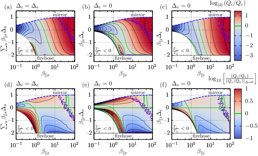
Figure 6: Ratio of ion and electron heating rates, as calculated using (166) for (left) $\Delta_{i}=\Delta_{e}$, (middle) $\Delta_{i}=0$, and (right) $\Delta_{e}=0$ as a function of $\beta_{\parallel s}$ and $\sum_{s}\beta_{\parallel s}\Delta_{s}$. The top row, panels (a)–(c), illustrates the ratio $Q_{i}/Q_{e}$; the bottom row, panels (d)–(e), illustrates this ratio normalized to $Q_{i}/Q_{e}$ evaluated at $\Delta_{s}=0$. The purple contour serves as the boundary above which a finite extent of the Alfvén dispersion relation contains ${\rm Re}(\omega)=0$ modes. See §4.5 for details.

5 Summary

In this paper, we have provided a theoretical framework for describing electromagnetic plasma turbulence in a multi-species, magnetized, pressure-anisotropic plasma characteristic of those found in many space and astrophysical systems. Using linear and nonlinear gyrokinetic theory in concert with the concept of a turbulent cascade of free energy to small scales in phase space, we have arrived at the following principal conclusions:

1. Because of their impact on collisionless damping (see (89)) and the rigidity of magnetic-field lines (see (75)), positive (negative) background pressure anisotropies should shift the ion-Larmor-scale spectral break towards larger (smaller) perpendicular wavenumbers (see (110)). This prediction may be tested by comparing turbulent spectra measured in different parts of the $\beta_{i}\gtrsim 1$ solar wind that exhibit disparate velocity-space anisotropies.

2. The strong ion Landau damping that occurs at the ion-Larmor-scale spectral break for $\beta_{i}\gtrsim 1$ exhibits order-of-magnitude variations in the damping rate depending upon the pressure anisotropy. Since the amount of Landau damping at this scale is related to how much energy ultimately goes into heating the ions or the electrons, pressure anisotropy ought to be considered alongside $\beta_{i}$ and $T_{0i}/T_{0e}$ when assessing the efficiency of ion heating. This is particularly important in the context of radiatively inefficient accretion flows onto supermassive black holes (e.g. Quataert & Gruzinov, 1999), in which the temperature of the electrons is expected to be smaller than the poorly radiating ions and in which pressure anisotropy is thought to play a key role in both the turbulent transport of angular momentum (Quataert et al., 2002; Sharma et al., 2006; Riquelme et al., 2012; Chandra et al., 2015; Hoshino, 2015; Kunz et al., 2016; Foucart et al., 2016) and the non-adiabatic heating of particles (Sharma et al., 2007; Sironi & Narayan, 2015; Sironi, 2015). A generalized version of the Howes (2010) cascade model for assessing ion versus electron heating suggests that ion (electron) heating is enhanced as the mirror (firehose) threshold is approached, with order-of-magnitude variations in $Q_{i}/Q_{e}$ between these thresholds (see figure 6).

3. Kinetic Alfvén waves are subject to both the firehose and mirror instability criteria (see (93)), which, in the sub-ion-Larmor range, are functions of the pressure anisotropy of the electrons only. That the background pressure anisotropy of the ions only affects fluctuations in the inertial range is a consequence of the isothermal pressure response of the ions (see (98a)), which results from the attenuating effect of ring averaging on an otherwise adiabatic response to the fluctuating magnetic-field strength. As a result, Alfvénic fluctuations can be firehose unstable at long ($k_{\perp}\rho_{i}\ll 1$) wavelengths, and yet remain stable at short ($k_{\perp}\rho_{i}\gg 1$) wavelengths. This explains why hybrid-kinetic simulations of firehose and mirror instabilities by Kunz et al. (2014) and of magnetorotational turbulence by Kunz et al. (2016), which used an isothermal and isotropic equation of state for the electrons, demonstrated a KAW cascade at sub-ion-Larmor scales, even though the larger scales were firehose/mirror unstable. In the case where $\beta_{\parallel e}\Delta_{e}<-2$, the KAW is driven unstable to what appears to be the zero-frequency, oblique “electron firehose instability” found by Li & Habbal (2000), for which our work provides a physical explanation and approximate analytical description (§3.6.2).

4. The gyrokinetic system (47), (52)–(54) satisfies the conservation law (118) for the generalized free energy $W_{\rm GK}$ (4.2). In the absence of background interspecies drifts, the conservation of $W_{\rm GK}$ causes a turbulent cascade to small scales in phase space across both the inertial and kinetic range. At long wavelengths, $W_{\rm GK}$ is comprised of two Alfvénic invariants and a compressive invariant, the latter of which is related to the entropy of the perturbed distribution function (Paper I). At short wavelengths, the cascade of $W_{\rm GK}$ splits into an ion-entropy cascade and a KAW cascade, which is governed by the nonlinear equations of ERMHD (modified to include pressure anisotropic species). These cascades are independent of one another so long as $k_{\perp}\rho_{i}\gg 1$ and $\beta_{\perp s}\sim\beta_{\parallel s}\sim 1$, with the ion-entropy cascade taking the collisionlessly damped free energy at the end of the inertial range onwards to collisional scales and the KAW cascade carrying the remainder down to electron scales. In both regimes, as the firehose or mirror instability thresholds are approached, the dynamics of the plasma are modified so as to reduce the energetic cost of bending magnetic-field lines or of compressing them. At $k_{\perp}\rho_{i}\sim 1$, the partitioning of energy into the KAW and ion-entropy cascades is influenced by the strength of the collisionless damping (itself a function of $\beta_{\parallel i}$, $\tau_{\perp{i}}$, $\Delta_{i}$, and $\Delta_{e}$) and the work done by the fluctuating electric and magnetic-mirror forces on the interspecies drifts.

5. Background pressure anisotropy, so long as it remains within the firehose/mirror stability boundaries, does not affect the spectral scaling laws predicted from pressure-isotropic gyrokinetics for strong Alfvénic turbulence in the inertial range (to which the compressive fluctuations are slaved), KAW turbulence in the sub-ion-Larmor range, and the accompanying phase-space cascade of ion entropy to collisional scales (see §4.4). However, it does place constraints on whether scale-dependent pressure anisotropy can be generated and, if so, sustained. We have shown that no scale-dependent electron pressure anisotropy will be generated by compressive fluctuations in either the inertial or kinetic range if no electron pressure anisotropy exists in the background state. By contrast, scale-dependent ion pressure anisotropy can be generated in the inertial range even when $\Delta_{i}=0$, either linearly by the compressive fluctuations (if they are not strongly Landau damped) or nonlinearly by the Alfvénic fluctuations (at second order in the fluctuation amplitude). While the latter source falls out of the range of validity of the gyrokinetic theory that we have developed, it is nevertheless interesting to note that each of these sources will likely produce ion pressure anisotropy with different scaling relations, and that distinguishing between these scaling relations in, say, solar-wind data could help identify the main drivers of fluctuating pressure anisotropy and assess the role of pressure anisotropy in influencing the efficacy of collisionless damping.

In closing, we return to one of the main conclusions of Paper I: that, despite the many quantitative changes arising from the non-Maxwellian nature of the background distribution function, most of the salient qualitative features of the gyrokinetic theory of astrophysical turbulence are robust. This is because, as long as the plasma remains stable, the nature of the nonlinear wave-wave and wave-particle couplings that are central to the theory are insensitive to deviations from velocity-space isotropy, even if the linear physics is not (see Klein & Howes 2015 for an alternate route to the same conclusion). That being said, the study of kinetic turbulence, both theoretical and observational, is becoming increasingly quantitative, and so it is perhaps worth restating Paper I’s coda: “In light of the ever-increasing scrutiny placed upon theories of Alfvénic turbulence by the wealth of data from the solar wind, as well as the astrophysical importance of knowing the proportion of turbulent energy that is distributed between the ion and electron populations, such details matter.” A numerical programme to quantify the broader impact of these details using the theoretical framework developed in this paper is now underway.

Support for M.W.K. was provided by US DOE Contract DE-AC02-09CH11466 and NASA grant NNX16AK09G. Support for I.G.A. was provided by the Princeton Center for Theoretical Science and the Framework grant for Strategic Energy Research (Dnr. 2014-5392) from Vetenskapsrådet. A.A.S. was supported in part by UK STFC Consolidated Grant ST/N000919/1 and ERSPC Grant EP/M022331/1. K.G.K. was supported by NASA grant NNX16AM23G. The authors thank J. Burby, F. Rincon, J. Squire, J. TenBarge, D. Verscharen and especially S. Cowley for useful conversations; G. Howes for providing the code for the cascade model in Howes (2010); and the referees for a careful reading of the manuscript. The completion of this work was facilitated by the generous hospitality and material support provided by the Wolfgang Pauli Institute in Vienna.

Appendix A Definitions of $C^{\perp}_{\ell s}$, $C^{\parallel}_{\ell s}$, $\Gamma^{\perp}_{\ell m}$, and $\Gamma^{\parallel}_{\ell m}$ coefficients

This paper is replete with velocity-space integrals of $f^{\perp}_{0s}$ and $f^{\parallel}_{0s}$ (see (22) for their definitions), which we have allowed to masquerade as deceptively benign coefficients. The first set of these are the $C^{\perp}_{\ell s}$ coefficients:

$$C^{\perp}_{0s} \doteq\frac{1}{n_{0s}}\int{\rm d}^{3}\mbox{\boldmath{$v$}}\,f^{\perp}_{0s},$$ (168a)

$$C^{\perp}_{1s} \doteq\frac{1}{n_{0s}}\int{\rm d}^{3}\mbox{\boldmath{$v$}}\,\frac{v_{\parallel}}{v_{{\rm th}\parallel s}}f^{\perp}_{0s}\times\Biggl{(}\frac{u^{\prime}_{\parallel 0s}}{v_{{\rm th}\parallel s}}\Biggr{)}^{-1},$$ (168b)

$$C^{\perp}_{2s} \doteq\frac{1}{n_{0s}}\int{\rm d}^{3}\mbox{\boldmath{$v$}}\,\frac{v^{2}_{\parallel}}{v_{{\rm th}\parallel s}^{2}}f^{\perp}_{0s}\times\Biggl{(}\frac{1}{2}+\frac{u^{\prime 2}_{\parallel 0s}}{v_{{\rm th}\parallel s}^{2}}\Biggr{)}^{-1},$$ (168c)

normalized so that $C^{\perp}_{\ell s}=1$ for a parallel-drifting bi-Maxwellian distribution function. The next set of coefficients were borne out of the linear theory:

$$C^{\parallel}_{\ell s}(\xi_{s})=\frac{1}{n_{0s}}\int{\rm d}^{3}\mbox{\boldmath{$v$}}\,\frac{1}{\ell!}\biggl{(}\frac{v_{\perp}}{v_{{\rm th}\perp s}}\biggr{)}^{2\ell}\frac{v_{\parallel}-u^{\prime}_{\parallel 0s}}{v_{\parallel}-\omega/k_{\parallel}}f^{\parallel}_{0s}$$ (169)

for integer $\ell$, where $\xi_{s}\doteq(\omega-k_{\parallel}u^{\prime}_{\parallel 0s})/k_{\parallel}v_{{\rm th}\parallel s}$ is the dimensionless Doppler-shifted phase velocity of the (linear) fluctuations. The functions defined by (169) are generalisations of the plasma dispersion function for non-Maxwellian distributions: e.g.

$$C^{\parallel}_{\ell s}(\xi_{s})=1+\xi_{s}Z_{\rm M}(\xi_{s})~{}\textrm{for a bi-Maxwellian, where~{}}Z_{\rm M}(\xi)\doteq\frac{1}{\sqrt{\pi}}\int^{\infty}_{-\infty}{\rm d}x\,\frac{e^{-x^{2}}}{x-\xi}$$ (170)

is the plasma dispersion function (Fried & Conte, 1961).

Accounting for finite-Larmor-radius effects is most easily achieved in the Fourier domain, and the $C_{\ell s}$ coefficients can be profitably generalised by including various combinations of the $n$th-order Bessel function ${\rm J}_{n}(a_{s})$, where $a_{s}\doteq k_{\perp}v_{\parallel}/\Omega_{s}$. Suitably normalised, they are

$$\Gamma_{00}(\alpha_{s}) \doteq\frac{1}{n_{0s}}\int{\rm d}^{3}\mbox{\boldmath{$v$}}\,\bigl{[}{\rm J}_{0}(a_{s})\bigr{]}^{2}\,f_{0s}=1-\alpha_{s}+\dots$$ (171a)

$$\Gamma^{\perp}_{00}(\alpha_{s}) \doteq\frac{1}{n_{0s}}\int{\rm d}^{3}\mbox{\boldmath{$v$}}\,\bigl{[}{\rm J}_{0}(a_{s})\bigr{]}^{2}\,f^{\perp}_{0s}=C^{\perp}_{0s}-\alpha_{s}+\dots$$ (171b)

$$\Gamma^{\perp}_{01}(\alpha_{s}) \doteq\frac{1}{n_{0s}}\int{\rm d}^{3}\mbox{\boldmath{$v$}}\,\bigl{[}{\rm J}_{0}(a_{s})\bigr{]}^{2}\biggl{(}\frac{v_{\parallel}}{v_{{\rm th}\parallel s}}\biggr{)}f^{\perp}_{0s}\times\Biggl{(}\frac{u^{\prime}_{\parallel 0s}}{v_{{\rm th}\parallel s}}\Biggr{)}^{-1}=C^{\perp}_{1s}-\alpha_{s}+\dots$$ (171c)

$$\Gamma^{\perp}_{02}(\alpha_{s}) \doteq\frac{1}{n_{0s}}\int{\rm d}^{3}\mbox{\boldmath{$v$}}\,\bigl{[}{\rm J}_{0}(a_{s})\bigr{]}^{2}\biggl{(}\frac{v_{\parallel}}{v_{{\rm th}\parallel s}}\biggr{)}^{2}f^{\perp}_{0s}\times\Biggl{(}\frac{1}{2}+\frac{u^{\prime 2}_{\parallel 0s}}{v_{{\rm th}\parallel s}^{2}}\Biggr{)}^{-1}=C^{\perp}_{2s}-\alpha_{s}+\dots$$ (171d)

$$\Gamma^{\perp}_{10}(\alpha_{s}) \doteq\frac{1}{n_{0s}}\int{\rm d}^{3}\mbox{\boldmath{$v$}}\,\frac{v^{2}_{\perp}}{v_{{\rm th}\perp s}^{2}}\frac{2{\rm J}_{0}(a_{s}){\rm J}_{1}(a_{s})}{a_{s}}\,f^{\perp}_{0s}=1-\frac{3}{2}\alpha_{s}+\dots$$ (171e)

$$\Gamma^{\perp}_{11}(\alpha_{s}) \doteq\frac{1}{n_{0s}}\int{\rm d}^{3}\mbox{\boldmath{$v$}}\,\frac{v^{2}_{\perp}}{v_{{\rm th}\perp s}^{2}}\frac{2{\rm J}_{0}(a_{s}){\rm J}_{1}(a_{s})}{a_{s}}\biggl{(}\frac{v_{\parallel}}{v_{{\rm th}\parallel s}}\biggr{)}f^{\perp}_{0s}\times\Biggl{(}\frac{u^{\prime}_{\parallel 0s}}{v_{{\rm th}\parallel s}}\Biggr{)}^{-1}=1-\frac{3}{2}\alpha_{s}C_{11s}+\dots$$ (171f)

$$\Gamma^{\perp}_{20}(\alpha_{s}) \doteq\frac{1}{n_{0s}}\int{\rm d}^{3}\mbox{\boldmath{$v$}}\biggl{[}\frac{2v^{2}_{\perp}}{v_{{\rm th}\perp s}^{2}}\frac{{\rm J}_{1}(a_{s})}{a_{s}}\biggr{]}^{2}f^{\perp}_{0s}=2\biggl{(}1-\frac{3}{2}\alpha_{s}C_{20s}+\dots\biggr{)},$$ (171g)

$$\Gamma^{\parallel}_{00}(\xi_{s},\alpha_{s}) \doteq\frac{1}{n_{0s}}\int{\rm d}^{3}\mbox{\boldmath{$v$}}\,\bigl{[}{\rm J}_{0}(a_{s})\bigr{]}^{2}\,\frac{v_{\parallel}-u^{\prime}_{\parallel 0s}}{v_{\parallel}-\omega/k_{\parallel}}f^{\parallel}_{0s}=C^{\parallel}_{0s}(\xi_{s})-\alpha_{s}C^{\parallel}_{1s}(\xi_{s})+\dots,$$ (172a)

$$\Gamma^{\parallel}_{01}(\xi_{s},\alpha_{s}) \doteq\frac{1}{n_{0s}}\int{\rm d}^{3}\mbox{\boldmath{$v$}}\,\bigl{[}{\rm J}_{0}(a_{s})\bigr{]}^{2}\biggl{(}\frac{v_{\parallel}}{v_{{\rm th}\parallel s}}\biggr{)}\frac{v_{\parallel}-u^{\prime}_{\parallel 0s}}{v_{\parallel}-\omega/k_{\parallel}}f^{\parallel}_{0s}\times\Biggl{(}\frac{u^{\prime}_{\parallel 0s}}{v_{{\rm th}\parallel s}}\Biggr{)}^{-1}$$

$$=\frac{\omega}{k_{\parallel}u^{\prime}_{\parallel 0s}}\Gamma^{\parallel}_{00}(\xi_{s},\alpha_{s}),$$ (172b)

$$\Gamma^{\parallel}_{02}(\xi_{s},\alpha_{s}) \doteq\frac{1}{n_{0s}}\int{\rm d}^{3}\mbox{\boldmath{$v$}}\,\bigl{[}{\rm J}_{0}(a_{s})\bigr{]}^{2}\biggl{(}\frac{v_{\parallel}}{v_{{\rm th}\parallel s}}\biggr{)}^{2}\frac{v_{\parallel}-u^{\prime}_{\parallel 0s}}{v_{\parallel}-\omega/k_{\parallel}}f^{\parallel}_{0s}\times\Biggl{(}\frac{1}{2}+\frac{u^{\prime 2}_{\parallel 0s}}{v_{{\rm th}\parallel s}^{2}}\Biggr{)}^{-1}$$

$$=\Biggl{[}\Gamma_{00}(\alpha_{s})+\frac{2u^{\prime 2}_{\parallel 0s}}{v_{{\rm th}\parallel s}^{2}}\frac{\omega^{2}}{k^{2}_{\parallel}u^{\prime 2}_{\parallel 0s}}\Gamma^{\parallel}_{00}(\xi_{s},\alpha_{s})\Biggr{]}\Biggl{(}1+\frac{2u^{\prime 2}_{\parallel 0s}}{v_{{\rm th}\parallel s}^{2}}\Biggr{)}^{-1},$$ (172c)

$$\Gamma^{\parallel}_{10}(\xi_{s},\alpha_{s}) \doteq\frac{1}{n_{0s}}\int{\rm d}^{3}\mbox{\boldmath{$v$}}\,\frac{v^{2}_{\perp}}{v_{{\rm th}\perp s}^{2}}\frac{2{\rm J}_{0}(a_{s}){\rm J}_{1}(a_{s})}{a_{s}}\frac{v_{\parallel}-u^{\prime}_{\parallel 0s}}{v_{\parallel}-\omega/k_{\parallel}}f^{\parallel}_{0s}$$

$$=C^{\parallel}_{1s}(\xi_{s})-\frac{3}{2}\alpha_{s}C^{\parallel}_{2s}(\xi_{s})+\dots,$$ (172d)

$$\Gamma^{\parallel}_{11}(\xi_{s},\alpha_{s}) \doteq\frac{1}{n_{0s}}\int{\rm d}^{3}\mbox{\boldmath{$v$}}\,\frac{v^{2}_{\perp}}{v_{{\rm th}\perp s}^{2}}\frac{2{\rm J}_{0}(a_{s}){\rm J}_{1}(a_{s})}{a_{s}}\biggl{(}\frac{v_{\parallel}}{v_{{\rm th}\parallel s}}\biggr{)}\frac{v_{\parallel}-u^{\prime}_{\parallel 0s}}{v_{\parallel}-\omega/k_{\parallel}}f^{\parallel}_{0s}\times\Biggl{(}\frac{u^{\prime}_{\parallel 0s}}{v_{{\rm th}\parallel s}}\Biggr{)}^{-1}$$

$$=\frac{\omega}{k_{\parallel}u^{\prime}_{\parallel 0s}}\Gamma^{\parallel}_{10}(\xi_{s},\alpha_{s}),$$ (172e)

$$\Gamma^{\parallel}_{20}(\xi_{s},\alpha_{s}) \doteq\frac{1}{n_{0s}}\int{\rm d}^{3}\mbox{\boldmath{$v$}}\,\biggl{[}\frac{2v^{2}_{\perp}}{v_{{\rm th}\perp s}^{2}}\frac{{\rm J}_{1}(\alpha_{s})}{a_{s}}\biggr{]}^{2}\frac{v_{\parallel}-u^{\prime}_{\parallel 0s}}{v_{\parallel}-\omega/k_{\parallel}}f^{\parallel}_{0s}$$

$$=2\biggl{[}C^{\parallel}_{2s}(\xi_{s})-\frac{3}{2}\alpha_{s}C^{\parallel}_{3s}(\xi_{s})+\dots\biggr{]},$$ (172f)

where $\alpha_{s}\doteq(k_{\perp}\rho_{s})^{2}/2$, and

$$C_{11s}\doteq\frac{1}{n_{0s}}\int{\rm d}^{3}\mbox{\boldmath{$v$}}\,\frac{v^{2}_{\perp}}{v_{{\rm th}\perp s}^{2}}\frac{v_{\parallel}}{u^{\prime}_{\parallel 0s}}f_{0s}\quad{\rm and}\quad C_{20s}\doteq\frac{1}{n_{0s}}\int{\rm d}^{3}\mbox{\boldmath{$v$}}\,\frac{1}{2}\frac{v^{4}_{\perp}}{v_{{\rm th}\perp s}^{4}}f_{0s},$$ (173)

both of which equate to unity for a drifting bi-Maxwellian distribution (9). To facilitate comparison with the long-wavelength results of Paper I, the final equalities in (171) and (172) provide their leading-order expansions in $\alpha_{s}\ll 1$. It is helpful to note the numbering scheme used for the $\Gamma_{\ell m}$ subscripts, which reflects the number of powers $\ell$ of $v^{2}_{\perp}$ and $m$ of $v_{\parallel}$ in the integrand.

In §4, we promoted several of these Fourier-space $\Gamma_{\ell m}(\alpha_{s})$ integrals to real-space bi-linear operators by dressing them with hats. Their action on an arbitrary function $\Psi(\mbox{\boldmath{$r$}})=\sum_{\boldsymbol{k}}\Psi_{\boldsymbol{k}}\exp({\rm i}\mbox{\boldmath{$k$}}\,\mbox{\boldmath{$\cdot$}}\,\mbox{\boldmath{$r$}})$ is best expressed in Fourier space:

$$\int{\rm d}^{3}\mbox{\boldmath{$r$}}\,\Psi(\mbox{\boldmath{$r$}})\widehat{\Gamma}_{00}\Psi(\mbox{\boldmath{$r$}}) =\sum_{\boldsymbol{k}}\Gamma_{00}(\alpha_{s})|\Psi_{\boldsymbol{k}}|^{2},$$ (174a)

$$\int{\rm d}^{3}\mbox{\boldmath{$r$}}\,\Psi(\mbox{\boldmath{$r$}})\widehat{\Gamma}^{\perp}_{00}\Psi(\mbox{\boldmath{$r$}}) =\sum_{\boldsymbol{k}}\Gamma^{\perp}_{00}(\alpha_{s})|\Psi_{\boldsymbol{k}}|^{2},$$ (174b)

$$\int{\rm d}^{3}\mbox{\boldmath{$r$}}\,\Psi(\mbox{\boldmath{$r$}})\widehat{\Gamma}^{\perp}_{02}\Psi(\mbox{\boldmath{$r$}}) =\sum_{\boldsymbol{k}}\Gamma^{\perp}_{02}(\alpha_{s})|\Psi_{\boldsymbol{k}}|^{2},$$ (174c)

$$\int{\rm d}^{3}\mbox{\boldmath{$r$}}\,\Psi(\mbox{\boldmath{$r$}})\widehat{\Gamma}^{\perp}_{11}\Psi(\mbox{\boldmath{$r$}}) =\sum_{\boldsymbol{k}}\Gamma^{\perp}_{11}(\alpha_{s})|\Psi_{\boldsymbol{k}}|^{2},$$ (174d)

$$\int{\rm d}^{3}\mbox{\boldmath{$r$}}\,\Psi(\mbox{\boldmath{$r$}})\widehat{\Gamma}^{\parallel}_{20}\Psi(\mbox{\boldmath{$r$}}) =\sum_{\boldsymbol{k}}\Gamma^{\parallel}_{20}(0,\alpha_{s})|\Psi_{\boldsymbol{k}}|^{2},$$ (174e)

$$\int{\rm d}^{3}\mbox{\boldmath{$r$}}\,\Psi(\mbox{\boldmath{$r$}})\widehat{\Gamma}^{\perp}_{20}\Psi(\mbox{\boldmath{$r$}}) =\sum_{\boldsymbol{k}}\Gamma^{\perp}_{20}(\alpha_{s})|\Psi_{\boldsymbol{k}}|^{2}$$ (174f)

with the Fourier-space $\Gamma_{\ell m}(\alpha_{s})$ integrals being given by (171a,b,d,f,g) and (172f).

This completes our catalogue of integrals.

Appendix B Limiting cases of the bi-Maxwellian linear gyrokinetic dispersion relation

In this appendix, the transition between the long-wavelength solutions of §3.6.1 and the short-wavelength solutions of §3.6.2 is treated in the analytically tractable limits of high and low $\beta_{\parallel i}$. This follows the procedure in appendix of D Howes et al. (2006) of identifying the analytically solvable cases.

B.1 High-$\beta_{\parallel i}$ limit: $\beta_{\parallel i}\gg 1$, $k_{\perp}\rho_{i}\sim 1$

For $\beta_{\parallel i}\gg 1$, we have $\xi_{i}=\overline{\omega}/\beta_{\parallel i}^{1/2}\ll 1$ and $\xi_{e}=(m_{e}/m_{i})^{1/2}(T_{\parallel 0{i}}/T_{\parallel 0{e}})^{1/2}\xi_{i}\ll 1$, and we can use the small-argument expansion of the plasma dispersion function, $Z_{\rm M}(\xi_{s})\simeq{\rm i}\sqrt{\pi}$. This requires $\tau_{\parallel{i}}\ll(m_{i}/m_{e})\beta_{\parallel i}$, which is not particularly restrictive. We also take $\alpha_{e}\ll 1$ because $m_{e}/m_{i}\ll 1$, as well as order the pressure anisotropy $\Delta_{s}\sim 1/\beta_{\parallel s}$. Retaining $k_{\perp}\rho_{i}\sim 1$, the coefficients of the gyrokinetic dispersion relation (81) become

$$\mathcal{A} \simeq 1+\Gamma_{0}(\alpha_{i})\Delta_{i}+\frac{\tau_{\perp{i}}}{Z_{i}}\frac{T_{\perp 0{e}}}{T_{\parallel 0{e}}}+{\rm i}\sqrt{\pi}\,\xi_{i}\,\frac{T_{\perp 0{i}}}{T_{\parallel 0{i}}}\Biggl{[}\Gamma_{0}(\alpha_{i})+\biggl{(}\frac{\tau_{\parallel{i}}}{Z_{i}}\biggr{)}^{3/2}\biggl{(}\frac{Z_{i}m_{e}}{m_{i}}\biggr{)}^{1/2}\Biggr{]},$$ (175a)

$$\mathcal{B} \simeq 1-\Gamma_{0}(\alpha_{i}),$$ (175b)

$$\mathcal{C} \simeq\Gamma_{1}(\alpha_{i})\Delta_{i}-\Delta_{e}+{\rm i}\sqrt{\pi}\,\xi_{i}\,\frac{T_{\perp 0{i}}}{T_{\parallel 0{i}}}\Biggl{[}\Gamma_{1}(\alpha_{i})-\frac{\tau_{\parallel{i}}}{\tau_{\perp{i}}}\biggl{(}\frac{\tau_{\parallel{i}}}{Z_{i}}\frac{Z_{i}m_{e}}{m_{i}}\biggr{)}^{1/2}\Biggr{]},$$ (175c)

$$\mathcal{D} \simeq 2\biggl{[}\Gamma_{1}(\alpha_{i})\Delta_{i}+\frac{Z_{i}}{\tau_{\perp{i}}}\Delta_{e}\biggr{]}+2{\rm i}\sqrt{\pi}\,\xi_{i}\,\frac{T_{\perp 0{i}}}{T_{\parallel 0{i}}}\Biggl{[}\Gamma_{1}(\alpha_{i})+\frac{\tau_{\parallel{i}}^{2}}{\tau_{\perp{i}}^{2}}\biggl{(}\frac{Z_{i}}{\tau_{\parallel{i}}}\frac{Z_{i}m_{e}}{m_{i}}\biggr{)}^{1/2}\Biggr{]}$$

$$\doteq\frac{2}{\beta_{\perp i}}\bigl{[}1-\mathcal{F}(\alpha_{i})\bigr{]}+2{\rm i}\sqrt{\pi}\,\xi_{i}\mathcal{G}(\alpha_{i}),$$ (175d)

$$\mathcal{E} \simeq\Gamma_{1}(\alpha_{i})-1,$$ (175e)

where we have dropped all terms of first order and higher in $Z_{i}m_{e}/m_{i}$. As in §3.6.2, we must be careful to retain the final term in the definition of $\alpha_{\ast}$ (81f), despite its dependence on the higher-order $1-\Gamma_{0}(\alpha_{e})$ factor. The auxiliary functions $\mathcal{F}(\alpha_{i})$ and $\mathcal{G}(\alpha_{i})$, which are defined implicitly by (175d), will become useful below.

We proceed by taking two instructive limits.

B.1.1 The limit $k_{\perp}\rho_{i}\sim\mathcal{O}(\beta_{\parallel i}^{-1/4})$, $\overline{\omega}\sim\mathcal{O}(1)$

In this ordering, we have $\alpha_{i}\sim\xi_{i}\sim\mathcal{O}(\beta_{\parallel i}^{-1/2})$, and so we may expand $\Gamma_{0}(\alpha_{i})\simeq 1-\alpha_{i}$ and $\Gamma_{1}(\alpha_{i})\simeq 1-(3/2)\alpha_{i}$. We find from (175) that $\mathcal{A}\sim\mathcal{O}(1)$ and $\mathcal{B}$, $\mathcal{C}$, $\mathcal{D}$, and $\mathcal{E}\sim\mathcal{O}(\beta_{\parallel i}^{-1/2})$. Then, the dispersion relation (82) becomes

$$-\biggl{(}\frac{\alpha_{\ast}}{\overline{\omega}^{2}}-\mathcal{B}\biggr{)}\mathcal{D}=\mathcal{E}^{2},$$ (176)

where, to leading order, we have $\mathcal{B}\simeq\alpha_{i}$, $\mathcal{E}\simeq-(3/2)\alpha_{i}$, $\mathcal{D}\simeq 2{\rm i}\overline{\omega}(\pi/\beta_{\parallel i})^{1/2}$, and $\alpha_{\ast}\simeq\alpha_{i}[1+(\beta_{\parallel i}/2)\Delta_{i}+(\beta_{\parallel e}/2)\Delta_{e}]$. This is a quadratic equation for $\overline{\omega}$, whose solutions are

$$\overline{\omega}=-{\rm i}\frac{9}{16}\sqrt{\frac{\beta_{\parallel i}}{\pi}}\alpha_{i}\pm\sqrt{1+\frac{\beta_{\parallel i}}{2}\Delta_{i}+\frac{\beta_{\parallel e}}{2}\Delta_{e}-\Biggr{(}\frac{9}{16}\sqrt{\frac{\beta_{\parallel i}}{\pi}}\alpha_{i}\Biggr{)}^{2}}.$$ (177)

In the subsidiary limit, $k_{\perp}\rho_{i}\ll 1/\beta_{\parallel i}^{1/4}$, we recover, as expected, the Alfvén wave, now with weak collisionless damping (cf. (84)):

$$\overline{\omega}=\pm\sqrt{1+\frac{\beta_{\parallel i}}{2}\Delta_{i}+\frac{\beta_{\parallel e}}{2}\Delta_{e}}-{\rm i}\frac{9}{16}\frac{k^{2}_{\perp}\rho^{2}_{i}}{2}\sqrt{\frac{\beta_{\parallel i}}{\pi}}.$$ (178)

In the intermediate asymptotic limit $\beta_{\parallel i}^{-1/4}\ll k_{\perp}\rho_{i}\ll 1$, we have two solutions:

$$\overline{\omega} =-{\rm i}\frac{8}{9}\biggl{(}1+\frac{\beta_{\parallel i}}{2}\Delta_{i}+\frac{\beta_{\parallel e}}{2}\Delta_{e}\biggr{)}\biggl{(}\frac{k^{2}_{\perp}\rho^{2}_{i}}{2}\biggr{)}^{-1}\sqrt{\frac{\pi}{\beta_{\parallel i}}}\qquad\textrm{(weakly damped)};$$ (179a)

$$\overline{\omega} =-{\rm i}\frac{9}{8}\frac{k^{2}_{\perp}\rho^{2}_{i}}{2}\sqrt{\frac{\beta_{\parallel i}}{\pi}}\qquad\textrm{(strongly damped)}.$$ (179b)

B.1.2 The limit $k_{\perp}\rho_{i}\sim\mathcal{O}(1)$, $\overline{\omega}\sim\mathcal{O}(\beta_{\parallel i}^{-1/2})$

In this ordering, $\alpha_{i}\sim\mathcal{O}(1)$ and $\xi_{i}\sim\mathcal{O}(\beta_{\parallel i}^{-1})$. Then $\mathcal{A}$, $\mathcal{B}$, $\mathcal{E}\sim\mathcal{O}(1)$, and $\mathcal{C}$, $\mathcal{D}\sim\mathcal{O}(\beta_{\parallel i}^{-1})$. The dispersion relation (82) becomes

$$\frac{\alpha_{\ast}}{\overline{\omega}^{2}}\biggl{(}\frac{2}{\beta_{\perp i}}-\mathcal{D}\biggr{)}=\mathcal{E}^{2}.$$ (180)

Since $\mathcal{D}\simeq(2/\beta_{\perp i})[1-\mathcal{F}(\alpha_{i})]+2{\rm i}\sqrt{\pi}\,\xi_{i}\mathcal{G}(\alpha_{i})$, this is again a quadratic equation for $\overline{\omega}$, with solutions given by

$$\overline{\omega}=-{\rm i}\sqrt{\frac{\pi}{\beta_{\parallel i}}}\frac{\alpha_{\ast}\,\mathcal{G}(\alpha_{i})}{\bigl{[}\Gamma_{1}(\alpha_{i})-1\bigr{]}^{2}}\pm\sqrt{\frac{2}{\beta_{\perp i}}\frac{\alpha_{\ast}\,\mathcal{F}(\alpha_{i})}{\bigl{[}\Gamma_{1}(\alpha_{i})-1\bigr{]}^{2}}-\Biggl{\{}\sqrt{\frac{\pi}{\beta_{\parallel i}}}\frac{\alpha_{\ast}\,\mathcal{G}(\alpha_{i})}{\bigl{[}\Gamma_{1}(\alpha_{i})-1\bigr{]}^{2}}\Biggr{\}}^{2}}.$$ (181)

In the long-wavelength limit, $k_{\perp}\rho_{i}\ll 1$, these become

$$\overline{\omega} =-\frac{{\rm i}}{\sqrt{\pi\beta_{\parallel i}}}\frac{T_{\parallel 0{i}}^{2}}{T_{\perp 0{i}}^{2}}\Bigl{(}1-\beta_{\perp i}\Delta_{i}-\beta_{\perp e}\Delta_{e}\Bigr{)},$$ (182a)

$$\overline{\omega} =-{\rm i}\frac{8}{9}\biggl{(}1+\frac{\beta_{\parallel i}}{2}\Delta_{i}+\frac{\beta_{\parallel e}}{2}\Delta_{e}\biggr{)}\biggl{(}\frac{k^{2}_{\perp}\rho^{2}_{i}}{2}\biggr{)}^{-1}\sqrt{\frac{\pi}{\beta_{\parallel i}}}\frac{T_{\perp 0{i}}}{T_{\parallel 0{i}}}.$$ (182b)

The first solution is the Barnes-damped (or mirror-unstable) slow wave (cf. I–4.33); the second solution matches the weakly damped Alfvén wave in the intermediate limit (see (179a)).

In the subsidiary short-wavelength limit, $k_{\perp}\rho_{i}\gg 1$, we have $\Gamma_{1}(\alpha_{i})\rightarrow 0$, $\mathcal{F}(\alpha_{i})\rightarrow 1-\beta_{\perp e}\Delta_{e}$, and $\mathcal{G}(\alpha_{i})\rightarrow(T_{\perp 0{e}}/T_{\parallel 0{e}})(\tau_{\parallel{i}}/\tau_{\perp{i}})(Z_{i}/\tau_{\parallel{i}})^{1/2}(Z_{i}m_{e}/m_{i})^{1/2}$. Then (181) reproduces the $\beta_{\parallel i}\gg 1$ limit of the KAW dispersion relation (cf. 93):

$$\overline{\omega} =\pm\frac{k_{\perp}\rho_{i}}{\sqrt{\beta_{\perp i}}}\biggl{(}1+\frac{\beta_{\parallel e}}{2}\Delta_{e}\biggr{)}^{1/2}\Bigl{(}1-\beta_{\perp e}\Delta_{e}\Bigr{)}^{1/2}$$

$$-{\rm i}\frac{k^{2}_{\perp}\rho^{2}_{i}}{2}\sqrt{\frac{\pi}{\beta_{\parallel i}}}\biggl{(}1+\frac{\beta_{\parallel e}}{2}\Delta_{e}\biggr{)}\frac{T_{\perp 0{e}}}{T_{\parallel 0{e}}}\frac{\tau_{\parallel{i}}}{\tau_{\perp{i}}}\biggl{(}\frac{Z_{i}}{\tau_{\parallel{i}}}\frac{Z_{i}m_{e}}{m_{i}}\biggr{)}^{1/2}.$$ (183)

B.2 Low-$\beta_{\parallel i}$ limit: $\beta_{\parallel i}\ll 1$, $k_{\perp}\rho_{i}\sim 1$

For $\beta_{\parallel i}\ll 1$ and $\Delta_{s}\sim 1$, the coefficients $\mathcal{A}$, $\mathcal{B}$, $\mathcal{C}$, $\mathcal{D}$, $\mathcal{E}\sim\mathcal{O}(1)$. Then the gyrokinetic dispersion relation (82) reduces to

$$\biggl{(}\frac{\alpha_{\ast}\mathcal{A}}{\overline{\omega}^{2}}-\mathcal{A}\mathcal{B}+\mathcal{B}^{2}\biggr{)}\frac{2\mathcal{A}}{\beta_{\perp i}}=0.$$ (184)

The long-wavelength limit of the second factor ($\mathcal{A}=0$) gives the Landau-damped ion acoustic wave (see (LABEL:eqn:ionacoustic)). For the first factor, we order $\overline{\omega}\sim\mathcal{O}(1)$ and consider two interesting limits:

B.2.1 The limit $(Z_{i}m_{e}/m_{i})(\tau_{\perp{i}}/Z_{i})\ll\beta_{\parallel i}\ll 1$

In this limit, $\xi_{i}=\overline{\omega}/\sqrt{\beta_{\parallel i}}\gg 1$ and $\xi_{e}=(Z_{i}m_{e}/m_{i})^{1/2}(\tau_{\perp{i}}/Z_{i})^{1/2}\ll 1$ (slow ions, fast electrons). Expanding the ion and electron plasma dispersion functions in large and small arguments, respectively, we get

$$\mathcal{A} \simeq 1-\Gamma_{0}(\alpha_{i})+\frac{\tau_{\perp{i}}}{Z_{i}}\bigl{[}1+\Gamma_{0}(\alpha_{e})\Delta_{e}\bigr{]}$$

$$+{\rm i}\overline{\omega}\sqrt{\frac{\pi}{\beta_{\parallel i}}}\frac{T_{\perp 0{i}}}{T_{\parallel 0{i}}}\Biggl{[}\Gamma_{0}(\alpha_{i})\exp\biggl{(}-\frac{\overline{\omega}^{2}}{\beta_{\parallel i}}\biggr{)}+\biggl{(}\frac{\tau_{\parallel{i}}}{Z_{i}}\biggr{)}^{3/2}\biggl{(}\frac{Z_{i}m_{e}}{m_{i}}\biggr{)}^{1/2}\Gamma_{0}(\alpha_{e})\Biggr{]}.$$ (185)

The dispersion relation (184) then becomes

$$\frac{\tau_{\perp{i}}}{Z_{i}}\frac{T_{\perp 0{e}}}{T_{\parallel 0{e}}}\mathcal{B}\Gamma_{0}(\alpha_{e})\overline{\omega}^{2}-\alpha_{\ast}\biggl{\{}1-\Gamma_{0}(\alpha_{i})+\frac{\tau_{\perp{i}}}{Z_{i}}\bigl{[}1+\Delta_{e}\Gamma_{0}(\alpha_{e})\bigr{]}\biggr{\}}=-{\rm i}\bigl{(}\mathcal{B}\overline{\omega}^{2}-\alpha_{\ast}\bigr{)}{\rm Im}(\mathcal{A}).$$ (186)

This equation may be iteratively solved to find

$${\rm Re}(\overline{\omega}) =\pm\sqrt{\frac{\alpha_{\ast}\bigl{\{}1-\Gamma_{0}(\alpha_{i})+(\tau_{\perp{i}}/Z_{i})\bigl{[}1+\Delta_{e}\Gamma_{0}(\alpha_{e})\bigr{]}\bigr{\}}}{(\tau_{\perp{i}}/Z_{i})(T_{\perp 0{e}}/T_{\parallel 0{e}})\mathcal{B}\Gamma_{0}(\alpha_{e})}},$$ (187a)

$$\overline{\gamma} =-\frac{\alpha_{\ast}}{2\bigl{[}(\tau_{\parallel{i}}/Z_{i})\Gamma_{0}(\alpha_{e})\bigr{]}^{2}}\sqrt{\frac{\pi}{\beta_{\parallel i}}}\frac{T_{\parallel 0{i}}}{T_{\perp 0{i}}}$$

$$\quad\times\Biggl{[}\Gamma_{0}(\alpha_{i})\exp\biggl{(}-\frac{\overline{\omega}^{2}}{\beta_{\parallel i}}\biggr{)}+\biggl{(}\frac{\tau_{\parallel{i}}}{Z_{i}}\biggr{)}^{3/2}\biggl{(}\frac{Z_{i}m_{e}}{m_{i}}\biggr{)}^{1/2}\Gamma_{0}(\alpha_{e})\Biggr{]},$$ (187b)

where $\overline{\gamma}\doteq{\rm Im}(\omega)/k_{\parallel}v_{\rm A}$. In the limit $\alpha_{i}\ll 1$, (187a) reduces to the Alfvén wave solution (84).

B.2.2 The limit $\beta_{\parallel i}\sim Z_{i}m_{e}/m_{i}\ll 1$, $\tau_{\perp{i}}/Z_{i}\gg 1$

In this limit, $\xi_{i}\sim(m_{i}/m_{e})^{1/2}\gg 1$, and so $\xi_{e}\sim(\tau_{\perp{i}}/Z_{i})^{1/2}\gg 1$ (cold ions and electrons). Expanding all plasma dispersion functions in their large arguments, the coefficient

$$\mathcal{A} \simeq\mathcal{B}-\frac{\Gamma_{0}(\alpha_{e})}{2\overline{\omega}^{2}}\frac{m_{i}}{Z_{i}m_{e}}\beta_{\perp i}+{\rm i}\overline{\omega}\sqrt{\frac{\pi}{\beta_{\parallel i}}}\frac{T_{\perp 0{i}}}{T_{\parallel 0{i}}}$$

$$\times\Biggl{[}\Gamma_{0}(\alpha_{i})\exp\biggl{(}-\frac{\overline{\omega}^{2}}{\beta_{\parallel i}}\biggr{)}+\biggl{(}\frac{\tau_{\parallel{i}}}{Z_{i}}\biggr{)}^{3/2}\biggl{(}\frac{Z_{i}m_{e}}{m_{i}}\biggr{)}^{1/2}\Gamma_{0}(\alpha_{e})\exp\biggl{(}-\frac{T_{\parallel 0{i}}}{T_{\parallel 0{e}}}\frac{m_{e}}{m_{i}}\frac{\overline{\omega}^{2}}{\beta_{\parallel i}}\biggr{)}\Biggr{]}.$$ (188)

The dispersion relation (184) then becomes

$$\frac{\alpha_{\ast}\Gamma_{0}(\alpha_{e})}{2\overline{\omega}^{2}}\frac{m_{i}}{Z_{i}m_{e}}\beta_{\perp i}-\mathcal{B}\biggl{[}\alpha_{\ast}+\frac{\Gamma_{0}(\alpha_{e})}{2}\frac{m_{i}}{Z_{i}m_{e}}\beta_{\perp i}\biggr{]}=-{\rm i}\bigl{(}\mathcal{B}\overline{\omega}^{2}-\alpha_{\ast}\bigr{)}{\rm Im}(\mathcal{A}),$$ (189)

which may be iteratively solved to find

$$\overline{\omega} =\pm\sqrt{\frac{\alpha_{\ast}\Gamma_{0}(\alpha_{e})(m_{i}/Z_{i}m_{e})\beta_{\perp i}}{\bigl{[}2\alpha_{\ast}+\Gamma_{0}(\alpha_{e})(m_{i}/Z_{i}m_{e})\beta_{\perp i}\bigr{]}\mathcal{B}}},$$ (190a)

$$\overline{\gamma} =-\frac{2\alpha^{3}_{\ast}\Gamma_{0}(\alpha_{e})(m_{i}/Z_{i}m_{e})\beta_{\perp i}}{\bigl{[}2\alpha_{\ast}+\Gamma_{0}(\alpha_{e})(m_{i}/Z_{i}m_{e})\beta_{\perp i}\bigr{]}^{3}\mathcal{B}^{2}}\sqrt{\frac{\pi}{\beta_{\parallel i}}}\frac{T_{\perp 0{i}}}{T_{\parallel 0{i}}}$$

$$\times\Biggl{[}\Gamma_{0}(\alpha_{i})\exp\biggl{(}-\frac{\overline{\omega}^{2}}{\beta_{\parallel i}}\biggr{)}+\biggl{(}\frac{\tau_{\parallel{i}}}{Z_{i}}\biggr{)}^{3/2}\biggl{(}\frac{Z_{i}m_{e}}{m_{i}}\biggr{)}^{1/2}\Gamma_{0}(\alpha_{e})\exp\biggl{(}-\frac{T_{\parallel 0{i}}}{T_{\parallel 0{e}}}\frac{m_{e}}{m_{i}}\frac{\overline{\omega}^{2}}{\beta_{\parallel i}}\biggr{)}\Biggr{]}.$$ (190b)

B.3 Gyrokinetic dispersion relation for an electron-ion bi-kappa plasma

A bi-kappa distribution function is often used to describe the non-thermal electron population in the solar wind and, in particular, its suprathermal ($T_{e}\sim 60~{}{\rm eV}$) halo (see, e.g. Vasyliunas, 1968; Maksimovic et al., 1997a, b, 2005). In this section, we specialize the linear gyrokinetic theory of §§3.2 and 3.3 to a mean distribution function equal to

$$f_{\textrm{bi-}\kappa,s}(v_{\parallel},v_{\perp})\doteq\frac{n_{0s}}{\sqrt{\pi\kappa}\theta_{\parallel s}}\frac{1}{\pi\kappa\theta^{2}_{\perp s}}\frac{\Gamma(\kappa+1)}{\Gamma(\kappa-1/2)}\Biggl{[}1+\frac{(v_{\parallel}-u^{\prime}_{\parallel 0s})^{2}}{\kappa\theta^{2}_{\parallel s}}+\frac{v^{2}_{\perp}}{\kappa\theta^{2}_{\perp s}}\Biggr{]}^{-(\kappa+1)},$$ (191)

where $\Gamma$ is the Gamma function, $\kappa>3/2$ is the spectral index, and

$$\theta_{\parallel s}\doteq v_{{\rm th}\parallel s}\sqrt{1-\frac{3}{2\kappa}}\quad{\rm and}\quad\theta_{\perp s}\doteq v_{{\rm th}\perp s}\sqrt{1-\frac{3}{2\kappa}}$$ (192)

are the effective parallel and perpendicular thermal speeds, respectively. At low and thermal energies, the bi-kappa distribution approaches a Maxwellian distribution, whereas at high energies it exhibits a non-thermal tail that can be described as a decreasing power law. The $C_{\ell s}$ coefficients are evaluated for $f_{\textrm{bi-}\kappa,s}$ in appendix D of Paper I.

The changes to the results presented in §§3.6, 4.3, 4.4 made by instead using a bi-kappa background distribution function are only quantitative. For example, the dispersion relation for the KAW (93) becomes

$$\omega=\pm\frac{k_{\parallel}v_{\rm A}k_{\perp}\rho_{i}}{\sqrt{\beta_{\perp i}+2/(1+Z_{i}T_{\parallel 0{e}}/T_{\perp 0{i}})-2\mathcal{K}_{\kappa}}}\biggl{(}1+\frac{\beta_{\parallel e}}{2}\Delta_{e}\biggr{)}^{1/2}\biggl{(}1-\beta_{\perp e}\Delta_{e}+\frac{\mathcal{K}}{C_{\kappa}}\biggr{)}^{1/2},$$ (193)

where

$$\mathcal{K}_{\kappa}\doteq\mathcal{K}\,\frac{(2C_{\kappa}-1)T_{\perp 0{e}}/T_{\parallel 0{e}}-1}{T_{\perp 0{e}}/T_{\parallel 0{e}}-1}\quad{\rm and}\quad C_{\kappa}\doteq\biggl{(}1-\frac{1}{2\kappa}\biggr{)}\biggl{(}1-\frac{3}{2\kappa}\biggr{)}^{-1}.$$ (194)

The modification is due to the effect of high-parallel-energy particles in the tail of the $\kappa$ distribution on the mirror stability threshold: a smaller fraction of particles are Landau resonant and thus the stabilizing influence of the parallel electric field on the mirror instability is reduced.

References

- Alexandrova et al. (2009) Alexandrova, O., Saur, J., Lacombe, C., Mangeney, A., Mitchell, J., Schwartz, S. J. & Robert, P. 2009 Universality of Solar-Wind Turbulent Spectrum from MHD to Electron Scales. Phys. Rev. Lett. 103 (16), 165003.
- Antonsen & Lane (1980) Antonsen, Jr., T. M. & Lane, B. 1980 Kinetic equations for low frequency instabilities in inhomogeneous plasmas. Phys. Fluids 23, 1205–1214.
- Armstrong et al. (1990) Armstrong, J. W., Coles, W. A., Rickett, B. J. & Kojima, M. 1990 Observations of field-aligned density fluctuations in the inner solar wind. Astrophys. J. 358, 685–692.
- Arzamasskiy et al. (2018) Arzamasskiy, L., Kunz, M. W., Chandran, B. D. G. & Quataert, E. 2018 . in prep. .
- Bale et al. (2005) Bale, S. D., Kellogg, P. J., Mozer, F. S., Horbury, T. S. & Reme, H. 2005 Measurement of the Electric Fluctuation Spectrum of Magnetohydrodynamic Turbulence. Phys. Rev. Lett. 94 (21), 215002.
- Barnes (1966) Barnes, A. 1966 Collisionless Damping of Hydromagnetic Waves. Phys. Fluids 9, 1483–1495.
- Bavassano et al. (2004) Bavassano, B., Pietropaolo, E. & Bruno, R. 2004 Compressive fluctuations in high-latitude solar wind. Ann. Geophys. 22, 689–696.
- Belcher & Davis (1971) Belcher, J. W. & Davis, L., Jr. 1971 Large-Amplitude Alfvén Waves in the Interplanetary Medium, 2. J. Geophys. Res. 76, 3534–3563.
- Bieber et al. (1996) Bieber, J. W., Wanner, W. & Matthaeus, W. H. 1996 Dominant two-dimensional solar wind turbulence with implications for cosmic ray transport. J. Geophys. Res. 101, 2511–2522.
- Boldyrev (2006) Boldyrev, S. 2006 Spectrum of Magnetohydrodynamic Turbulence. Phys. Rev. Lett. 96 (11), 115002.
- Boldyrev & Perez (2012) Boldyrev, S. & Perez, J. C. 2012 Spectrum of Kinetic-Alfvén Turbulence. Astrophys. J. Lett. 758, L44.
- Brizard (1994) Brizard, A. J. 1994 Quadratic free energy for the linearized gyrokinetic Vlasov-Maxwell equations. Phys. Plasmas 1, 2473–2479.
- Brizard & Hahm (2007) Brizard, A. J. & Hahm, T. S. 2007 Foundations of nonlinear gyrokinetic theory. Rev. Mod. Phys. 79, 421–468.
- Bruno & Carbone (2005) Bruno, R. & Carbone, V. 2005 The Solar Wind as a Turbulence Laboratory. Living Reviews in Solar Physics 2, 4.
- Burlaga et al. (1990) Burlaga, L. F., Scudder, J. D., Klein, L. W. & Isenberg, P. A. 1990 Pressure-balanced structures between 1 AU and 24 AU and their implications for solar wind electrons and interstellar pickup ions. J. Geophys. Res. 95, 2229–2239.
- Catto (1978) Catto, P. J. 1978 Linearized gyro-kinetics. Plasma Physics 20, 719–722.
- Catto et al. (1981) Catto, P. J., Tang, W. M. & Baldwin, D. E. 1981 Generalized gyrokinetics. Plasma Physics 23, 639–650.
- Cerri et al. (2016) Cerri, S. S., Califano, F., Jenko, F., Told, D. & Rincon, F. 2016 Subproton-scale Cascades in Solar Wind Turbulence: Driven Hybrid-kinetic Simulations. Astrophys. J. Lett. 822, L12.
- Cerri et al. (2017a) Cerri, S. S., Franci, L., Califano, F., Landi, S. & Hellinger, P. 2017a Plasma turbulence at ion scales: a comparison between particle in cell and Eulerian hybrid-kinetic approaches. J. Plasma Phys. 83 (2), 705830202.
- Cerri et al. (2017b) Cerri, S. S., Servidio, S. & Califano, F. 2017b Kinetic Cascade in Solar-wind Turbulence: 3D3V Hybrid-kinetic Simulations with Electron Inertia. Astrophys. J. Lett. 846, L18.
- Chandra et al. (2015) Chandra, M., Gammie, C. F., Foucart, F. & Quataert, E. 2015 An Extended Magnetohydrodynamics Model for Relativistic Weakly Collisional Plasmas. Astrophys. J. 810, 162.
- Chandran et al. (2010) Chandran, B. D. G., Li, B., Rogers, B. N., Quataert, E. & Germaschewski, K. 2010 Perpendicular Ion Heating by Low-frequency Alfvén-wave Turbulence in the Solar Wind. Astrophys. J. 720, 503–515.
- Chandran et al. (2015) Chandran, B. D. G., Schekochihin, A. A. & Mallet, A. 2015 Intermittency and Alignment in Strong RMHD Turbulence. Astrophys. J. 807, 39.
- Chandran et al. (2013) Chandran, B. D. G., Verscharen, D., Quataert, E., Kasper, J. C., Isenberg, P. A. & Bourouaine, S. 2013 Stochastic Heating, Differential Flow, and the Alpha-to-proton Temperature Ratio in the Solar Wind. Astrophys. J. 776, 45.
- Chen (2016) Chen, C. H. K. 2016 Recent progress in astrophysical plasma turbulence from solar wind observations. J. Plasma Phys. 82 (6), 535820602.
- Chen et al. (2014) Chen, C. H. K., Leung, L., Boldyrev, S., Maruca, B. A. & Bale, S. D. 2014 Ion-scale spectral break of solar wind turbulence at high and low beta. Geophys. Res. Lett. 41, 8081–8088.
- Chen et al. (2011) Chen, C. H. K., Mallet, A., Yousef, T. A., Schekochihin, A. A. & Horbury, T. S. 2011 Anisotropy of Alfvénic turbulence in the solar wind and numerical simulations. Mon. Not. R. Astron. Soc. 415, 3219–3226.
- Chew et al. (1956) Chew, G. F., Goldberger, M. L. & Low, F. E. 1956 The Boltzmann Equation and the One-Fluid Hydromagnetic Equations in the Absence of Particle Collisions. Proc. R. Soc. London A 236, 112–118.
- Cho & Lazarian (2004) Cho, J. & Lazarian, A. 2004 The anisotropy of electron magnetohydrodynamic turbulence. Astrophys. J. 615, L41.
- Cho & Vishniac (2000) Cho, J. & Vishniac, E. T. 2000 The Anisotropy of Magnetohydrodynamic Alfvénic Turbulence. Astrophys. J. 539, 273–282.
- Cranmer (2014) Cranmer, S. R. 2014 Ensemble Simulations of Proton Heating in the Solar Wind via Turbulence and Ion Cyclotron Resonance. Astrophys. J. Supp. Ser. 213, 16.
- Davidson & Völk (1968) Davidson, R. C. & Völk, H. J. 1968 Macroscopic Quasilinear Theory of the Garden-Hose Instability. Phys. Fluids 11, 2259–2264.
- Dmitruk et al. (2004) Dmitruk, P., Matthaeus, W. H. & Seenu, N. 2004 Test Particle Energization by Current Sheets and Nonuniform Fields in Magnetohydrodynamic Turbulence. Astrophys. J. 617, 667–679.
- Dubin et al. (1983) Dubin, D. H. E., Krommes, J. A., Oberman, C. & Lee, W. W. 1983 Nonlinear gyrokinetic equations. Phys. Fluids 26, 3524.
- Feldman et al. (1973) Feldman, W. C., Asbridge, J. R., Bame, S. J. & Montgomery, M. D. 1973 Double ion streams in the solar wind. J. Geophys. Res. 78, 2017.
- Foucart et al. (2016) Foucart, F., Chandra, M., Gammie, C. F. & Quataert, E. 2016 Evolution of accretion discs around a kerr black hole using extended magnetohydrodynamics. Mon. Not. R. Astron. Soc. 456, 1332–1345.
- Fowler (1968) Fowler, T. K. 1968 Thermodynamics of Unstable Plasmas. Advances in Plasma Physics 1, 201.
- Franci et al. (2015a) Franci, L., Landi, S., Matteini, L., Verdini, A. & Hellinger, P. 2015a High-resolution Hybrid Simulations of Kinetic Plasma Turbulence at Proton Scales. Astrophys. J. 812, 21.
- Franci et al. (2016) Franci, L., Landi, S., Matteini, L., Verdini, A. & Hellinger, P. 2016 Plasma Beta Dependence of the Ion-scale Spectral Break of Solar Wind Turbulence: High-resolution 2D Hybrid Simulations. Astrophys. J. 833, 91.
- Franci et al. (2017) Franci, L., Landi, S., Verdini, A., Mattini, L. & Hellinger, P. 2017 Solar wind turbulent cascade from MHD to sub-ion scales: large-size 3D hybrid particle-in-cell simulations. ArXiv e-prints .
- Franci et al. (2015b) Franci, L., Verdini, A., Matteini, L., Landi, S. & Hellinger, P. 2015b Solar Wind Turbulence from MHD to Sub-ion Scales: High-resolution Hybrid Simulations. Astrophys. J. Lett. 804, L39.
- Fried & Conte (1961) Fried, B. D. & Conte, S. D. 1961 The Plasma Dispersion Function. New York: Academic Press, 1961.
- Frieman & Chen (1982) Frieman, E. A. & Chen, L. 1982 Nonlinear gyrokinetic equations for low-frequency electromagnetic waves in general plasma equilibria. Phys. Fluids 25, 502–508.
- Goldreich & Sridhar (1995) Goldreich, P. & Sridhar, S. 1995 Toward a theory of interstellar turbulence. 2: Strong alfvenic turbulence. Astrophys. J. 438, 763–775.
- Groselj et al. (2017) Groselj, D., Mallet, A., Loureiro, N. F. & Jenko, F. 2017 Fully Kinetic Simulation of 3D Kinetic Alfven Turbulence. ArXiv e-prints .
- Hallatschek (2004) Hallatschek, K. 2004 Thermodynamic Potential in Local Turbulence Simulations. Phys. Rev. Lett. 93 (12), 125001.
- Hastie et al. (1967) Hastie, R. J., Taylor, J. B. & Haas, F. A. 1967 Adiabatic invariants and the equilibrium of magnetically trapped particles. Annals of Physics 41, 302–338.
- Hellinger (2007) Hellinger, P. 2007 Comment on the linear mirror instability near the threshold. Phys. Plasmas 14 (8), 082105.
- Hellinger & Matsumoto (2000) Hellinger, P. & Matsumoto, H. 2000 New kinetic instability: Oblique Alfvén fire hose. J. Geophys. Res. 105, 10519–10526.
- Hellinger & Trávníček (2014) Hellinger, P. & Trávníček, P. M. 2014 Solar Wind Protons at 1 AU: Trends and Bounds, Constraints and Correlations. Astrophys. J. Lett. 784, L15.
- Hollweg & Isenberg (2002) Hollweg, J. V. & Isenberg, P. A. 2002 Generation of the fast solar wind: A review with emphasis on the resonant cyclotron interaction. Journal of Geophysical Research (Space Physics) 107, 1147.
- Horbury et al. (2008) Horbury, T. S., Forman, M. & Oughton, S. 2008 Anisotropic Scaling of Magnetohydrodynamic Turbulence. Phys. Rev. Lett. 101 (17), 175005.
- Hoshino (2015) Hoshino, M. 2015 Angular Momentum Transport and Particle Acceleration During Magnetorotational Instability in a Kinetic Accretion Disk. Phys. Rev. Lett. 114 (6), 061101.
- Howes (2010) Howes, G. G. 2010 A prescription for the turbulent heating of astrophysical plasmas. Mon. Not. R. Astron. Soc. 409, L104–L108.
- Howes et al. (2012) Howes, G. G., Bale, S. D., Klein, K. G., Chen, C. H. K., Salem, C. S. & TenBarge, J. M. 2012 The Slow-mode Nature of Compressible Wave Power in Solar Wind Turbulence. Astrophys. J. Lett. 753, L19.
- Howes et al. (2006) Howes, G. G., Cowley, S. C., Dorland, W., Hammett, G. W., Quataert, E. & Schekochihin, A. A. 2006 Astrophysical Gyrokinetics: Basic Equations and Linear Theory. Astrophys. J. 651, 590–614.
- Howes et al. (2008) Howes, G. G., Dorland, W., Cowley, S. C., Hammett, G. W., Quataert, E., Schekochihin, A. A. & Tatsuno, T. 2008 Kinetic Simulations of Magnetized Turbulence in Astrophysical Plasmas. Phys. Rev. Lett. 100 (6), 065004.
- Howes et al. (2011) Howes, G. G., Tenbarge, J. M. & Dorland, W. 2011 A weakened cascade model for turbulence in astrophysical plasmas. Phys. Plasmas 18 (10), 102305–102305.
- Hundhausen et al. (1967) Hundhausen, A. J., Bame, S. J. & Ness, N. F. 1967 Solar Wind Thermal Anisotropies: Vela 3 and IMP 3. J. Geophys. Res. 72, 5265.
- Isenberg (2001) Isenberg, P. A. 2001 Heating of Coronal Holes and Generation of the Solar Wind by Ion-Cyclotron Resonance. Space Science Rev. 95, 119–131.
- Kadomtsev & Pogutse (1974) Kadomtsev, B. B. & Pogutse, O. P. 1974 Nonlinear helical perturbations of a plasma in the tokamak. Soviet Journal of Experimental and Theoretical Physics 38, 283–290.
- Kanekar et al. (2015) Kanekar, A., Schekochihin, A. A., Dorland, W. & Loureiro, N. F. 2015 Fluctuation-dissipation relations for a plasma-kinetic Langevin equation. J. Plasma Phys. 81 (1), 305810104.
- Kasper et al. (2013) Kasper, J. C., Maruca, B. A., Stevens, M. L. & Zaslavsky, A. 2013 Sensitive Test for Ion-Cyclotron Resonant Heating in the Solar Wind. Phys. Rev. Lett. 110 (9), 091102.
- Kennel & Sagdeev (1967) Kennel, C. F. & Sagdeev, R. Z. 1967 Collisionless shock waves in high plasmas: 1. J. Geophys. Res. 72, 3303–3326.
- Kingsep et al. (1990) Kingsep, A. S., Chukbar, K. V. & Yan’kov, V. V. 1990 . In Reviews of Plasma Physics, vol. 16, p. 243. Consultants Bureau, New York.
- Kiyani et al. (2015) Kiyani, K. H., Osman, K. T. & Chapman, S. C. 2015 Dissipation and heating in solar wind turbulence: from the macro to the micro and back again. Phil. Trans. R. Soc. A 373, 20140155.
- Klein & Howes (2015) Klein, K. G. & Howes, G. G. 2015 Predicted impacts of proton temperature anisotropy on solar wind turbulence. Phys. Plasmas 22 (3), 032903.
- Klein et al. (2017) Klein, K. G., Howes, G. G. & Tenbarge, J. M. 2017 Diagnosing collisionless energy transfer using field-particle correlations: gyrokinetic turbulence. J. Plasma Phys. 83 (4), 535830401.
- Kolmogorov (1941) Kolmogorov, A. N. 1941 Local structure of turbulence in incompressible viscous fluid at very large Reynolds numbers. Dokl. Akad. Nauk SSSR 30, 299.
- Kraichnan (1965) Kraichnan, R. H. 1965 Inertial-Range Spectrum of Hydromagnetic Turbulence. Phys. Fluids 8, 1385–1387.
- Krommes (2012) Krommes, J. A. 2012 The Gyrokinetic Description of Microturbulence in Magnetized Plasmas. Ann. Rev. Fluid Mech. 44, 175–201.
- Kruskal (1958) Kruskal, M. D. 1958 The Gyration of a Charged Particle. Project Matterhorn Publications and Reports .
- Kulsrud (1964) Kulsrud, R. M. 1964 . In Teoria dei plasmi (ed. M. N. Rosenbluth), p. 54. Academic Press.
- Kulsrud (1983) Kulsrud, R. M. 1983 MHD description of plasma. In Basic Plasma Physics: Selected Chapters, Handbook of Plasma Physics, Volume 1 (ed. A. A. Galeev & R. N. Sudan), p. 1.
- Kunz et al. (2015) Kunz, M. W., Schekochihin, A. A., Chen, C. H. K., Abel, I. G. & Cowley, S. C. 2015 Inertial-Range Kinetic Turbulence in Pressure-Anisotropic Astrophysical Plasmas. J. Plasma Phys. 81, 325810501.
- Kunz et al. (2014) Kunz, M. W., Schekochihin, A. A. & Stone, J. M. 2014 Firehose and Mirror Instabilities in a Collisionless Shearing Plasma. Phys. Rev. Lett. 112 (20), 205003.
- Kunz et al. (2016) Kunz, M. W., Stone, J. M. & Quataert, E. 2016 Magnetorotational Turbulence and Dynamo in a Collisionless Plasma. Phys. Rev. Lett. 117 (23), 235101.
- Landau (1946) Landau, L. 1946 On the Vibrations of the Electronic Plasma. Zh. Exp. Teor. Fiz. (English translation: 1946, J. Phys. U.S.S.R., 10, 25) 16, 574.
- Leamon et al. (1998) Leamon, R. J., Smith, C. W., Ness, N. F., Matthaeus, W. H. & Wong, H. K. 1998 Observational constraints on the dynamics of the interplanetary magnetic field dissipation range. J. Geophys. Res. 103, 4775–4787.
- Leamon et al. (1998) Leamon, R. J., Smith, C. W., Ness, N. F., Matthaeus, W. H. & Wong, H. K. 1998 Observational constraints on the dynamics of the interplanetary magnetic field dissipation range. J. Geophys. Res. 103, 4775.
- Leamon et al. (1999) Leamon, R. J., Smith, C. W., Ness, N. F. & Wong, H. K. 1999 Dissipation range dynamics: Kinetic Alfvén waves and the importance of . J. Geophys. Res. 104, 22331–22344.
- Lee (1983) Lee, W. W. 1983 Gyrokinetic approach in particle simulation. Phys. Fluids 26, 556.
- Li & Habbal (2000) Li, X. & Habbal, S. R. 2000 Electron kinetic firehose instability. J. Geophys. Res. 105, 27377–27386.
- Lithwick & Goldreich (2001) Lithwick, Y. & Goldreich, P. 2001 Compressible Magnetohydrodynamic Turbulence in Interstellar Plasmas. Astrophys. J. 562, 279–296.
- Maksimovic et al. (1997a) Maksimovic, M., Pierrard, V. & Lemaire, J. F. 1997a A kinetic model of the solar wind with Kappa distribution functions in the corona. Astron. Astrophys. 324, 725–734.
- Maksimovic et al. (1997b) Maksimovic, M., Pierrard, V. & Riley, P. 1997b Ulysses electron distributions fitted with Kappa functions. Geophys. Res. Lett. 24, 1151–1154.
- Maksimovic et al. (2005) Maksimovic, M., Zouganelis, I., Chaufray, J.-Y., Issautier, K., Scime, E. E., Littleton, J. E., Marsch, E., McComas, D. J., Salem, C., Lin, R. P. & Elliott, H. 2005 Radial evolution of the electron distribution functions in the fast solar wind between 0.3 and 1.5 AU. J. Geophys. Res. 110, 9104.
- Mallet & Schekochihin (2017) Mallet, A. & Schekochihin, A. A. 2017 A statistical model of three-dimensional anisotropy and intermittency in strong Alfvénic turbulence. Mon. Not. R. Astron. Soc. 466, 3918–3927.
- Markovskii et al. (2008) Markovskii, S. A., Vasquez, B. J. & Smith, C. W. 2008 Statistical Analysis of the High-Frequency Spectral Break of the Solar Wind Turbulence at 1 AU. Astrophys. J. 675, 1576–1583.
- Maron & Goldreich (2001) Maron, J. & Goldreich, P. 2001 Simulations of Incompressible Magnetohydrodynamic Turbulence. Astrophys. J. 554, 1175–1196.
- Marsch (2006) Marsch, E. 2006 Kinetic Physics of the Solar Corona and Solar Wind. Living Reviews in Solar Physics 3, 1.
- Marsch et al. (1982a) Marsch, E., Rosenbauer, H., Schwenn, R., Muehlhaeuser, K.-H. & Neubauer, F. M. 1982a Solar wind helium ions - Observations of the HELIOS solar probes between 0.3 and 1 AU. J. Geophys. Res. 87, 35–51.
- Marsch et al. (1982b) Marsch, E., Schwenn, R., Rosenbauer, H., Muehlhaeuser, K.-H., Pilipp, W. & Neubauer, F. M. 1982b Solar wind protons - Three-dimensional velocity distributions and derived plasma parameters measured between 0.3 and 1 AU. J. Geophys. Res. 87, 52–72.
- Marsch & Tu (1993) Marsch, E. & Tu, C. Y. 1993 Correlations between the fluctuations of pressure, density, temperature and magnetic field in the solar wind. Annales Geophysicae 11, 659–677.
- Matteini et al. (2012) Matteini, L., Hellinger, P., Landi, S., Trávníček, P. M. and Velli, M. 2012 Ion Kinetics in the Solar Wind: Coupling Global Expansion to Local Microphysics. Space Science Rev. 172, 373–396.
- McComas et al. (1995) McComas, D. J., Barraclough, B. L., Gosling, J. T., Hammond, C. M., Phillips, J. L., Neugebauer, M., Balogh, A. & Forsyth, R. J. 1995 Structures in the polar solar wind: Plasma and field observations from Ulysses. J. Geophys. Res. 100, 19893–19902.
- Navarro et al. (2016) Navarro, A. B., Teaca, B., Told, D., Groselj, D., Crandall, P. & Jenko, F. 2016 Structure of Plasma Heating in Gyrokinetic Alfvénic Turbulence. Phys. Rev. Lett. 117 (24), 245101.
- Obukhov (1941) Obukhov, A. M. 1941 On the distribution of energy in the spectrum of turbulent flow. Izv. Akad. Nauk SSSR Ser. Geogr. 1. Geofiz. 5, 453.
- Oughton et al. (1994) Oughton, S., Priest, E. R. & Matthaeus, W. H. 1994 The influence of a mean magnetic field on three-dimensional magnetohydrodynamic turbulence. J. Fluid Mech. 280, 95–117.
- Parra (2013) Parra, F. I. 2013 Extension of gyrokinetics to transport time scales. arxiv:1309.7385 .
- Plunk (2013) Plunk, G. G. 2013 Landau damping in a turbulent setting. Phys. Plasmas 20 (3), 032304.
- Podesta (2009) Podesta, J. J. 2009 Dependence of Solar-Wind Power Spectra on the Direction of the Local Mean Magnetic Field. Astrophys. J. 698, 986–999.
- Porazik & Johnson (2013) Porazik, P. & Johnson, J. R. 2013 Linear dispersion relation for the mirror instability in context of the gyrokinetic theory. Phys. Plasmas 20, 104501.
- Porazik & Johnson (2017) Porazik, P. & Johnson, J. R. 2017 Conductivity tensor for anisotropic plasma in gyrokinetic theory. Phys. Plasmas 24, 052121.
- Quataert (1998) Quataert, E. 1998 Particle Heating by Alfvénic Turbulence in Hot Accretion Flows. Astrophys. J. 500, 978–991.
- Quataert et al. (2002) Quataert, E., Dorland, W. & Hammett, G. W. 2002 The Magnetorotational Instability in a Collisionless Plasma. Astrophys. J. 577, 524–533.
- Quataert & Gruzinov (1999) Quataert, E. & Gruzinov, A. 1999 Turbulence and Particle Heating in Advection-dominated Accretion Flows. Astrophys. J. 520, 248–255.
- Rickett et al. (2002) Rickett, B. J., Kedziora-Chudczer, L. & Jauncey, D. L. 2002 Interstellar Scintillation of the Polarized Flux Density in Quasar PKS 0405-385. Astrophys. J. 581, 103–126.
- Riquelme et al. (2012) Riquelme, M. A., Quataert, E., Sharma, P. & Spitkovsky, A. 2012 Local Two-dimensional Particle-in-cell Simulations of the Collisionless Magnetorotational Instability. Astrophys. J. 755, 50.
- Riquelme et al. (2015) Riquelme, M. A., Quataert, E. & Verscharen, D. 2015 Particle-in-cell Simulations of Continuously Driven Mirror and Ion Cyclotron Instabilities in High Beta Astrophysical and Heliospheric Plasmas. Astrophys. J. 800, 27.
- Rincon et al. (2015) Rincon, F., Schekochihin, A. A. & Cowley, S. C. 2015 Non-linear mirror instability. Mon. Not. R. Astron. Soc. 447, L45.
- Roberts (1990) Roberts, D. A. 1990 Heliocentric distance and temporal dependence of the interplanetary density-magnetic field magnitude correlation. J. Geophys. Res. 95, 1087–1090.
- Rosin et al. (2011) Rosin, M. S., Schekochihin, A. A., Rincon, F. & Cowley, S. C. 2011 A non-linear theory of the parallel firehose and gyrothermal instabilities in a weakly collisional plasma. Mon. Not. R. Astron. Soc. 413, 7–38.
- Rutherford & Frieman (1968) Rutherford, P. H. & Frieman, E. A. 1968 Drift Instabilities in General Magnetic Field Configurations. Phys. Fluids 11, 569–585.
- Sahraoui et al. (2013) Sahraoui, F., Huang, S. Y., Belmont, G., Goldstein, M. L., Rétino, A., Robert, P. & De Patoul, J. 2013 Scaling of the Electron Dissipation Range of Solar Wind Turbulence. Astrophys. J. 777, 15.
- Schekochihin (2017) Schekochihin, A. A. 2017 MHD Turbulence in 2017: A Biased Review. http://www-thphys.physics.ox.ac.uk/research/plasma/JPP/papers17/schekochihin2a.pdf .
- Schekochihin & Cowley (2006) Schekochihin, A. A. & Cowley, S. C. 2006 Turbulence, magnetic fields, and plasma physics in clusters of galaxies. Phys. Plasmas 13 (5), 056501.
- Schekochihin et al. (2009) Schekochihin, A. A., Cowley, S. C., Dorland, W., Hammett, G. W., Howes, G. G., Quataert, E. & Tatsuno, T. 2009 Astrophysical Gyrokinetics: Kinetic and Fluid Turbulent Cascades in Magnetized Weakly Collisional Plasmas. Astrophys. J. Supp. Ser. 182, 310–377.
- Schekochihin et al. (2005) Schekochihin, A. A., Cowley, S. C., Kulsrud, R. M., Hammett, G. W. & Sharma, P. 2005 Plasma Instabilities and Magnetic Field Growth in Clusters of Galaxies. Astrophys. J. 629, 139–142.
- Schekochihin et al. (2016) Schekochihin, A. A., Parker, J. T., Highcock, E. G., Dellar, P. J., Dorland, W. & Hammett, G. W. 2016 Phase mixing versus nonlinear advection in drift-kinetic plasma turbulence. J. Plasma Phys. 82 (2), 905820212.
- Scott (2010) Scott, B. 2010 Derivation via free energy conservation constraints of gyrofluid equations with finite-gyroradius electromagnetic nonlinearities. Phys. Plasmas 17 (10), 102306.
- Sharma et al. (2006) Sharma, P., Hammett, G. W., Quataert, E. & Stone, J. M. 2006 Shearing Box Simulations of the MRI in a Collisionless Plasma. Astrophys. J. 637, 952–967.
- Sharma et al. (2007) Sharma, P., Quataert, E., Hammett, G. W. & Stone, J. M. 2007 Electron Heating in Hot Accretion Flows. Astrophys. J. 667, 714–723.
- Shebalin et al. (1983) Shebalin, J. V., Matthaeus, W. H. & Montgomery, D. 1983 Anisotropy in MHD turbulence due to a mean magnetic field. J. Plasma Phys. 29, 525–547.
- Sironi (2015) Sironi, L. 2015 Electron Heating by the Ion Cyclotron Instability in Collisionless Accretion Flows. II. Electron Heating Efficiency as a Function of Flow Conditions. Astrophys. J. 800, 89.
- Sironi & Narayan (2015) Sironi, L. & Narayan, R. 2015 Electron Heating by the Ion Cyclotron Instability in Collisionless Accretion Flows. I. Compression-driven Instabilities and the Electron Heating Mechanism. Astrophys. J. 800, 88.
- Southwood & Kivelson (1993) Southwood, D. J. & Kivelson, M. G. 1993 Mirror instability. I - Physical mechanism of linear instability. J. Geophys. Res. 98, 9181–9187.
- Squire et al. (2017) Squire, J., Kunz, M. W., Quataert, E. & Schekochihin, A. A. 2017 Kinetic Simulations of the Interruption of Large-Amplitude Shear-Alfvén Waves in a High- Plasma. Phys. Rev. Lett. 119 (15), 155101.
- Squire et al. (2016) Squire, J., Quataert, E. & Schekochihin, A. A. 2016 A Stringent Limit on the Amplitude of Alfvénic Perturbations in High-beta Low-collisionality Plasmas. Astrophys. J. Lett. 830, L25.
- Stix (1992) Stix, T. H. 1992 Waves in plasmas. American Institute of Physics.
- Strauss (1976) Strauss, H. R. 1976 Nonlinear, three-dimensional magnetohydrodynamics of noncircular tokamaks. Phys. Fluids 19, 134–140.
- Strauss (1977) Strauss, H. R. 1977 Dynamics of high beta Tokamaks. Phys. Fluids 20, 1354–1360.
- Taylor (1967) Taylor, J. B. 1967 Magnetic Moment Under Short-Wave Electrostatic Perturbations. Phys. Fluids 10, 1357–1359.
- Taylor & Hastie (1968) Taylor, J. B. & Hastie, R. J. 1968 Stability of general plasma equilibria - I formal theory. Plasma Physics 10, 479–494.
- Told et al. (2015) Told, D., Jenko, F., TenBarge, J. M., Howes, G. G. & Hammett, G. W. 2015 Multiscale Nature of the Dissipation Range in Gyrokinetic Simulations of Alfvénic Turbulence. Phys. Rev. Lett. 115 (2), 025003.
- Vasyliunas (1968) Vasyliunas, V. M. 1968 A survey of low-energy electrons in the evening sector of the magnetosphere with OGO 1 and OGO 3. J. Geophys. Res. 73, 2839–2884.
- Verscharen et al. (2017) Verscharen, D., Chen, C. H. K. & Wicks, R. T. 2017 On Kinetic Slow Modes, Fluid Slow Modes, and Pressure-Balanced Structures in the Solar Wind. ArXiv e-prints .
- Wicks et al. (2010) Wicks, R. T., Horbury, T. S., Chen, C. H. K. & Schekochihin, A. A. 2010 Power and spectral index anisotropy of the entire inertial range of turbulence in the fast solar wind. Mon. Not. R. Astron. Soc. 407, L31–L35.
- Wilson et al. (2018) Wilson, III., L. B., Stevens, M. L., Kasper, J. C., Klein, K. G., Maruca, B. A., Bale, S. D., Bowen, T. A., Pulupa, M. P. & Salem, C.S. 2018 The statical properties of solar wind temperature parameters near 1 AU. ArXiv e-prints .
- Yuan & Narayan (2014) Yuan, F. & Narayan, R. 2014 Hot Accretion Flows Around Black Holes. Ann. Rev. Astron. Astrophys. 52, 529–588.
- Yoon et al. (1993) Yoon, P. H., Wu, C. S. & de Assis, A. S. 1993 Effect of finite ion gyroradius on the fire-hose instability in a high beta plasma. Phys. Fluids 5, 1971–1979.
- Zank & Matthaeus (1992) Zank, G. P. & Matthaeus, W. H. 1992 The equations of reduced magnetohydrodynamics. J. Plasma Phys. 48, 85.