Unbiased All-Optical Random-Number Generator
Abstract
The generation of random bits is of enormous importance in modern information science. Cryptographic security is based on random numbers which require a physical process for their generation. This is commonly performed by hardware random number generators. These exhibit often a number of problems, namely experimental bias, memory in the system, and other technical subtleties, which reduce the reliability in the entropy estimation. Further, the generated outcome has to be post-processed to “iron out” such spurious effects. Here, we present a purely optical randomness generator, based on the bi-stable output of an optical parametric oscillator. Detector noise plays no role and post-processing is reduced to a minimum. Upon entering the bi-stable regime, initially the resulting output phase depends on vacuum fluctuations. Later, the phase is rigidly locked and can be well determined versus a pulse train, which is derived from the pump laser. This delivers an ambiguity-free output, which is reliably detected and associated with a binary outcome. The resulting random bit stream resembles a perfect coin toss and passes all relevant randomness measures. The random nature of the generated binary outcome is furthermore confirmed by an analysis of resulting conditional entropies.
I Introduction
Random numbers are of utter importance in our everyday life, even if many of us are not into gambling or statistics Galton (1890). The most crucial use of random numbers is strong cryptography – securing modern communication, money transfers, and storage of sensitive information. The encryption keys which are used to unlock encrypted data are secured by mathematical hard problems, most notably the discrete logarithm problem or prime-number factorization. The underlying keys are based on random numbers. As recently shown, one of the most efficient attack vectors on modern cryptography is the supply of weak random numbers Lenstra et al. (2012); Becker et al. (2013), reducing the key space to a fraction of the mathematical probable: Assuming a modern encryption key with bits results in a key space of possibilities – with large this requires a long time for a brute-force decryption process. When such a key is only based on possible outcomes of a random number generator, the decryption of the data might be a question of seconds.
In the computer age, the first idea which might come to mind is a computer based randomness generator. Unfortunately, such generators are commonly defined based on a recurrence relation, and can only emit (partially very long) cycles of seemingly random bits Knuth (1968); Bauke and Mertens (2004). Therefore, hardware-based random number generators were presented in the past. The early hardware random number generators were a die Galton (1890) or simply a coin Feller (1968). Both generators are well known even to non-scientists. In mathematical terms, a coin toss is a Bernoulli trial of the sample space – at least when the coin is not landing on its edge Murray and Teare (1993). A fair coin is defined as a model system which exhibits no bias, cannot land on the edge, has no memory, and exhibits the probability . This system is well-covered in literature Feller (1968); Finkelstein and Whitley (1978); Ford (1983); Vulović and Prange (1986). Besides classical random bit generators, which have to fulfill a number of requirements Stipčević (2004), a recent development are quantum-based generators, which utilize the inherently unpredictable nature of quantum effects to deliver random numbers Stefanov et al. (2000); Jennewein et al. (2000); Stipčević and Rogina (2007); Fürst et al. (2010); Colbeck (2009); Pironio et al. (2010); Sanguinetti et al. (2014); Jofre et al. (2011).
For future applications, electrical circuits may eventually be completely replaced by solely optical devices due to the practical advantages of photons in terms of speed, leakage, heat development and wiring. Therefore, we introduce an “all-optical” randomness generation, in which the random process is independent of a particular detector implementation. A specific example are optical parametric oscillators (OPOs), in particular degenerate ones, which were used for this task before Marandi et al. (2012a); Okawachi et al. (2016); Marandi et al. (2012b). The relative phase of two generators results in a two-state outcome – but it requires experimental efforts, such as two phase stabilized OPOs. As outlined in the literature, the OPO’s outcoming phase is based on quantum processes, such that this represents another form of quantum randomness generation Herrero-Collantes and Garcia-Escartin (2017); Wang et al. (2013); Marandi et al. (2012b); Drummond et al. (2002); Nabors et al. (1990); Harris et al. (1967); Louisell et al. (1961). The generation of random numbers by an OPO has some advantages; these are the speed of an optical generator, its equi-energetic bi-stability, as well as a demodulator-based and ambiguity-free measurement principle. By “ambiguity-free” we refer to a measurement which has two (or more) definite outcomes, which can not be confused due to technical issues of the measurement apparatus. In quantum randomness generation with single photon detectors such ambiguities can occur for example due to dead-times, electrical jitter, and varying detection efficiencies Oberreiter and Gerhardt (2016).
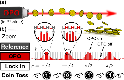
Here we present the use of a bi-stable configuration implemented in a period-doubling optical parametric oscillator for randomness generation. To the best of our knowledge, this is the first experimental utilization of a P2-state in an OPO reported in the literature to date. A simplified model is depicted in Fig. 1. The involved bi-stability is equi-energetic and equi-probable; only two outcomes are possible and no bias is observed. For randomness generation, the stream of binary outcomes can be used directly, and no additional un-biasing or bit-extraction is required. We test the outcome against the predicted outcomes of a fair coin toss. At the end of the paper, we compute the most conservative bound, the min-entropy, against the size of a finite sample of bits originating from the generator.
II Experimental Scheme
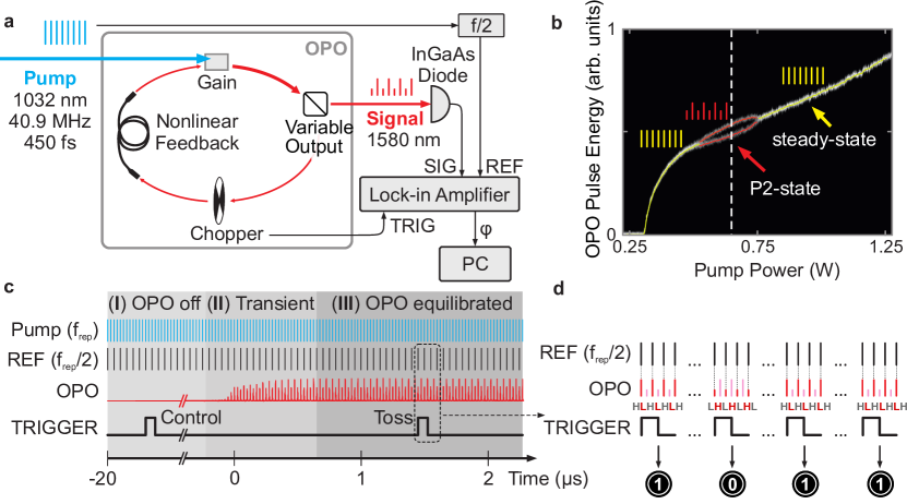
A home-built fiber-feedback optical parametric oscillator (OPO) Südmeyer et al. (2001); Steinle et al. (2015) is pumped by a mode-locked 450 fs, 1032 nm Yb:KGW oscillator (Fig. 2a). The gain element is a periodically poled lithium niobate crystal (PPLN). The repetition rate is defined by the laser and amounts to 40.9 MHz; the length of the OPO cavity is matched to this by a movable mirror. A part of the OPO cavity consists of a single-mode feedback fiber, which in combination with the variable output coupler allows to control the effective intracavity non-linearity. The output signal is detected on a reverse-biased InGaAs photo diode (Hamamatsu). The signal is monitored in real time on an oscilloscope (see Fig. 2c). Alternatively, the signal is fed into a lock-in amplifier for further analysis.
When the pump power is varied, the OPO exhibits a bi-modal behavior, which can be identified as period doubling Ikeda (1979); Lugiato et al. (1988); Richy et al. (1995); Steinmeyer et al. (1994); Kues et al. (2009). Above its oscillation threshold, the OPO operates in the steady-state (yellow trace in Fig. 2b), which results in an output pulse train with identical subsequent pulses, as known from any mode-locked laser. Upon further increase of pump power, the system enters the so-called period-2-state (P2-state) which delivers alternating pulses with different pulse energy, peak power, and spectral properties. This behavior originates from the interplay of spectral selective gain and nonlinear feedback Akhmediev et al. (2001). As a result of the synchronous pumping of the OPO, these pulses are temporally aligned with the pump frequency.
When the pump frequency (40.9 MHz in this case) is electronically divided by two, the pulse-train in the P2-state has a defined phase against this derived reference signal. When the OPO is turned on, this phase may be either in phase, or, with 50% probability, out of phase. This phase difference of can be unambiguously measured with various demodulation techniques. A simple and convenient way is the relative multiplication between the detected signal and the reference. A simple commercial solution is the detection with a lock-in amplifier, which allows for a direct access to the relative phase, . Here, a Zurich Instruments lock-in amplifier is used (UHFLI). The measurement time to determine the phase amounts to 1 s.
For random number generation, the OPO is turned on and off by an optical chopper, which is installed such that it can inhibit the cavity oscillation. Fig. 2c shows the sequence of generating one single bit in the generator: The measured signal (red) is measured versus the reference signal (REF), which corresponds to half of the repetition rate of the pump laser (). This measurement is performed twice in one chopper cycle: When the OPO is off – as the control signal – and when the OPO is in the P2-state – as the signal of the running oscillator, the tossed and landed coin. The control measurement is performed to verify that two subsequent measurements do not carry spurious information from one to the next outcome. A sequence of four consecutive measurements in the on-state is depicted in Fig. 2d. H and L denote the two alternating, high and low pulse energy outputs of the OPO in the P2-state, respectively.
The measurement outcome is saved by a Matlab (Matlab Inc.) script into a comprehensive set of data, which saves all measured phases. These can be either analyzed as direct phases, or alternatively processed as bit outcomes.
The measured phase of the oscillating OPO exhibits essentially two measurement outcomes: and . By means of a simple threshold the measurements are selected into a binary outcome. Values above zero phase are associated with the outcome , whereas values below zero are assigned a value of . Equally, these outcomes are the two possible stable configurations of the P2-state, () or (), where the order is fixed by the reference signal, at half of the pump frequency (see Fig. 2d). In the description above, a bold character denotes that the pulse from the OPO is not coinciding with the reference pulse train. This corresponds to a (red) colored character in Fig. 1 or 2. The measurement results were plotted in a histogram, and exhibit a very narrow distribution around the estimated value (see Fig. 3b).
III Origin of Randomness
It is well established in the literature that the randomness element in the transient process of a starting OPO originates from quantum effects. These include vacuum fluctuations in the gain element as well as cavity losses Herrero-Collantes and Garcia-Escartin (2017); Wang et al. (2013); Marandi et al. (2012b); Drummond et al. (2002); Nabors et al. (1990); Harris et al. (1967); Louisell et al. (1961). The primary quantum process in the build-up of the oscillation is the generation of single photons in a spontaneous down conversion process caused by pumping the non-linear gain crystal Marandi et al. (2012b); Louisell et al. (1961); Harris et al. (1967). The exact contribution of these processes to the formation of the P2-state is currently under investigation. In the context of randomness generation, it is important to note that the period doubling attractor is in particular not a chaotic attractor Uchida et al. (2008); Kanter et al. (2010). This is despite the fact that period doubling and chaos might occur in one and the same nonlinear system, as outlined in detail in the supplementary material ste .
The independence of the primary randomness process against small fluctuations of the pump power is a crucial feature. In order to demonstrate this peculiarity, we have performed numerical pulse propagation simulations (RP Pro Pulse from RP Photonics) of the transient process with an artificially fixed additional seed. These show that a relative intensity change of more than is required to induce a phase change by in the measured outcome. However, the measured relative intensity noise Steinle et al. (2016) integrated from 10 kHz to 20 MHz amounts to and is thus approximately a factor of too low to be the relevant driver of the randomness generation.
Moreover, the independence of subsequent measurement outcomes is important, as discussed on the observed bits below. Therefore, the inter-bit waiting time was reduced in an additional experiment by a factor of 1000. This was performed with the OPO operated in an extended cavity configuration, such that four independent pulses oscillate simultaneously in the cavity. A subsequent measurement reads four bits within a single chopper cycle. This reduces the relevant timescale for the comparison of successive bits from 100 s to 100 ns and thus eliminates the contribution of mechanical vibrations, chopper jitter, thermal effects, and pump intensity noise. Nevertheless, we measure alternating bits, which would not be the case if any of the above technical effects would cause the randomness (see supplementary material ste ). These investigations indicate that quantum effects are a significant source of randomness in our system.
In order to further quantify the randomness this process produces, we analyze the measured phase and its binary representation for a large set of outcomes in the next section.
IV From raw-bits to final bits
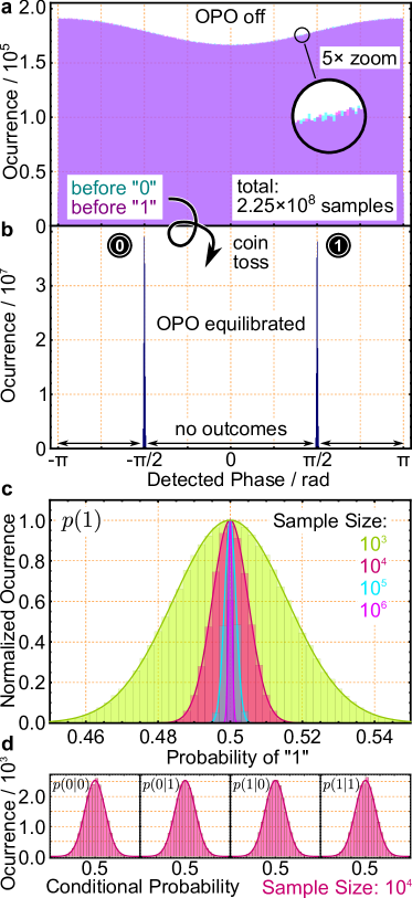
The first analysis of the acquired data involves the measured phase of the OPO in its off state. Fig. 3a shows a histogram of the raw phase output of the lock-in, right before each measurement of the running OPO. The data itself is divided into outcomes preceding an outcome of , and outcomes preceding an outcome of . Evidently, both datasets are very similar, and do not show any particular preference for subsequent outcomes. The small bias (wavy curve) is based on spurious signals reaching the lock-in amplifier and is symmetric for both phase outcomes.
After the transient time has passed, a second measurement determines the final state (=OPO on). As above, this is analyzed by the lock-in amplifier, resulting in a histogram of events. Both possible outcomes are centered around and , respectively. Their distribution is determined by experimental uncertainty to determine the phase. This results from spurious phase information, spontaneous down-conversion in the crystal, the sampling and measurement time, and residual (phase) noise in the signal. The width of the determined outcomes () amounts to 0.0023 rad. In other words, the outcomes are separated by more than 400 standard deviations – excluding the possibility that the two outcomes are confused. Such ambiguity-free measurements cannot be achieved in generators which are based on photon counting due to e.g. dark counts Stefanov et al. (2000); Svozil (2009); Oberreiter and Gerhardt (2016).
In the course of approximately one day a number of 22.25108 measurements were performed. We now analyze a possible bias or imbalance of the experimental outcomes, caused for example by technical noise Mitchell et al. (2015). This noise would produce additional measurement outcomes, which in information theoretical terms add up to the randomness in the transient process of the generator. For the analysis, the bit stream is divided into sub-strings of length and the experimental probability of the outcome is determined. The distribution is centered around 0.5, independently of the sample size . The analysis reconfirms the width of the distribution as . Please note that the data is not fitted but the theoretical curve is depicted along with the measured data.
The balance of the measurement outcomes is only one indication of a well balanced coin toss. Another important measure is the conditional probability which signifies whether subsequent outcomes contain some form of memory of the prior state of the oscillator. For this, a first indication is given by the analysis of Fig. 3a and b – still, this does not prove the independence of the outcomes of subsequent measurements in the equilibrated OPO. The conditional probability of obtaining the result after a preceding result is denoted as , reading as the probability of one conditioned on zero. This is defined as , and is depicted in Fig. 3c, along with the theoretical prediction of its distribution . An auto-correlation analysis, which also accounts for higher order bit-to-bit correlations is given in the supplementary material ste . Again, the expected behavior is reconfirmed and no memory in the system is evident.
Very common is the use of so-called random number tests. The tests ent, the NIST test suite Rukhin et al. (2010), the die-harder suite, or the most comprehensive TestU01 suite L’Ecuyer and Simard (2007) are commonly known. Many people still believe that such tests are able to show whether a bit-string is random or not. But they can only deliver the proof that no substantial flaw occurred in the implementation of a random bit generator. Moreover, most of these tests are based on algorithmic information theory and are designed to test algorithmically generated pseudo-random numbers rather than random numbers generated by physical processes Calude (2010). Therefore, the statement that a certain bit-string passes all tests does not prove the random nature of the input. Non-random and predictable numbers, such as the binary expansion of , pass all these tests flawlessly. As expected, our presented generator passes all these tests, and a sample output for the NIST suite is presented in the supplementary material ste .
A subset of the described random number tests is the analysis of different bit-patterns and their occurrence in the data set. This approach has been examined in early discussions on random number testing Knuth (1968). Nowadays, other authors suggest the use of information theoretic language for random number testing Calude (2010). In this context the coin tossing constants by W. Feller, which are closely related to the generalized Fibonacci numbers Finkelstein and Whitley (1978), describe the asymptotic probability of the event that a sequence with the length of or does not occur in a sequence of tosses of a fair coin. Feller’s constants have the property
| (1) |
The given Table 1 displays the analysis of sub-strings of length 400 bits of the generator. This small number is chosen to have non-vanishing values for the probabilities associated with higher order parameters (). The experimentally determined value is given in the third column, and the relative deviation of the order of 10-4 corresponds to the square root (=shot noise) of 2.25108 recorded bits. The computed values of the coin tossing constants match very well to the assumed behavior of the supplied random bit sequence.
The coin tossing constants analyze higher orders of tuples than the conditional probability and are therefore similar in this respect to a mathematical Borel-normality test Knuth (1968), which analyzes the lexicographical occurrence of all possible binary strings. Such a test was implemented by C. Calude for testing a number of (hardware-based) randomness generators Calude et al. (2010).
The above analysis on the probability of subsequent sets of measurement outcomes underlines the behavior of an ideal coin toss. An interesting effect occurs when we process the measurement outcomes by pairing each bit with exactly one neighboring bit, without allowing any overlaps of the tuples – unlike as before. Although we find all tuple permutations (, , , ) to be equally probable, the waiting time, which is the “distance” between two equivalent outcomes is different between the bit-changing (, ) and bit-equivalent outcomes (, ). For the tuples including a bit-flip, the predicted waiting time is 4 consecutive tosses. On the other hand a double sequence of , or , has a predicted waiting time of 6 consecutive tosses. This is verified with the present set of data and we determine values of 3.99976 and 5.99784 respectively. Again, the relative uncertainty of approximately corresponds to the length of the data-set; it proves that there is no further memory storage in the measurement outcomes and reconfirms the predicted behavior.
In summary, we conclude that the measured raw bits of the presented all-optical randomness generator using a nonlinear feedback OPO in the P2-state do not differ by any measurable means from the ones of a perfect Bernoulli trial. This is indicated by the independence of consecutive measurement outcomes, the balance between the two probabilities, and further tests, which resemble the expected outcomes of a perfect coin toss. Subsequently, the required post-processing can be reduced to a minimum. Such a post-processing would generally be required for any physical implementation of a fair (perfect) coin-toss due to finite size effects. We now turn to the entropy analysis of the raw-bit stream.
| Relative change | |||
|---|---|---|---|
| 2 | 1.23606798 | – | – |
| 3 | 1.08737803 | – | – |
| 4 | 1.03758013 | 1.03676354 | 7.8701073510-4 |
| 5 | 1.01732078 | 1.01731406 | 6.6112577510-6 |
| 6 | 1.00827652 | 1.00827933 | -2.7887701310-6 |
| 7 | 1.00403411 | 1.00403701 | -2.8845978010-6 |
| 8 | 1.00198836 | 1.00198588 | 2.4736371510-6 |
| 9 | 1.00098624 | 1.00098584 | 4.0111750110-7 |
| 10 | 1.00049092 | 1.00049182 | -8.9935776910-7 |
| 11 | 1.00024486 | 1.00024624 | -1.3815274410-6 |
| 12 | 1.00012226 | 1.00012358 | -1.3144145610-6 |
| 13 | 1.00006109 | 1.00006163 | -5.4041673610-7 |
| 14 | 1.00003053 | 1.00003025 | 2.7998685610-7 |
| 15 | 1.00001526 | 1.00001522 | 4.3391655010-8 |
V Entropy estimation
While all above measures suggest that the raw-bits are usable as a perfect source of random bits, we have ignored an important information theoretical measure of the output of the experimental apparatus so far: The generated entropy. As outlined below, the crucial quality figure for a randomness generator is the achievable entropy per output bit. Ideally, each bit has the perfect entropy of unity, which means that each generated bit can be used as an independent optical coin-toss and resembles the output of a fair coin. But when a finite fraction of bits is analyzed, this can only be proven if all s and s are equally balanced. Intrinsically, there might be an unwanted (but statistically allowed!) bias. In this case the determined entropy will be lower than one. Due to the finite length, this is most likely the case for the presented data-set. A first naive approach to calculate the entropy analyzes the balance of the bit-stream, and is given by the unconditional Shannon entropy which is defined as
| (2) |
Where is the single probability of obtaining or in the full bit sequence, respectively. This, however, does not consider any dependence or memory effects in the measurement outcomes, where for example an alternating sequence …would result in the same entropy as a fully random, i.e. totally unordered sequence. Therefore, the conditional entropy is considered, accounting for the memory (or the absence thereof) in the system. This is defined as
| (3) | |||||
We refer to the supplemental material ste for details of our calculation of the conditional entropy, but mention for clarity that the events y and x are defined as “the -th bit is ()” and “the -th bit is ()”. Uppercase Y and X are the unified sets of events on all bits. Thus, our notion of entropy is linked to the frequency analysis of output data, but can also be estimated a priori. Unlike the Shannon entropy, the min-entropy (denoted as ) is the most conservative bound for the usable entropy of a randomness generator. It maximizes the (conditional) probability against . This imbalance and maximizing effect can be seen in Fig. 3c and d. It becomes evident, that for a larger sample size , the width of the distribution shrinks and the amount of entropy is commonly larger. The min-entropy is defined as
| (4) |
The above entropy definitions can be straight-forwardly computed for an experimentally generated data-set. This will result in a scalar entropy value, which still has to be interpreted; for a good generator the resulting number will be usually close to one. How “perfect” the entropy is and how close it reaches to one, depends on three factors: a) the quality of the generator, b) the size of the analyzed bit stream (here denoted as for the number of analyzed bits), and, c) which particular data set is analyzed. Conclusively, it is very unlikely to achieve an entropy of unity when the entropy for a finite bit string is computed. This even holds for a fair coin. In the following, we perform an analysis of the generator’s outcome and compute if the entropy matches the predicted value.
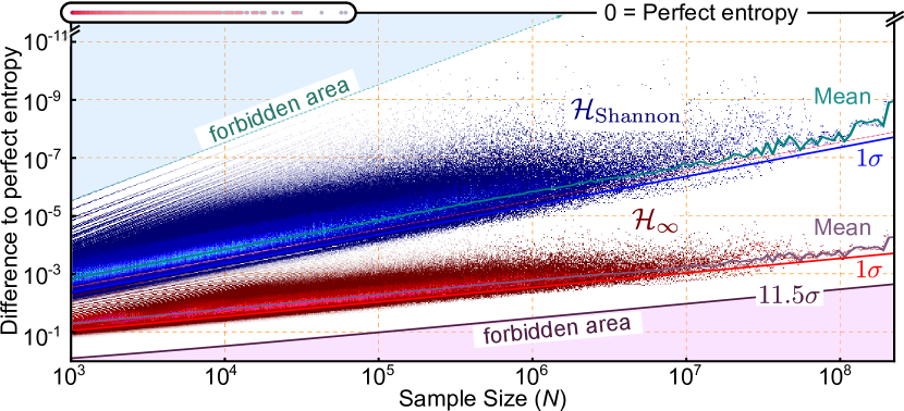
Fig. 4 shows the calculated Shannon and min-entropy for the presented data-set against the sample size, . To note that this graph shows the deviation against perfect entropy on a logarithmic scale. For a smaller sample size (left-hand side), a larger number of samples exist, and more points are depicted. As mentioned before, with a larger sample size, , the entropy approaches unity. The conditional Shannon-entropy scales linearly with , whereas the min-entropy is proportional to . The value and the distribution of the min-entropy is significantly smaller than for the Shannon-entropy, since the conditional probability is maximized. Fig. 4 also shows entropy bounds which are obtained a priori. These include the second highest possible value of the entropy for a certain sample size, besides the ideal case of perfect entropy. This is the highest value which can occur, when a minimally entropy-changing single bit-flip is present in a dataset of length . These curves scale quadratic against the mean slope behavior which was introduced above. Therefore, the mean value for the conditional Shannon-entropy forms a parallel line to the highest min-entropy, where one bit-flip is present.
The min-entropy is a conservative bound and selects the maximal conditional probability in a set of random bits. If a perfect random string is infinitely long, every possible occurrence will show up in a subset of this sequence. Then, in contradiction to the description above, a set of calculated entropies would eventually be very small since a very long sequence of seemingly non-random bits can occur (e.g. such as …). For these cases, the calculated entropy may be reduced to zero. For realistic considerations it is therefore important to exclude for instance such infinitesimally likely events of all bits of a long sequence being . Such a calculation of the occurrence of a certain set of equivalent outcomes of a generator was presented in the calculation of the coin tossing constants above (Table 1). Additionally, a possible error bound for randomness extraction was introduced by M. Troyer and R. Renner Troyer and Renner (2012) as . Such bounds are also described to guarantee an “-randomness” Mitchell et al. (2015). The proposed bound of ensures that one million generators do not have the option to exhibit the same outcome (i.e. a so-called collision of two generators) in the age of the universe. In the case of Gaussian distributed events this corresponds to approximately 11.5 standard deviations from the center of the distribution. Fig. 4 shows this bound as the lowest curve, obtained a priori by an error propagation on the entropy of a fair coin as outlined in the supplementary material ste . As suggested from the raw bit analysis, no selected sub-set of the bits falls below this line – this suggests that the model of a perfect coin toss seems to be appropriate for the introduced generator.
For our presented sample size of 2.25108 the conditional min-entropy per bit can be estimated as 99.95%. This can be simply read from Fig. 4 on the right hand side. This is, of course, solely limited by the finite sample volume. The most conservative bound (11.5 ) of the entropy difference to unity is approximately one order of magnitude different, and the entropy amounts to 99.5%.
With the raw bits, as discussed above, but also by merit of the calculated entropies, we are able to prove that the recorded bit-stream does not differ by any measurable means from a perfect coin toss. Each emitted bit can therefore be used as a random bit. No further randomness extraction has to be considered, when a large enough bit string is used. Of course, we are only able to prove this assumption bound to the size of the recorded bit string.
VI Conclusion & Outlook
An unbiased all-optical coin toss has been presented. It is based on the bi-stable outcome of an optical parametric oscillator with nonlinear fiber feedback, operating in the P2-state. The detection scheme relies on phase detection versus an external reference pulse. This implementation is substantially simpler than prior published experiments Marandi et al. (2012b, a); Okawachi et al. (2016), since it does not require degenerate operation of the OPO. The disadvantage of degenerate operation is that it necessitates either an actively interferometrically stabilized resonator to fix the relative optical phases of the signal and idler frequency combs to the pump frequency comb, or a “shaker” using a “dither and lock” algorithm that periodically varies the cavity length to generate an error signal for the stabilization. This introduces noise to the system which can be avoided by a non-degenerate operation.
The implemented detection scheme, based on period doubling, is ambiguity free, i.e. has only two possible outcomes, separated by more than 400 standard deviations, which can be interpreted as zeros and ones of a random bit sequence. This uniquely decouples the fundamental randomness process from the detection principle. While the detection here is based on a lock-in amplifier, more simple schemes can be developed. A demodulator or a radio-frequency mixer and a comparator will reduce the implementation costs, and emit the random sequence directly into an e.g. TTL level output.
One limitation is given by the sample rate of the chopper, which is limited to 10 kHz in the presented design. This sample rate is ultimately limited by the transient process until the OPO is in a stable state and the required time for phase detection. The measurement time to determine the phase amounts to 1 s with the current detection system. This may be shortened in future experiments by a factor of 10. Accordingly, a faster chopper can be installed as well. As evident in Fig. 2c, we estimate the time for equilibration to approximately 300 ns and the ambiguity-free detection of the phase state to two to three cycles, amounting to 100-150 ns. With the described OPO, and by introducing a faster chopper, a random bit rate above 1 MHz can be reached. An even further speed-up can be implemented with a higher repetition rate of the pump laser. For such changes, OPOs reaching the GHz range are reported Roth et al. (2004). As a side-effect, this would result in a much more compact design for the entire experimental configuration. Building a more compact randomness generator could further be realized by implementing the introduced principle with state-of-the-art technology on a photonic chip Niehusmann et al. (2004); Kuyken et al. (2013); Abellan et al. (2016).
The full quantum mechanical description of the open quantum system, specifically in the P2-state, remains to be addressed in future work. Commonly, the process of a bi-stable outcome of an OPO is described as a quantum process Herrero-Collantes and Garcia-Escartin (2017); Wang et al. (2013); Marandi et al. (2012b); Drummond et al. (2002); Nabors et al. (1990); Harris et al. (1967); Louisell et al. (1961), growing from quantum mechanical vacuum fluctuations. A careful analysis on the transient process, which may also introduce a fiber-optic electro-optic modulator instead of a chopper, along with more research on the power dependence will likely characterize this process and the P2-state in further detail. A deeper understanding of the underlying physics might lead to faster phase detection and larger random bit rates, and even to future implementations in quantum information processing and quantum simulation Inagaki et al. (2016).
Acknowledgements.
We acknowledge the support for the 3D-rendering by Ingmar Jakobi for Fig. 1. We further acknowledge the funding from the MPG, the SFB project CO.CO.MAT/TR21, ERC (Complexplas), the BMBF, the Eisele Foundation, the project Q.COM, and SMel.References
- Galton (1890) Francis Galton. Dice for statistical experiments. Nature, 42:13–4, 1890. URL http://dx.doi.org/10.1038/042013a0.
- Lenstra et al. (2012) Arjen K. Lenstra, James P. Hughes, Maxime Augier, Joppe W. Bos, Thorsten Kleinjung, and Christophe Wachter. Ron was wrong, Whit is right. IACR, 2012. http://eprint.iacr.org/.
- Becker et al. (2013) Georg T Becker, Francesco Regazzoni, Christof Paar, and Wayne P Burleson. Stealthy dopant-level hardware trojans. In International Workshop on Cryptographic Hardware and Embedded Systems, pages 197–214. Springer, 2013.
- Knuth (1968) Donald Knuth. The Art of Computer Programming - Volume 2 - Seminumerical Algorithms. Addison-Wesley, 1968. URL http://en.wikipedia.org/wiki/The_Art_of_Computer_Programming.
- Bauke and Mertens (2004) Heiko Bauke and Stephan Mertens. Pseudo random coins show more heads than tails. Journal of Statistical Physics, 114(3):1149–1169, 02 2004. ISSN 0022-4715. URL http://dx.doi.org/10.1023/B:JOSS.0000012521.67853.9a.
- Feller (1968) William Feller. An Introduction to Probability Theory and Its Applications. Wiley, 3rd edition, 1968.
- Murray and Teare (1993) Daniel B. Murray and Scott W. Teare. Probability of a tossed coin landing on edge. Phys. Rev. E, 48:2547–2552, Oct 1993. doi: 10.1103/PhysRevE.48.2547. URL http://link.aps.org/doi/10.1103/PhysRevE.48.2547.
- Finkelstein and Whitley (1978) Mark Finkelstein and Robert Whitley. Fibonacci numbers in coin tossing sequences. Fibonacci Quarterly, 16(6), 1978. URL http://escholarship.org/uc/item/9nx172g1.
- Ford (1983) Joseph Ford. How random is a coin toss. Physics Today, 36(4):40–47, 1983. URL http://dx.doi.org/10.1063/1.2915570.
- Vulović and Prange (1986) Vladimir Z. Vulović and Richard E. Prange. Randomness of a true coin toss. Phys. Rev. A, 33:576–582, Jan 1986. doi: 10.1103/PhysRevA.33.576. URL http://link.aps.org/doi/10.1103/PhysRevA.33.576.
- Stipčević (2004) Mario Stipčević. Fast nondeterministic random bit generator based on weakly correlated physical events. Review of Scientific Instruments, 75(11):4442–4449, 2004. doi: 10.1063/1.1809295. URL http://dx.doi.org/10.1063/1.1809295.
- Stefanov et al. (2000) André Stefanov, Nicolas Gisin, Olivier Guinnard, Laurent Guinnard, and Hugo Zbinden. Optical quantum random number generator. Journal of Modern Optics, 47(4):595–598, 2000. doi: 10.1080/09500340008233380. URL http://dx.doi.org/10.1080/09500340008233380.
- Jennewein et al. (2000) Thomas Jennewein, Ulrich Achleitner, Gregor Weihs, Harald Weinfurter, and Anton Zeilinger. A fast and compact quantum random number generator. Review of Scientific Instruments, 71(4):1675–1680, 2000. doi: 10.1063/1.1150518. URL http://link.aip.org/link/?RSI/71/1675/1.
- Stipčević and Rogina (2007) M. Stipčević and B. Medved Rogina. Quantum random number generator based on photonic emission in semiconductors. Review of Scientific Instruments, 78(4):045104, 2007. doi: 10.1063/1.2720728. URL http://link.aip.org/link/?RSI/78/045104/1.
- Fürst et al. (2010) Martin Fürst, Henning Weier, Sebastian Nauerth, Davide G. Marangon, Christian Kurtsiefer, and Harald Weinfurter. High speed optical quantum random number generation. Opt. Express, 18(12):13029–13037, Jun 2010. doi: 10.1364/OE.18.013029. URL http://www.opticsexpress.org/abstract.cfm?URI=oe-18-12-13029.
- Colbeck (2009) Roger Colbeck. Quantum And Relativistic Protocols For Secure Multi-Party Computation. PhD thesis, University of Cambridge, 2009.
- Pironio et al. (2010) S. Pironio, A. Acin, S. Massar, A. Boyer de la Giroday, D. N. Matsukevich, P. Maunz, S. Olmschenk, D. Hayes, L. Luo, T. A. Manning, and C. Monroe. Random numbers certified by bell’s theorem. Nature, 464(7291):1021–1024, April 2010. ISSN 0028-0836. URL http://dx.doi.org/10.1038/nature09008.
- Sanguinetti et al. (2014) Bruno Sanguinetti, Anthony Martin, Hugo Zbinden, and Nicolas Gisin. Quantum random number generation on a mobile phone. Phys. Rev. X, 4:031056, Sep 2014. doi: 10.1103/PhysRevX.4.031056. URL http://link.aps.org/doi/10.1103/PhysRevX.4.031056.
- Jofre et al. (2011) M. Jofre, M. Curty, F. Steinlechner, G. Anzolin, J. P. Torres, M. W. Mitchell, and V. Pruneri. True random numbers from amplified quantum vacuum. Optics Express, 19(21):20665–20672, Oct 2011. ISSN 1094-4087. URL https://www.osapublishing.org/abstract.cfm?uri=oe-19-21-20665.
- Marandi et al. (2012a) Alireza Marandi, Nick C. Leindecker, Vladimir Pervak, Robert L. Byer, and Konstantin L. Vodopyanov. Coherence properties of a broadband femtosecond mid-IR optical parametric oscillator operating at degeneracy. Optics Express, 20(7):7255–7262, March 2012a. ISSN 1094-4087. URL https://doi.org/10.1364/OE.20.007255.
- Okawachi et al. (2016) Yoshitomo Okawachi, Mengjie Yu, Kevin Luke, Daniel O. Carvalho, Michal Lipson, and Alexander L. Gaeta. Quantum random number generator using a microresonator-based kerr oscillator. Opt. Lett., 41(18):4194–4197, Sep 2016. doi: 10.1364/OL.41.004194. URL http://ol.osa.org/abstract.cfm?URI=ol-41-18-4194.
- Marandi et al. (2012b) Alireza Marandi, Nick C. Leindecker, Konstantin L. Vodopyanov, and Robert L. Byer. All-optical quantum random bit generation from intrinsically binary phase of parametric oscillators. Optics Express, 20:19322–19330, 2012b. URL https://doi.org/10.1364/OE.20.019322.
- Herrero-Collantes and Garcia-Escartin (2017) Miguel Herrero-Collantes and Juan Carlos Garcia-Escartin. Quantum random number generators. Rev. Mod. Phys., 89:015004, Feb 2017. doi: 10.1103/RevModPhys.89.015004. URL https://link.aps.org/doi/10.1103/RevModPhys.89.015004.
- Wang et al. (2013) Zhe Wang, Alireza Marandi, Kai Wen, Robert L. Byer, and Yoshihisa Yamamoto. Coherent Ising machine based on degenerate optical parametric oscillators. Physical Review A, 88(6):063853, December 2013. doi: 10.1103/PhysRevA.88.063853. URL https://link.aps.org/doi/10.1103/PhysRevA.88.063853.
- Drummond et al. (2002) P. D. Drummond, K. Dechoum, and S. Chaturvedi. Critical quantum fluctuations in the degenerate parametric oscillator. Physical Review A, 65(3):033806, February 2002. doi: 10.1103/PhysRevA.65.033806. URL https://link.aps.org/doi/10.1103/PhysRevA.65.033806.
- Nabors et al. (1990) C. D. Nabors, S. T. Yang, T. Day, and R. L. Byer. Coherence properties of a doubly resonant monolithic optical parametric oscillator. JOSA B, 7(5):815–820, May 1990. ISSN 1520-8540. doi: 10.1364/JOSAB.7.000815. URL https://www.osapublishing.org/abstract.cfm?uri=josab-7-5-815.
- Harris et al. (1967) S. E. Harris, M. K. Oshman, and R. L. Byer. Observation of Tunable Optical Parametric Fluorescence. Physical Review Letters, 18(18):732–734, May 1967. doi: 10.1103/PhysRevLett.18.732. URL https://link.aps.org/doi/10.1103/PhysRevLett.18.732.
- Louisell et al. (1961) W. H. Louisell, A. Yariv, and A. E. Siegman. Quantum Fluctuations and Noise in Parametric Processes. I. Physical Review, 124(6):1646–1654, December 1961. doi: 10.1103/PhysRev.124.1646. URL https://link.aps.org/doi/10.1103/PhysRev.124.1646.
- Oberreiter and Gerhardt (2016) Lukas Oberreiter and Ilja Gerhardt. Light on a beam splitter: More randomness with single photons. Laser & Photonics Reviews, 10(1):108–115, January 2016. ISSN 1863-8899. doi: 10.1002/lpor.201500165. URL http://dx.doi.org/10.1002/lpor.201500165.
- Südmeyer et al. (2001) T. Südmeyer, J. Aus der Au, R. Paschotta, U. Keller, P. G. R. Smith, G. W. Ross, and D. C. Hanna. Femtosecond fiber-feedback optical parametric oscillator. Opt. Lett., 26(5):304–306, Mar 2001. doi: 10.1364/OL.26.000304. URL http://ol.osa.org/abstract.cfm?URI=ol-26-5-304.
- Steinle et al. (2015) T. Steinle, F. Neubrech, A. Steinmann, X. Yin, and H. Giessen. Mid-infrared fourier-transform spectroscopy with a high-brilliance tunable laser source: investigating sample areas down to 5 m diameter. Opt. Express, 23(9):11105–11113, May 2015. doi: 10.1364/OE.23.011105. URL http://www.opticsexpress.org/abstract.cfm?URI=oe-23-9-11105.
- Ikeda (1979) Kensuke Ikeda. Multiple-valued stationary state and its instability of the transmitted light by a ring cavity system. Optics Communications, 30(2):257 – 261, 1979. ISSN 0030-4018. doi: http://dx.doi.org/10.1016/0030-4018(79)90090-7. URL //www.sciencedirect.com/science/article/pii/0030401879900907.
- Lugiato et al. (1988) LA Lugiato, C Oldano, C Fabre, E Giacobino, and RJ Horowicz. Bistability, self-pulsing and chaos in optical parametric oscillators. Il Nuovo Cimento D, 10(8):959–977, 1988. URL http://dx.doi.org/10.1007/BF02450197.
- Richy et al. (1995) C Richy, KI Petsas, E Giacobino, C Fabre, and L Lugiato. Observation of bistability and delayed bifurcation in a triply resonant optical parametric oscillator. JOSA B, 12(3):456–461, 1995. URL https://doi.org/10.1364/JOSAB.12.000456.
- Steinmeyer et al. (1994) G. Steinmeyer, D. Jaspert, and F. Mitschke. Observation of a period-doubling sequence in a nonlinear optical fiber ring cavity near zero dispersion. Optics Communications, 104(4):379 – 384, 1994. ISSN 0030-4018. doi: http://dx.doi.org/10.1016/0030-4018(94)90574-6. URL http://www.sciencedirect.com/science/article/pii/0030401894905746.
- Kues et al. (2009) Michael Kues, Nicoletta Brauckmann, Till Walbaum, Petra Groß, and Carsten Fallnich. Nonlinear dynamics of femtosecond supercontinuum generation with feedback. Opt. Express, 17(18):15827–15841, Aug 2009. doi: 10.1364/OE.17.015827. URL http://www.opticsexpress.org/abstract.cfm?URI=oe-17-18-15827.
- Akhmediev et al. (2001) N. Akhmediev, J. M. Soto-Crespo, and G. Town. Pulsating solitons, chaotic solitons, period doubling, and pulse coexistence in mode-locked lasers: Complex ginzburg-landau equation approach. Phys. Rev. E, 63:056602, Apr 2001. doi: 10.1103/PhysRevE.63.056602. URL https://link.aps.org/doi/10.1103/PhysRevE.63.056602.
- Uchida et al. (2008) Atsushi Uchida, Kazuya Amano, Masaki Inoue, Kunihito Hirano, Sunao Naito, Hiroyuki Someya, Isao Oowada, Takayuki Kurashige, Masaru Shiki, Shigeru Yoshimori, Kazuyuki Yoshimura, and Peter Davis. Fast physical random bit generation with chaotic semiconductor lasers. Nature Photonics, 2(12):728–732, December 2008. ISSN 1749-4885. doi: 10.1038/nphoton.2008.227. URL https://www.nature.com/nphoton/journal/v2/n12/full/nphoton.2008.227.html.
- Kanter et al. (2010) Ido Kanter, Yaara Aviad, Igor Reidler, Elad Cohen, and Michael Rosenbluh. An optical ultrafast random bit generator. Nat Photon, 4(1):58–61, January 2010. ISSN 1749-4885. URL http://dx.doi.org/10.1038/nphoton.2009.235.
- (40) See Supplemental Material for details on the experimental setup, additional randomness measures, the entropy calculation, and the in-depth calculation of Feller’s coin tossing constants. URL http://link.aps.org/supplemental/10.1103/PhysRevX.7.041050.
- Steinle et al. (2016) Tobias Steinle, Florian Mörz, Andy Steinmann, and Harald Giessen. Ultra-stable high average power femtosecond laser system tunable from 1.33 to 20 m. Optics Letters, 41(21):4863–4866, November 2016. ISSN 1539-4794. doi: 10.1364/OL.41.004863. URL https://www.osapublishing.org/abstract.cfm?uri=ol-41-21-4863.
- Svozil (2009) Karl Svozil. Three criteria for quantum random-number generators based on beam splitters. Phys. Rev. A, 79(5):054306, May 2009. URL http://link.aps.org/doi/10.1103/PhysRevA.79.054306.
- Mitchell et al. (2015) Morgan W. Mitchell, Carlos Abellan, and Waldimar Amaya. Strong experimental guarantees in ultrafast quantum random number generation. Phys. Rev. A, 91:012314, Jan 2015. doi: 10.1103/PhysRevA.91.012314. URL https://link.aps.org/doi/10.1103/PhysRevA.91.012314.
- Rukhin et al. (2010) Andrew Rukhin, Juan Soto, James Nechvatal, Miles Smid, Elaine Barker, Stefan Leigh, Mark Levenson, Mark Vangel, David Banks, Alan Heckert, James Dray, and San Vo. A statistical test suite for random and pseudorandom number generators for cryptographic applications. NIST Report, 2010.
- L’Ecuyer and Simard (2007) Pierre L’Ecuyer and Richard Simard. Testu01: A C library for empirical testing of random number generators. ACM Transactions on Mathematical Software, 33(4):1–40, August 2007. URL http://www.iro.umontreal.ca/~lecuyer/myftp/papers/testu01.pdf.
- Calude (2010) Cristian S. Calude. Information and Randomness: An Algorithmic Perspective. Springer, 2nd ed. edition, December 2010. ISBN 9783642077937.
- Calude et al. (2010) Cristian S. Calude, Michael J. Dinneen, Monica Dumitrescu, and Karl Svozil. Experimental evidence of quantum randomness incomputability. Physical Review A, 82(2):022102, August 2010. URL http://dx.doi.org/10.1103/PhysRevA.82.022102.
- Troyer and Renner (2012) M. Troyer and R. Renner. A randomness extractor for the quantis device. Internal Report, pages 1–7, 2012. URL http://marketing.idquantique.com/acton/attachment/11868/f-004d/1/-/-/-/-/quantis-rndextract-techpaper.pdf.
- Roth et al. (2004) J. M. Roth, T. G. Ulmer, N. W. Spellmeyer, S. Constantine, and M. E. Grein. Wavelength-tunable 40-ghz picosecond harmonically mode-locked fiber laser source. IEEE Photonics Technology Letters, 16(9):2009–2011, Sept 2004. ISSN 1041-1135. doi: 10.1109/LPT.2004.833036. URL http://dx.doi.org/10.1109/LPT.2004.833036.
- Niehusmann et al. (2004) Jan Niehusmann, Andreas Vörckel, Peter Haring Bolivar, Thorsten Wahlbrink, Wolfgang Henschel, and Heinrich Kurz. Ultrahigh-quality-factor silicon-on-insulator microring resonator. Opt. Lett., 29(24):2861–2863, Dec 2004. doi: 10.1364/OL.29.002861. URL http://ol.osa.org/abstract.cfm?URI=ol-29-24-2861.
- Kuyken et al. (2013) Bart Kuyken, Xiaoping Liu, Richard M. Osgood, Roel Baets, Günther Roelkens, and William M. J. Green. A silicon-based widely tunable short-wave infrared optical parametric oscillator. Opt. Express, 21(5):5931–5940, Mar 2013. doi: 10.1364/OE.21.005931. URL http://www.opticsexpress.org/abstract.cfm?URI=oe-21-5-5931.
- Abellan et al. (2016) Carlos Abellan, Waldimar Amaya, David Domenech, Pascual Mu noz, Jose Capmany, Stefano Longhi, Morgan W. Mitchell, and Valerio Pruneri. Quantum entropy source on an inp photonic integrated circuit for random number generation. Optica, 3(9):989–994, Sep 2016. doi: 10.1364/OPTICA.3.000989. URL http://www.osapublishing.org/optica/abstract.cfm?URI=optica-3-9-989.
- Inagaki et al. (2016) Takahiro Inagaki, Yoshitaka Haribara, Koji Igarashi, Tomohiro Sonobe, Shuhei Tamate, Toshimori Honjo, Alireza Marandi, Peter L. McMahon, Takeshi Umeki, Koji Enbutsu, Osamu Tadanaga, Hirokazu Takenouchi, Kazuyuki Aihara, Ken-ichi Kawarabayashi, Kyo Inoue, Shoko Utsunomiya, and Hiroki Takesue. A coherent ising machine for 2000-node optimization problems. Science, 2016. ISSN 0036-8075. doi: 10.1126/science.aah4243. URL http://science.sciencemag.org/content/early/2016/10/19/science.aah4243.