Approximations in the homogeneous Ising model

Abstract

The Ising model is important in statistical modeling and inference in many applications, however its normalizing constant, mean number of active vertices and mean spin interaction – quantities needed in inference – are computationally intractable. We provide accurate approximations that make it possible to numerically calculate these quantities in the homogeneous case. Simulation studies indicate good performance of our approximation formulae that are scalable and unfazed by the size (number of nodes, degree of graph) of the Markov Random Field. The practical import of our approximation formulae is illustrated in performing Bayesian inference in a functional Magnetic Resonance Imaging activation detection experiment, and also in likelihood ratio testing for anisotropy in the spatial patterns of yearly increases in pistachio tree yields.

I Introduction

Let $\boldsymbol{X}=\{X_{1},\ldots,X_{n}\}$ be $n$ binary random variables with a conditional graph dependence structure specified via the neighborhood ${\mathcal{N}}=\{(i,j):i\!\sim\!j,1\leq i<j\leq\ n\}$, where the notation $i\!\sim\!j$ indicates existence of an edge between the $i$th and $j$th nodes in the graph. The celebrated Ising model of statistical physics specifies the joint probability mass function (PMF)

$$\begin{split}\mathbb{P}(\boldsymbol{X}=\boldsymbol{x};\boldsymbol{\alpha},\boldsymbol{\beta})\propto\exp\bigl{[}\sum_{i}\alpha_{i}x_{i}+\sum_{i\sim j}\beta_{ij}\bigl{\{}x_{i}x_{j}+(1-x_{i})(1-x_{j})\bigr{\}}\bigr{]},\end{split}$$ (1)

where it is assumed that $x_{i}\in\{0,1\}\,\forall i=1,2,\ldots,n$, $\boldsymbol{x}=(x_{1},\ldots,x_{n})$, $\boldsymbol{\alpha}=(\alpha_{1},\ldots,\alpha_{n})$ and $\boldsymbol{\beta}=(\beta_{ij};1\leq i<j\leq\ n)$. The parameter $\alpha_{i}\geq 0$ modulates the chance that $X_{i}\!=\!1$ while the parameter $\beta_{ij}$ specifies the strength of the interaction between $X_{i}$ and $X_{j}$ when $i\!\sim\!j$. The PMF (1) has summation constant or partition function denoted by $Z(\boldsymbol{\alpha},\boldsymbol{\beta})$.

Model (1) was proposed by [1] to his student Ernst Ising as a way to characterize magnetic phase transitions or singularities in the partition function over a lattice graph. [2] published the model that bears his name and showed that in one dimension, that is, for a linear lattice graph, the phase transition structure is trivial with no singularities in the partition function. The distribution has applicability in disciplines beyond physics – indeed, one of its earliest uses in the statistical literature was as a prior model for a binary scene in image analysis [3]. Other applications include state-time disease surveillance [4, 5] and mapping [6, 7, 8]; modeling of protein hydrophobicity [9], genetic codon bias thermodynamics [10], DNA elasticity [11] or ion channel interaction [12] in statistical genetics; modeling of electrophysiological phenomena of the retina [13] and cortical recordings in neuroscience [14, 15, 16]; and modeling of biological evolution [17]. The Ising model has also been used to model voting patterns of senators in the US Congress [18] or behaviors on social networks [19, 20]. While many of these applications use a regular lattice structure, some (e.g. [18, 19, 20]) use more general non-lattice structures.

Parameter estimation in the Ising model is often challenging, especially in the context of multi-dimensional lattices, and more generally for non-lattice conditional dependence graphs. This difficulty flows from the computational impracticality of obtaining exact closed-form expressions for the partition function in the presence of $\beta_{ij}$s. Indeed, the computation of $Z(\boldsymbol{\alpha},\boldsymbol{\beta})$ in such graphs with an external field has been shown to be NP-complete [21]. Even though the partition function is just a finite sum of exponential functions and can consequently be analytically expressed so that there is no phase transition for the finite graph Ising model, its computation is still intractable. Nevertheless, parameter estimation is needed in many applications, as in the two illustrative examples of Section IV. In some cases, parameter estimation has been eschewed in favor of approaches that are not always wholly satisfactory but obviate the need for its estimation. For example, [7] would ideally have liked to have estimated the interaction parameter for assessing Medicare service area boundaries for competing hospice systems in Duluth, Minnesota, but they instead fixed the value for their study. Some authors have used empirical techniques such as pseudolikelihood (e.g.,[3, 19, 20]), or written (1) in terms of an exponential family model and then used moment-matching or maximum entropy methods [22, 14, 15, 16]. Yet others [23, 11, 9, 12, 10] have used simpler models, typically restricting to first order interactions, in order to employ a recursive algorithm to estimate the partition function [24] which is possible only with an Ising model with only nearest-neighbor (NN) structure (equivalently, first-order interactions). [25] used (1) in one dimension and with first-order neighborhood to signal if a probe (gene) is enriched or not, and specifically mentioned that they did not model more complex interactions because of the intractability of the partition function. Thus, there is need for a general method for estimating the partition function in several applications. Many methods have been suggested to estimate the normalizing constant of intractable PMFs and densities. Some authors (e.g. [26, 27, 28]) provided exact formulae for $Z(\boldsymbol{\alpha},\boldsymbol{\beta})$ in a 2D planar graph that also mostly assume a null $\boldsymbol{\alpha}$ in (1). These calculations also grow with the size of a graph and are not particularly useful for situations (e.g., Bayesian inference) where the partition function needs repeated evaluation. The popular method of path sampling [29, 30, 31] writes the normalizing constant as a function of the integral of an expectation, that is estimated by Monte Carlo or Markov Chain Monte Carlo (MCMC) sampling. Further, path sampling is usually implemented as a preprocessing step by evaluating $Z(\boldsymbol{\alpha},\boldsymbol{\beta})$ on a grid of parameter values.

Numerous other stochastic approaches (for a sampling, consider [32, 33, 34, 35, 36, 37, 38, 39, 40, 41, 42, 43, 44, 45]) exist, but they all come with major drawbacks beyond their need for long sampling periods in both burn-in and post-burn-in phases, that can be computationally demanding and are not scalable to larger problems. Further, these stochastic approaches can only estimate the partition function or moments at a discrete grid of parameter values, with interpolation (of unclear accuracy) needed for intermediate values, since these values are needed in a continuum, for instance, in the case of maximum likelihood parameter estimation and inference. In this paper, we therefore provide numerical approximations for the partition function, the mean number of active modes, and the mean spin interaction of the Ising model. Section II provides these approximation formulae separately for the isotropic (i.e., for when $\alpha_{i}\equiv\alpha$ and $\beta_{ij}\equiv\beta$ for $1\leq i\neq j\leq n$) and anisotropic cases. Our approximations yield formulae with computational expense unaffeced by the size (number of nodes, graph degree) of the Ising model, and therefore, unlike those obtained from stochastic methods, essentially infinitely scalable. Section III evaluates the accuracy of these approximation formulae. Section IV illustrates the utility and performance of these approximations in the context of Bayesian and likelihood-based inference. The paper concludes with some discussion. A supplement, with sections and equations prefixed by “S” is also available.

II Approximations in large Ising models

II-A The isotropic case

Our starting point is (1) under the assumptions of homogeneity and isotopy. Since $x_{j}x_{i}{+}(1{-}x_{i})(1{-}x_{j})=1{-}(x_{i}{-}x_{j})^{2}$, the isotropic homogeneous Ising model can be written as

$$\mathbb{P}(\boldsymbol{x};\alpha,\beta){=}Z(\alpha,\beta)^{-1}\exp\{\alpha\displaystyle\sum_{i=1}^{n}x_{i}{-}\beta\displaystyle\sum_{i\sim j}(x_{i}-x_{j})^{2}\},$$ (2)

where we write $Z(\boldsymbol{\alpha},\boldsymbol{\beta})$ as $Z(\alpha,\beta)$ to reflect that $\boldsymbol{\alpha}$ and $\boldsymbol{\beta}$ can be characterized by scalars $\alpha$ and $\beta$ in the isotropic homogenous context being considered here.

II-A1 The normalizing constant

Let $G_{n,m}=(V,E)$ be the graph underlying the data, where $m$ denotes the number of edges in the graph. The set of nodes is $V=\{x_{1},\ldots,x_{n}\}$ and the set of edges is $E=\{(x_{i},x_{j}):i\sim j\}$. Since each $x_{i}$ is either 0 or 1, we get the equivalent relation

$$\sum_{i\sim j}(x_{i}-x_{j})^{2}=\displaystyle\sum_{i=1}^{n}k_{i}x_{i}-2\displaystyle\sum_{i\sim j}x_{i}x_{j},$$

where $k_{i}$ is the degree of the $i$th node, that is, the number of edges linked to the node $i$, for $i=1,\ldots,n$. This article assumes a regular $G_{n,m}$ (see Ch. 3 of [46]), that is, $k_{i}=k$ for all nodes. The exponent in $\mathbb{P}(\boldsymbol{x};\alpha,\beta)$ is then $\alpha^{\prime}\displaystyle\sum_{i=1}^{n}x_{i}+\beta\displaystyle\sum_{i,j}\eta_{ij}x_{i}x_{j},$ where $\alpha^{\prime}=\alpha-k\beta$ and $\eta_{ij}=\mathbb{I}(i\sim j)$, with $\mathbb{I}(\cdot)$ the indicator function. Let $M(\ell)$ be the set of sequences $\boldsymbol{x}$ with $\displaystyle\sum_{i=1}^{n}x_{i}=\ell$. Then

$$\begin{split}Z(\alpha,\beta)=1&+\exp{(\alpha^{\prime}n+\beta kn)}+n\exp(\alpha^{\prime})+\displaystyle\sum_{\ell=2}^{n-1}\exp(\alpha^{\prime}\ell)\displaystyle\sum_{X\in M(\ell)}\exp\bigl{(}\beta\displaystyle\sum_{i,j}\eta_{ij}x_{i}x_{j}\bigr{)}.\end{split}$$ (3)

With a graph $G_{n,m}$ having a total of $m=nk/2$ edges and for a fixed $\ell$, only $\ell$ observations, say $\tilde{\boldsymbol{X}}_{\ell}=\{x_{i_{1}},x_{i_{2}},\ldots,x_{i_{\ell}}\}$, contribute to $\displaystyle\sum_{i,j}\eta_{ij}x_{i}x_{j}$, so that $\displaystyle\sum_{i,j}\eta_{ij}x_{i}x_{j}=\displaystyle\sum_{h=1}^{\ell}\displaystyle\sum_{j}\eta_{i_{h},j}x_{j}$. The set $\tilde{\boldsymbol{X}}_{\ell}$ can be thought of as a subgraph of the original graph, namely $G_{\ell}=(\tilde{\boldsymbol{X}}_{\ell},\tilde{E}_{\ell}),$ where the set of edges is a subset of all possible $\ell_{2}=\ell(\ell-1)/2$ edges between nodes in $\tilde{\boldsymbol{X}}_{\ell}$ that are present in $G_{n,m}$. In graph theory, the subgraphs $G_{\ell}$ are referred to as node-induced subgraphs. The node $x_{t}$ contributes to the sum $\displaystyle\sum_{h=1}^{\ell}\displaystyle\sum_{j}\eta_{i_{h},j}x_{j}$ only if $x_{t}$ is a node of $G_{\ell}.$ This sum corresponds to twice the number of edges in $G_{\ell}$. Computing the last sum in (3) corresponds to counting the number of subgraphs $G_{\ell}$ with a given number of edges. Our partition function approximation uses

Proposition 1.

Let $Y(s,\ell)$ be the number of node-induced subgraphs $G_{\ell}$ containing exactly $s$ edges. Then

$$Z(\alpha,\beta)=1+\exp{(\alpha^{\prime}n+\beta kn)}+n\exp(\alpha^{\prime})+\displaystyle\sum_{\ell=2}^{n-1}\binom{n}{\ell}\exp(\alpha^{\prime}\ell){\cal M}_{p(\cdot|\ell)}(2\beta),$$ (4)

where ${\cal M}_{p(\cdot|\ell)}(2\beta)$ is the moment generating function (MGF) associated with the distribution $p(s|\ell)=Y(s,\ell)/\binom{n}{\ell},$ $s\in\{0,1,\ldots,\ell k/2\},$ evaluated at $t=2\beta.$

Proof.

Write the last sum in (3) as

$$\begin{split}\displaystyle\sum_{X\in M(\ell)}\exp\bigl{(}\beta\displaystyle\sum_{i,j}\eta_{ij}x_{i}x_{j}\bigr{)}=\displaystyle\sum_{s=0}^{\ell_{2}}Y(s,\ell)\exp\bigl{(}2\beta s\bigr{)}=\binom{n}{\ell}\displaystyle\sum_{s=0}^{\ell_{2}}\exp\bigl{(}2\beta s\bigr{)}\,\tfrac{Y(s,\ell)}{\binom{n}{\ell}}.\end{split}$$

Conditional of $M(\ell)$, the proportions $Y(s,\ell)/\binom{n}{\ell}$ define a distribution on $s$. Because we suppose that the graph $G_{n,m}$ is regular, the support of $p(s|\ell)$ is over $\{0,1,\ldots,\ell k/2\}$. ∎

The number of edges, $s$, present in a given node-induced subgraph is half the sum of the degrees associated with the nodes present in the subgraph. Since as shown below the sum of degrees is the sum of several sums, we can approximate the distribution of $s$ given $M(\ell)$ for large $\ell$ via a normal distribution, and replace ${\cal M}_{p(\cdot|\ell)}(\cdot)$ by the Gaussian MGF. We formalize this approach further next.

For a given graph $G_{n,m}$, and $s$, $p(s|\ell)$ corresponds to the proportion of node-induced subgraphs with $\ell$ nodes and exactly $s$ edges between the nodes. Unfortunately, calculating $p(s|\ell)$ is not straightforward. So, instead of the number of edges $s$, we consider the degree distribution of the subgraphs. Let $r_{\ell,h}=\displaystyle\sum_{j=1}^{n}\eta_{i_{h},j}x_{j}$, for $h=1,2,\ldots,\ell.$ These quantities are the observed degrees of the nodes $x_{i_{1}},\ldots,x_{i_{\ell}}$. Let $r_{\ell}=\displaystyle\sum_{h=1}^{\ell}r_{\ell,h}$. The quantities $r_{\ell,h}$ and $r_{\ell}$ are realizations from the distribution of the degrees of the graph. In particular, finding their first two moments is enough as they fully characterize the normal distribution. The distribution of the number of node-induced subgraphs with degrees adding up to $r_{\ell}$ has the form

$$p_{d}(r_{\ell}|\ell)=\displaystyle\sum_{r_{\ell,1}+r_{\ell,2}+\cdots r_{\ell,\ell}=r_{\ell}}p(r_{\ell,1},r_{\ell,2},\ldots,r_{\ell,\ell}).$$

The support of this distribution lies over the even numbers $r_{\ell}=2s$. Also, the joint PMF $p(r_{\ell,1},r_{\ell,2},\ldots,r_{\ell,\ell})$ is not straightforward to compute. However, the marginals are easily obtained for a regular graph with $k$ edges for each node. In this case, $r_{\ell,h}$, the proportion of edges for a given node $x_{i_{h}}$ in a subgraph of $\ell$ nodes, has the hypergeometric distribution with parameters $(n-1,k,\ell-1)$. Therefore, the expectation of twice the number of edges is given by $\mu_{\ell}=E(r_{\ell})=\ell E(r_{\ell,h})=\ell(\ell-1)k/(n-1)=2\ell_{2}\theta,$ where $\theta=m/{n\choose 2}=k/(n-1)$ is the proportion of edges with respect to a complete graph. The variance depends on the dependency between the $r_{\ell,h}$s. Proceeding, we have the following

Proposition 2.

Let $\sigma_{\ell}^{2}=2\ell_{2}\theta(1-\theta)(1-\tfrac{\ell-2}{n-2})$, and $\rho_{\ell}=(\ell-1)(n-2k)/\{(n-2)(n-k-1)\}.$ We have $\operatorname{Var}(r_{\ell})=\sigma_{\ell}^{2}\bigl{(}1-\rho_{\ell}\bigr{)},$ and $\operatorname{Cov}(r_{\ell,t},r_{\ell,h})=-\sigma_{\ell}^{2}\rho_{\ell}/(2\ell_{2})={\cal O}(n^{-1}).$ In particular, for all $\ell=o(n)$, $\operatorname{Var}(r_{\ell})/\sigma_{\ell}^{2}\rightarrow 1$ as $n\rightarrow\infty$, or equivalently $\rho_{\ell}\rightarrow 0$ as $n\rightarrow\infty$, uniformly on $\ell=o(n)$.

Proof.

We have $\operatorname{Var}(\sum_{h=1}^{\ell}r_{\ell,h}){=}\sum_{h=1}^{\ell}(\ell-1)\theta(1-\theta)(1-y_{\ell,2})+2\sum_{t<h}\operatorname{Cov}(r_{\ell,t},r_{\ell,h})=\sigma_{\ell}^{2}+2\sum_{t<h}\operatorname{Cov}(r_{\ell,t},r_{\ell,h}),$ with $y_{\ell,2}=(\ell-2)/(n-2)$, and $\sigma_{\ell}^{2}=2\ell_{2}\theta(1-\theta)(1-y_{\ell,2}).$ Let $k_{th}$ be the number of neighbors in common between vertices $t$ and $h$. In the notation that follows, the conditional expectation given $\eta$, means that the values of the couples $(t,h)$ are fixed. Further,

$$\operatorname{Cov}(r_{\ell,t},r_{\ell,h}|\eta)=\displaystyle\sum_{i=1}^{n}\displaystyle\sum_{j=1}^{n}\eta_{hi}\eta_{tj}\operatorname{Cov}(x_{i},x_{j})\\ =\tfrac{1}{(n-1)^{2}}\biggl{\{}\displaystyle\sum_{i=1}^{n}\eta_{hi}\eta_{ti}{(\ell-1)(n-\ell)}-2\displaystyle\sum_{i<j}\eta_{hi}\eta_{tj}\tfrac{(\ell-1)(n-\ell)}{n-2}\biggr{\}}\\ =\tfrac{(\ell-1)(n-\ell)}{(n-1)^{2}}\biggl{(}\displaystyle\sum_{i=1}^{n}\eta_{hi}\eta_{ti}-{2}\displaystyle\sum_{i<j}\tfrac{\eta_{hi}\eta_{tj}}{n-2}\biggr{)}$$

Note that $E(k_{th}){=}nk(k{-}1)/\{(n{-}1)(n{-}2)\}{=}n\theta(k{-}1)/(n{-}2).$ Therefore

$$\operatorname{Cov}(r_{\ell,t},r_{\ell,h})=-\tfrac{(\ell-1)(n-\ell)(n-2k)}{(n-1)(n-2)^{2}}\theta.$$ (5)

These covariances tend to zero uniformly on $\ell{=}o(n)$ as $n{\rightarrow}+\infty$. For the variance, we have

$$\operatorname{Var}(r_{\ell})=\sigma_{\ell}^{2}\left\{1-\tfrac{(\ell-1)(n-2k)}{(n-2)(n-k-1)}\right\},$$

from where the proposition follows. ∎

Let $s_{\bullet}=\max(0,k-n+\ell)\,\ell/2$, $s^{\bullet}=\min(\ell-1,k)\,\ell/2$ and $\sigma_{\rho,\ell}=\sigma_{l}\sqrt{1-\rho_{\ell}}$. Set $w(\ell,s)=2\ell_{2}\{(s+\tfrac{1}{2})/\ell_{2}-\nu_{\ell}\}/\sigma_{\rho,\ell}$, where $\nu_{\ell}=\theta+\beta\sigma_{\rho,\ell}^{2}$. Let $\Phi(\cdot)$ denote the standard normal cumulative distribution function (CDF), and set $\Delta_{\Phi}(\ell)=\Phi(w(\ell,s^{\bullet}+\tfrac{1}{2}))-\Phi(w(\ell,s_{\bullet}-\tfrac{1}{2})).$ The above observations lead us to the following fact that backgrounds the main result of this section.

Fact.

The MGF ${\cal M}_{p_{d}(\cdot|\ell)}(2\beta)$ is well-approximated by $\exp\{2\beta\ell_{2}\theta+\tfrac{\beta^{2}}{2}\sigma^{2}_{\rho,\ell}\}\Delta_{\Phi}(\ell)$. Therefore the main bulk of the sum in (4) is well approximated by

$$\sum_{\ell\gg 1}^{o(n)}\binom{n}{\ell}\exp(\alpha^{\prime}\ell)\exp\{2\beta\ell_{2}\theta+\beta^{2}\ell_{2}\theta(1-y_{\ell,2})(1-\theta)(1-\rho_{\ell})\}\Delta_{\Phi}(\ell).$$

In fact, it is well known that the hypergeometric distribution is well approximated by a normal distribution provided that its variance goes to infinity (see p. 158, Section 4.4 of [47]). In our case, this means that the result is valid when $\ell=o(n)$. Also Hoeffding’s inequality (see Section 6 of [48]) for hypergeometric variables, states that each $r_{\ell,h}$ is concentrated about its mean $\mu_{\ell,1}=(\ell-1)\theta$, when $n$ is large and $\ell$ is moderate to large. So we just need to study the distribution about its mean. These results imply that the variables $r_{\ell,h}$ are well-approximated by, and behave like, normally distributed random variables with mean $\mu_{\ell,1}$, and variance $\sigma_{\ell,1}^{2}\approx\sigma_{\ell}^{2}/\ell$, for values of $\ell=o(n)$. Moreover, from Proposition 2, these Gaussian variables are nearly independent. Therefore their sum is also well-approximated by a normal random variable. That is, for large $\ell=o(n)$, we have

$$\begin{split}{\cal M}_{p_{d}(\cdot|\ell)}(2\beta)\approx\int_{2s_{\bullet}-1}^{2s^{\bullet}+1}\tfrac{1}{\sigma_{\rho,\ell}}\phi\biggl{(}\tfrac{x-\mu_{\ell}}{\sigma_{\rho,\ell}}\biggr{)}\exp(\beta x)dx,\end{split}$$ (6)

where $\phi(\cdot)$ stands for the standard normal density. A straightforward calculation simplifies (6) to

$$\exp\left(2\beta\theta\ell_{2}+\tfrac{\beta^{2}}{2}\sigma_{\rho,\ell}^{2}\right)\Delta_{\Phi}(\ell),$$

which is the desired result.

We propose an estimator of the partition function using the above results. To avoid the approximation at the extreme values of $\ell$, set $A_{\phi}(\alpha,\beta)=1+\exp(\alpha^{\prime}n+\beta kn)+n\exp(\alpha^{\prime})$. Also, let

$$g(\ell)=\alpha^{\prime}\ell+2\beta\theta\ell_{2}\{1+(\beta/2)\left(1{-}\tfrac{\ell-2}{n-2}\right)(1{-}\theta)(1{-}\rho_{\ell})\}$$

and define $\Sigma(\alpha,\beta){=}\displaystyle\sum_{\ell=2}^{n-1}\binom{n}{\ell}\exp\{g(\ell)\}\Delta_{\Phi}(\ell).$ Our partition function estimate $Z_{\phi}(\alpha,\beta)$, which we refer to as the normal-edge partition function estimate is

$$\begin{split}Z_{\phi}(\alpha,\beta)=&A_{\phi}(\alpha,\beta)+\Sigma(\alpha,\beta).\end{split}$$ (7)

The estimate $Z_{\phi}(\alpha,\beta)$ may be computed in ${\cal O}(n)$ operations. Although, this calculation is fast, we investigate a further approximation by replacing the summation in the last term of (7) by an integral. Specifically, we regard the summation as a Riemann sum, and hence, as an approximation to the corresponding integral. The integral can be calculated as a new summation with number of terms much smaller than $n$, yielding a final approximation that can be computed much faster than ${\cal O}(n)$. In fact, the Euler-MacLaurin formula [49] gives us the approximation

$$\Sigma(\alpha,\beta)\approx\int_{2}^{n-1}\tfrac{\Gamma(n+1)}{\Gamma(x)\Gamma(n-x)}\exp\{g(x)\}\Delta_{\Phi}(x)\,dx+B_{\phi}(\alpha,\beta),$$

where $2B_{\phi}(\alpha,\beta)=n\exp\{g(n-1)\}\Delta_{\Phi}(n-1)+{n\choose 2}\exp\{g(2)\}\Delta_{\Phi}(2).$ Using [50]’s approximation for the Gamma function, and writing $y=x/n=\ell/n$, in the above integral, we have $\Sigma(\alpha,\beta)\approx B_{\phi}(\alpha,\beta)+J_{n,k,\frac{1}{2}}(\alpha^{\prime},\,\beta),$ where, for every $t\in\mathbb{R}$, we have the function

$$J_{n,k,t}(\alpha,\,\beta)=\sqrt{\tfrac{n}{2\pi}}\int_{2/n}^{1-1/n}\tfrac{\Delta_{\Phi}(ny)\exp\{g(ny)\}}{(1-y)^{n(1-y)+\frac{1}{2}}y^{ny+t}}dy.$$ (8)

We denote this integral approximation to $Z_{\phi}(\alpha,\beta)$ by $\tilde{Z}_{\phi}(\alpha,\beta)$.

This integral approximation error is of order $\max_{y}|e(y)|/n$ where $e(y)$ is the derivative of the integrand in (8) and is equal to $\exp\{h(y)+g(y)\}(\Delta_{\Phi}(ny)(h^{\prime}(y)+g^{\prime}(y))+\Delta_{\Phi}^{\prime}(ny))$ with $h(y)=-[n(1-y)+\tfrac{1}{2}]\log(1-y)-(ny+\tfrac{1}{2})\log(y)$. This means that the relative error of the integral approximation is of order $n^{-1}$ because the terms in the summation are at most of the same order as $\max_{y}|e(y)|$.

II-A2 Moment approximations

Having found approximations for $Z(\alpha,\beta)$, we now approximate the first two moments of (1) under isotropy and homogeneity.

Mean number of active nodes

We first approximate $M{=}\mbox{I}\!\mbox{E}(\hat{M}){\equiv}\mbox{I}\!\mbox{E}(\sum_{i=1}^{n}x_{i})$, the expected number of active nodes. In addition to the setup in Section II-A1, let $\Delta_{\phi}(\ell)=\phi\{w(\ell,s^{\bullet}{+}\tfrac{1}{2})\}{-}\phi\{w(\ell,s_{\bullet}{-}\tfrac{1}{2})\}$. Define $C_{\phi.M}(\alpha,\beta)={n\choose 2}[\exp\{g(n{-}1)\}\Delta_{\Phi}(n{-}1){+}\exp\{g(2)\}\Delta_{\Phi}(2)].$ Using the same reasoning as before yields the following estimate for $M$:

$$\begin{split}M_{\phi}\doteq\tfrac{1}{{Z}_{\phi}}\biggl{\{}n\exp(\alpha^{\prime}n+\beta kn)+n\exp(\alpha^{\prime})+\displaystyle\sum_{\ell=2}^{n-1}\binom{n}{\ell}\ell\exp\{g(\ell)\}\Delta_{\Phi}(\ell)\biggr{\}}.\end{split}$$ (9)

Using [50]’s approximation, the Euler-MacLaurin expansion [49], and writing $\ell$ as $n(\ell/n)$, provides an approximation for the series in (9) as $C_{\phi.M}(\alpha,\beta){+}nJ_{n,k,-\frac{1}{2}}(\alpha,\,\beta)$, and thence

$$\begin{split}\tilde{M}_{\phi}=\tfrac{n}{\tilde{Z}_{\phi}}\bigl{\{}\exp{(\alpha^{\prime}n+\beta kn)}+\exp(\alpha^{\prime})+J_{n,k,-\frac{1}{2}}(\alpha,\beta)+C_{\phi.M}(\alpha,\beta)/n\bigr{\}}.\end{split}$$

Mean spin interaction

We now approximate the expected number of matches of the homogeneous isotropic Ising model, or its mean spin interaction $S=\mbox{I}\!\mbox{E}(\hat{S})=\mbox{I}\!\mbox{E}(\tfrac{1}{2}\sum_{i,j}\eta_{ij}x_{i}x_{j})$. Writing $Z{=}Z(\alpha,\beta)$, and proceeding as before,

$$\begin{split}S&=\tfrac{1}{Z}\displaystyle\sum_{\ell=0}^{n}\exp({\alpha^{\prime}\ell})\displaystyle\sum_{\boldsymbol{x}\in M(\ell)}\!\!\bigl{(}\tfrac{1}{2}\displaystyle\sum_{i,j}\eta_{ij}x_{i}x_{j}\bigr{)}\exp(\beta\displaystyle\sum_{i,j}\eta_{ij}x_{i}x_{j})\\ &=\tfrac{m}{Z}\exp({\alpha^{\prime}n+\beta kn})+\tfrac{1}{Z}\displaystyle\sum_{\ell=2}^{n-1}\binom{n}{\ell}\exp({\alpha^{\prime}\ell})\displaystyle\sum_{s=s_{\bullet}}^{s^{\bullet}}p(s|\ell)\,s\exp(2\beta s).\end{split}$$

From weak convergence arguments and similar reductions as in the approximation for the partition function $Z(\alpha,\beta)$, we get

$$\begin{split}\mbox{I}\!\mbox{E}\{\hat{S}\exp{(2\beta\hat{S})}\}&\approx\int_{2s_{\bullet}-1}^{2s^{\bullet}+1}\tfrac{1}{\sigma_{\rho,\ell}}\phi\biggl{(}\tfrac{x-\mu_{\ell}}{\sigma_{\rho,\ell}}\biggr{)}\tfrac{x}{2}\exp(\beta x)\,dx\\ &=\tfrac{1}{2}\tfrac{d}{d\beta}\int_{2s_{\bullet}-1}^{2s^{\bullet}+1}\tfrac{1}{\sigma_{\rho,\ell}}\phi\biggl{(}\tfrac{x-\mu_{\ell}}{\sigma_{\rho,\ell}}\biggr{)}\exp(\beta x)\,dx\\ &=\tfrac{1}{2}\exp\biggl{(}2\beta\theta\ell_{2}+\tfrac{\beta^{2}\sigma_{\rho,\ell}^{2}}{2}\biggr{)}\left\{(2\theta\ell_{2}+\beta\sigma_{\rho,\ell}^{2})\Delta_{\Phi}(\ell)-\sigma_{\rho,\ell}\Delta_{\phi}(\ell)\right\}.\end{split}$$

So we approximate $\mbox{I}\!\mbox{E}(\hat{S})$ as

$$S_{\phi}\doteq\tfrac{m}{Z_{\phi}}\exp(\alpha^{\prime}n+\beta kn)+\tfrac{1}{2Z_{\phi}}\displaystyle\sum_{\ell=2}^{n-1}\binom{n}{\ell}\biggl{[}\{2\theta\ell_{2}+\beta\sigma_{\rho,\ell}^{2}\}\Delta_{\Phi}(\ell)-\sigma_{\rho,\ell}\Delta_{\phi}(\ell)\biggr{]}\\ \qquad\times\exp\biggl{(}\alpha^{\prime}\ell+2\beta\theta\ell_{2}+\tfrac{\beta^{2}\sigma_{\rho,\ell}^{2}}{2}\biggr{)}.$$ (10)

Let $\zeta_{1}(\ell){=}1{+}\tfrac{\beta\sigma_{\rho,\ell}^{2}}{2\ell_{2}\theta}$, and $\zeta_{2}(\ell){=}\sigma_{\rho,\ell}\Delta_{\phi}(\ell)$. Define $D_{\phi.M}(\alpha,\beta)\doteq\tfrac{1}{2}\{\zeta_{1}(2)\Delta_{\Phi}(2)-\tfrac{n{-}1}{2k}\zeta_{2}(2)\}\exp\{g(2)\}+\{\tfrac{n-2}{2}\zeta_{1}(n-1)\Delta_{\Phi}(n{-}1){-}\tfrac{\zeta_{2}(n{-}1)}{2k}\}\exp\{g(n{-}1)\}.$ The expression in (10) can be further approximated as an integral in the same manner as before to obtain the approximation

$$\tilde{S}_{\phi}\doteq\tfrac{m}{\tilde{Z}_{\phi}}\biggl{[}\exp{(\alpha^{\prime}n+\beta kn)}+D_{\phi.M}(\alpha,\beta)\\ \qquad+\sqrt{\tfrac{n}{2\pi}}\int_{\tfrac{2}{n}}^{1-\tfrac{1}{n}}\biggl{\{}\zeta_{1}(ny)\Delta_{\Phi}(ny)-\tfrac{\zeta_{2}(ny)}{kny^{2}}\biggr{\}}\tfrac{\exp[\alpha^{\prime}ny+\tfrac{\beta kny^{2}}{2}\zeta_{1}(ny)]}{(1-y)^{n(1-y)+\frac{1}{2}}y^{ny-\frac{3}{2}}}\,dy\biggr{]},$$

upon replacing $kn/2$ by $m$, using [50]’s approximation to the binomial coefficients, and the Euler-MacLaurin approximation [49] for the sum.

II-B Extension to the anisotropic case

We now explore the case of the homogeneous anisotropic Ising model. We consider two sets of edges $E_{p},E_{v}$ induced by the neighborhood relations $E_{p}\!=\!\{(i,j):i\!\stackrel{{\scriptstyle\mbox{\scriptsize p}}}{{\sim}}\!j\}$, $E_{v}\!=\!\{(i,j):i\!\stackrel{{\scriptstyle\mbox{\scriptsize v}}}{{\sim}}\!j\}$, with $E_{p}\cap E_{v}=\emptyset$. For instance, we may think of $E_{p}$ as the set of edges in the same “plane” (or a 2D lattice) and of $E_{v}$ as the set of edges formed by two “planes” (of the third dimension in a 3D-lattice). Then the Ising model PMF is

$$\mathbb{P}(\boldsymbol{x};\alpha,\beta_{p},\beta_{v})=Z(\alpha,\beta_{p},\beta_{v})^{-1}\exp\left\{\alpha^{\prime\prime}\displaystyle\sum_{i=1}^{n}x_{i}+\beta_{p}\displaystyle\sum_{ij}\eta_{p,ij}x_{i}x_{j}+\beta_{v}\displaystyle\sum_{ij}\eta_{v,ij}x_{i}x_{j}\right\},$$ (11)

with $\alpha^{\prime\prime}=\alpha-\beta_{p}k_{p}-\beta_{v}k_{v},\eta_{p,ij}=\mathbb{I}(i\stackrel{{\scriptstyle\mbox{\scriptsize p}}}{{\sim}}j),\eta_{v,ij}=\mathbb{I}(i\stackrel{{\scriptstyle\mbox{\scriptsize v}}}{{\sim}}j)$, and where $k_{p}$ and $k_{v}$ are the degrees of the regular graphs $(V,E_{p})$ and $(V,E_{v})$. Proceeding similarly as before, $Z(\alpha,\beta_{p},\beta_{v})=1+\exp{(\alpha n)}+n\exp(\alpha^{\prime\prime})+\displaystyle\sum_{\ell=2}^{n-1}\!\!\exp(\alpha^{\prime\prime}\ell)\!\!\!\displaystyle\sum_{X\in M(\ell)}\!\!\!\exp\bigl{(}\beta_{p}\displaystyle\sum_{i,j}\eta_{p,ij}x_{i}x_{j}+\beta_{v}\displaystyle\sum_{i,j}\eta_{v,ij}x_{i}x_{j}\bigr{)}$. From identical arguments as in Proposition 1, we have

$$Z(\alpha,\beta_{p},\beta_{v})=A_{2}(\alpha,\beta_{p},\beta_{v})+\displaystyle\sum_{\ell=2}^{n-2}{n\choose\ell}\exp{(\alpha^{\prime\prime}\ell)}{\cal M}_{p(\cdot,\cdot|\ell)}(2\beta_{p},2\beta_{v}),$$

where $A_{2}(\alpha,\beta_{p},\beta_{v})=1+\exp{(\alpha n)}+n\exp{(\alpha^{\prime\prime})}+n\exp{\{\alpha(n-2)+\alpha^{\prime\prime}\}},$ and

$${\cal M}_{p(\cdot,\cdot|\ell)}(2\beta_{p},2\beta_{v})=\!\displaystyle\sum_{\mathclap{\begin{subarray}{c}s_{p},s_{v}=0\\ s_{p}+s_{v}\leq\ell_{2}\end{subarray}}}\exp\{2\beta_{p}s_{p}+2\beta_{v}s_{v}\}\tfrac{Y(s_{p},s_{v},\ell)}{{n\choose\ell}},$$

with $Y(s_{p},s_{v},\ell)$ equal to the number of node-induced graphs $G_{\ell}$ containing exactly $s_{p}$ edges in $E_{p}$ and exactly $s_{v}$ edges in $E_{v}$. As before, consider $r_{p,\ell,h}=\sum_{j=1}^{n}\eta_{p,i_{h},j}x_{j}$, and similarly, $r_{v,\ell,h}=\sum_{j=1}^{n}\eta_{v,i_{h},j}x_{j}$, where $\{x_{i_{1}},\ldots,x_{i_{\ell}}\}$ is the set of nodes of the graph $G_{\ell}$. Let $r_{p,\ell}{=}\sum_{h=1}^{\ell}r_{p,\ell,h}$, and $r_{v,\ell}{=}\sum_{h=1}^{\ell}r_{v,\ell,h}$. As in the derivation of $Z_{\phi}$ earlier, we argue that the joint PMF $p(r_{p,\ell},r_{v,\ell}\lvert\ell)$ behaves like a bivariate normal distribution, and hence ${\cal M}_{p(\cdot,\cdot|\ell)}(2\beta_{p},2\beta_{v})$ is approximately

$$\int_{2s_{p\bullet}-1}^{2s_{p}^{\bullet}+1}\int_{2s_{v\bullet}-1}^{\min(2s_{v}^{\bullet}+1,2s_{pv}^{\bullet}+1-x)}\tfrac{\exp(\beta_{p}x+\beta_{v}y)}{2\pi\sqrt{\operatorname{det}(V_{\ell})}}\exp\{{-}(x{-}\mu_{p,\ell},y{-}\mu_{v,\ell})V_{\ell}^{-1}(x{-}\mu_{p,\ell},y{-}\mu_{v,\ell})^{\prime}\}\,dxdy,$$ (12)

where $s_{a\bullet}=\max(0,k_{a}-n+\ell)\ell/2$, $s_{a}^{\bullet}=\min(\ell-1,k_{a})\ell/2$, for $a=p,v$, $s_{pv}^{\bullet}=\min(\ell_{2},(k_{p}+k_{v})\ell/2)$, $\mu_{p,\ell}=2\ell_{2}\theta_{p}$, and $\mu_{v,\ell}=2\ell_{2}\theta_{v}$, with $\theta_{p}=k_{p}/(n-1),$ and $\theta_{v}=k_{v}/(n-1)$; and

$$V_{\ell}=\begin{pmatrix}\sigma_{p,\ell}^{2}(1-\rho_{p,\ell})&\sigma_{p,v,\ell}\\ \sigma_{p,v,\ell}&\sigma_{v,\ell}^{2}(1-\rho_{v,\ell})\end{pmatrix}.$$

Let $\tau_{p,\ell}^{2}=\sigma_{p,\ell}^{2}(1-\rho_{p,\ell})$, and $\tau_{v,\ell}^{2}=\sigma_{v,\ell}^{2}(1-\rho_{v,\ell})$. A straightforward calculation shows that (12) reduces to

$$\exp\biggl{\{}\beta_{p}\mu_{p,\ell}+\beta_{v}\mu_{v,\ell}+\tfrac{1}{2}(\beta_{p},\beta_{v})V_{\ell}(\beta_{p},\beta_{v})^{\prime}\biggr{\}}\Delta_{\Phi_{2}}(\ell),$$

where $\Phi_{2}(\cdot)$ is the standard bivariate normal CDF, and $\Delta_{\Phi_{2}}(\ell)$ is $\Phi_{2}(\cdot)$ evaluated in the region $V_{\ell}^{-1/2}\bigl{[}\Omega_{1}-\{(\mu_{p,\ell},\mu_{v,\ell})^{\prime}+V_{\ell}(\beta_{p},\beta_{v})^{\prime}\}\bigr{]}$, with $\Omega_{1}=[2s_{p\bullet}-1,2s_{p}^{\bullet}+1]\times[2s_{v\bullet}-1,2s_{v}^{\bullet}+1]$. From here, approximation formulae analogous to the ones in (7) and (8) are readily obtained for the anisotropic case. For example, let $g_{2}(\ell)=\alpha^{\prime\prime}\ell+\beta_{p}\mu_{p,\ell}+\beta_{v}\mu_{v,\ell}+\tfrac{1}{2}(\beta_{p},\beta_{v})V_{\ell}(\beta_{p},\beta_{v})^{\prime}$, and $2B_{2,\phi}(\alpha,\beta_{p},\beta_{v})={n\choose 2}\exp\{g_{2}(n-2)\}\Delta_{\Phi_{2}}(n-2)+{n\choose 2}\exp\{g_{2}(2)\}\Delta_{\Phi_{2}}(2)$. We have the approximation

$$\begin{split}\tilde{Z}_{\phi}(\alpha,\beta_{p},\beta_{v})=&A_{2}(\alpha,\beta_{p},\beta_{v})+B_{2,\phi}(\alpha,\beta_{p},\beta_{v})\sqrt{\tfrac{n}{2\pi}}\int_{2/n}^{1-2/n}\tfrac{\Delta_{\Phi_{2}}(ny)\exp\{g_{2}(ny)\}}{(1-y)^{n(1-y)+\frac{1}{2}}y^{ny+\frac{1}{2}}}dy.\end{split}$$ (13)

Remark.

The variance-covariance $V_{\ell}$ is obtained in a similar manner as the variances and covariances in the single graph case. We have

$$\operatorname{Cov}(r_{p,\ell,t},r_{v,\ell,h}\lvert\eta)=\displaystyle\sum_{i=1}^{n}\displaystyle\sum_{j=1}^{n}\eta_{v,hi}\eta_{p,tj}\operatorname{Cov}(x_{i},x_{j})\\ =\tfrac{(\ell-1)(n-\ell)}{(n-1)^{2}}\left\{\displaystyle\sum_{i=1}^{n}\eta_{p,ti}\eta_{v,hi}-\tfrac{2}{n-2}\displaystyle\sum_{i<j}\eta_{v,hi}\eta_{p,tj}\right\}=2k_{p}k_{v}\tfrac{(\ell-1)(n-\ell)}{(n-1)^{2}(n-2)^{2}}.$$

Next we proceed as in Section II-A to obtain $M_{\phi}$, $\tilde{M}_{\phi}$, $S_{\phi}$ and $\tilde{S}_{\phi}$. However, now we need to estimate both $S_{p,\phi}$ and $S_{v,\phi}$. The estimates $M_{\phi},S_{p,\phi},S_{v,\phi}$ correspond to the derivatives of $\log Z_{\phi}(\alpha,\beta_{p},\beta_{v})$ with respect to $\alpha$, $\beta_{p}$, and $\beta_{v}$, respectively. The approximations based on integrals instead of summations can be seen to correspond to derivatives of $\log Z_{\tilde{\phi}}(\alpha,\beta_{p},\beta_{v})$ as well. Therefore, estimates of $\tilde{M}_{\phi}$, $\tilde{S}_{p,\phi}$ and $\tilde{S}_{v,\phi}$ can be obtained directly from derivatives of $Z_{\tilde{\phi}}(\alpha,\beta_{p},\beta_{v})$. For brevity, we sketch the ideas here, and refer to Section S1 for explicit approximations to $\mbox{I}\!\mbox{E}(M)$, $\mbox{I}\!\mbox{E}(S_{p})$ and $\mbox{I}\!\mbox{E}(S_{v})$.

III Performance evaluations

III-A Approximation formulae assessments

We evaluated performance of the analytical approximation formulae derived in Section II by comparing them with those obtained by simulation. The mean activation and spin interaction were estimated for a range of $(\alpha,\beta)$-pairs using MCMC – these estimates were assumed to be the “gold standard” for our comparisons. However, MCMC simulation-based estimation of $Z(\alpha,\beta)$ is very difficult, so we used path sampling [29, 30] to obtain its reference value. Our approximation formulae apply to any regular graph, but for convenience, we only evaluated performance on lattice graphs. (Because of edge effects, our lattice graphs are only approximately regular.) We note also that the use of MCMC methods here is simply to assess the accuracy of our formulae: while faster stochastic approaches may be resorted to, we consider it largely irrelevant in our comparisons, simply because it is inherently unfair to the stochastic methods to compare the performance of our approximation formulae that are completely scalable and near-immediately calculated, to any stochastic method, that generated the Ising model and is affected by its size. Therefore, the real evaluation of our method is in its accuracy. Also, because our approximation formulae rely on asymptotic reductions, it is of special interest to understand their accuracy in less favorable contexts where asymptotic arguments may be more suspect. Therefore, our evaluations are on moderate, but realistic-sized fields. We also reiterate that formulae rely on asymptotic reductions, and therefore it is of special interest to understand their accuracy in less favorable contexts where asymptotic arguments may be more suspect. We consider the isotropic and anistropic cases separately.

III-A1 The isotropic case

We simulated realizations from Ising models on two lattice configurations and with three different neighborhood orders. The two lattices had grids of sizes $116{\times}152$ and $64{\times}64$, respectively. The neighborhoods we chose for our simulations were of the first, second and fifth orders, corresponding to graphs of degree $k{=}4,8$ and $24$, respectively. For each of the six combinations of grid sizes and graph degrees, we compared performance for 1,102 different pairs of values of the Ising parameters $(\alpha,\beta){\in}[0,\,5]{\times}[0.005,\,10]$ (19 values for $\alpha$, and 58 values for $\beta$). Note that there is no need to evaluate the approximations for negative $\alpha$ because $Z(-\alpha,\beta){=}\exp{(-\alpha n)}Z(\alpha,\beta)$ for all pairs $(\alpha,\beta)$. (In particular, moments such as $\mbox{I}\!\mbox{E}_{-\alpha,\beta}(\hat{M})$ can be easily obtained from $\mbox{I}\!\mbox{E}_{\alpha,\beta}(\hat{M})$.) For each setting, we estimated the Ising moments and normalizing constant from samples obtained using the Swendsen-Wang [51] algorithm with a burn-in period of 10,000 iterations and a sample size of 10,000 realizations from the post-burn-in iterations and used these estimates as the “gold standard” reference values. For each moment estimate, we evaluated the performance of our approximations relative to the MCMC estimate by computing both the absolute value difference between the MCMC estimate ${m_{MC}}$ and the analytical approximation given by the Normal edge proportion approximation ${m_{N}}$, and the relative absolute difference between these quantities $|m_{MC}{-}m_{N}|/m_{MC}.$ The measures of absolute ($L_{1}$) and relative ($R_{1}$) discrepancy between all evaluations in the grid for $(\alpha,\beta)$ are given by the difference between the approximated and estimated surfaces

$$L_{1}(m_{MC},m_{N}){=}V^{-1}\int\int|m_{MC}(\alpha,\beta)-m_{N}(\alpha,\beta)|\,d\alpha\,d\beta,$$

and

$$R_{1}(m_{MC},m_{N}){=}V^{-1}\int\int\frac{|m_{MC}(\alpha,\beta)-m_{N}(\alpha,\beta)|}{|m_{MC}(\alpha,\beta)|}\,d\alpha\,d\beta,$$

with $V{=}\int\int d\alpha\,d\beta.$ We also show the ratio of the absolute discrepancy to the mean volume of the region below the surface, given by $m_{MC}$, $L_{1}(m_{MC},m_{N})/V_{MC}$, where $V_{MC}{=}(V^{-1}\int\int m_{MC}d\alpha\,d\beta)$. Table I shows the relative and absolute discrepancies between the analytical approximations of $\log Z(\alpha,\beta)$ and the path sampling estimates using the MCMC samples. The path sampling estimates were obtained using the estimate of the expected matches, that is $\log Z_{MC}(\alpha,\beta){=}\int_{0}^{\beta}\operatorname{Mean}_{\alpha,b}(\sum_{i\sim j}\delta_{ij}^{(t)})\,db+n\log\{1+\exp{(\alpha)}\}{-}m\beta,$ where $\delta_{ij}^{(t)}$ is the observed value of $\delta_{ij}$ in the $t$th sample generated by the Swendsen-Wang algorithm and, as before, $m$ is the number of edges in the graph.

TABLE I: Discrepancies associated with the approximation of the logarithm of the partition function. Here, we have two lattice grids ($\mathbb{G}$), A of size $116\!\times\!152$ and $B$ of size $64\times 64$ respectively, with regular graph of degree $k$. All discrepancies are computed against the MCMC path sampling estimates which forms our “gold standard” for comparisons in these experiments, except for the case $k{=}2$, whose discrepancies were computed using the known asymptotic formula for the 2-NN graph.

		Absolute and Relative Discrepancies
		$L_{1}$		$L_{1}/V_{MC}$		$R_{1}$
$\mathbb{G}$	$k$	$\tilde{Z}_{\phi}$	$Z_{\phi}$	$\tilde{Z}_{\phi}$	$Z_{\phi}$	$\tilde{Z}_{\phi}$	$Z_{\phi}$
A	$2$	$26.72$	$26.73$	$0.0006$	$0.0006$	$0.009$	$0.009$
A	$4$	$270.48$	$270.55$	$0.006$	$0.006$	$0.032$	$0.032$
A	$8$	$437.97$	$438.00$	$0.010$	$0.010$	$0.047$	$0.047$
A	$24$	$373.57$	$373.59$	$0.008$	$0.008$	$0.044$	$0.044$
B	$2$	$6.20$	$6.20$	$0.0006$	$0.0006$	$0.009$	$0.009$
B	$4$	$62.86$	$62.93$	$0.006$	$0.006$	$0.032$	$0.032$
B	$8$	$100.81$	$100.81$	$0.010$	$0.010$	$0.047$	$0.047$
B	$24$	$88.24$	$88.24$	$0.009$	$0.009$	$0.044$	$0.044$

Table I indicates that both the direct Normal edge proportion estimate and its counterpart that uses the Euler-MacLaurin formula perform similarly. Thus there is almost no loss in accuracy when using the faster Euler-MacLaurin based estimate. In order to further show the value of this simplified approximation, we also compared this analytical approximation with the theoretical asymptotic result for the logarithm of the normalizing constant for the 2-nearest-neighbor (2-NN) graph, that is, for $k{=}2$. Section S2-A shows that $\log Z(\alpha,\beta)$ approximately equals

$$\tfrac{n(\alpha-\beta)}{2}+n\log\biggl{[}\exp(\beta/2)\cosh(\alpha/2)+\sqrt{\exp(\beta)\cosh^{2}(\alpha/2)-2\sinh(\beta)}\biggr{]},$$ (14)

after adapting the result of  [52, Chapter 13, page 261] to the case of the {0,1}-statespace 2-NN Ising model. Performance evaluations for this case are also in Table I, with the results again indicating that the numerical approximation works very well even for the smallest possible value of $k$ even though these approximations are based on moderate to large values of $k$.

TABLE II: Absolute and relative discrepancies between MCMC estimates of (a) the mean number of active nodes or (b) the mean spin interaction, and their numerical approximations for lattice grids ($\mathbb{G}$) A of size $116\!\times\!152$ and B of size $64\!\times\!64$, and degree $k$.

		Absolute and Relative Discrepancies
		$L_{1}$		$L_{1}/V_{MC}$		$R_{1}$
$\mathbb{G}$	$k$	$\tilde{M}_{\phi}$	$M_{\phi}$	$\tilde{M}_{\phi}$	$M_{\phi}$	$\tilde{M}_{\phi}$	$M_{\phi}$
A	$4$	$18.94$	$19.71$	$0.001$	$0.001$	$0.002$	$0.002$
A	$8$	$8.42$	$8.81$	$0.0005$	$0.0005$	$0.0009$	$0.0009$
A	$24$	$2.84$	$2.94$	$0.0002$	$0.0002$	$0.0003$	$0.0003$
B	$4$	$4.14$	$4.32$	$0.001$	$0.001$	$0.002$	$0.002$
B	$8$	$0.73$	$0.74$	$0.0002$	$0.0002$	$0.0003$	$0.0003$
B	$24$	$0.25$	$0.25$	$0.00006$	$0.00006$	$0.0001$	$0.0001$

(a) Mean number of active nodes

		Absolute and Relative Discrepancies
		$L_{1}$		$L_{1}/V_{MC}$		$R_{1}$
$\mathbb{G}$	$k$	$\tilde{S}_{\phi}$	$S_{\phi}$	$\tilde{S}_{\phi}$	$S_{\phi}$	$\tilde{S}_{\phi}$	$S_{\phi}$
A	$4$	$39.18$	$41.47$	$0.001$	$0.001$	$0.002$	$0.002$
A	$8$	$33.57$	$35.90$	$0.0005$	$0.0005$	$0.0009$	$0.001$
A	$24$	$33.80$	$34.65$	$0.0002$	$0.0002$	$0.0003$	$0.0003$
B	$4$	$9.27$	$9.35$	$0.001$	$0.001$	$0.002$	$0.002$
B	$8$	$3.94$	$3.00$	$0.0003$	$0.0002$	$0.0004$	$0.0003$
B	$24$	$3.85$	$2.66$	$0.00008$	$0.00006$	$0.0001$	$0.0001$

(b) Mean spin interaction

Table II reports the values of the absolute value and relative discrepancies for the relevant moments (mean activation and spin interaction) of the Ising model. The results indicate good performance of our approximation formulae relative to the MCMC estimates. It is worth noting that the MCMC algorithm took about four days to compute the 1,102 sets of moments for each combination of grid-size and graph degree combination, while our approximation formula took well under a second for each calculation. (We stress that our approximations result in formulae, so that our computational cost is unaffected by larger-sized MRFs).

III-A2 The anisotropic model case

We also evaluated performance of the approximation formulae derived in Section II-B.

TABLE III: Mean relative discrepancies between MCMC estimates and numerical approximations for the anisotropic case (standard deviations are shown within parentheses). The simulations are made on a lattice of dimension $66{\times}106$ to match the setting of the pistachios datasets.

Relative Discrepancies for the Anisotropic Graph
Graph	degrees		Moments
Order	$k_{p}$	$k_{v}$	$\tilde{M}_{\phi}$	$\tilde{S}_{p}$	$\tilde{S}_{v}$
1	2	2	0.060 (0.043)	0.108 (0.071)	0.107 (0.070)
3	4	8	0.013 (0.023)	0.024 (0.042)	0.025 (0.043)
5	4	20	0.006 (0.018)	0.011 (0.033)	0.011 (0.035)

Our experiments were on a $66{\times}106$ lattice inspired by the application in Section IV-B. Table III summarizes the results for the anisotropic model applied on such lattices. The simulations shows the mean and standard deviations of the relative discrepancies evaluated on a thousand parameters $(\alpha,\beta_{p},\beta_{v})$ in the hypercube $[0,1]^{3}$ chosen by a Latin Hypercube Sampling (LHS) scheme [53] which is a quasi-random sampling method. This statistical method covers the space of possible points more effectively than a uniform sample. The moments estimates were computed using approximate derivatives for $\log\tilde{Z}_{\phi}(\alpha,\beta_{p},\beta_{v})$. The derivatives were approximated using Chebyshev polynomials [54]. (We note that these results are presented in a different format in Table III than in Table II. This is because for the isotropic model, we use a 2D uniform grid so that the integrals can be estimated in two dimensions. For the anisotropic case however, the grid would have been too big to perform the above operation, so we used the LHS scheme. Consequently, this is not an uniform sample, and so the mean is not necessarily an estimate of the integral. For this reason, we show means and standard deviations evaluated over the 1102 points of the LHS, in Table III.) In any case, clearly, the approximation error becomes smaller when the order of the graph increases. As in the isotropic case, our results closely match our theoretical developments in Section II.

III-B Parameter estimation performance

In this section we study the estimation problem for both the isotropic and the anisotropic model. For this latter model, we consider three parameters $(\alpha,\beta_{p},\beta_{v})$ as in Section II-B. For both models we consider up to order five neighborhoods in the lattices (or graphs, in general). For the second and third order anisotropic models, $\beta_{p}$ is the Ising parameter associated with the first and second order neighborhoods, respectively. The parameter $\beta_{v}$ is associated with the furthest neighbors. For the first order model, each one of $\beta_{p}$ and $\beta_{v}$ is associated with one of the two axes of the lattice. For the fourth and fifth order models, $\beta_{p}$ is associated with the second order neighborhoods, and $\beta_{v}$ with the remaining (furthest) neighbors. This choice is a compromise to have similar number of neighbors associated with each parameter.

For the isotropic model we selected a hundred points $\theta{=}(\alpha,\beta_{p}){\in}(0,1)^{2}$, while for the anisotropic model, we selected a hundred points $\theta{=}(\alpha,\beta_{p},\beta_{v}){\in}(0,1)^{3}$. For both models, the points were selected using a Latin Hypercube sampling (LHS) scheme [53]. For each set of points, we simulated ten Ising realizations from the corresponding model using the Swendsen-Wang algorithm with a burn-in of 100,000 samples. The parameters were then estimated on each Ising sample, yielding ten estimates of the parameters. The goodness-of-fit of the estimation was measured with the root mean squared error $\operatorname{RMSE}_{i}{=}\sqrt{\sum_{j=1}^{10}(\hat{\theta}_{ij}{-}\theta_{i})^{2}/10}$, $i{=}1,2\ldots,100$, as well as the squared of the bias $\operatorname{Bias}_{i}^{2}{=}(\bar{\theta}_{i}{-}\theta_{i})^{2}$, where $\bar{\theta}_{i}$ is the average value of the ten estimates $\{\hat{\theta}_{ij}\}_{j=1}^{10}$. The hundred set of points yielded overall goodness-of-fits $\operatorname{RMSE}{=}\sum_{i=1}^{100}\operatorname{RMSE}_{i}/100$, and $\operatorname{Bias}^{2}{=}\sum_{i=1}^{100}\operatorname{Bias}_{i}^{2}/100$.

Our estimation method, which we refer to as MNG2, consists of finding the points that minimize the squared-norm of the gradient. We do this instead of maximizing the log-likelihood because, as seen in the simulations of the previous sections, our method approximates well the moments of the Ising model. The search for the minimum is done with the derivative-free optimization algorithm of Nelder-Mead [55]. The initial point of the search is sought by evaluating a sparse grid of about fifty points. We compare our method with the estimates given by the maximum pseudo-likelihood estimation (MPLE) [56, 57, 58].

TABLE IV: Root means squared error (RMSE) and Bias² results for the (a) isotropic and (b) anisotropic model.

Graph	RMSE		Bias2
Order	MNG2	MPLE	MNG2	MPLE
1	0.67	0.63	0.39	0.39
2	0.60	1.56	0.35	2.43
3	0.67	1.69	0.42	2.85
4	0.86	1.90	0.72	3.62
5	0.74	1.95	0.54	3.81

(a) istropic case

Graph	RMSE		Bias2
Order	MNG2	MPLE	MNG2	MPLE
1	0.80	0.75	0.56	0.55
2	0.80	1.58	0.60	1.52
3	0.80	1.97	0.62	3.24
4	0.83	2.10	0.68	4.64
5	0.85	2.16	0.73	4.40

(b) anisotropic case

Table IV has the results. Our method is clearly more stable than MPLE over the distinct graph models. Further, we see that MPLE is good at estimating first-order neighborhood parameters, but performs poorly for higher order neighborhood graphs.

IV Applications

IV-A Activation detection in fMRI experiments

IV-A1 Bayesian model for voxel activation

We illustrate the use of our approximations in fully Bayesian inference for determining activation in a functional Magnetic Resonance Imaging (fMRI) [59, 60] experiment. Our fMRI dataset is derived from images from the twelve replicated instances of a subject alternating between rest and also alternately tapping his right-hand and left-hand fingers [61, 62, 63]. For this illustration, we restrict attention only to the right-hand and the 20th slice, noting also that our derivations are general enough to extend to the other hand and the three-dimensional volume. Our data are in the form of $p$-values at each pixel that measure the significance of the positivity of the linear relationship between the pixelwise observed Blood-Oxygen-Level-Dependent (BOLD) time series response and the expected BOLD response obtained through a convolution of the input stimulus time-course with the Hemodynamic Response Function. Let $p_{r1},p_{r2},\ldots,p_{rn}$ be the observed $p$-values in the $r$th replication, where $n$ is the number of pixels. Let $X_{1},X_{2},\ldots,X_{n}$ be indicator variables, with $X_{i}{=}0$ or 1 depending on whether the $i$th pixel is truly active or not. Then, we may model $p_{ri}$, given the true state $X_{i}{=}x_{i}$ of the pixel as $f(p_{ri}{\mid}X_{i}{=}x_{i}){=}\{U(p_{ri};0,1)\}^{1-x_{i}}\,\{b(p_{ri};a,b)\}^{x_{i}}$ where $U(p_{ri};0,1)$ is the standard uniform density, and $b(p_{ri};a,b)$ is the density of a Beta distribution with parameters $(a,b)$, each evaluated at $p_{ri}$. To simplify the analysis, we reparametrize the $b(p_{ri};a,b)$ parameters by $\psi{=}a{+}b$ and $\mu{=}a/(a{+}b)$. We assume a prior distribution on the $X_{i}$’s in the form of (1) with homogeneous $\beta_{ij}\equiv\beta$ and a second-order neighborhood structure [64] of $k=8$ neighbors for each interior pixel. We consider a standard uniform prior density for $\mu$ and a $\operatorname{Gamma}(\zeta,\lambda)$ prior density for the parameter $\psi$. Specifically, the prior density for $\psi$ is $\operatorname{gamma}(\psi;\zeta,\lambda){\propto}\psi^{\zeta-1}\exp(-\lambda\psi)$. We assume uniform hyperprior densities for $\alpha$ and $\beta$. The posterior density of $\Theta{=}\{x_{1},\ldots,x_{n},\alpha,\beta,\psi,\mu\}$ is given by

$$\prod_{i=1}^{n}\displaystyle\prod_{r=1}^{R}\bigl{\{}b(p_{ri};\mu\psi,\psi-\mu\psi)\bigr{\}}^{x_{i}}\tfrac{1}{Z(\alpha;\beta)}\exp\biggl{\{}-\lambda\psi+\alpha\sum_{i}x_{i}-\displaystyle\sum_{i\sim j}\beta(1-\delta_{ij})\biggr{\}}\psi^{\zeta-1}\mathbf{1}_{[0<\mu<1]},$$

where for any set $S$, $\mathbf{1}_{S}$ denotes the indicator function associated with $S$. Analytical inference being impractical to implement, we derive a Metropolis-Hastings algorithm to estimate the posterior densities of interest. Sampling from the above needs values of $Z(\alpha,\beta)$ for which approaches typically involve, among other strategies, offline estimation of the normalizing constant through tedious MCMC methods at some values and then interpolation at others (for example, [22]). Our approximations obviate the need for this offline approach and allow for the possibility of a direct approach. Section S2-A provides the MCMC framework for each parameter $\eta{\in}\Theta$.

IV-A2 Results

The posterior density was used in the context of activation detection in the fMRI dataset. For this example, we set the hyperprior parameters $\lambda{=}1$ and $\zeta{=}10$. This reflects our general a priori view that $\psi{=}a{+}b$ is large. We initialized our MCMC simulations with $(\alpha,\beta,\psi,\mu){=}(0.001,0.0025,1,0.001)$ and collected a sample of 10,000 realizations after a burn-in period of the same number of iterations. The vertex values (for the Ising model) were updated (and initialized after a burn-in period of 3,000 iterations) with the Swendsen-Wang [51] algorithm or the single-site updating given in point (1) of Section S3-A. The posterior probability of activation, that is, the estimated posterior means of the $x_{i}$s at each voxel, are displayed in Figure 1. As is customary in fMRI, the image is displayed using a radiological view. Thus, the right-hand side of the brain is imaged as the left-hand side.

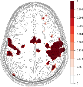
(a)

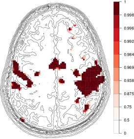
(b)

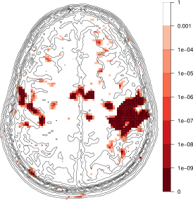
(c)

Figure 1: The posterior probabilities of activation in the fMRI experiment using (a) Swendsen-Wang and (b) single-site updating. (c) Voxel-wise p-values after cluster-wise thresholding for p-values $<0.001$. Displays are in radiological view in the log scale.

In the figure, we only display posterior probabilities that are greater than 0.5. It is clear that the posterior probabilities of activation using either Swendsen-Wang or single-site updating are essentially indistinguishable. For comparison, we have provided the results obtained upon using the commonly-used cluster-wise thresholding of the $p$-values of the test statistic. Here, activation regions are detected by drawing clusters of connected components, each containing a pre-specified number of voxels with $p$-values below a specified threshold [65, 66]. To obtain our activation map, we choose a 2-D second-order neighborhood, a threshold of 0.001 for the $p$-values, following the recommendations of [67], and a minimum cluster size of 4 pixels, as optimally recommended by [68] using the AFNI software [69, 70, 71]. Although a detailed analysis of the results is beyond the scope of this paper, we note from the Bayesian model that there is very high posterior probability of activation in the left primary motor (M1) and pre-motor (pre-M1) cortices and the supplementary motor areas. There are also some areas on the right with high posterior probability of activation, perhaps as a consequence of the left-hand finger-tapping experiment that was also a part of the larger experiment. While the activation maps using cluster-wise thresholding are generally similar to those obtained using Bayesian inference, there are many stray pixels determined to be activated. Moreover, unlike cluster-wise thresholding, Bayesian methods provide us with the posterior probability of activation and this can be used in informing further decisions.

IV-B Establishing first order anisotropy in pistachio tree yields

An unresolved central question in ecology is the degree to which observed cyclic dynamics owe their spatial correlations to endogenous or exogenous factors [72, 73]. Recent work [72] demonstrated (1) as a suitable model for describing long-range synchronization of oscillations in spatial populations. In particular, the binarized yearly increases/decreases in commercial pistachio (Pistacia vera) tree yields, over a $66{\times}106$ grid from 2003 to 2007, shows spatial patterns that can be fitted by an anisotropic Ising model [73]. However, the analysis carried out in [73] could only conclusively establish long-term correlations using the anisotropic model with the binarized dataset for the annual increases/decreases from 2003 to 2004. The authors used a goodness-of-fit measure for pairwise correlation in the horizontal, vertical and diagonal directions [73], with reference distributions calculated by simulation. Our development in Section II-B enables us to easily perform a more formal and principled likelihood ratio test (LRT), as we now demonstrate.

The data are the annual yields (rounded to the nearest pound) from 6,710 female trees at 6,996 locations on a $66{\times}106$ grid [73], for the five-year period of 2003–2007. Let $\boldsymbol{Y}_{(t)}$ be the yield of the trees over the grid in year $t$, for $t\!\in\!\{2003,2004,2005,2006,2007\}$. If a tree is male, or its yield is missing, the value at that grid-point is assumed to be zero. Then, following [73], the first difference field [74] is $\boldsymbol{D}_{(t)}=\boldsymbol{Y}_{(t+1)}{-}\boldsymbol{Y}_{(t)}{-}(\bar{Y}_{(t+1)}{-}\bar{Y}_{(t)})$, where $\bar{Y}_{(t)}$ is the average of the yields in $\boldsymbol{Y}_{(t)}$. The binarized field is then $\boldsymbol{X}_{(t)}$ with $(i,j)$th element given by $\mathbb{I}(\boldsymbol{D}_{ij,(t)}>0)$.

     

(a)

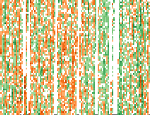
(a) 2003-04

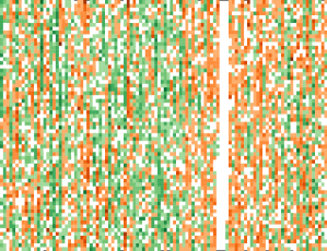
(b) 2004-05

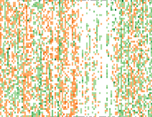
(c) 2005-06

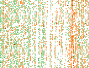
(d) 2006-07

Figure 2: The differences in pistachio yield (in pounds) for female trees in the study area for the year (a) 2003–04, (b) 2004–05, (c) 2005–06 and (d) 2006–07. Red colors indicate negative differences, while green colors indicate positive differences, with darker intensities in both cases corresponding to higher absolute differences. The values are zero for locations with male trees. The binarized version of these yields, that is, binarized in terms of whether these differenced yields are positive (shaded green in each figure) or not, in each field is modeled by an Ising model.

Figure 2 displays the successive differenced yields, which were binarized for our analysis. Under the assumption of an Ising distribution [73], we use a LRT to serially test for independence, neighborhood order, and anisotropy. The general form of the LRT statistic (LRTS) is the same for all these tests, and is

$$\Lambda=\frac{L(\widehat{\alpha}^{0},\widehat{\boldsymbol{\beta}}^{0};\boldsymbol{x})}{L(\widehat{\alpha}^{u},\widehat{\boldsymbol{\beta}}^{u};\boldsymbol{x})},$$ (15)

where $L(\alpha,\boldsymbol{\beta};\boldsymbol{x})$ is the likelihood function, and equals the $\mathbb{P}(\boldsymbol{x};\alpha,\boldsymbol{\beta})$ of (2) when the concerned hypothesis specifies an isotropic Ising model, or is equal to the $\mathbb{P}(\boldsymbol{x};\alpha,\beta_{p},\beta_{v})$ of  (11) when an anisotropic Ising model is specified by the hypothesis. Also $(\widehat{\alpha}^{0},\widehat{\boldsymbol{\beta}}^{0})$ are the maximum likelhihood estimates (MLEs) under the null hypothesis while $(\widehat{\alpha}^{u},\widehat{\boldsymbol{\beta}}^{u})$ are the MLEs under the more general model (comprising the higher loglikelihood under the null and the alternative hypothesis specifications). We note that except for the case of $\boldsymbol{\beta}{=}0$, or independence between the $x_{i}$s, the methods of Section II are needed to obtain the MLE or the maximized likelihood, as well as to compute the $p$-value of each LRTS, which was obtained by simulating 1,000 realizations of the field under the null hypothesis. Indeed, even leaving aside the issue of computational costs, this is a scenario where it is not quite obvious how one may use stochastic methods (such as MCMC) to obtain, for instance, the partition function as a function of $\alpha$ or $\boldsymbol{\beta}$, without recourse to estimating these quantities on a grid, and the interpolating other values. We now detail our investigations.

Our first test is that of independence in the binarized differenced yields at the sites. We consider the isotropic Ising probability model (2) for each binarized differenced field $\boldsymbol{x}$ and test $H_{0}{:}\beta{=}0$ against $H_{a}{:}\beta{\neq}0$, where the field is assumed to follow (1). In this case, with $\bar{x}\doteq n^{-1}\sum_{i=1}^{n}x_{i}$, (15) has the numerator $\bar{x}^{n\bar{x}}(1{-}\bar{x})^{n-n\bar{x}},$ while the denominator is optimized numerically. The $p$-value of the LRTS for each binarized differenced yields is negligible ($p{<}10^{-3}$) in all four cases, and so the null hypothesis of independence is rejected in each of these cases in favor of the isotropic Ising model. We now evaluate anisotropy in these binarized differenced fields.

Table V provides the MLEs of the parameters upon fitting a first-order anisotropic model (11) to each of the binarized differenced yields. In the table, $\beta_{p}$ is the interaction parameter in the horizontal direction, while $\beta_{v}$ is the interaction parameter in the vertical direction. The LRT shows significant evidence of anisotropy for each binarized differenced field. Having established anisotropy, and in light of the displays in Figure 2 we also tested for significance of the horizontal interaction parameter ($\beta_{p}$). We see (Table V) that $\beta_{p}$ is not significant in any of the binarized differenced fields. Finally, we note that [73] found a positive $\alpha$ only in one of the four fields, while our more formal MLEs show positive $\alpha$ estimates in both the middle differenced yields. All $\alpha$s, barring the one obtained from the third differenced field, are significant at the 5% level of significance.

TABLE V: Parameter estimates for the binarized yearly differenced images of pistachio yields ($\boldsymbol{x}$), along with the results of testing for significance. Column 5 displays the $p$-values when testing for the significance of $\alpha$, Column 6 for when testing first order isotropy against first order anisotropy, while Column 7 provides the $p$-values for when testing for a horizontal interaction parameter in the first order anisotropic model.

	Parameters			$p$-value of hypothesis tests
$\boldsymbol{x}$	$\alpha$	$\beta_{v}$	$\beta_{p}$	$H_{0}{:}\alpha{=}0$	$H_{0}{:}\beta_{p}{=}\beta_{v}$	$H_{0}{:}\beta_{p}{=}0$
I	-0.100	0.908	0.319	0.025	$<10^{-3}$	0.395
II	0.035	0.967	0.315	0.028	$<10^{-3}$	0.823
III	0.036	0.948	0.353	0.091	0.002	0.498
IV	-0.069	0.823	0.374	0.026	$<10^{-3}$	0.951

The results of our likelihood-based approach extend the findings of [73], by establishing anisotropy in all the binarized differenced yields. Specifically, previous work [73] was able to conclusively establish anisotropy only for the 2003-04 differenced yields: our approach shows that a first order anisotropic Ising model provides a significantly better fit in all four cases. Further, we show that there is no significant interaction effect in the horizontal direction in either of these binarized differenced yields.

V Discussion

In this paper, we provided explicit approximations for difficult-to-calculate quantities derived from the homogeneous Ising model. In particular, we developed approximations to the partition function, and the moments that are otherwise intractable even for moderate-sized graphs. An R [75] package implementing our approximation formulae is under development and will be released to accompany this paper. We showed that our approximation works well for very realistic lattice sizes and neighborihood structures in the lattices. We stress that our approximations apply to general regular graphs, not necessarily lattices, and with general neighborhood structure. Indeed, its derivation does not use any special graph structure, and only supposes that the graph is regular, that is, that the degree $k$ of each vertex is the same for the entire graph. Recall from the introduction that many researchers have had to simplify their models because of the difficulty in obtaining quantities such as the partition function of more realistic models. Further, unlike the restrictive special cases (such as those considered by [26, 27, 28]) where calculation of the exact partition function is possible, our approach does not grow with the size of the graph and can apply to all dimensions as long as the graph structure is regular. Therefore we expect that our approximation will facilitate the Ising modeling of complex systems by allowing fast and reliable inference. An example of such a situation is a fully Bayesian approach to activation detection in fMRI, which we have demonstrated in Section IV-A can be done quite speedily using our approximations. (This is because our method provides formulae for $Z(\alpha,\beta)$, which would otherwise have to be estimated separately and individually, using stochastic methods for each combination of $\alpha,\beta$ as needed in the MCMC. In essence therefore, our approach when used in fully Bayesian estimation involving a homogeneous Ising model prior, obviates the need for a second layer of MCMC to estimate $Z(\alpha,\beta)$ for each $(\alpha,\beta)$, and therefore can be used in conjunction with the fastest of stochastic algorithms to further speed up computations.) A second application of our methodology, demonstrated in Section IV-B, establishes anisotropy in differenced pistachio tree yields using a formal LRT framework. The LRTS requires ML estimation of the parameters under the null and the more general hypothesis of the null or the alternate hypotheses, and it is our approximate but accurate formulae developed here that make it possible to implement a formal LRT in this application.

A few more comments are in order. The normal approximations of Section II can be computed in ${\cal O}(n)$ operations. However, further approximations obtained by replacing the sums by integrals may be computed much faster depending on the integration method used. We note that the analytical estimates for the mean activation and spin interaction work better for large $k$ because the normal approximation of the distribution of the mean of $r_{h}{=}{\sum_{j}}\eta_{i_{h}j}x_{j}$ is more suited for large $k$.

A possible extension pertains to the case of approximations for the nonhomogeneous Ising model, which is important in a number of applications, such as in item response theory [76]. We feel that it is generally difficult to specify approximation formulae for nonhomogeneous Ising model in the abstract, and that this will depend on the exact specification of the model. However, we also believe that our approximations in this paper will be straightforward to generalize to a locally varying interaction parameter $\beta_{ij}$ if we could somehow decompose the graph into regular components (homogeneous regions with approximately constant degree) where the $\beta_{ij}$s do not change much. In this case, the error in the approximation would probably depend on the size of each component, say $n_{c}$ which are necessarily assumed to be large for our potential approximations to hold.

We close this section with one last comment on the fMRI application. One aspect that has so far not been invoked in fMRI is the fact that it is known that only a very small proportion of about 0.5-2% of voxels are activated in a typical fMRI study [59, 77]. However, this information has never been incorporated satisfactorily in the context of Bayesian activation detection of fMRI. Our approximations in Section II-A2 make it possible to perform Bayesian inference while constraining the prior parameters $(\alpha,\beta)$ so that the a priori proportion of expected activated voxels is satisfied. Thorough development and implementation of such methodology for this application would be of great practical interest for reliably assessing cognition. Thus, we see that while we have addressed an important problem in this paper, there remain issues meriting further attention.

Supplementary Materials

S1 Supplement to Section II

The approximation of $\mbox{I}\!\mbox{E}(M)$ is

$$\begin{split}\tilde{M}_{\phi}(\alpha,\beta_{p},\beta_{v})&=\tfrac{1}{Z_{\tilde{\phi}}(\alpha,\beta_{p},\beta_{v})}\tfrac{\partial}{\partial\alpha}Z_{\tilde{\phi}}(\alpha,\beta_{p},\beta_{v})\\ &=\tfrac{1}{Z_{\tilde{\phi}}(\alpha,\beta_{p},\beta_{v})}\biggl{[}n\exp{(\alpha n)}+n\exp{(\alpha^{\prime\prime})}\\ &\qquad\qquad\qquad\qquad+n(n-1)\exp{\{\alpha(n-2)+\alpha^{\prime\prime}\}}+C_{2,\phi}(\alpha,\beta_{p},\beta_{v})+n\sqrt{\tfrac{n}{2\pi}}\int_{2/n}^{1-2/n}\tfrac{\Delta_{\Phi_{2}}(ny)\exp\{g_{2}(ny)\}}{(1-y)^{n(1-y)+\frac{1}{2}}y^{ny-\frac{1}{2}}}dy\biggr{]},\end{split}$$

where $C_{2,\phi}(\alpha,\beta_{p},\beta_{v})={n\choose 2}\bigl{(}\tfrac{n-2}{2}\exp\{g_{2}(n-2)\}\Delta_{\Phi_{2}}(n-2)+\exp\{g_{2}(2)\}\Delta_{\Phi_{2}}(2)\bigr{)}$. The approximation of $\mbox{I}\!\mbox{E}(S_{p})$ is

$$S_{p,\tilde{\phi}}(\alpha,\beta_{p},\beta_{v})=\tfrac{(nk_{p}/2)}{Z_{\tilde{\phi}}(\alpha,\beta_{p},\beta_{v})}\biggl{[}\exp{(\alpha n)}+(n-2)\exp{\{\alpha(n-2)+\alpha^{\prime\prime}\}}+D_{2,p,\phi}(\alpha,\beta_{p},\beta_{v})+\sqrt{\tfrac{n}{2\pi}}\int_{2/n}^{1-2/n}\tfrac{\tilde{H}_{p}(ny)\exp\{g_{2}(ny)\}}{(1-y)^{n(1-y)+\frac{1}{2}}y^{ny-\frac{3}{2}}}dy\biggr{]},$$

where $nk_{p}D_{2,p,\phi}(\alpha,\beta_{p},\beta_{v})={n\choose 2}\big{[}H_{p}(n-2)\exp\{g_{2}(n-2)\}+H_{p}(2)\exp\{g_{2}(2)\}\big{]}$, with $\tilde{H}_{p}(\ell)=H_{p}(\ell)/(2\ell_{2}\theta_{p})$, and $H_{p}(\ell)=\bigl{\{}\Delta_{\Phi_{2}}(\ell)g_{2,p}(\ell)+\Delta_{\Phi_{2},p}(\ell)\bigr{\}},$ $g_{2,p}(\ell)=\mu_{p,\ell}+\beta_{p}\tau_{p,\ell}^{2}+\beta_{v}\rho_{pv,\ell}\tau_{p,\ell}\tau_{v,\ell},$, and

$$\Delta_{\Phi_{2},p}(\ell)=-\tau_{p,\ell}\biggl{\{}\phi\bigl{(}\tfrac{u^{\bullet}}{\tau_{p,\ell}}\bigr{)}\Delta_{2,\Phi}(u^{\bullet})-\phi\bigl{(}\tfrac{u_{\bullet}}{\tau_{p,\ell}}\bigr{)}\Delta_{2,\Phi}(u_{\bullet})\biggr{\}}-\tfrac{\rho_{pv,\ell}}{\sqrt{1-\rho_{pv,\ell}^{2}}}\int_{u_{\bullet}}^{u^{\bullet}}\phi\bigl{(}\tfrac{u}{\tau_{p,\ell}}\bigr{)}\Delta_{2,\phi}(u)\,du,$$

with $\Delta_{2,\Phi}(u)=\Phi\biggl{(}\tfrac{v^{\bullet}-u\rho_{pv,\ell}\tfrac{\tau_{v,\ell}}{\tau_{p,\ell}}}{\tau_{v,\ell}\sqrt{1-\rho_{pv,\ell}^{2}}}\biggr{)}-\Phi\biggl{(}\tfrac{v_{\bullet}-u\rho_{pv,\ell}\tfrac{\tau_{v,\ell}}{\tau_{p,\ell}}}{\tau_{v,\ell}\sqrt{1-\rho_{pv,\ell}^{2}}}\biggr{)},$ and $\Delta_{2,\phi}(u)=\phi\biggl{(}\tfrac{v^{\bullet}-u\rho_{pv,\ell}\tfrac{\tau_{v,\ell}}{\tau_{p,\ell}}}{\tau_{v,\ell}\sqrt{1-\rho_{pv,\ell}^{2}}}\biggr{)}-\phi\biggl{(}\tfrac{v_{\bullet}-u\rho_{pv,\ell}\tfrac{\tau_{v,\ell}}{\tau_{p,\ell}}}{\tau_{v,\ell}\sqrt{1-\rho_{pv,\ell}^{2}}}\biggr{)}.$

Proceeding in exactly the same manner, we have the approximation of $\mbox{I}\!\mbox{E}(S_{v})$:

$$\begin{split}S_{v,\tilde{\phi}}(\alpha,\beta_{p},\beta_{v})&=\tfrac{1}{2Z_{\tilde{\phi}}(\alpha,\beta_{p},\beta_{v})}\tfrac{\partial}{\partial\beta_{v}}Z_{\tilde{\phi}}(\alpha,\beta_{p},\beta_{v})\\ &=\tfrac{1}{Z_{\tilde{\phi}}(\alpha,\beta_{p},\beta_{v})}\biggl{\{}\tfrac{nk_{v}}{2}\exp(\alpha n)+D_{2,v,\phi}(\alpha,\beta_{p},\beta_{v})+\tfrac{1}{2}\sqrt{\tfrac{n}{2\pi}}\int_{2/n}^{1-1/n}\tfrac{H_{v}(ny)\exp\{g_{2}(ny)\}}{(1-y)^{n(1-y)+\frac{1}{2}}y^{ny+\frac{1}{2}}},dy\biggr{\}},\end{split}$$

where $2D_{2,v,\phi}(\alpha,\beta_{p},\beta_{v})=nH_{v}(n-1)\exp\{g_{2}(n-1)\}+{n\choose 2}H_{v}(2)\exp\{g_{2}(2)\}$, with $H_{v}(\ell)=\bigl{\{}\Delta_{\Phi_{2}}(\ell)g_{2,v}(\ell)+\Delta_{\Phi_{2},v}(\ell)\bigr{\}},$ where $g_{2,v}(\ell)=\mu_{v,\ell}+\beta_{v}\tau_{v,\ell}^{2}+\beta_{p}\rho_{pv,\ell}\tau_{p,\ell}\tau_{v,\ell},$ and

$$\Delta_{\Phi_{2},v}(\ell)=-\tau_{v,\ell}\biggl{\{}\phi\bigl{(}\tfrac{v^{\bullet}}{\tau_{v,\ell}}\bigr{)}\tilde{\Delta}_{2,\Phi}(v^{\bullet})-\phi\bigl{(}\tfrac{v_{\bullet}}{\tau_{v,\ell}}\bigr{)}\tilde{\Delta}_{2,\Phi}(v_{\bullet})\biggr{\}}-\tfrac{\rho_{pv,\ell}}{\sqrt{1-\rho_{pv,\ell}^{2}}}\int_{v_{\bullet}}^{v^{\bullet}}\phi\bigl{(}\tfrac{v}{\tau_{v,\ell}}\bigr{)}\tilde{\Delta}_{2,\phi}(v)\,dv,$$

where $\tilde{\Delta}_{2,\Phi}(v)=\Phi\biggl{(}\tfrac{u^{\bullet}-v\rho_{pv,\ell}\tfrac{\tau_{p,\ell}}{\tau_{v,\ell}}}{\tau_{p,\ell}\sqrt{1-\rho_{pv,\ell}^{2}}}\biggr{)}-\Phi\biggl{(}\tfrac{u_{\bullet}-v\rho_{pv,\ell}\tfrac{\tau_{p,\ell}}{\tau_{v,\ell}}}{\tau_{p,\ell}\sqrt{1-\rho_{pv,\ell}^{2}}}\biggr{)},$ and $\tilde{\Delta}_{2,\phi}(u)=\phi\biggl{(}\tfrac{u^{\bullet}-v\rho_{pv,\ell}\tfrac{\tau_{p,\ell}}{\tau_{v,\ell}}}{\tau_{p,\ell}\sqrt{1-\rho_{pv,\ell}^{2}}}\biggr{)}-\phi\biggl{(}\tfrac{u_{\bullet}-v\rho_{pv,\ell}\tfrac{\tau_{p,\ell}}{\tau_{v,\ell}}}{\tau_{p,\ell}\sqrt{1-\rho_{pv,\ell}^{2}}}\biggr{)}.$

S2 Supplement to Section III

S2-A Normalizing constant for a 2-NN graph

Consider the circular 2-NN Ising model with variables $\{v_{1},\ldots,v_{n}\}\subset\{-1,1\}$ (in this case, $v_{n}$ is a neighbor of $v_{1}$). The corresponding normalizing constant is given by

$$Z_{1}(L,K)=\displaystyle\sum_{\{v\}}\exp\{L\displaystyle\sum_{i}v_{i}+K(v_{n}v_{1}+\displaystyle\sum_{i=1}^{n-1}v_{i}v_{i+1})\}.$$

A well-established result [52, Chapter 13, p. 261] says that for large $n$,

$$\log Z_{1}(L,K){\approx}n\log\left\{\exp(K)\cosh(L){+}\sqrt{\exp(2K)\cosh^{2}(L){-}2\sinh(2K)}\right\}.$$ (S1)

In our setup, the variables $x_{i}\in\{0,1\}$. So we need to transform the variables $v_{i}$ to $x_{i}$. It is easy to see that the corresponding transformation is $x_{i}=(1+v_{i})/2$. so that

$$\begin{split}Z_{1}(L,K)&=\displaystyle\sum_{\{x\}}\exp\left[L\displaystyle\sum_{i}(2x_{i}-1)+K\bigg{\{}(2x_{n}-1)(2x_{1}-1)+\displaystyle\sum_{i=1}^{n-1}(2x_{i}-1)(2x_{i+1}-1)\bigg{\}}\right]\\ &=\exp[n(K-L)]\displaystyle\sum_{\{x\}}\exp\left[2(L-2K)\displaystyle\sum_{i}x_{i}+4K(x_{n}x_{1}+\displaystyle\sum_{i=1}^{n-1}x_{i}x_{i+1})\right].\\ \end{split}$$

From here, we get that $Z_{1}(K,L)=Z(2(L-2K),2K)\exp\{n(K-L)\}$, where the $4K$ is replaced by $2K$ because in our model the sum of over the neighboring vertices is multiplied by two. Therefore, using the fact that the one-nearest-neighbor graph is a regular graph with $k=2$, we get $K=\beta/2$, and $L=\alpha/2$. Consequently, $Z(\alpha,\beta)=\exp\{(\alpha-\beta)(n/2)\}Z_{1}(\alpha/2,\beta/2).$ Using (S1), we obtain for large $n$,

$${\log Z(\alpha,\beta)\approx\frac{n(\alpha-\beta)}{2}+n\log\biggl{[}\exp\left(\tfrac{\beta}{2}\right)\cosh(\alpha/2)+\sqrt{\exp(\beta)\cosh^{2}\left(\tfrac{\alpha}{2}\right)-2\sinh(\beta)}\biggr{]}.}$$

S3 Supplement to Section IV

S3-A Posterior densities for MCMC simulations

1. The parameter $x_{i}$’s: Let $x_{(-i)}=\{x_{1},\ldots,x_{n}\}\setminus\{x_{i}\}$. We propose to update $x_{i}\in\{0,1\}$ via Gibbs’ sampling. The full conditional of the posterior distribution of $x_{i}$, $p(x_{i}\mid x_{(-i)},\Theta_{-x},p)$ is proportional to

   $$\biggl{\{}\bigl{(}C_{B}\bigr{)}^{R}\prod_{r=1}^{R}p_{ri}^{\mu\psi}(1-p_{ri})^{(1-\mu)\psi}\biggr{\}}^{x_{i}}\exp\{\alpha x_{i}-\beta\sum_{j\sim i}(1-\delta_{ij})\},$$

   with $C_{B}=\Gamma(\psi)/\{\Gamma(\mu\psi)\Gamma((1-\mu)\psi)\}$. Let $A_{i}=\alpha+(\mu\psi-1)\sum_{r=1}^{R}\log p_{ri}+\{(1-\mu)\psi-1\}\sum_{r=1}^{R}\log(1-p_{ri})+R\log C_{B}.$ Then $\sum_{r=1}^{R}\log p_{ri}$ is the same as $R\log\check{p}_{i}$ where $\check{p}_{i}$ is the harmonic mean of $\{p_{ri}:r=1,2,\ldots,R\}$. Also, $\sum_{r=1}^{R}\log(1-p_{ri})/R\equiv\log\check{q}_{i}$ where $\check{q}_{i}$ is the harmonic mean of $\{1-p_{ri}:r=1,2,\ldots,R\}$. Then $A_{i}\equiv\alpha+(\mu\psi-1)R\log(\check{p}_{i})+\{(1-\mu)\psi-1\}R\log(\check{q}_{i})+R\log C_{B}$ and

   $$\operatorname{Pr}(X_{i}=1|x_{(-i)},\Theta_{-x},p)\propto\tfrac{\exp(A_{i}-\sum_{j\sim i}\beta)}{\exp(A_{i}-\sum_{j\sim i}\beta)+\exp\{-2(\beta\sum_{j\sim i}x_{j})\}}$$

2. The parameter $\beta$: We have $f(\beta|\Theta_{-\beta},p)\propto{\exp\{-\beta\sum_{i\sim j}(1-\delta_{ij})\}}/{Z(\alpha,\beta)}$, where $Z(\alpha,\beta)$ will be approximated numerically by $\tilde{Z}_{\phi}(\alpha,\beta)$ as defined in Section II-A1. We let $\ddot{\beta}\sim$Gamma$(a,b)$ as our proposed update to $\beta$ with $a/b=\beta$, and $a/b^{2}=\gamma$, for some moderate $\gamma>0$ (e.g., $\gamma=1$). This yields the [78] acceptance ratio that is the minimum of 1 and

   $$\tfrac{\tilde{Z}_{\phi}(\alpha,\beta)}{\tilde{Z}_{\phi}(\alpha,\ddot{\beta})}\tfrac{\Gamma({\beta^{2}}/{\gamma})}{\Gamma({\ddot{\beta}^{2}}/{\gamma})}\exp\biggl{\{}-(\ddot{\beta}-\beta)\sum_{i\sim j}(1-\delta_{ij})+\frac{1}{\gamma}(\ddot{\beta}^{2}-\beta^{2})\log(\beta\ddot{\beta}/\gamma)\biggr{\}}.$$

3. The parameter $\alpha$: The full conditional for $\alpha$ is given by

   $$f(\alpha|\Theta_{-\alpha},p)\propto\exp(\alpha\sum_{i=1}^{n}x_{i})/Z(\alpha,\beta).$$

   Our proposed update to $\alpha$ is $\ddot{\alpha}\sim N(\alpha,\sigma_{\alpha}^{2})$ with a moderate $\sigma^{2}_{\alpha}$, (e.g., $\sigma^{2}_{\alpha}=1$), which, after incorporating the approximation in Section II-A1. is accepted in a [79] step with probability given by $\min\left\{1,{\tilde{Z}_{\phi}(\alpha,\beta)}\exp\{(\ddot{\alpha}-\alpha)\sum_{i=1}^{n}x_{i}\}/{\tilde{Z}_{\phi}(\ddot{\alpha},\beta)}\right\}$.

4. The parameter $\psi$: The full conditional for $\psi$ is given by

   $$f(\psi|\Theta_{-\psi},p)\propto\biggl{[}\tfrac{\Gamma(\psi)}{\Gamma(\mu\psi)\Gamma([1-\mu]\psi)}\biggr{]}^{R\sum_{i}\!x_{i}}\psi^{\zeta-1}\exp[\psi\{\mu\log A+(1-\mu)\log B-\lambda\}],$$

   where $A=\prod_{i=1}^{n}\check{p}_{i}^{Rx_{i}}$, and $B=\prod_{i=1}^{n}\check{q}_{i}^{Rx_{i}}$. Using [50]’s approximation to the factorial function, the right-hand-side of the above equation can be approximated by

   $$\psi^{\frac{1}{2}n_{1}+\zeta-1}\!\exp\biggl{[}-\psi\{\lambda+\operatorname{Ent}(\mu)-\mu\log A-(1-\mu)\log B\}\biggr{]},$$ (S2)

   where $n_{1}=R\sum_{i=1}^{n}x_{i}$, and $\operatorname{Ent}(\mu)=\mu\log\mu+(1-\mu)\log(1-\mu)$ is the negative of the entropy associated with the probabilities $(\mu,1-\mu)$. We update $\psi$ with the proposal $\ddot{\psi}\sim$Gamma$(\tfrac{1}{2}n_{1}+\zeta,\lambda+\operatorname{Ent}(\mu)-\mu\log A-(1-\mu)\log B).$ More generally, we can reduce this updating step to a Gibbs’ sampling step using the above approximated full conditional. The acceptance probability for $\ddot{\psi}$ is the minimum of 1 and

   $$\left(\tfrac{\Gamma(\ddot{\psi})\,\Gamma(\mu\psi)\Gamma((1-\mu)\psi)}{\Gamma(\mu\ddot{\psi})\Gamma((1-\mu)\ddot{\psi})\,\Gamma(\psi)}\right)^{R\sum_{i}\!x_{i}}\biggl{(}\tfrac{\psi}{\ddot{\psi}}\biggr{)}^{\frac{1}{2}n_{1}+\zeta-1}\biggl{(}\tfrac{\ddot{\psi}}{\psi}\biggr{)}^{\zeta-1}\!\!\!\!\exp\bigl{\{}(\ddot{\psi}-\psi)(\mu\log A+(1-\mu)\log B-\lambda)\bigr{\}}\biggr{.}\\ \times\exp\bigl{[}-\{\lambda-\operatorname{Ent}(\mu)-\mu\log A-(1-\mu)\log B\}(\psi-\ddot{\psi})\bigr{]},$$

   which using (S2) yields the approximated acceptance ratio $\min\{1,\exp[(\psi-\ddot{\psi})n_{1}\{\mu\log\mu+(1-\mu)\log(1-\mu)\}]\}$, which is 1 whenever $\ddot{\psi}>\psi$ and so proposals $\ddot{\psi}>\psi$ are always accepted.

5. The parameter $\mu$: Here, we use a random walk update $\ddot{\mu}\sim\operatorname{U}(0,1)$. This yields the Metropolis-Hastings acceptance ratio that is the minimum of 1 and

   $$\biggl{(}\tfrac{\Gamma(\psi)}{\Gamma(\ddot{\mu}\psi)\Gamma((1-\ddot{\mu})\psi)}\tfrac{\Gamma(\mu\psi)\Gamma((1-\mu)\psi)}{\Gamma(\psi)}\biggr{)}^{n_{1}}\,\\ \exp\biggl{\{}\psi\ddot{\mu}\log A+\psi(1-\ddot{\mu})\log B\\ -\psi\mu\log A-\psi(1-\mu)\log B\biggr{\}}.$$

References

- [1] W. Lenz, “Beiträge zum verständnis der magnetischen eigenschaften in festen körpern,” Physikalische Zeitschrift, vol. 21, pp. 613–615, 1920.
- [2] E. Ising, “Beitrag zur theorie des ferromagnetismus,” Z. Physik, vol. 31, pp. 253–258, 1925.
- [3] J. Besag, “On the statistical analysis of dirty pictures,” Journal of the Royal Statistical Society, Series B, vol. 48, no. 3, pp. 259–302, 1986.
- [4] C. Robertson, T. A. Nelson, Y. C. MacNab, and A. B. Lawson, “Review of methods for space–time disease surveillance,” Spatial and Spatio-temporal Epidemiology, vol. 1, pp. 105–116, 2010.
- [5] E. Järpe, “Surveillance of the interaction parameter of the Ising model,” Communications in Statistics - Theory and Methods, vol. 28, no. 12, pp. 3009–3027, 1999.
- [6] D. Lee and R. Mitchell, “Boundary detection in disease mapping studies,” Biostatistics, vol. 13, no. 3, pp. 415–426, 2012.
- [7] H. Ma and B. Carlin, “Bayesian multivariate areal wombling for multiple disease boundary analysis,” Bayesian Analysis, vol. 2, pp. 281–302, 2007.
- [8] H. Ma, B. P. Carlin, and S. Banerjee, “Hierarchical and joint site-edge methods for Medicare hospice service region boundary analysis,” Biometrics, vol. 66, no. 2, pp. 355–364, 2010.
- [9] A. Irback, C. Peterson, and F. Potthast, “Evidence for nonrandom hydrophobicity structures in protein chains,” Proceedings of the National Academy of Sciences USA, vol. 93, pp. 9533–9538, 1996.
- [10] G. Rowe and L. Trainor, “A thermodynamic theory of codon bias in viral genes,” Journal of Theoretical Biology, vol. 101, pp. 171–203, 1983.
- [11] A. Ahsan, J. Rudnick, and R. Bruinsma, “Elasticity theory of the B-DNA to S-DNA transition,” Biophysical Journal, vol. 74, pp. 132–137, 1998.
- [12] Y. Liu and J. Dilger, “Application of the one- and two-dimensional Ising models to studies of cooperativity between ion channels,” Biophysical Journal, vol. 64, pp. 26–35, 1993.
- [13] E. Schneidman, M. Berry, R. Segev, and W. Bialek, “Weak pairwise correlations imply strongly correlated network states in a neural population,” Nature, vol. 440, pp. 1007–1012, 2006.
- [14] S. Yu, D. Huang, W. Singer, and D. Nikolic, “A small world of neuronal synchrony,” Cerebral Cortex, vol. 18, pp. 2891–2901, 2008.
- [15] L. Hamilton, J. Sohl-Dickstein, A. Huth, V. Carels, K. Deisseroth, and S. Bao, “Optogenetic activation of an inhibitory network enhances feedforward functional connectivity in auditory cortex,” Neuron, vol. 80, no. 4, p. 1066–1076, 2013.
- [16] E. Ganmor, R. Segev, and E. Schneidman, “Sparse low-order interaction network underlies a highly correlated and learnable neural population code,” Proceedings of the National Academy of Sciences USA, vol. 108, pp. 9679–9684, 2011.
- [17] E. Baake, M. Baake, and H. Wagner, “Ising quantum chain is equivalent to a model of biological evolution,” Physical Review Letters, vol. 78, no. 3, p. 1782, 1997.
- [18] O. Banerjee, L. E. Ghaoui, and A. d’Aspremont, “Model selection through sparse maximum likelihood estimation for multivariate gaussian or binary data,” Journal of Machine Learning Research, vol. 9, pp. 485–516, 2008.
- [19] S. Wasserman and P. Pattison, “Logit models and logistic regressions for social networks: I. An introduction to Markov graphs and ,” Psychometrika, vol. 61, no. 3, pp. 401–425, 1996.
- [20] K. Klemm, V. M. Eguíluz, R. Toral, and M. San-Miguel, “Nonequilibrium transitions in complex networks: A model of social interaction,” Physical Review E, vol. 67, p. 026120, 2003.
- [21] F. Barahona, “On the computational complexity of ising spin glass models,” J. Phys. A: Math. Gen., vol. 15, pp. 3241–3253, 1982.
- [22] R. Maitra and J. E. Besag, “Bayesian reconstruction in synthetic Magnetic Resonance Imaging,” in Proceedings of the Society of Photo-Optical Instrumentation Engineers (SPIE 1998) Meetings, A. Mohammad-Djafari, Ed., vol. 3459, 1998, pp. 39–47.
- [23] J. Majewski, H. Li, and J. Ott, “The Ising model in physics and statistical genetics,” The American Journal of Human Genetics, vol. 69, pp. 853–862, 2001.
- [24] L. Reichl, A modern course in statistical physics. Austin, TX: University of Texas Press, 1980.
- [25] Q. Mo and F. Liang, “A hidden Ising model for ChIP-chip data analysis,” Bioinformatics, vol. 26, no. 6, pp. 777–783, 2010.
- [26] B. Kaufman, “Crystal statistics. ii. partition function evaluated by spinor analysis,” PHYSICAL REVIEW, vol. 76, no. 8, pp. 1232–1243, 1949.
- [27] N. N. Schraudolph and D. Kamenetsky, “Efficient exact inference in planar ising models,” in Advances in Neural Information Processing Systems 21, D. Koller, D. Schuurmans, Y. Bengio, and L. Bottou, Eds. Curran Associates, Inc., 2009, pp. 1417–1424.
- [28] Y. M. Karandashev and M. Y. Malsagov, “Polynomial algorithm for exact calculation of partition function for binary spin model on planar graphs,” Optical Memory and Neural Networks, vol. 26, no. 2, pp. 87–95, Apr 2017.
- [29] Y. Ogata, “A Monte Carlo method for high dimensional integration,” Numerische Mathematik, vol. 55, pp. 137–157, 1989.
- [30] A. Gelman and X. L. Meng, “Simulating normalizing constants: from importance sampling to bridge sampling to path sampling,” Statistica Sinica, vol. 13, pp. 163–185, 1998.
- [31] S. Richardson and P. J. Green, “On Bayesian analysis of mixtures with an unknown number of components,” Journal of the Royal Statistical Society, Series B, vol. 59, pp. 731–792, 1997.
- [32] F. Wang and D. P. Landau, “Efficient, multiple-range random walk algorithm to calculate the density of states,” Physical Review Letter, vol. 86, pp. 2050–2053, 2001.
- [33] A. M. Ferrenberg and R. H. Swendsen, “Optimized Monte Carlo data analysis,” Physics Review Letters, vol. 63, no. 12, p. 1195, 1989.
- [34] S. Kumar, D. Bouzida, S. R. H., P. A. Kollman, and J. M. Rosenberg, “The weighted histogram analysis method for free-energy calculations on biomelecules. I. The method,” Journal of Computational Chemistry, vol. 3, no. 8, pp. 1011–1021, 1992.
- [35] Y. F. Atchade and J. S. Liu, “The Wang-Landau algorithm in general state spaces: applications and convergence analysis,” Statistica Sinica, vol. 20, pp. 209–233, 2010.
- [36] Y. F. Atchade, N. Lartillot, and C. P. Robert, “Bayesian computation for statistical models with intractable normalizing constants,” Brazilian Journal of Probability and Statistics, vol. 27, no. 4, pp. 416–436, 2013.
- [37] F. Liang, “A generalized Wang-Landau algorithm for Monte-Carlo computation,” Journal of the American Statistical Association, vol. 100, no. 472, pp. 1311–1327, 2005.
- [38] P. Del Moral, A. Doucet, and A. Jasra, “Sequential Monte Carlo samplers,” Journal of the Royal Statistical Society, Series B, vol. 68, pp. 411–436, 2006.
- [39] F. Liang, “A double metropolis–hastings sampler for spatial models with intractable normalizing constants,” Journal of Statistical Computation and Simulation, vol. 80, no. 9, pp. 1007–1022, 2010.
- [40] F. Liang, I. H. Jin, Q. Song, and J. S. Liu, “An adaptive exchange algorithm for sampling from distributions with intractable normalizing constants,” Journal of the American Statistical Association, vol. 111, no. 513, pp. 377–393, 2016.
- [41] Q. Zhang and F. Liang, “Bayesian analysis of exponential random graph models using stochastic gradient markov chain monte carlo,” Bayesian Analysis, vol. 1, no. 1, pp. 1–27, 2023.
- [42] A. M. Lyne, M. Girolami, Y. Atchadé, H. Strathmann, and D. Simpson, “On russian roulette estimates for bayesian inference with doubly-intractable likelihoods,” Statistical Science, vol. 30, no. 4, pp. 443–467, 2015.
- [43] J. Park and M. Haran, “A function emulation approach for doubly intractable distributions,” Journal of Computational and Graphical Statistics, vol. 29, no. 1, pp. 66–77, 2020.
- [44] A. Boland, N. Friel, and F. Maire, “Efficient mcmc for gibbs random fields using precomputation,” Electronic Journal of Statistics, vol. 12, p. 4138–4179, 2018.
- [45] C. J. Geyer, “Likelihood inference for spatial point processes,” Stochastic geometry: likelihood and computation, vol. 80, pp. 79–140, 1999.
- [46] B. Bollobás, Random Graphs, 2nd ed. Cambridge: Cambridge University Press, 2001.
- [47] Z. Govindarajulu, “Normal approximations to the classical discrete distributions,” Sankya: The Indian Journal of Statistics, Series A, vol. 27, no. 2, pp. 143–172, 1965.
- [48] W. Hoeffding, “Probability inequalities for sums of bounded random variables,” Journal of the American Statistical Association, vol. 58, no. 301, pp. 13–30, 1963.
- [49] M. Abramowitz and I. A. Stegun, Handbook of Mathematical Functions with Formulas, Graphs, and Mathematical Tables, Ninth Dover printing, tenth GPO printing ed. New York: Dover, 1964.
- [50] J. Stirling, Methodus Differentialis, London, 1730.
- [51] R. H. Swendsen and J.-S. Wang, “Nonuniversal critical dynamics in Monte Carlo simulations,” Physical Review Letter, vol. 58, pp. 86–88, 1987.
- [52] S. Salinas, Introduction to Statistical Physics. Springer, 2001.
- [53] M. D. McKay, R. J. Beckman, and W. J. Conover, “A comparison of three methods for selecting values of input variables in the analysis of output from a computer code,” Technometrics, vol. 42, no. 1, pp. 55–61, 2000.
- [54] W. Press, S. Teukolsky, W. Vetterling, and B. Flannery, Numerical Recipes in C: The art of scientific computing, 2nd ed. Cambridge University Press, 1996.
- [55] J. A. Nelder and R. Mead, “A simplex method for function minimization,” The Computer Journal, vol. 7, no. 4, pp. 308–313, 1965.
- [56] J. Besag, “Statistical analysis of non-lattice data,” The Statistician, vol. 24, no. 3, pp. 179–195, 1975.
- [57] B. C. Arnold and D. Strauss, “Pseudolikelihood estimation: some examples,” Sankhya, Series B, vol. 53, pp. 233–243, 1991.
- [58] G. Gong and F. J. Samaniego, “Pseudo maximum likelihood estimation: theory and applications,” The Annals of Statistics, vol. 9, no. 4, pp. 861–869, 1981.
- [59] N. A. Lazar, The Statistical Analysis of Functional MRI Data. Springer, 2008.
- [60] M. A. Lindquist, “The statistical analysis of fmri data,” Statistical Science, vol. 23, no. 4, pp. 439–464, 2008.
- [61] R. Maitra, S. R. Roys, and R. P. Gullapalli, “Test-retest reliability estimation of functional mri data,” Magnetic Resonance in Medicine, vol. 48, pp. 62–70, 2002.
- [62] R. Maitra, “Assessing certainty of activation or inactivation in test-retest fMRI studies,” Neuroimage, vol. 47, pp. 88–97, 2009.
- [63] ——, “A re-defined and generalized percent-overlap-of-activation measure for studies of fmri reproducibility and its use in identifying outlier activation maps,” Neuroimage, vol. 50, pp. 124–135, 2010.
- [64] S. Z. Li, Markov Random Field Modeling in Image Analysis, 3rd ed. London: Springer-Verlag, 2009.
- [65] K. J. Friston, P. Jezzard, and R. Turner, “Analysis of functional mri time-series,” Human Brain Mapping, vol. 1, pp. 153–171, 1994.
- [66] S. Hayasaka and T. E. Nichols, “Validating cluster size inference: random field and permutation methods,” Neuroimage, vol. 20, p. 2343–2356, 2003.
- [67] C.-W. Woo, A. Krishnan, and T. D. Wager, “Cluster-extent based thresholding in fMRI analyses: Pitfalls and recommendations,” Neuroimage, vol. 91, p. 412–419, 2014.
- [68] S. Forman, J. Cohen, M. Fitzgerald, W. Eddy, M. Mintun, and D. Noll, “Improved assessment of significant activation in functional magnetic resonance imaging (fMRI): use of a cluster-size threshold,” Magnetic Resonance in Medicine, vol. 33, p. 636–647, 1995.
- [69] R. W. Cox, “AFNI: software for analysis and visualization of functional magnetic resonance neuroimages,” Computers and biomedical research, an international journal, vol. 29, no. 3, pp. 162–173, 1996.
- [70] R. W. Cox and J. S. Hyde, “Software tools for analysis and visualization of fMRI data,” NMR in Biomedicine, vol. 10, no. 4-5, pp. 171–178, 1997.
- [71] R. W. Cox, “AFNI: What a long strange trip it has been,” NeuroImage, vol. 62, pp. 743–747, 2012.
- [72] A. E. Noble, J. Machta, and A. Hastings, “Emergent long-range synchronization of oscillating ecological populations without external forcing described by Ising universality,” Nature Communications, vol. 6, 2015.
- [73] A. E. Noble, T. S. Rosenstock, P. H. Brown, J. Machta, and A. Hastings, “Spatial patterns of tree yield explained by endogenous forces through a correspondence between the Ising model and ecology,” Proceedings of the National Academy of Sciences, vol. 115, no. 8, pp. 1825–1830, 2018. [Online]. Available: https://www.pnas.org/doi/abs/10.1073/pnas.1618887115
- [74] G. E. P. Box and G. M. Jenkins, Time Series Analysis: Forecasting and Control. San Francisco: Holden–Day, 1970.
- [75] R Core Team, R: A Language and Environment for Statistical Computing, R Foundation for Statistical Computing, Vienna, Austria, 2023. [Online]. Available: https://www.R-project.org/
- [76] C. D. Van Borkulo, D. Borsboom, S. Epskamp, T. F. Blanken, L. Boschloo, R. A. Schoevers, and L. J. Waldorp, “A new method for constructing networks from binary data,” Scientific Reports, vol. 4, no. 1, p. 5918, 2014.
- [77] W.-C. Chen and R. Maitra, “A practical model-based segmentation approach for improved activation detection in single-subject functional magnetic resonance imaging studies,” Human Brain Mapping, vol. 44, no. 16, pp. 5309–5335, 2023.
- [78] W. K. Hastings, “Monte carlo sampling methods using markov chains and their applications,” Biometrika, vol. 57, no. 1, pp. 97–109, 1970.
- [79] N. Metropolis, A. W. Rosenbluth, M. Rosenbluth, A. H. Teller, and E. Teller, “Equations of state calculations by fast computing machines,” Journal of Chemical Physics, vol. 21, pp. 1087–1092, 1953.