Double $K^{0}_{S}$ Photoproduction off the Proton at CLAS

Abstract

The $f_{0}(1500)$ meson resonance is one of several contenders to have significant mixing with the lightest glueball. This resonance is well established from several previous experiments. Here we present the first photoproduction data for the $f_{0}(1500)$ via decay into the $K_{S}^{0}K_{S}^{0}$ channel using the CLAS detector. The reaction $\gamma p\to f_{J}p\rightarrow K_{S}^{0}K_{S}^{0}p$, where $J=0,2$, was measured with photon energies from 2.7 to 5.1 GeV. A clear peak is seen at 1500 MeV in the background subtracted invariant mass spectra of the two kaons. This is enhanced if the measured 4-momentum transfer to the proton target is restricted to be less than 1.0 GeV². By comparing data with simulations, it can be concluded that the peak at 1500 MeV is produced primarily at low $t$, which is consistent with a $t$-channel production mechanism.

I Introduction

The search for glueballs has been ongoing for several decades key-1 . The lightest glueball has been predicted by quenched lattice QCD to have a mass in the range of $1.5-1.8$ GeV and $J^{PC}=0^{++}$ key-2 . The mixing of glueball states with neighbouring meson states complicates their identification and hence possible glueball candidates have been extensively scrutinized.

Of the scalar mesons, the isoscalars are the mesons of interest in the search for glueballs. Five isoscalar scalars have been identified by experiment and listed by the Particle Data Group (PDG): $f_{0}(500)$, $f_{0}(980)$, $f_{0}(1370),$ $f_{0}(1500)$ and $f_{0}(1710)$ key-3 . However, of these, only two can belong to the meson scalar nonet (see the tentative assignments given in Ref. key-3 ). As discussed below, two of these states (the $f_{0}(500)$ and $f_{0}(980)$), are thought to be either meson-meson molecules or $qq\bar{q}\bar{q}$ states, but this still leaves three possible scalar mesons to fit into two quark-model slots. The excess of scalar states suggests the presence of a glueball state, with the same quantum number ($J^{PC}=0^{++}$), which mixes with the scalar meson states key-1 . By analyzing the decay channels and production mechanisms of these three scalar meson candidates, the glueball mixing can be compared with theoretical predictions.

In reality, there is no consensus on the status of several of these scalars key-3 . For some scalar mesons, such as the $f_{0}(500)$, the distinction between resonance and background is difficult because of the large decay widths. Also, the opening of multiple decay channels within short mass intervals makes the background shapes difficult to model key-3 . Yet the high interest for a possible glueball state (and how it mixes with the scalar mesons) motivates further measurements of the production mechanisms and decays of the scalars.

After many years and many experiments focused on the scalar mesons, there is still confusion on how to classify these states key-3 . The $f_{0}(980)$ and the $a_{0}(980)$, along with the $f_{0}(500)$ and $K_{0}^{*}(800)$, likely form a low-mass nonet of primarily four-quark states key-4 ; key-5 . Models based on unitary quarks with coupled $q\bar{q}$ and meson-meson channels interpret the scalars as two nonets, the {$f_{0}(980)$, $a_{0}(980)$, $f_{0}(500)$ and $K_{0}^{*}(800)$}, and the {$f_{0}(?)$, $a_{0}(1450)$ and $K_{0}^{*}(1430)$}, where $f_{0}(?)$ stands for two of the $f_{0}(1370)$, $f_{0}(1500)$ or $f_{0}(1710)$. These are two expressions of the same bare states key-3 ; key-4 , where the former nonet is consistent with a dominant $qq\bar{q}\bar{q}$ component. In the latter nonet, the $f_{0}(1500)$ and the $f_{0}(1710)$ are candidates for having the highest glueball content key-1 .

Recently, there has been a resurgence of interest in the $f_{0}(1710)$ as the best glueball candidate based on Holographic QCD calculations key-6 . In that paper, they calculate the glueball decay rates and find a suppressed decay of the glueball into final states with two pions (and also a very small coupling to four-pion decay). The decay ratio of $\Gamma(\pi\pi)/\Gamma(KK)$ for the $f_{0}(1710)$ is found key-3 to be much smaller than the $SU(3)_{F}$ value of 3/4, giving better agreement with their predictions. However, as pointed out above, the experimental measurements of these scalar meson decays is sometimes conflicting key-3 , and hence more measurements are needed.

Figure 1: Schematic diagrams of reaction mechanisms for (a) $s$-channel and (b) $t$-channel photoproduction of a scalar meson.

Photoproduction has been suggested as a means to look for glueballs key-7 . Production can occur primarily via two channels, as shown in Fig. 1. In the $s$-channel, the photon and proton interact to form an intermediate particle that then decays into a meson and a proton. This channel can couple directly to a scalar meson with high glueball content. In the $t$-channel on the other hand, the photon must couple to the exchange particle. In this case, the outgoing particle (and hence the exchange particle) has neutral charge, and the photon coupling is suppressed. For a pure $SU(3)_{F}$ glueball key-2 , made entirely of gluons (with no quark-antiquark pairs), there is no charge and hence no coupling to the photon. For a meson with a large glueball admixture, the photon coupling in $t$-channel is expected to be partly suppressed brodsky , since its wavefunction contains a glueball component.

The $t$-channel strength can be separated, to a large extent, from $s$-channel by measuring the 4-vectors of the detected particles and calculating the momentum transfer, $|t|$, to the proton. Low values of momentum transfer typically correspond to $t$-channel diagrams, whereas $s$-channel diagrams span a wider range of momentum transfer.

Here, we examine the photoproduction of scalar and tensor mesons at energies from $\sqrt{s}=$2.4 to 3.3 GeV, spanning an energy region above threshold to produce scalar $f_{0}$ mesons off a proton target. The following sections provide the experimental details and the analysis procedures used to study the $t$-dependence of the yeild for one of these states with a mass near 1500 MeV. While the statistics are low, making it difficult to draw firm conclusions on the spin $J$ of the peak at 1500 MeV, the data validates the technique, and future measurements with higher statistics at Jefferson Lab will provide more conclusive results.

II Experimental Setup

The experiment was carried out in Hall B at the Thomas Jefferson National Accelerator Facility using the CEBAF Large Acceptance Spectrometer (CLAS) key-8 . The primary electron beam from the CEBAF accelerator struck a gold foil of $10^{-4}$ radiation lengths, producing a tagged real photon beam key-9 . The photon energy was determined from the trajectory of the detected electron in the tagger focal plane. The initial electron energy for this experiment, called g12, was 5.71 GeV and the tagged photon energy range was between 20% to 95% of the initial electron energy. The photon energy resolution depends on energy and was $<7.6$ MeV. The g12 data were taken from April to June, 2008, with a beam of polarized electrons (the photon beam polarization was not used in the present analysis).

The photons struck a liquid hydrogen target of length 40 cm and diameter 4 cm. The target was placed 90 cm upstream of the center of CLAS in order to improve the acceptance for particles produced at small angles. Final state hadrons from the photon-nucleon interactions went into a toroidal magnetic field produced by the six-sector coils of the CLAS detector key-8 . The coils were run with a current of 1930 A, which is half of the maximum design current. Positively charged particles were bent away from the beamline, thus having a larger detector acceptance than negatively charged particles of the same momentum.

Particles were tracked using a set of three drift chambers in each sector key-10 , giving a momentum resolution of $\sim$0.5% for charged particles of momentum $p=1$ GeV/c. The time of flight of the particles was measured between a start counter that surrounded the target key-11 and an array of scintillator bars that covered the exterior of the CLAS detector key-8 . A photon in the tagger along with at least two charged particles in a timing coincidence produced a trigger for the data acquisition system. Details of the trigger can be found in Ref. key-12 .

III Analysis Procedures

The reactions

$$\gamma p\rightarrow f_{0}p\ \ {\rm and}\ \ \gamma p\rightarrow f_{2}p$$ (1)

were studied in the decay branch

$$f_{J}\rightarrow K_{S}^{0}+K_{S}^{0}\rightarrow\pi^{+}\pi^{-}\pi^{+}\pi^{-}\ .$$ (2)

In the above reactions, the photon beam and the proton target interact to produce a scalar (tensor) meson and the proton. The scalar (tensor) meson then decays into a pair of short lived neutral kaons ($K_{S}^{0}$), each of which decay into a pair of charged pions. The final state particles are $\pi^{+}\pi^{-}\pi^{+}\pi^{-}p$, of which the four charged pions are detected, while the proton is identified via the missing mass technique. Requiring the final state to be $K_{S}K_{S}$ (four detected pions) ensures that the $CP$ of the resonant meson is $++$. This limits the final state meson to have even $J$, and we expect $J=0,2$ to dominate near threshold.

The trigger configurations, calibrations of the detector sub-systems, and determination of the photon flux have been detailed in Ref. key-12 .

III.1 The Basic Cuts

The basic analysis cuts (event selection criteria) and momentum corrections that are applied to the data are listed in Table 1. These will be discussed in Sections III.1.1 through III.1.6. Kinematic cuts are described in Section III.1.7.

Cut Level	Type of Cut	Size of Cut
1	Timing Cut for identification of pions	$\pm 1$ ns
2	Fiducial Cut	Fit to CLAS acceptance
3	Missing mass (proton)	$\pm$0.0497 GeV (3$\sigma$)
4	Photon beam energy	2.7-3.0 and 3.1-5.1 GeV
5	$K_{S}^{0}$ peak and sideband subtraction	0.01614 GeV (3$\sigma$)

Table 1: The event selection criteria (cuts) used in this analysis.

III.1.1 Timing Cut

During the time that the DAQ recorded one event, several photons could be measured by the tagger. Of these photons, it was necessary to find that photon which interacted with the target to produce the particles in CLAS. The tracks measured in the drift chamber (DC) were extrapolated to the start counter and also to the Time-of-Flight (TOF) scintillator bars. Using time and distance measurements, the start time for every track was calculated. The beam RF time corresponding to the start times for all tracks, corrected for the vertex position in the target, was taken as the event vertex time.

To identify and select the detected particles as pions, the TOF Difference method was employed. In this method, the difference between the calculated and measured time of flight was constrained to be within 1 ns. The calculated TOF was determined in the following manner: the mass of the particles was assumed to be the mass of the charged pion, 139.57 MeV. Then, using the measured momentum of the particle, we can calculated the time required by the $\pi^{+}$or $\pi^{-}$ to traverse the path, $L_{sc}$, from the target to the TOF:

$$\beta_{calc}=\frac{p_{measured}}{\sqrt{p_{measured}^{2}+m_{\pi}^{2}}}$$ (3)

and

$$TOF_{calc}=\frac{L_{sc}}{c\beta_{calc}}\ ,$$ (4)

where $c$ is the speed of light.

The measured TOF is the difference in time of the scintillator hit, $t_{sc}$, and the event vertex time,

$$TOF_{measured}=t_{sc}-t_{vertex}\ .$$ (5)

The difference between the measured and calculated TOF,

$$\Delta TOF=TOF_{measured}-TOF_{calc}\ ,$$ (6)

was calculated and a $\pm 1.0$ ns cut on $\Delta TOF$ was applied. If this cut led to the selection of at least two positively charged pions and at least two negatively charged pions, then the event was passed on for further analysis.

The photon whose vertex time matched most closely to the average start counter time of the pions was chosen. Depending on the electron beam current, there could be more than one “good” photon. Using the four-momenta of the four pions, the target proton and the photon, the missing mass off of the four pions was calculated. If a single photon was within the missing mass cut (see Cut 3 of Table 1) then this photon was chosen. After this selection, the events with one good photon accounted for 96% of the total events with 2$\pi^{+}$ and 2$\pi^{-}$.

III.1.2 Fiducial Cut

The CLAS torus magnet consisted of six superconducting coils arranged to form a toroid around the beamline. In the rare case where one of the decay particles hit support material and scattered into the detector, an improper track would be observed. Also particle tracks reconstructed very near the coils could be inaccurate due to slight distortion of the magnetic field. Therefore, it is useful to apply fiducial cuts to reject those particles that track into the regions immediately surrounding the coils. Such cuts were employed here, which trimmed a few percent off the edges of the active region of the CLAS detector. Details on the fiducial cuts are available elsewhere key-12 .

III.1.3 Energy Loss Corrections

To account for the energy loss of the decay particles while traversing through the target, start counter and their associated assembly materials, the CLAS $eloss$ package key-14 was employed. It corrected for the loss of energy using the Bethe-Bloch equation, which relates the energy loss of a particle through a material with the characteristics of the material and the distance traveled by the particle in that material. This software package had all of the geometry of the target and the surrounding material, so that each track was corrected for energy loss according to its trajectory.

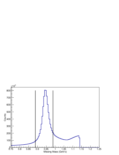
Figure 2: Missing mass for the reaction $\gamma p\to 2\pi^{+}2\pi^{-}X$ was calculated from the incident photon energy, the target proton mass and the momentum of the detected charged pions. A clear peak is seen at the mass of the proton. The vertical lines enclose the selected events.

III.1.4 Missing Mass Cut

The missing particle in the reaction is calculated using the four-momenta of detected pions, beam and target:

$$P_{miss}=(P_{beam}+P_{target})-(P_{\pi^{+}}+P_{\pi^{-}}+P_{\pi^{+}}+P_{\pi^{-}})\ .$$ (7)

The missing particle was then defined to be the proton by selecting those events that had a missing mass within $\sim$50 MeV of the mass of the proton (Cut 3 in Table 1), as shown in Fig. 2. Only the particle identification and fiducial cuts are applied in Fig. 2. The small background under the proton peak was significantly reduced after further analysis cuts were employed.

III.1.5 Beam Energy Cut

The threshold photon energy for the production of the $f_{0}(1500)$, which is the particle of main interest, can be calculated by means of the following equation:

$$E_{\gamma^{min}}=\frac{m_{f_{0}(1500)}^{2}+2m_{f_{0}(1500)}m_{p}}{2m_{p}}\ .$$ (8)

From this, the minimum energy to produce a $f_{0}(1500)$ in this reaction is $E_{\gamma^{min}}=2.7$ GeV. Since we are interested in studying the $f_{0}(1500)$, photon energies below 2.7 GeV were removed in further analysis. For the g12 experiment, there is a discontinuity in $E_{\gamma}$ at $\sim 3$ GeV due to a bad timing counter in the photon tagger. This region is excluded from the analysis by eliminating the events between 3.0 and 3.1 GeV for both data and simulations. This event selection (Cut 4 in Table 1) has been applied to all of the following figures.

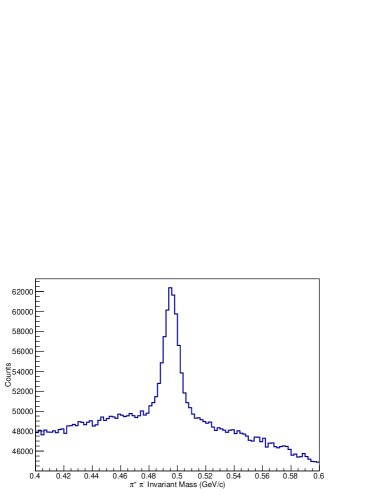
Figure 3: Invariant mass spectrum for one combination of $\pi^{+}\pi^{-}$. A clear $K_{S}^{0}$ peak is seen over a two-pion background. Other combinations show a similar mass distribution.

III.1.6 Sideband Subtraction

The four pions, $\pi_{1}^{+},\pi_{1}^{-},\pi_{2}^{+}$ and $\pi_{2}^{-}$ can form $2K_{S}^{0}$ in two ways. We use the following naming convention:

$$K1=\pi_{1}^{+}\pi_{1}^{-},\ \ \ K2=\pi_{2}^{+}\pi_{2}^{-}$$ (9)

and

$$K3=\pi_{1}^{+}\pi_{2}^{-},\ \ \ K4=\pi_{2}^{+}\pi_{1}^{-}\ .$$ (10)

The numbering of the pions was based on the order in which they were recorded by the event builder software. In order to avoid any bias, the ordering was randomized in our analysis. In a given event, the 4 pions can form either: (a) $K1$ and $K2$ or (b) $K3$ and $K4$. Figure 3 shows the invariant mass spectrum for the first pair of $\pi^{+}\pi^{-}$, which shows a clear $K_{S}^{0}$ peak above a nearly flat background. Because we randomized the ordering of the pions, other combinations show similar invariant mass distributions.

If the invariant masses of the pairs of pions are plotted against one another, a strong correlation is observed (if one pair forms a $K_{S}^{0}$, then the other pair is very likely to form a second $K_{S}^{0}$, indicating a common decay source for a majority of the events). In order to reduce background under the $K_{S}^{0}$ peak, a standard method of background subtraction is used. A $3\sigma$ region (see Cut 5 of Table 1) is applied around the $K_{S}^{0}$ mass to identify events lying in the signal region. Since the background is relatively flat, the bands on either side of the signal can be considered to be the average background below the $K_{S}$ peak. These regions are of the same width as the signal region and are referred to as sidebands.

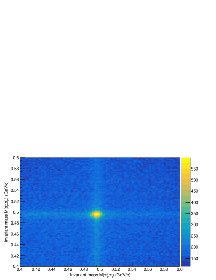
Figure 4: Correlation between the invariant mass of one $\pi^{+}\pi^{-}$ pair and the other $\pi^{+}\pi^{-}$ pair. The spot at the center shows the situation where both pion pairs come from decays of two $K_{S}^{0}$.

A 2-dimensional plot of the invariant masses of one pair of pions versus the other is shown in Fig. 4, where a clear $K_{S}^{0}$-$K_{S}^{0}$ correlation is seen. The signal region is a square centered on the $K_{S}^{0}$ mass (on each axis). Also, there are several sideband regions to consider. Each sideband region is a square, sharing one edge (or one corner) with the signal region and with its center offset by $6\sigma$ from the center of the signal region. Note that there are faint horizontal and vertical lines that go through the signal and sideband regions. These are likely due to events where one $K_{S}^{0}$ and a strange baryon resonance ($\Sigma^{*}$) were produced, followed by a decay such as $\Sigma^{*+}\to\Lambda\pi^{+}\to p\pi^{-}\pi^{+}$. These events were subtracted, in the correct proportion, from the background under the signal region by using the sidebands.

Figure 5 shows the $4\pi$ invariant mass spectrum before and after background subtraction. This mass spectrum is virtually identical to that formed from the $2K_{S}^{0}$ invariant mass. We choose to plot it this way because the average of the sideband regions are plotted together with the signal region. Two clear peaks, one at $\sim 1.28$ GeV and another at 1.5 GeV are seen in the sideband-subtracted mass spectrum. There is the hint of a possible peak (or fluctuation) near 1.75 GeV, but it is not statistically significant and will be investigated in future higher-statistics data sets acquired with CLAS12.

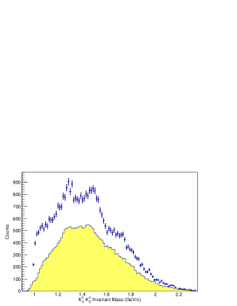
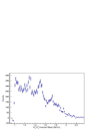
Figure 5: The left histogram with the error bars shows the signal + background, whereas the shaded (yellow online) histogram is the average sideband background. The right histogram is the sideband subtracted histogram. The peak near 1.50 GeV is the region of interest.

III.1.7 Momentum Transfer Cut

In the invariant mass spectrum in Fig. 5 the resonance of interest is the one at 1.50 GeV. In order to further investigate it, cuts on the momentum transfer, $t$, were applied,

$$t=(P_{beam}-P_{K_{S}^{0}}^{1}-P_{K_{S}^{0}}^{2})^{2}\ ,$$ (11)

where $P_{K_{S}^{0}}^{1,2}$ are the 4-momenta of the two $K_{S}^{0}$, each made from the 4-momenta of two charged pions.

In Fig. 6 (left), where the cut $|t|<1$ GeV² has been applied, the 1.50 GeV resonance is enhanced in the spectrum, whereas it disappears for $|t|>1$ GeV², as shown in Fig. 6 (right). If an $s$-channel production mechanism was involved, we would have expected to see the peak over a wider range of $t$ (within the available phase space). The $t$-dependence of the peak at 1.50 GeV is consistent with a meson exchange process (a $t$-channel diagram, Fig. 1).

The choice to cut at $|t|=1$ GeV² is somewhat arbitrary, but is a reasonable attempt to separate small and large momentum transfer. For example, if there is $\rho$-exchange in a $t$-channel diagram, this would contribute more significantly at $|t|<1$ GeV², where the momentum transfer is a better match with the mass of the $\rho$ meson. Choosing a slightly different value for the cut on $|t|$ does not change our conclusions.

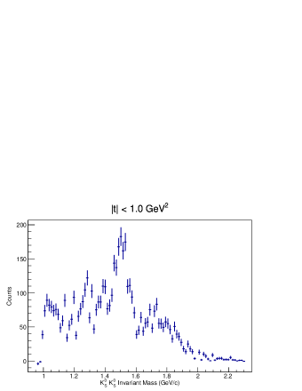
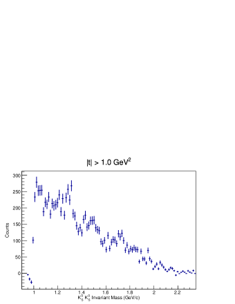
Figure 6: Background subtracted plots for the $4\pi$ invariant mass for $|t|<1$ GeV² (left) and $|t|>1$ GeV² (right).

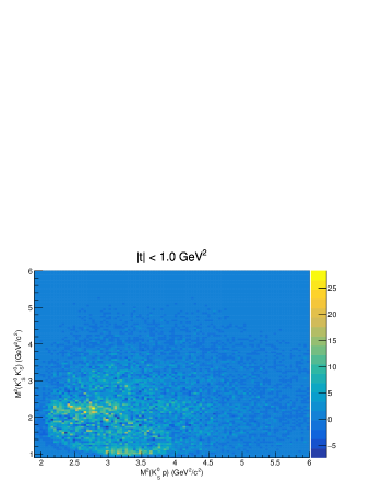
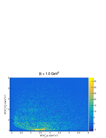
Figure 7: Dalitz plots of the three decay particles, the two kaons and the proton. Structures making horizontal bands represent two-kaon resonances. The intense region at the bottom, near $M^{2}(K_{S}^{0},K_{S}^{0})=1.0$ GeV², is due to the $f_{0}(980)$ decay.

III.2 Dalitz Plots to Look for Baryon Resonances in Background

To look for any possible background baryon resonances decaying into $K_{S}^{0}$ and $p$, Dalitz plots of $M^{2}(K_{S}^{0},K_{S}^{0})$ vs. $M^{2}(K_{S}^{0},p)$, where $M^{2}(X,Y)$ is the squared invariant mass of particles $X$ and $Y$, are plotted in Fig. 7 for $|t|<1$ and $|t|>1$ GeV². These plots include the application of all cuts from Table 1, as well as the momentum transfer cut, and hence are the events remaining in the signal region after sideband subtraction has been done. The sideband subtraction was done on a bin by bin basis.

In Fig. 7, the only structures seen are the horizontal bands, which represent resonances of two $K_{S}^{0}$ mesons. In the $|t|<1$ GeV² plot, the horizontal band at 2.25 GeV² is at the squared mass of the 1.50 GeV peak. Also, the influence of the $f_{0}(980)$ is seen in the $|t|>1$ GeV² plot as a horizontal band near 1 GeV². The lack of any vertical structure indicates that no baryon resonances survive in the sideband-subtracted signal region. Even looking at the Dalitz plots before background subtraction (not shown), no clear vertical structures corresponding to baryon resonances can be seen. This is likely due to the cut on $E_{\gamma^{min}}>2.7$ GeV, which puts the center-of-mass energy, $W$, above the region where any narrow hyperon resonances could be seen.

IV Simulations

IV.1 Modeling the CLAS Detector

In order to study the acceptance of CLAS, $\gamma p\rightarrow K_{S}^{0}K_{S}^{0}p$ events with $K_{S}^{0}K_{S}^{0}\rightarrow\pi^{+}\pi^{-}\pi^{+}\pi^{-}$ were generated isotropically with no dependence on $t$ for the purpose of comparing the data to pure phase space. The incident electron energy was set at 5.7 GeV, which translated into tagged bremsstrahlung photon beam energies of 1.5 GeV to 5.45 GeV. The target was positioned in the simulations exactly as in the g12 run.

These generated events were then passed to a program called GSIM (Geant SIMulation) that models the CLAS detector using GEANT3 libraries, and digitizes the information. After being processed through GSIM, the events are passed through a post processor, which accounted for the condition of the CLAS detector during the g12 experimental run period. Using the g12 run conditions, the post processor removed hits that came from non-functioning parts of the detector and smeared values of measurements depending on the resolution of the corresponding detector element during the g12 run period. These processed events are then fed into the standard CLAS reconstruction software. Details of the reconstruction process are given in Ref. key-12 .

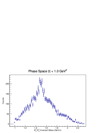
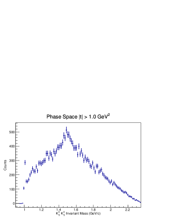
Figure 8: Invariant mass spectrum of $4\pi$ phase space plus simulated $f_{0}(1500)$ and $f_{0}(980)$ mesons decaying to two $K_{S}^{0}$. Momentum transfer cuts $|t|<1$ GeV² (left) and $|t|>1$ GeV² (right) are shown.

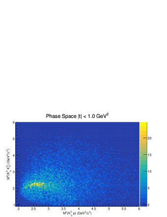
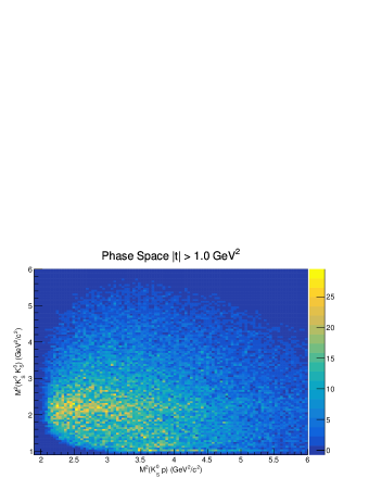
Figure 9: Dalitz plots of simulated events for $M^{2}(K_{S}^{0},K_{S}^{0})$ vs. $M^{2}(K_{S}^{0},p)$ for $|t|<1$ GeV² (left) and $|t|>1$ GeV² (right) for generated phase space plus $f_{0}(980)$ and $f_{0}(1500)$ mesons.

IV.2 Simulations: Phase Space, $f_{0}(980)$ and $f_{0}(1500)$

The Monte Carlo events that passed through the reconstruction software were then fed through the same analysis code as for the real data. The events remaining after this are called accepted events. The upper tail of the $f_{0}(980)$ can decay into two kaons and can be distinctly seen in Fig. 7, in addition to the horizontal band due to the 1.5 GeV resonance. Separate simulations were carried out for $\gamma p\rightarrow f_{0}(980)p$ and $\gamma p\rightarrow f_{0}(1500)p$, and these were then added to the phase space Monte Carlo (MC) events. Cuts were made to divide the simulated four-pion invariant mass spectrum into two sets, one with $|t|<1$ GeV² and the other with $|t|>1$ GeV², as shown in Fig. 8.

The simulated peak at 1.50 GeV, from the $f_{0}(1500)$ decay, is present to a larger extent for $|t|>1$ than for $|t|<1$ GeV². The increased number of counts of the 1.50 GeV peak in the simulations at higher momentum transfer $|t|$ is expected kinematically, due to the increase of the available phase space. This is reiterated in the Dalitz plots shown in Fig. 9. The comparison of the real data with the phase-space MC simulations reinforces the idea that the physical process associated with the production of the peak at 1.50 GeV is from a $t$-channel process.

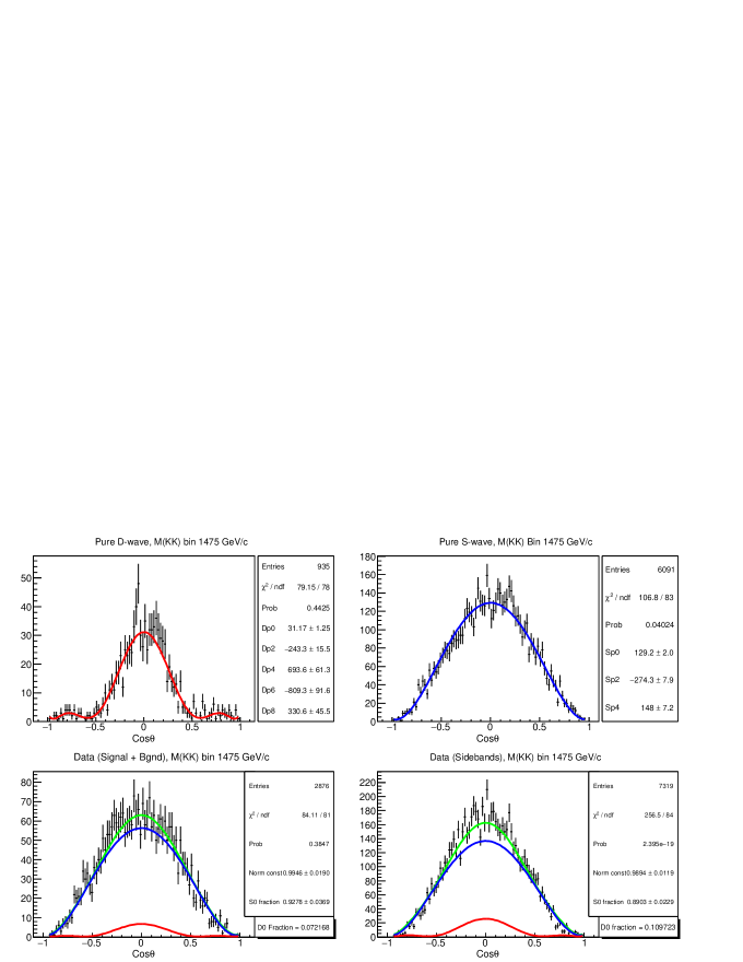
Figure 10: Fits to $\cos\theta_{c.m.}$ distributions in the Gottfied-Jackson frame for simulated pure $S$ wave and pure $D$ wave (top) and data from the S+B and sideband regions (bottom) for bin 1450-1500 MeV of the $K_{S}^{0}K_{S}^{0}$ mass. The fit curves are: $S$ wave (red online), $D$ wave (blue online) and Total (green online). The parameters of the fits are shown to the right of the plots.

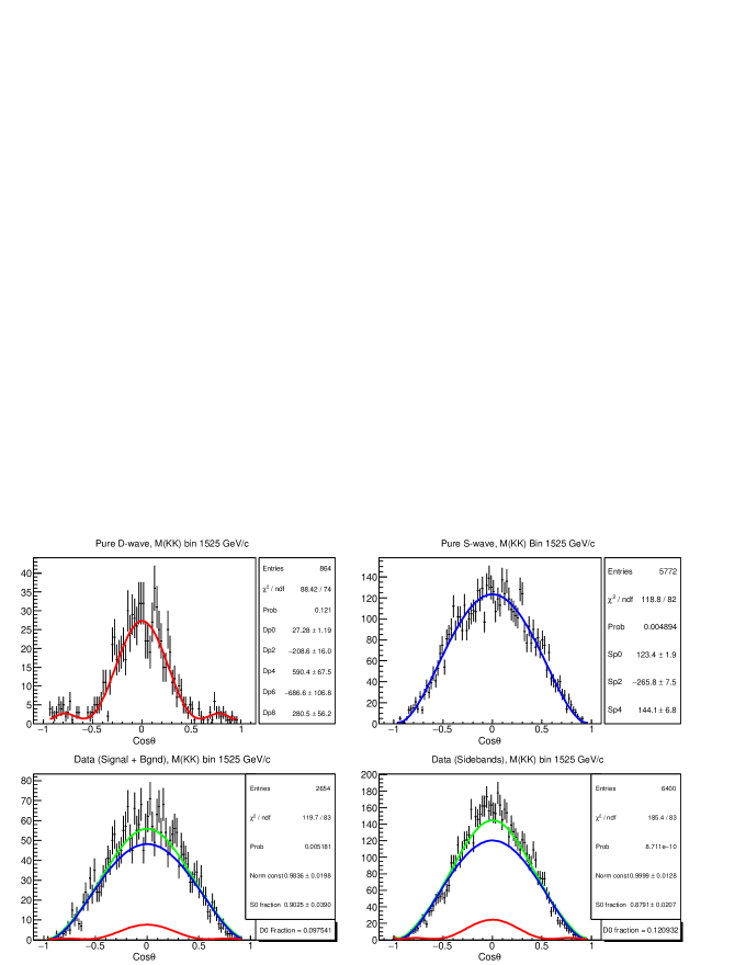
Figure 11: Same as in Fig. 10, but for bin 1500-1550 MeV of the $K_{S}^{0}K_{S}^{0}$ mass.

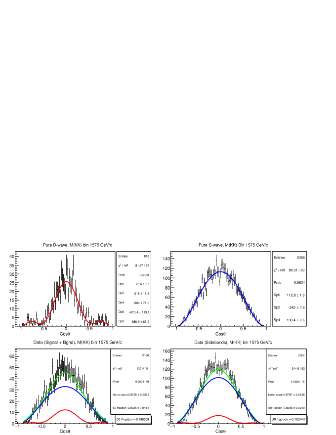
Figure 12: Same as in Fig. 10, but for bin 1550-1600 MeV of the $K_{S}^{0}K_{S}^{0}$ mass.

V Results

In this section, the polar angular distributions of the data and MC are examined in order to extricate the spin contributions from $J=0$ and $J=2$.

The data and Monte Carlo events were binned in 50 MeV intervals of the two-$K_{S}^{0}$ invariant mass. The low statistics of the data do not allow for further binning in $t$ or $E_{\gamma}$ while still providing sufficiently accurate angular distributions. Hence in our analysis of the angular distributions, we examine both the signal + background (S+B) and the sideband background regions, drawing our conclusions based on the comparison of these two regions. The evaluation of the angular distributions of these spectra begins with the generation of simulated pure $S$ and $D$ waves. The phase space distribution behaves like an $S$ wave, so these angular distributions can be obtained by the MC generating phase space. A pure $D$ wave was generated in the Gottfried-Jackson frame and run through the reconstruction software.

Figures 10-12 portray the polar angle distributions (and the fits to it) for the $S$ wave, $D$ wave, data (S+B), and data (sideband) regions for mass bins ranging from 1450-1600 MeV. The polar angle distributions of the simulated pure $S$ and $D$ waves were fit with polynomials including only even orders of $\cos\theta_{c.m.}$ to preserve symmetry. In order to compare these with data, plots of the polar angle in the Gottfried-Jackson frame (after passing through the detector simulations) were normalized such that they have nearly the same number of events as the data.

The distributions of the S+B and sideband regions were fit using the functional shapes extracted from fitting the pure $S$ and $D$ wave angular distributions. The formula used is:

$$Total=N\left(f\cdot(S_{wave})+(1-f)\cdot(D_{wave})\right)\ ,$$ (12)

where $N$ is a normalization constant and $f$ is the fraction of $S$ wave strength. This fitting assumes no interference of $S$ and $D$ waves; in reality we know that interference occurs, but the detector acceptance for CLAS is not uniform and this creates a bi-modal ambiguity in attempts to separate the $S$ and $D$ waves when interference is included in the fits. The above equation provides the most practical indication, within the limitations of the CLAS detector acceptance, of the $S$ and $D$ wave fractions from each mass bin. The lowest (red online) curve denotes the function describing the D-wave, the middle (blue online) one denotes the $S$ wave and the top (green online) curve is the total fit.

Table 2: Fraction of $S$ wave from fits to the S+B and sideband regions.

Mass Bin	$S$ wave fraction	$S$ wave fraction
(MeV)	(S+B region)	(Sidebands)
1000-1050	1.000 $\pm$ 0.045	1.000 $\pm$ 0.031
1050-1100	1.000 $\pm$ 0.031	1.000 $\pm$ 0.029
1100-1150	0.973 $\pm$ 0.025	0.982 $\pm$ 0.018
1150-1200	1.000 $\pm$ 0.023	1.000 $\pm$ 0.015
1200-1250	1.000 $\pm$ 0.022	1.000 $\pm$ 0.011
1250-1300	1.000 $\pm$ 0.013	1.000 $\pm$ 0.063
1300-1350	1.000 $\pm$ 0.020	1.000 $\pm$ 0.011
1350-1400	1.000 $\pm$ 0.028	1.000 $\pm$ 0.026
1400-1450	1.000 $\pm$ 0.025	0.922 $\pm$ 0.019
1450-1500	0.928 $\pm$ 0.037	0.890 $\pm$ 0.023
1500-1550	0.903 $\pm$ 0.039	0.879 $\pm$ 0.021
1550-1600	0.803 $\pm$ 0.044	0.897 $\pm$ 0.024
1600-1650	0.791 $\pm$ 0.056	0.883 $\pm$ 0.032
1650-1700	0.762 $\pm$ 0.052	0.910 $\pm$ 0.031
1700-1750	0.660 $\pm$ 0.053	0.902 $\pm$ 0.033
1750-1800	0.690 $\pm$ 0.071	0.941 $\pm$ 0.041
1800-1850	0.845 $\pm$ 0.086	0.994 $\pm$ 0.096

The values of the fraction of $S$ wave present in the two regions, based on the fits, are tabulated in Table 2. Both the S+B and sideband regions show mostly the shape of a pure $S$ wave up to the 1400 MeV mass bin. In the mass regions 1450-1500 and 1500-1550 MeV, both of which include the peak of interest, the S+B regions have slightly smaller $D$ wave fractions than the corresponding sideband regions, which suggests that the signal is mostly $S$ wave in these mass bins. The higher mass bins (as for the 1550-1600 MeV bin in Fig. 12) involve more $D$ wave shape in the S+B region than in the sidebands, which implies some amount of resonance contributions there. Since there are no well-known $J^{PC}=2^{++}$ resonances in the higher mass bins, we do not speculate as to the possible influence of resonances contributions there. The implications of the peak at 1.50 GeV will be discussed next.

VI Summary and Discussion

In this analysis, the reaction $\gamma p\to pX\to pK_{S}^{0}K_{S}^{0}$ was investigated using data from the g12 experiment at Jefferson Lab. This represents the first high statistics data for photoproduction of scalar mesons with masses above 1 GeV from the CLAS detector. Four charged pions were detected and missing mass was used to identify an exclusive final state. Combinations of $\pi^{+}\pi^{-}$ pairs clearly show correlations from the decay of two $K_{S}^{0}$ over a nearly flat four-pion background. The two identical $K_{S}^{0}$ decay requires the parent meson to have a definite state of $CP=++$.

The sideband-subtraction method was employed to obtain the $K_{S}^{0}K_{S}^{0}$ (or four-pion) invariant mass spectrum, which shows peaks centered at 1.28 GeV and 1.50 GeV, with some background still present. The physics associated with this background is unknown, and examination of Dalitz plots do not show significant background from any narrow hyperon resonances that could reflect into the invariant mass spectrum of the two $K_{S}^{0}$.

At first glance, the resonance at 1.28 GeV could easily be mistaken for the $f_{2}(1270)$. However, the width of the observed peak is much narrower than the average PDG listed width of the $f_{2}(1270)$, so it is not clear if this bump represents a meson resonance or something else (such as a cusp effect). The resonance at 1.50 GeV is distinctly seen at low momentum transfer, but disappears above $|t|>$1 GeV², consistent with production via a $t$-channel process.

The low acceptance at forward and backward angles with CLAS for this final state prevents us from performing a full partial wave analysis. In light of this, to check for contributions from the lowest order symmetric waves, the angular distribution in the Gottfried-Jackson frame of the $K_{S}^{0}K_{S}^{0}$ decay was compared with that of simulated pure $S$ and $D$ waves. Both S+B (signal + background) and sideband regions were separately fit to the decay shape extracted from $S$ and $D$ waves for each $K_{S}^{0}K_{S}^{0}$ mass bin, and differences between the two gave an indication of which partial wave dominates the signal at that mass.

The lower mass bins, from 1000 MeV to 1400 MeV, have almost 100% $S$ wave contribution. For the 1450-1500 and 1500-1550 MeV bins, where the $f_{0}(1500)$ and $f_{2}^{\prime}(1525)$ mesons are expected to contribute, the S+B and sideband regions have similar contributions from $S$ and $D$ waves with slightly larger $S$ wave fractions in the S+B region, suggesting that the signal in this mass range is mostly $S$ wave. However, the assumption of no interference used in the fits (which is a necessary condition due to holes in the CLAS accceptance) prevents a firm conclusion on the $S$ or $D$ wave nature of the peak at 1500 MeV. For bins above 1550 MeV, the $D$ wave fraction in the S+B region is greater than that in the sidebands, implying some $D$ wave in the signal.

In conclusion, fits to the angular distributions of the data suggest that most of the $K_{S}^{0}K_{S}^{0}$ decay in the 1450-1550 MeV mass region is $S$ wave. In addition, the mass and width of the peak at 1500 MeV is consistent with that of the $f_{0}(1500)$. For these reasons, we propose that the observed resonance at 1.50 GeV in Figs. 5 and 6 is most likely from the $S$ wave $f_{0}(1500)\to K_{S}^{0}K_{S}^{0}$. Since this resonance is seen mostly at low momentum transfer ($|t|<1$ GeV²), consistent with $t$-channel meson production, we speculate that the glueball content of this resonance is not large. If confirmed, this result would suggest that the $f_{0}(1710)$ is the more likely candidate to have a high overlap with the lowest glueball state, consistent with recent theoretical indications key-6 .

The $f^{\prime}_{2}(1525)$ has a mass of 1525 MeV and a width of 73 MeV, and hence there is a possibility of it contributing to this mass region in our data. Although the results from the decay angular fits are consistent with the presence of the $f_{0}(1500)$, a contribution from the $f^{\prime}_{2}(1525)$ cannot be ruled out.

This is the first time that this final state has been analyzed in photoproduction and hence it contributes new information to the world data on scalar mesons. Future experiments with the luminosities now available at CLAS12 key-16 and GlueX at Jefferson Lab might afford better statistics and better acceptance for a more definitive study of this final state.

- (1) V. Crede and C. A. Meyer, Prog. Part. Nucl. Phys. 63, 74 (2009).
- (2) C. J. Morningstar and M. Peardon, Phys. Rev. D 60, 034509 (1999).
- (3) J. Beringer et al., (Particle Data Group), Note on scalar mesons below 2 GeV, Phys. Rev. D 88, 0100001 (2012) & revision for the 2015 edition.
- (4) G. ’t Hooft et al., Phys. Lett. B662, 424 (2008).
- (5) F. Giacosa and G. Pagliara, Phys. Rev. C 76, 065204 (2007).
- (6) F. Brünner, D. Parganlija and A. Rebhan, Phys. Rev. D 91, 106002 (2015).
- (7) V. Mathieu, N. Kochelev and V. Vento, arXiv:0810.4453, 2008.
- (8) S. Brodsky, private communication.
- (9) B. A. Mecking et al, Nucl. Instrum. and Meth. A503, 513 (2003).
- (10) D. I. Sober et al., Nucl. Instrum. and Meth. A440, 263 (2000).
- (11) M. D. Mestayer et al., Nucl. Instrum. and Meth. A449, 81 (2000).
- (12) Y. G. Sharabian et al., Nucl. Instrum. Meth. A556, 246 (2006).
- (13) g12 experimental group, CLAS-NOTE 2017-002, https://misportal.jlab.org/ul/Physics/Hall-B/clas/
- (14) E. Pasyuk, CLAS-NOTE 2007-016, https://misportal.jlab.org/ul/Physics/Hall-B/clas/
- (15) S. Stepanyan, arxiv.org:1004.0168.pdf.