Guided Labeling using Convolutional Neural Networks

Abstract

Over the last couple of years, deep learning and especially convolutional neural networks have become one of the work horses of computer vision. One limiting factor for the applicability of supervised deep learning to more areas is the need for large, manually labeled datasets. In this paper we propose an easy to implement method we call guided labeling, which automatically determines which samples from an unlabeled dataset should be labeled. We show that using this procedure, the amount of samples that need to be labeled is reduced considerably in comparison to labeling images arbitrarily.

1 Introduction

Deep learning has gained a lot of interest over the last few years because the methods perform very well on a wide range of machine learning tasks. One class of especially successful deep learning methods are convolutional neural networks (CNNs) for image classification.

Unfortunately, CNNs need a large amount of labeled training data to perform well. In many cases, this labeling is performed by humans. A common approach is to use some form of crowd based labeling. For example, Amazon Mechanical Turk [20] was used for labeling the ImageNet dataset [3]. Data can also be obtained as a side effect of some human interaction with an online system. For example, CAPTCHA [21] challenges to prevent bots using online services can be set up to produce labeled data as a side effect of the verification procedure [5].

Alas, simply labeling all available samples is a very inefficient use of human labor, since not all samples will be of equal value. On the one hand, adding a sample which is similar to samples already in the dataset will not be very usefull. On the other hand, in most cases, not all classes will have the same difficulty and it might make sense to add more samples of the difficult classes to the dataset. Therefore, it would be advantageous to label a sample which would maximize the classification accuracy of a system. Unfortunately, how much the quality of a dataset would increase by adding a specific labeled sample can only be determined after labeling and training on the resulting dataset. This is obviously not useful if we want to decide which samples should be labeled in the first place.

We propose to use the classification confidence of a CNN while trying to predict the class of unlabeled images to decide what to label next. The proposed procedure, together with extensive data augmentation, will be evaluated for two small neural networks on the MNIST [10] and CIFAR10 [9] dataset.

In practice we propose the following workflow: A small, labeled dataset is used to train a neural network that is used to select a batch of the most confusing images from a set of unlabeled data. This batch is given to human workers who label the images, after which they are added to the training dataset and the process repeats. We call this procedure guided labeling. Our hypothesis is that, using this procedure, we are able to trade human for computational resources.

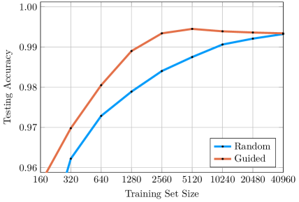
Figure 1: Classification accuracy for the MNIST dataset depending on the size of the training set. It was either randomly sampled from the dataset or generated using the proposed guided labeling approach. Note that the training set size is on a logarithmic scale.

2 Related Work

The idea that a system can decide for itself which data it wants to learn from is generally called active learning. A survey of the field has been published by Settles[15]. The concept of active learning has already been used in 1988 by Angluin [1], although in this case the samples to be labeled were not chosen from a preexisting unlabeled dataset, but synthetically generated by the learner itself. This method is currently not feasible for image classification. Such a method has been shown in 1992 by Baum and Lang [2] to work poorly for handwritten character recognition.

Active learning, where a small amount of labeled data and a larger, fixed set of unlabeled data is available is generally called pool–based sampling as first presented in 1994 by Lewis et al. [11] for learning text classifiers. Pool–based sampling has been used for the task of image classification in 2001 by Tong et al. [19] using support vector machines.

The idea of using the uncertainty of a system to guide the labeling is called uncertainty sampling in the field of active learning and was also already introduced in 1994 by Lewis et al. [11] although they did not use the entropy of a resulting probability distribution as we propose for our method. Entropy as a confusion measure has been used in 2004 by Rebecca Hwa [7] for statistical parsing.

3 Methodology

The following network architectures were used for the experiments. Note that the networks were not selected to give the best possible results for the specific dataset. The important aspect is the difference between the performance on randomly selected images and images selected by guided labeling. All layers, except for the last one, use a ReLU [12] activation function. The last layer uses a softmax activation function.

For the MNIST dataset we employed a network consisting of the following seven layers. Starting from the input layer we have a convolutional layer with 64 $3\times 3$ kernels, a convolutional layer with 128 $3\times 3$ kernels, a max pooling layer with a pooling size of $2\times 2$, a dropout layer [18] with a dropout probability of 0.25, a fully connected layer with 128 output neurons, a dropout layer with a dropout probability of 0.5 and a fully connected layer with 10 output neurons as the last and output layer.

For the CIFAR10 dataset we employ a network consisting of the following eleven layers. A convolutional layer with 32 $3\times 3$ kernels as the input layer, a convolutional layer with 32 $3\times 3$ kernels, a maxpooling layer with a pooling size of $2\times 2$, a dropout layer with a dropout probability of 0.25, a convolutional layer with 64 $3\times 3$ kernels, a convolutional layer with 64 $3\times 3$ kernels, a maxpooling layer with a pooling size $2\times 2$, a dropout layer with a dropout probability of 0.25, a fully connected layer with 512 output neurons, a dropout layer with a dropout probability of 0.5, and a fully connected layer with 10 output neurons as the output layer.

3.1 Data Augmentation

During training, the dataset is randomly augmented for each training epoch. Thus, the network never sees two identical images during training.

For the MNIST dataset, the following augmentations are performed: A rotation in the range $\pm 25\degree$ is applied, the image is scaled in the range $0.8$ to $1.2$, the image is sheared on the X and Y axis in a range of $\pm 20$ pixels, a random elastic distortion as presented by Simard et al. [17] is applied, and the image is cropped back to the original size of $28\times 28$ pixels if necessary.

For the CIFAR10 dataset, the images are randomly mirrored along the vertical axis, are rotated in the range $\pm 25\degree$, are scaled in the range $0.8$ to $1.2$, and are cropped to the original size of $32\times 32$ pixels.

3.2 Measuring Confusion of the Network

Following the work of Park et al. [13] for other machine learning methods, we use the response distribution entropy (RDE) as a classification confidence measure. Feeding a sample through a classification network gives us a probability distribution over all possible classes, which will be called the response distribution. The entropy [16] of this distribution serves as a measure of the overall certainty of the network regarding the classification.

Given a categorical probability distribution with a set of possible classes $C$ and a probability of class $c\in C$ given by $P(c)$, the entropy of this distribution can be calculated by:

$$H(C)=-\sum_{c\in C}P(c)\log_{2}P(c)$$ (1)

If a system predicts a single class with a probability of $1$ this gives us an RDE of $0$ bits. A completely uniform probability distribution over N classes gives us an RDE of $log_{2}|C|$ bits with $|C|$ being the number of classes. Thus, the confidence of a network in the classification decreases with an increasing response distribution entropy.

3.3 Dataset Imbalance

One problem that might arise from generating a dataset by selecting the most confusing samples is that it might become very unbalanced since the most difficult classes will become overrepresented. As shown in the experimental section, this is what happens in practice. We assume that this is, up to a certain point, a beneficial side effect of the guided labeling procedure since we want more samples of confusing classes in our dataset. Unfortunately, extremely unbalanced datasets are problematic when training a neural network. To lessen the effects of imbalance, we weigh misclassifications of underrepresented classes higher in the loss function during training. The weights are calculated in the following fashion:

$$\text{weight}(c)=\max\left(\log\left(\frac{\mu t}{c}\right),1.0\right)$$ (2)

where $t$ is the total number of samples in the training dataset, $c$ is the number of samples for a specific class in the dataset and $\mu$ is a scaling factor which has to be determined empirically. We set $\mu=0.3$ as it provided the best results in our experimental evaluation.

3.4 The Guided Labeling Algorithm

Training starts with a small, labeled training set and a large set of unlabeled images. Depending on the used dataset, one of the convolutional neural networks from section 3 is trained on the training set.

The images of the unlabeled dataset are augmented by the procedure presented in section 3.1. The augmented images are fed into the trained network, which returns class probabilities (i.e. the response distribution). The entropy for this distribution is calculated according to section 3.2, giving us the response distribution entropy for one augmentation of one image. This procedure is repeated multiple times for different augmentations and the average RDE for each image is recorded. This average RDE is an indication for how confusing a certain unlabeled image is for the trained network, also accounting for the employed data augmentation.

A predetermined amount of the most confusing images (the images with the highest average RDE) are selected for labeling. Those images are removed from the unlabeled dataset, labeled by a human, and added to the training set. The CNN is then retrained on this new dataset.

This procedure is repeated until a satisfactory performance is reached, or there is no data left to be labeled. Our hypothesis is that, using this procedure instead of randomly labeling images, satisfactory performance is reached with a dataset containing fewer labeled samples. Algorithm 1 presents pseudo code for the guided labeling procedure.

procedure LabelConfusingSamples($m,X_{u},n$) $\triangleright$ $m$ CNN model, $X_{u}$ unlabeled samples, $n$ # of images to label

     for all $x\in X_{u}$ do

         $R\leftarrow\emptyset$ $\triangleright$ Set to calculate mean RDE for each image

         for $j\leftarrow 1\text{ to }k$ do $\triangleright$ $k$ determines how many augmentations are used for calculating the RDE

              $x_{a}\leftarrow\text{augment}(x)$

              $R\leftarrow R\cup\text{RDE}(m,x_{a})$ $\triangleright$ Get response distribution entropy for augmented sample $x_{u}$ and add to set

         end for

         $r_{x}\leftarrow\text{mean}(R)$ $\triangleright$ Calculate mean RDE for image $x$

     end for

     $X_{l}\leftarrow$ select $n$ samples with highest $r_{x}$

     $Y_{l}\leftarrow$ get labels for $X_{l}$ by manual labeling

     return $X_{l},Y_{l}$

end procedure

procedure GuidedLabeling($X,Y,X_{u}$)$\triangleright$ $X$ samples and $Y$ related labels, $X_{u}$ unlabeled samples

     while achieved accuracy not sufficient $\wedge$ $|X_{u}|\geq|X|$ do

         $m\leftarrow\text{random}()$ $\triangleright$ Randomly Initialize the CNN model

         while model performance still improves on validation dataset do

              $X_{a}\leftarrow\text{augment}(X)$ $\triangleright$ Augment images with random perturbations

              $m\leftarrow\text{trainCNN}(m,X_{a},Y)$ $\triangleright$ Train CNN for one epoch

         end while

         $X_{l},Y_{l}\leftarrow$LabelConfusingSamples($m,X_{u},|X|$) $\triangleright$ $|X|$ = number of samples in $X$

         $X\leftarrow X\cup X_{l},Y\leftarrow Y\cup Y_{l}$ $\triangleright$ Add selected samples to labeled dataset

         $X_{u}\leftarrow X_{u}\backslash X_{l}$ $\triangleright$ Remove selected samples from unlabeled dataset

     end while

     return $X,Y$ $\triangleright$ Return the new labeled dataset

end procedure

Algorithm 1 Guided Labeling Procedure

4 Experimental Evaluation

There are two problems with evaluating the proposed guided labeling method when actually using humans for labeling. First, the procedure is very time consuming and needs a lot of human resources if different modalities have to be tested. Second, it is very hard to decide whether the guided labeling performs better than just randomly labeling images. Because of this, we decided to run the experiments in the following fashion: The network is trained on a small subset of the datasets (MNIST and CIFAR10 respectively) and the remaining images are treaded as being unlabeled. The guided labeling procedure selects images to be labeled, after which they are added to the training set using the labels provided by the dataset.

4.1 Training of the Networks

All our experiments used ADAM [8] as the optimizer with a learning rate of $0.01$ and categorical cross–entropy as the loss function. All weights were initialized using normalized initialization by Glorot et al. [6].

During training, we utilized early stopping, using the accuracy of a validation dataset of $10,000$ images as the stopping criterion. A patience of $100$ epochs was used. This means that if there was no improvement of the accuracy on the validation dataset for $100$ epochs, training was stopped, and the network from $100$ epochs ago is used for testing purposes.

4.2 Selecting the Amount of Images to be Labeled

When using the guided labeling approach, one has to decide how many images should be selected for labeling in each step. In principle, one would expect the method to work better if fewer images are selected in each iteration, since the newly labeled images can be used to inform the selection of images in the next iteration. On the other hand, selecting fewer images results in more iterations. Since for each iteration a neural network has to be trained, the procedure takes longer. In addition, fewer images also means that the labeling workflow including human labor is less efficient. We determined, that an exponential selection scheme offers a good compromise. In the exponential selection scheme, as many images are selected for labeling as are already in the training set. Thus, in every iteration the size of the training set doubles. The number of images to label in iteration $i$ when starting with a labeled training set of size $s$ can be calculated as follows:

$$2^{i-1}s$$ (3)

5 Results

For comparison reasons, identical network architectures are also trained on an equally sized and randomly selected subset of the given dataset. The prediction accuracy of the network trained on images selected using guided labeling and the network trained on randomly selected images is compared on the testing sets provided with the MNIST and CIFAR10 dataset respectively. Prediction accuracy is the number of correctly classified images in relation to the number of tested images.

5.1 MNIST

A comparison of guided labeling using the exponential selection scheme and randomly selected images can be seen in Figure 1 for the MNIST dataset. Note, that the training set size is on a logarithmic scale. It is obvious, that guided labeling is very helpful for MNIST. Not only are we able to achieve the same accuracy with a $16$ times smaller training set ($2,560$ instead of $40,960$ images), but $5,120$ selected images even outperfroms the use of the whole dataset.

An important question is, whether the response distribution entropy of images does actually correlate with samples that would be considered more or less difficult by a human observer. Figure 2 shows the twenty most confusing (highest RDE) and least confusing (lowest RDE) images during the second guided labeling iteration. The most confusing images are clearly difficult images. Many are either unconventional writing styles of numbers, are of poor quality or contain noise. On the other hand, the twenty images with the lowest RDE all show slightly different variations of the number 3 which would probably not add much to the training set, considering that data augmentation is used during training.

(a)

(b) a

(c)

(d) a

Figure 2: The twenty most and least confusing images of the MNIST dataset, selected by the response distribution entropy after two guided labeling steps started on 160 randomly selected images.

One could assume that the number 3 is just in general very distinctive and not confusing for the CNN. To check this we can look at the class distributions in the training set for each guided labeling iteration. This is visualized in Figure 3 in addition to the average class distribution over all iterations, and it shows that the number $3$ seems to be one of the less confusing numbers for the system. Still, overall the MNIST dataset seems to be relatively balanced regarding how confusing different classes are.

(a) Distribution of the images in the training set among the possible classes, for different training set sizes. The training set size is increased using guided labeling. Each doubling in training set size corresponds to one iteration of the guided labeling procedure.

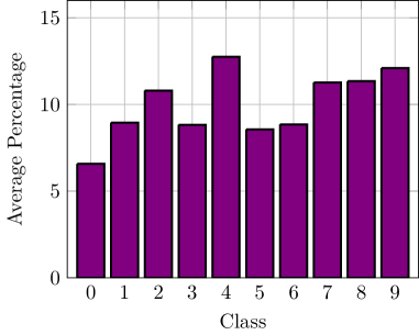
(b) Average distribution of the images in the training set among the possible classes over all training set sizes.

Figure 3: Visualization of the class distribution for different training set sizes for the MNIST dataset. Guided labeling was used to increase the training set size.

5.2 CIFAR10

CIFAR10 seems to be an overall more difficult dataset and the gains from guided labeling are smaller, as can be seen in Figure 4. We give a possible reasons why this may be the case in the discussion. Up until $5,120$ images, guided labeling even performs worse than purely random selection. This presumably happens because up to this point the training set consists of a lot of confusing special cases which do not generalize well to the testing set. After this point, guided labeling performs strictly better than random selection until the training set reaches $40,960$ images, by which point more or less the whole CIFAR10 dataset is used for training. With guided labeling, almost the same performance is reached with $20,480$ images as with using the whole dataset, cutting the amount of images that have to be labeled in half.

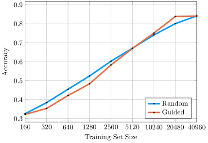
Figure 4: Classification accuracy for the CIFAR10 dataset depending on the size of the training set. It was either randomly sampled from the dataset or generated using the proposed guided labeling approach. Note that the training set size is on a logarithmic scale.

Analogously to the MNIST dataset we also look at the twenty most and least confusing images in Figure 5. The twenty most confusing images are a bit harder to interpred in this case, but compared to the twenty least confusing images a clear difference can be seen. The least confusing images almost exclusively contain bright red cars. Presumably a color that does not appear in images of other classes very often. Compared to the instances of cars in the most confusing images it is obvious that the response distribution entropy does correlate with the difficulty of the images.

(a)

(b) Twenty most confusing images

(c)

(d) Twenty least confusing images

Figure 5: The twenty most and least confusing images of the CIFAR10 dataset, selected by the response distribution entropy after two guided labeling steps started on 160 randomly selected images.

Looking at the class distributions in Figure 6 it is clear that cars are the least confusing class. Presumably because the overall color of the image is already very indicative of this class. It is interesting to note that the technical classes (airplane, automobile, ship, truck) are in general less confusing than the animal classes (especially bird, cat, deer). Looking at the dataset, a lot of the images of technical classes have a very distinct overall appearence (e.g. airplanes usually have sky in the background, ships have water, …). Thus, the training set can become very imbalanced for CIFAR10. The class weights presented in Section 3.3 can mitigate this imbalance to a certain degree.

(a) Distribution of the images in the training set among the possible classes, for different training set sizes. The training set size is increased using guided labeling. Each doubling in training set size corresponds to one iteration of the guided labeling procedure.

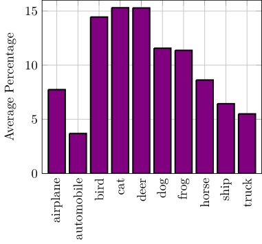
(b) Average distribution of the images in the training set among the possible classes over all training set sizes.

Figure 6: Visualization of the class distribution for different training set sizes for the CIFAR10 dataset. Guided labeling was used to increase the training set size.

6 Discussion

First, we could show that the response distribution entropy is able to identify difficult examples from an unlabeled dataset in case of the MNIST as well as the CIFAR10 dataset. Even when trained on very few images, the response distribution entropy of unlabeled data seems to be a very good metric to detect redundant samples which do not need to be labeled. Second, we demonstrated that the presented guided labeling scheme itself can potentially reduce the number of samples that have to be labeled by a large amount. In case of MNIST a well selected dataset $\frac{1}{16}$ in size achieves the same classification accuracy. For the CIFAR10 dataset the size could still be reduced by one half. Still, why does the procedure perform worse on CIFAR10 than on MNIST? We hypothesize two main reasons. On the one hand, the dataset is much more difficult in general since the classes have much higher variation, which can also not be replicated as easily by augmentation of the images. For example, an image of a bird will always have more variation than an image of the number 7. There is more variation in the background, the lighting, different bird species, etc. On the other hand, the CIFAR10 dataset is also much smaller with respect to the difficulty and therefore less exhaustive. It contains about the same amount of training data as MNIST, despite being much more difficult.

This can also be seen when looking at the achieved accuracy depending on the size of a randomly selected training set. Comparing Figure 1 for MNIST and Figure 4 for CIFAR10, it is apparent that a bigger dataset would likely improve the accuracy for CIFAR10, but would not for MNIST. Going from $20,480$ images to $40,960$ images improved the accuracy by $\approx 4\%$. This is about the same improvement as going from $10,240$ to $20,480$ images. This suggests that increasing the dataset size would likely further improve the achievable accuracy. In case of MNIST, going from $20,480$ images to $40,960$ images only improved the accuracy by $\approx 0.1\%$. So presumably the MNIST dataset is, using augmentation, more or less exhaustive and additional training data would not improve the achievable accuracy significantly.

Presumably, the presented active learning scheme works best if the set of unlabeled data is very big and the achievable accuracy would increase with the size of the unlabeled dataset without increasing the number of samples that actually have to be labeled.

Future research should evaluate the presented method on additional datasets(e.g. CIFAR100 [9], PASCAL [4] and ImageNet [14]). It will also be interesting to see how well a dataset selected using one network architecture will generalize to another architecture. We hypothesized earlier that guided labeling likely would perform better for tasks where a large number of unlabeled data is available. Experiments with synthetically generated dataset, where the amount of unlabeled data is unlimited and labels can easily be generated for each sample, might be able to clarify this. It might also be interesting to bring additional concepts from the field of active learning [15] to the area of deep learning.

7 Conclusion

We presented an active learning method we named guided labeling, that allows for automatic selection of confusing/difficult samples from a pool of unlabeled samples. The method is easy to implement, yet we could show that using it reduces the number of samples needed to achieve a desired accuracy considerably. For MNIST the size of the dataset could be reduced 16 fold, for CIFAR10 it was cut in half. This might move manual labeling to the region of feasibility for some tasks, especially since we hypothesize that results would improve even more if the pool of unlabeled data is very big. In case of the MNIST, the reduced dataset even outperformed training on the full dataset, presumably by removing unnecessary variations that hinder generalizability.

On a more general note, we could show that the field of active learning might have a lot to offer to deep learning practitioners.

References

- [1] D. Angluin. Queries and concept learning. Machine learning, 2(4):319–342, 1988.
- [2] E. B. Baum and K. Lang. Query learning can work poorly when a human oracle is used. In International joint conference on neural networks, volume 8, page 8, 1992.
- [3] J. Deng, W. Dong, R. Socher, L.-J. Li, K. Li, and L. Fei-Fei. Imagenet: A large-scale hierarchical image database. In Computer Vision and Pattern Recognition, 2009. CVPR 2009. IEEE Conference on, pages 248–255. IEEE, 2009.
- [4] M. Everingham, L. Van Gool, C. K. I. Williams, J. Winn, and A. Zisserman. The pascal visual object classes (voc) challenge. International Journal of Computer Vision, 88(2):303–338, June 2010.
- [5] P. Faymonville, K. Wang, J. Miller, and S. Belongie. Captcha-based image labeling on the soylent grid. In Proceedings of the ACM SIGKDD Workshop on Human Computation, pages 46–49. ACM, 2009.
- [6] X. Glorot and Y. Bengio. Understanding the difficulty of training deep feedforward neural networks. In Proceedings of the Thirteenth International Conference on Artificial Intelligence and Statistics, pages 249–256, 2010.
- [7] R. Hwa. Sample selection for statistical parsing. Computational linguistics, 30(3):253–276, 2004.
- [8] D. Kingma and J. Ba. Adam: A method for stochastic optimization. arXiv preprint arXiv:1412.6980, 2014.
- [9] A. Krizhevsky and G. Hinton. Learning multiple layers of features from tiny images. 2009.
- [10] Y. LeCun, L. Bottou, Y. Bengio, and P. Haffner. Gradient-based learning applied to document recognition. Proceedings of the IEEE, 86(11):2278–2324, 1998.
- [11] D. D. Lewis and W. A. Gale. A sequential algorithm for training text classifiers. In Proceedings of the 17th annual international ACM SIGIR conference on Research and development in information retrieval, pages 3–12. Springer-Verlag New York, Inc., 1994.
- [12] V. Nair and G. E. Hinton. Rectified linear units improve restricted boltzmann machines. In Proceedings of the 27th international conference on machine learning (ICML-10), pages 807–814, 2010.
- [13] L. A. Park and S. Simoff. Using entropy as a measure of acceptance for multi-label classification. In International Symposium on Intelligent Data Analysis, pages 217–228. Springer, 2015.
- [14] O. Russakovsky, J. Deng, H. Su, J. Krause, S. Satheesh, S. Ma, Z. Huang, A. Karpathy, A. Khosla, M. Bernstein, A. C. Berg, and L. Fei-Fei. ImageNet Large Scale Visual Recognition Challenge. International Journal of Computer Vision (IJCV), 115(3):211–252, 2015.
- [15] B. Settles. Active learning literature survey. University of Wisconsin, Madison, 52(55-66):11, 2010.
- [16] C. E. Shannon. A mathematical theory of communication. ACM SIGMOBILE Mobile Computing and Communications Review, 5(1):3–55, 2001.
- [17] P. Y. Simard, D. Steinkraus, J. C. Platt, et al. Best practices for convolutional neural networks applied to visual document analysis. In ICDAR, volume 3, pages 958–962, 2003.
- [18] N. Srivastava, G. E. Hinton, A. Krizhevsky, I. Sutskever, and R. Salakhutdinov. Dropout: a simple way to prevent neural networks from overfitting. Journal of machine learning research, 15(1):1929–1958, 2014.
- [19] S. Tong and E. Chang. Support vector machine active learning for image retrieval. In Proceedings of the ninth ACM international conference on Multimedia, pages 107–118. ACM, 2001.
- [20] A. M. Turk. Amazon mechanical turk. Retrieved August, 17:2012, 2012.
- [21] L. Von Ahn, M. Blum, N. J. Hopper, and J. Langford. Captcha: Using hard ai problems for security. In International Conference on the Theory and Applications of Cryptographic Techniques, pages 294–311. Springer, 2003.