Pulsar Rotation Measures and Large-scale Magnetic Field Reversals in the Galactic Disk

Abstract

We present the measurements of Faraday rotation for 477 pulsars observed by the Parkes 64-m radio telescope and the Green Bank 100-m radio telescope. Using these results along with previous measurements for pulsars and extra-galactic sources, we analyse the structure of the large-scale magnetic field in the Galactic disk. Comparison of rotation measures of pulsars in the disk at different distances as well as with rotation measures of background radio sources beyond the disk reveals large-scale reversals of the field directions between spiral arms and interarm regions. We develop a model for the disk magnetic field, which can reproduce not only these reversals but also the distribution of observed rotation measures of background sources.

1 Introduction

Interstellar magnetic fields of our Galaxy have long been known to play fundamental roles in astrophysics and astroparticle physics, and their properties have been investigated for many years. A Galactic magnetic field was proposed by Fermi (1949) as the agent for transport of cosmic rays through interstellar space and, shortly afterward, Kiepenheuer (1950) proposed a synchrotron origin for the Galactic background of radio emission. Remarkably, both Fermi and Kiepenheuer calculated the strength of the interstellar field to be of order a few $\mu$G, very close to current estimates. Magnetic fields contribute significantly to the interstellar hydrodynamic pressure (Boulares & Cox, 1990) and may even be dynamically important in the outer parts of some galaxies (Battaner & Florido, 2007). The strong magnetic fields found in molecular clouds are key to understanding the star-formation process (Rees, 1987). Understanding the structure of the Galactic magnetic field is also important to understanding the origin and maintenance of magnetic fields in other galaxies and in intergalactic space (Beck et al., 1996). For a recent review of Galactic and extragalactic magnetic field observations see Han (2017).

Several tracers have been used to investigate interstellar magnetic fields, including starlight polarization (e.g., Heiles, 1996; Clemens et al., 2012), Zeeman splitting of spectral lines of HI and various molecules (e.g., Crutcher, 1999; Vlemmings, 2008), background synchrotron radiation from our Galaxy (e.g., Beuermann et al., 1985; Bennett et al., 2013; Planck Collaboration et al., 2016a), polarized thermal emission from dust grains in molecular clouds (e.g., Novak et al., 2003; Planck Collaboration et al., 2016b) and Faraday rotation of extragalactic radio sources (EGRS) (Simard-Normandin & Kronberg, 1980; Taylor et al., 2009) and of pulsars (Manchester, 1972; Rand & Lyne, 1994; Han et al., 1999, 2006; Noutsos et al., 2008). These and similar observations have shown that the large-scale magnetic field in galactic disks is largely toroidal and aligned with spiral arm structures, whereas halo fields probably have azimuthal fields with reversed directions above and below the Galactic plane (Han et al., 1997, 1999) though the field scale-height and scale-radius are not yet known. Polarisation observations of synchrotron emission from nearby galaxies suggest that large-scale magnetic fields in galactic disks are predominantly spiral with roughly the same pitch angle both within spiral arms and in interarm regions (e.g. Beck, 2015).

Pulsars are very effective probes of the magnetic field of our Galaxy (Manchester, 1974; Lyne & Smith, 1989; Rand & Kulkarni, 1989; Weisberg et al., 2004; Han et al., 2006). They are highly polarized, have no intrinsic Faraday rotation and are widely distributed throughout the Galaxy at approximately known distances, allowing a three-dimensional tomographic analysis of the field structure. Furthermore, the pulse dispersion gives a unique calibration of the integrated electron density along the line of sight, allowing a direct estimate of the strength of the field:

$$\langle B_{||}\rangle=\frac{\int_{0}^{D}n_{e}{\bf B}.d{\bf l}}{\int_{0}^{D}n_{e}dl}=1.232\frac{\rm RM}{\rm DM},$$ (1)

where $\langle B_{||}\rangle$ is the mean line-of-sight magnetic field component in $\mu$G, weighted by the local electron density $n_{e}$, $D$ is the pulsar distance and RM and DM are respectively the pulsar rotation measure and dispersion measure in their usual units (rad m^-2 and cm^-3 pc). By using pairs of pulsars that are close together on the sky and at distances $D_{1}$ and $D_{2}$ respectively, the mean line-of-sight field component between $D_{1}$ and $D_{2}$ can be obtained from:

$$\langle B_{||}\rangle_{D_{2}-D_{1}}=1.232\frac{\rm RM_{2}-RM_{1}}{\rm DM_{2}-DM_{1}}.$$ (2)

This relation allows analysis of changes in the magnetic field along a given line of sight and hence full tomographic mapping of the Galactic magnetic field. Beck et al. (2003) argued that correlated or anti-correlated electron density with field strength will strongly bias estimates of $B_{||}$, but detailed simulations by Wu et al. (2009, 2015) show this not to be a problem, although the uncertainty of estimated mean field strengths depends on the Mach number of the interstellar medium.

In addition to the field strength, the field directions and their reversals are crucial to the understanding of the structure of Galactic large-scale magnetic fields. Many authors have proposed models for the large-scale structure of the Galactic magnetic field. Based on the RMs of 38 relatively nearby pulsars, Manchester (1974) concluded that the local Galactic magnetic field is basically azimuthal and directed toward longitude $l\sim 90^{\circ}$, that is, clockwise when viewed from the Galactic North Pole. Thomson & Nelson (1980) analyzed RMs of 48 pulsars and found evidence for a field reversal in the inner Carina-Sagittarius arm. After a large number of pulsar RMs were obtained by Hamilton & Lyne (1987), Lyne & Smith (1989) confirmed the first inner reversal and suggested another reversal in the outer Galaxy. Rand & Kulkarni (1989) and Rand & Lyne (1994) fitted concentric ring models to the pulsar RM data with alternating field directions in each ring. Based on more than 350 pulsar RMs, Vallée (2005) revised the ring model to have a dominant clockwise ring field with just one ring of counter-clockwise field in the Galactocentric radius range 5 – 7 kpc. Earlier, both an axisymmetric spiral (ASS) model (Vallée, 1996) and a bisymmetric spiral (BSS) model in which alternate arms have oppositely directed fields (Han & Qiao, 1994; Indrani & Deshpande, 1999; Han et al., 1999) for the global disk magnetic field were suggested, but more recent pulsar RM data do not favour this interpretation (Men et al., 2008). Noutsos et al. (2008) attempted to fit more complex bisymmetric three-dimensional models to pulsar RM data, but the results were inconclusive with none of the tested models giving a good fit to the data.

Radio continuum surveys have enabled measurement of RMs for thousands of EGRS (Taylor et al., 2009), and many authors have used these RMs to constrain models for the large-scale structure of the Galactic magnetic field. Some modelling (Simard-Normandin & Kronberg, 1980; Sofue & Fujimoto, 1983; Pshirkov et al., 2011) favoured a bisymmetric model for the disk field but with only one or two identified field reversals. Most recent models (Brown et al., 2007; Sun et al., 2008; Sun & Reich, 2010; Van Eck et al., 2011; Jansson & Farrar, 2012) with the benefit of a larger sample of EGRS RMs (Brown et al., 2003; Van Eck et al., 2011) are dominated by a general clockwise field but with counterclockwise fields in the Sagittarius/Scutum – Crux spiral zone. Recently, Ordog et al. (2017) used both EGRS and Galactic continuum background data to suggest that the outer boundary of this spiral zone is not perpendicular to the Galactic plane but is sloping toward later longitudes at positive latitudes and earlier longitudes at negative latitudes.

RMs for EGRS are of course integrated along the entire ray path through the Galaxy. They are therefore less sensitive to reversals in the Galactic field direction than pulsars which are distributed throughout the Galaxy. Also EGRS have an intrinsic RM component from Faraday rotation in the host galaxy and also a possible intergalactic component. In analyses of EGRS RMs, these components are generally assumed to be random, just adding to the fluctuations from small-scale variations in the Galactic magnetic field.

Using pulsar RMs, Han et al. (2006) concluded that the data were best represented by a model in which spiral arms have a counter-clockwise field and interarm regions have a clockwise field. This is similar to the BSS models, but with twice as many reversals. This idea has received support from Nota & Katgert (2010) who found evidence from both pulsar and EGRS RMs for a clockwise interarm field between counter-clockwise fields in the Norma and Crux spiral arms.

In the last decade the NE2001 Galactic electron density model (Cordes & Lazio, 2002) has been widely adopted to estimate pulsar distances and also used in modelling of the Galactic magnetic field from EGRS RMs. In this paper, we use the new YMW16 Galactic electron density model (Yao et al., 2017) to estimate pulsar distances from DMs because this model is believed to give more reliable estimates in general (see Table 6 of Yao et al., 2017). Even so, estimated distances to some pulsars can be in error by a factor of two or even more.

Currently there are 732 published pulsar RMs (see Manchester et al., 2005) of which two are for pulsars in the Small Magellanic Clouds, so we have 730 previously published Galactic RMs. There are nearly 2600 Galactic pulsars in the ATNF Catalogue, so there is much scope for new pulsar RM determinations. In this paper, we present measurements made using the Parkes 64-m radio telescope and the Robert C. Byrd Green Bank Telescope (GBT) in several sessions in 2006 and 2007. About 500 pulsars were observed at Parkes in the 20cm band ($\sim$1400 MHz) and about 125 pulsars were observed using the GBT in the 35cm band ($\sim$800 MHz). Analysis of these observations resulted in the determination of RMs for 477 pulsars, of which 441 are either new or more precise than previous measurements. We combine these new measurements with previously published pulsar RMs and with RMs of EGRS to investigate the large-scale structure of the magnetic field in the Galactic disk. Our observations and data reduction methods and the RM samples that we use are described in §2. Details of the analysis for large-scale magnetic fields in different zones of the Galactic disk are given in §3. In §4 we describe a simple model for the Galactic disk magnetic field that is consistent with the Galactic field structures including arm/interarm reversals that we find and with the distribution of EGRS RMs. We conclude the paper in §5 with a brief summary of the main results and the prospects for future work.

2 Observations, data processing methods and the RM samples

2.1 Pulsar observations

We used the Parkes 64-m and the Green Bank 100-m telescopes to observe pulsars that had no previously measured rotation measure (RM) but were sufficiently strong to have a reasonable prospect of measuring a significant RM in one hour or less for Parkes or 15 minutes or less for the Green Bank Telescope (GBT). A few strong pulsars with well-known RMs were also observed at the start of each session as system checks.

The Parkes observations were made in seven sessions between 2006 August 2006 and 2008 February. All observations were in the 20-cm band and, except for one session (2007 March), all used the central beam of the 13-beam multibeam receiver (Staveley-Smith et al., 1996) with a central frequency of 1369 MHz and an observed bandwidth of 256 MHz. For the 2007 March observations the “H-OH” receiver was used with the same bandwidth but at a central frequency of 1433 MHz. Both systems receive orthogonal linear polarisations and have a pulsed calibration signal injected at $45^{\circ}$ to the two feed probes. The system-equivalent flux densities for the two receivers were about 35 Jy and 42 Jy respectively, determined using calibration observations on and off the strong radio source Hydra A, assumed to have a flux density of 43 Jy at 1400 MHz and a spectral index of $-0.91$ (Baars et al., 1977). Multibeam observations were made with half the total observing time at each of two feed angles, $\pm 45^{\circ}$, to reduce the effect of feed cross-coupling on the results. This was not necessary for the H-OH receiver. In the 2006 and 2007 sessions, data were recorded using the PDFB1 signal-processing system; for the two 2008 sessions the PDFB2 system was used. Both systems used a polyphase filterbank and produced mean pulse profiles in 1-minute sub-integrations with full polarisation data in each of 512 frequency channels and with either 512 or 1024 bins across the pulse period. A brief description of these systems is given by Manchester et al. (2013). Data were stored for subsequent analysis as PSRFITS files (Hotan et al., 2004).

The GBT observations were made in 2007 November using the 800 MHz prime focus receiver (see Han et al., 2009, for details) which has a system-equivalent flux density on cold sky of approximately 15 Jy. The Green Bank Astronomy Signal Processor (GASP) pulsar observing system (Demorest, 2007; Ferdman et al., 2004) was used with a central frequency of 774 MHz and a bandwidth of 96 MHz. Flux density calibration was via 3C286 and 3C295, with assumed flux densities at 774 MHz of 19.44 Jy and 35.45 Jy respectively. A polyphase filterbank was used to divide the signal into 4-MHz sub-bands which were distributed to a 16-node computer cluster for real-time coherent dedispersion and additional frequency division to a final resolution of 0.25 MHz. Dedispersed data in each sub-band were then folded in real-time into 1024 pulse phase bins for 30-s sub-integrations and stored using the PSRFITS data format. A 1-min pulsed calibration observation and two 4-min observations at orthogonal feed angles were made for each pulsar.

2.2 Analysis methods for rotation measures

Off-line data analysis including polarimetric calibration and RM determination (see section 2 of Han et al., 2009, for details for GBT observations) was performed using the psrchive pulsar data processing system (Hotan et al., 2004). First, the frequency-time data were examined for radio frequency interference and affected data were excised. Next the data were calibrated to compensate for instrumental gain and phase variations across the band, converted to Stokes parameters and placed on a flux density scale. Where applicable, the two observations at orthogonal feed angles were then summed and the whole observation summed in time. From the resulting multi-frequency polarisation profiles, the RM of each pulsar was obtained as follows. A first guess at the RM was found by searching the range of $\pm 2000$ rad m^-2 for a peak in the total linear polarisation $L=(Q^{2}+U^{2})^{1/2}$ summed across all on-pulse phase bins and across the band, where $Q$ and $U$ are the linear Stokes parameters. This value was then iteratively refined by taking the current best estimate of the RM and summing the data separately in the two halves of the band. A correction to the RM was then obtained from a weighted mean position-angle difference across the pulse profile. Taking the weighted mean difference makes the process relatively immune to orthogonal mode transitions (cf. Ramachandran et al., 2004). The final RM value was then obtained by subtracting the ionospheric RM contribution to give the RM along the path from the top of the ionosphere to the pulsar. The ionospheric RM was computed using a model for the geomagnetic field and the International Reference Ionosphere 2007 (Bilitza & Reinisch, 2008). It was typically between 0.4 to 3.5 rad m^-2 for GBT observations and $-0.2$ to $-2.0$ rad m^-2 for Parkes observations, with a largely diurnal variation.

Table 1: Observed rotation measures for 477 pulsars

PSR Name	Period	DM	Gal. $l$	Gal. $b$	Dist.	RM	$\sigma_{\rm RM}$	Telescope	Obs. Date
	(s)	(cm-3)	(∘)	(∘)	(kpc)	(rad m-2)	(rad m-2)
J0014$+$4746	1.2407	30.85	116.50	$-14.63$	1.78	$-15.3$	0.7	GBT	071119
J0030$+$0451	0.0049	4.33	113.14	$-57.61$	0.36	$16.8$	15.9	PKS	080112
J0034$-$0534	0.0019	13.76	111.49	$-68.07$	1.35	$-38.1$	17.5	PKS	080113
J0034$-$0721	0.9430	11.38	110.42	$-69.81$	1.03	$3.9$	10.4	PKS	080215
J0055$+$5117	2.1152	44.12	123.62	$-11.58$	1.94	$-66.6$	1.5	GBT	071118
J0113$-$7220	0.3259	125.49	300.62	$-44.69$	59.70	$87.0$	28.7	PKS	080111
J0117$+$5914	0.1014	49.42	126.28	$-3.46$	1.77	$-8.1$	6.7	GBT	071118

Note. — Table 1 is published in its entirety in the machine-readable format. A portion is shown here for guidance regarding its form and content.

Table 2: Weighted mean rotation measures

PSR Name	RM	$\sigma_{\rm RM}$	PSR Name	RM	$\sigma_{\rm RM}$
J0437$-$4715	$0.4$	0.2	J1730$-$2304	$-4.9$	1.8
J0656$-$2228	$83.0$	5.4	J1759$-$2302	$1574.7$	13.0
J0815$+$0939	$53.1$	5.0	J1812$-$2102	$322.6$	4.2
J0842$-$4851	$145.1$	11.3	J1816$-$1729	$82.9$	4.1
J0900$-$3144	$82.0$	1.3	J1843$-$0355	$239.7$	9.8
J0902$-$6325	$-59.2$	2.1	J1852$+$0305	$263.9$	14.6
J0942$-$5552	$-63.2$	1.4	J1915$+$0738	$-6.8$	1.5
J0952$-$3839	$331.7$	9.5	J1927$+$1856	$74.4$	5.8
J1032$-$5911	$100.0$	6.7	J1932$+$1059	$-7.5$	0.4
J1626$-$4537	$111.9$	11.2	J2053$-$7200	$15.2$	2.0
J1707$-$4053	$-186.5$	2.5

2.3 Rotation measure samples

Table 1 lists 501 RM measurements for 477 pulsars; for 21 pulsars, repeated observations were made in different sessions, either as a system check or in an attempt to get a better RM measurement. Columns 1 – 6 list the pulsar J2000 name, period, dispersion measure, Galactic longitude, Galactic latitude and the estimated pulsar distance. Unless independent distance estimates are available, distances are based on the YMW16 electron-density model (Yao et al., 2017). The next two columns list the measured RM and its uncertainty, and the final two columns give the telescope and date of the observations. For the pulsars with repeated measurements, we formed weighted mean RMs for use in subsequent analysis. These are listed in Table 2.

The ATNF Pulsar Catalogue (V1.56) lists published RMs for 732 pulsars, of which two are for pulsars that lie in the Small Magellanic Cloud. A total of 91 pulsars in Table 1 have previously published RM measurements and so the total number of available Galactic RMs is 1116. We compare RM values with the previously published values in Table 3. The first two columns give the pulsar J2000 name and the B1950 name if one exists and the next two columns give our best RM measurement from Table 1 or Table 2. The following columns are grouped in sets of three, with the first two columns giving a previously published RM and its quoted uncertainty and the third column giving the reference key for the publication. More recent publications are listed first and reference keys are identified in the Table footnote. Where a reference key for an earlier paper is marked with an asterisk, the corresponding RM measurement is evidently the best available. This applies to 36 of the 91 pulsars and these values are used in subsequent analyses.

Table 3: Comparison of observed rotation measures with previously published values

PSR Name		RM	$\sigma_{\rm RM}$	RM1	$\sigma_{\rm RM_{1}}$	Ref. 1	RM2	$\sigma_{\rm RM_{2}}$	Ref. 2	RM3	$\sigma_{\rm RM_{3}}$	Ref. 3
J0014$+$4746	B0011$+$47	$-15.3$	0.7	$-8.7$	1.1	fdr15
J0034$-$0721	B0031$-$07	$3.9$	10.4	$9.89$	0.07	nsk+15*	$9.8$	0.2	hl87	$10.0$	1.0	man74
J0437$-$4715	$\cdots$	$0.4$	0.2	$1.5$	0.5	nms+97	$0.0$	0.4	ymv+11
J0448$-$2749	$\cdots$	$-0.7$	5.4	$24.0$	17.0	hml+06
J0452$-$1759	B0450$-$18	$12.7$	0.9	$11.1$	0.3	jkk+07*	$13.8$	0.7	hl87	$15.0$	2.0	man74
J0536$-$7543	B0538$-$75	$23.8$	0.9	$25.2$	1.0	njkk08	$28.0$	2.0	hmq99	$21.4$	0.5	qmlg95
J0630$-$2834	B0628$-$28	$45.4$	0.7	$46.5$	0.1	jhv+05*	$46.6$	1.3	hml+06	$45.7$	0.5	vdhm97
J0656$-$2228	$\cdots$	$83.0$	5.4	$38.0$	12.0	njkk08
J0738$-$4042	B0736$-$40	$9.3$	0.9	$12.1$	0.6	njkk08*	$14.5$	0.7	vdhm97	$12.5$	0.6	jkk+07
J0831$-$4406	$\cdots$	$531.4$	22.9	$509.0$	20.0	hml+06
J0835$-$4510	B0833$-$45	$29.9$	0.6	$31.38$	0.01	jhv+05*	$36.6$	0.1	man74	$38.2$	0.1	hmm+77
J0838$-$2621	$\cdots$	$96.3$	12.4	$86.0$	13.0	njkk08
J0843$-$5022	$\cdots$	$189.5$	15.9	$155.0$	23.0	njkk08
J0846$-$3533	B0844$-$35	$136.5$	3.5	$144.0$	8.0	hl87	$159.0$	9.0	qmlg95
J0942$-$5552	B0940$-$55	$-62.8$	1.8	$-61.9$	0.2	tml93*
J0953$+$0755	B0950$+$08	$6.1$	1.6	$-0.66$	0.04	jhv+05*	$2.0$	2.0	hl87	$1.8$	0.5	man74
J1012$+$5307	$\cdots$	$1.0$	1.4	$2.98$	0.06	nsk+15*
J1017$-$5621	B1015$-$56	$332.8$	3.6	$365.0$	7.0	njkk08
J1022$+$1001	$\cdots$	$8.6$	9.5	$1.39$	0.05	nsk+15*	$-0.6$	0.5	ymv+11
J1024$-$0719	$\cdots$	$-5.8$	3.5	$-8.2$	0.8	ymv+11*
J1045$-$4509	$\cdots$	$90.5$	3.5	$92.0$	1.0	ymv+11*	$82.0$	18.0	mh04
J1047$-$3032	$\cdots$	$-26.2$	6.2	$-36.0$	23.0	njkk08
J1052$-$5954	$\cdots$	$-269.7$	11.7	$-280.0$	24.0	wj08
J1054$-$5943	$\cdots$	$150.6$	30.1	$46.0$	34.0	hml+06
J1115$-$6052	$\cdots$	$251.6$	4.6	$257.0$	18.0	wj08
J1156$-$5707	$\cdots$	$228.0$	6.3	$238.0$	19.0	wj08
J1237$-$6725	$\cdots$	$72.5$	21.8	$24.0$	14.0	tjb+13*
J1240$-$4124	B1237$-$41	$17.3$	10.4	$15.0$	13.0	njkk08
J1300$+1$240	B1257+12	$2.3$	3.5	$7.91$	0.06	nsk+15*
J1312$-$6400	$\cdots$	$-12.9$	9.1	$40.0$	30.0	hml+06
J1320$-$3512	$\cdots$	$-4.7$	3.6	$-7.8$	2.0	njkk08*
J1321$+$8323	B1322+83	$-27.5$	1.4	$-23.1$	1.1	fdr15*
J1340$-$6456	B1336$-$64	$-2.1$	20.8	$-37.0$	23.0	njkk08
J1352$-$6803	$\cdots$	$20.4$	2.4	$30.0$	7.0	njkk08
J1403$-$7646	$\cdots$	$63.4$	17.3	$94.0$	16.0	njkk08*
J1514$-$4834	B1510$-$48	$13.8$	18.2	$18.0$	14.0	njkk08*
J1524$-$5625	$\cdots$	$185.8$	3.3	$180.0$	20.0	wj08
J1524$-$5706	$\cdots$	$-475.5$	5.0	$-470.0$	20.0	wj08
J1534$-$5405	B1530$-$53	$-86.8$	6.0	$-69.0$	12.0	njkk08
J1600$-$3053	$\cdots$	$-11.9$	3.7	$-15.5$	1.0	ymv+11*
J1614$-$3937	$\cdots$	$84.0$	13.7	$133.0$	16.0	njkk08
J1615$-$5537	B1611$-$55	$10.2$	14.8	$-54.0$	16.0	njkk08
J1623$-$4256	B1620$-$42	$109.6$	5.7	$-15.0$	8.0	hml+06
J1628$-$4804	$\cdots$	$-447.0$	15.5	$-431.0$	43.0	hml+06
J1644$-$4559	B1641$-$45	$-626.9$	0.8	$-617.0$	1.0	hml+06	$-611.0$	2.0	vdhm97
J1650$-$1654	$\cdots$	$16.1$	5.6	$7.0$	14.0	njkk08
J1651$-$4246	B1648$-$42	$-167.4$	1.1	$-154.0$	5.0	hml+06
J1702$-$4128	$\cdots$	$-165.5$	4.7	$-160.0$	20.0	wj08
J1705$-$3950	$\cdots$	$-98.8$	1.9	$-106.0$	14.0	wj08
J1707$-$4053	B1703$-$40	$-183.7$	3.4	$168.0$	4.0	njkk08	$-207.0$	25.0	qmlg95
J1709$-$4429	B1706$-$44	$-3.5$	0.8	$0.70$	0.07	jhv+05*	$-7.0$	4.0	qmlg95
J1713$+$0747	$\cdots$	$7.0$	7.6	$8.4$	0.6	ymv+11*
J1717$-$4054	B1713$-$40	$-811.4$	4.1	$-800.0$	100.0	khs+14
J1721$-$3532	B1718$-$35	$148.1$	5.9	$159.0$	4.0	njkk08*	$205.0$	75.0	qmlg95
J1730$-$2304	$\cdots$	$-4.9$	1.8	$-7.2$	2.2	ymv+11
J1737$-$3137	$\cdots$	$449.6$	5.1	$448.0$	17.0	wj08
J1737$-$3555	B1734$-$35	$68.6$	9.8	$50.0$	4.0	njkk08*
J1744$-$1134	$\cdots$	$6.0$	2.1	$-1.6$	0.7	ymv+11*
J1818$-$1422	B1815$-$14	$1173.9$	7.3	$1168.0$	13.0	hml+06
J1822$-$4209	$\cdots$	$40.7$	10.6	$-13.0$	9.0	hml+06
J1828$-$1101	$\cdots$	$59.4$	2.5	$45.0$	20.0	wj08
J1835$-$0643	B1832$-$06	$44.1$	14.6	$62.0$	38.0	hml+06
J1835$-$1106	$\cdots$	$42.9$	2.1	$42.0$	3.0	njkk08
J1836$-$1008	B1834$-$10	$826.6$	4.5	$-1000.0$	99.0	hl87
J1837$-$0045	$\cdots$	$131.6$	6.7	$130.0$	17.0	njkk08
J1837$-$0604	$\cdots$	$320.8$	4.2	$450.0$	25.0	wj08
J1837$-$1837	$\cdots$	$137.2$	9.0	$138.0$	8.0	njkk08*
J1841$-$0345	$\cdots$	$450.5$	2.6	$447.0$	15.0	wj08
J1845$-$0743	$\cdots$	$448.4$	1.8	$440.0$	12.0	wj08
J1853$-$0004	$\cdots$	$648.7$	4.7	$647.0$	16.0	wj08
J1900$-$2600	B1857$-$26	$-9.3$	0.2	$-2.3$	0.8	jhv+05	$-7.3$	0.8	hl87
J1900$-$7951	B1851$-$79	$18.6$	5.4	$43.0$	12.0	qmlg95
J1901$-$1740	$\cdots$	$-20.0$	8.7	$63.0$	33.0	njkk08
J1903$+$0135	B1900$+$01	$68.4$	2.4	$72.3$	1.0	hl87*
J1915$+$1606	B1913$+$16	$364.5$	5.0	$430.0$	73.0	hml+06
J1917$+$2224	B1915$+$22	$168.2$	23.5	$192.0$	49.0	wck+04
J1919$+$0134	$\cdots$	$44.8$	18.2	$47.0$	4.0	njkk08*
J1921$+$1419	B1919+14	$164.8$	3.1	$275.0$	60.0	hr10
J1926$+$0431	B1923$+$04	$-39.5$	8.1	$0.0$	11.0	hl87
J1932$+$1059	B1929$+$10	$-8.2$	0.8	$-6.87$	0.02	jhv+05*	$-7.0$	2.0	hl87	$-8.6$	1.8	man74
J1932$-$3655	$\cdots$	$3.8$	4.7	$-8.0$	3.0	njkk08*	$-6.0$	3.0	hmq99
J1935$+$1616	B1933$+$16	$-2.3$	0.5	$-10.2$	0.3	jhv+05	$-2.0$	2.0	hl87	$-1.9$	0.4	man74
J1943$-$1237	B1940$-$12	$-75.4$	6.2	$-10.0$	8.0	hl87
J1949$-$2524	B1946$-$25	$-51.9$	13.8	$-13.0$	8.0	hmq99
J2038$-$3816	$\cdots$	$20.5$	9.5	$38.0$	14.0	njkk08	$68.0$	18.0	hml+06
J2048$-$1616	B2045$-$16	$-9.7$	1.7	$-10.0$	0.3	jkk+07*	$-9.0$	2.0	hl87	$-10.8$	0.4	man74
J2053$-$7200	B2048$-$72	$15.0$	2.0	$17.0$	1.0	qmlg95*
J2108$-$3429	$\cdots$	$93.1$	8.9	$39.0$	12.0	njkk08	$50.0$	20.0	hmq99
J2155$-$3118	B2152$-$31	$33.8$	14.4	$21.0$	3.0	hl87*
J2324$-$6054	B2321$-$61	$15.6$	2.0	$-11.0$	8.0	hml+06	$39.0$	6.0	qmlg95
All RM values and their uncertainties are in units of rad m-2. References marked with * signify the best available RM values if not from the present work. References: fdr15: Force et al. (2015); hl87: Hamilton & Lyne (1987); hml+06: Han et al. (2006); hmm+77: Hamilton et al. (1977); hmq99: Han et al. (1999); hr10: Hankins & Rankin (2010); jhv+05: Johnston et al. (2005); jkk+07: Johnston et al. (2007); khs+14: Kerr et al. (2014); man74: Manchester (1974); mh04: Manchester & Han (2004); njkk08: Noutsos et al. (2008); nms+97: Navarro et al. (1997); nsk+15: Noutsos et al. (2015); qmlg95: Qiao et al. (1995); tjb+13: Tiburzi et al. (2013); tml93: Taylor et al. (1993); vdhm97: van Ommen et al. (1997); wck+04: Weisberg et al. (2004); wj08: Weltevrede & Johnston (2008); ymv+11: Yan et al. (2011)

Most of the new measurements are in good agreement with previously published values with only ten cases where the RM difference exceeds five times the combined uncertainty. Some of the smaller differences are likely to result from temporal variations of the RM as seen in, for example, the Vela pulsar (Hamilton et al., 1985). Four of the measurements are discrepant by more than $10\sigma$. The largest of these discrepencies is for PSR J1707$-$4053 where our measured RM is $-183.7\pm 3.4$ rad m^-2 compared to $+168.0\pm 4.0$ rad m^-2 from Noutsos et al. (2008). Our measurement agrees well with a more recent measurement by Force et al. (2015) and with an older measurement by Qiao et al. (1995) and so it appears that the Noutsos et al. (2008) measurement is incorrect. The other three cases are PSRs J1623$-$4256, J1836$-$1008 and J1935+1616. Previous observations for PSR J1623$-$4256 (Han et al., 2006) unfortunately were processed with an incorrect DM; re-analysis of these data with the correct DM gives an RM consistent with that presented here. For PSR J1836$-$1008, the new RM in Table 1 is confirmed by analysis of more recent data. For PSR J1935+1616, the new measurement agrees with two previous determinations, so it appears that the Johnston et al. (2005) result is discrepant. Among the 1116 Galactic pulsars with RMs, 787 are at low Galactic latitudes ($|b|<8^{\circ}$) and hence most relevant to the present work.

We also make use of 3933 RMs of extragalactic radio sources (EGRS) with Galactic latitude $|b|<8^{\circ}$ (Xu & Han, 2014). Of these, 2942 are from the analysis of NVSS data by Taylor et al. (2009), 283 from Brown et al. (2003), 184 from Van Eck et al. (2011), and 104 from Brown et al. (2007). The remaining 298 RMs are from a variety of papers.

3 Large-scale field structure in the Galactic disk

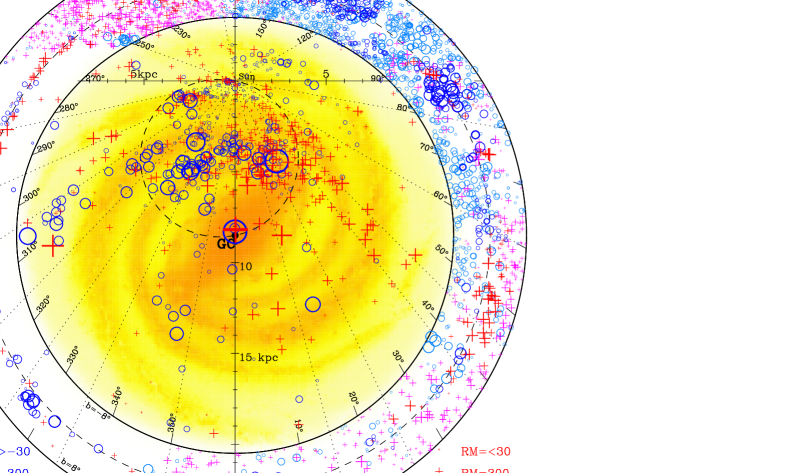
Figure 1: Distribution of pulsars and EGRS with measured RMs in Galactic coordinates. The central part of the figure shows RMs for pulsars with Galactic latitude $|b|<8^{\circ}$ projected on to the Galactic disk and the outer ring shows the distribution of RMs for EGRS with $|b|<8^{\circ}$. Radial distance in the outer ring is linearly proportional to Galactic latitude. The light blue and pink symbols indicate the RMs derived from NVSS data (Taylor et al., 2009). Blue circles and red + signs in both central part and the outer ring indicate negative and positive RMs respectively and the symbol size is proportional to $|RM|^{1/2}$. The background in the central part of the figure is an artist’s impression of the Galactic structure modified from a NASA/JPL image (Credit: R. Hurt) according to updated spiral arms of Hou & Han (2014). The dashed circle gives the locus of tangent points assuming a spiral pitch angle of $11^{\circ}$ and the dotted lines give the longitude boundaries of the approximately tangential spiral-arm or interarm zones and anti-center zones used for the RM analyses in this paper.

Figure 1 shows the overall RM distribution for both pulsars and EGRS within $8^{\circ}$ of the Galactic plane. In general terms, there is predominance of positive RMs in the first and third Galactic quadrants (i.e., $0^{\circ}<l<90^{\circ}$ and $180^{\circ}<l<270^{\circ}$) and of negative RMs in the other two quadrants. Since positive RMs indicate fields directed toward us, overall these results suggest clockwise fields in the outer Galaxy and counterclockwise fields inside the Sun viewed from the north Galactic pole. At least in the first and fourth quadrants, there is a tendency for more distant pulsars to have larger RMs, indicating the large scale of the counter-clockwise fields in the inner Galaxy.

Closer examination of Figure 1 shows however that this counter-clockwise field in the inner Galaxy is predominantly confined to the spiral arms. This is most clearly revealed by increasingly negative RMs in the vicinity of spiral-arm tangential points, for example, the Crux tangential region near Galactic longitude $l\sim 310^{\circ}$ and the Norma tangential region near Galactic longitude $l\sim 330^{\circ}$. In contrast, in the interarm tangential regions, for example, in the Norma-Crux interarm region near $l\sim 320^{\circ}$ and the Crux-Carina interarm region ($l\sim 300^{\circ}$), RMs are positive, indicating a clockwise field similar to the local interarm region. Furthermore, EGRS RMs in the direction around the Crux-Carina interarm region ($l\sim 300^{\circ}$) are nearly all large and positive, confirming the large-scale clockwise field. In the first quadrant, the counter-clockwise fields in the spiral arms are generally clear, but it is difficult to identify the direction of the interarm fields since the spiral arms are much closer and less well defined in this quadrant.

In the following sub-sections, we quantify these RM trends by fitting the observed variations of RM with DM and distance over specified distance ranges and directions and comparing these fits with the mean EGRS RM in the same direction. As discussed in §1, we can use Equation 2 to give the mean line-of-sight component of the interstellar magnetic field, weighted by the local $n_{e}$, over different distance intervals along the line of sight to pulsars in similar directions. Distances to individual pulsars derived from Galactic $n_{e}$ models are subject to unpredictable errors. Therefore, rather than fitting to pulsar pairs individually, we fit linear trend lines to plots of RM vs distance over specified distance intervals and to plots of RM vs DM over DM intervals that match the distance range as closely as possible. The averaging over groups of pulsars minimises the effects of small-scale B-field fluctuations and distance errors. We emphasize that the derived B-field estimates are derived solely from the RM – DM fits.

In order to improve the reliability of the $B$-field estimates, we omitted RMs of 15 pulsars with an uncertainty larger than 35 rad m^-2 and used the Maximum Likelihood Robust Estimate routine from Press et al. (1996, see pp.694-700) to fit a line by minimizing absolute deviation (i.e. the medfit subroutine). This “robust” fitting is necessary so that outliers resulting from HII regions, other unmodelled electron-density fluctuations or magnetic-field fluctuations along the path do not unduly influence the slope of the fitted line. We take as the uncertainty of the slope the mean absolute deviation of RMs from the fitted line divided by the DM range for the fitting. Generally, the scatter around the fitted lines in the RM – DM plots is dominated by real fluctuations in the line-of-sight magnetic field components, not RM measurement errors which are very small compared to the data scatter. Positive slopes of RM vs DM correspond to magnetic fields directed toward us, i.e., to clockwise fields in the Galactic Quadrant 4 and counter-clockwise fields in the Galactic Quadrant 1.

The regions for which we have analysed the RMs are listed in Table 4. The arm and interarm designations are guided by the 4-arm spiral model of Hou & Han (2014, i.e. the background images of Fig. 1), and the ranges for the Galactic longitude $l$ are chosen accordingly. For the inner Galactic quadrants, the fitted regions are guided by the tangential zones since spiral fields have a small angle to our line of sight and distance errors have less effect there. However, where clear trends in RM versus DM or distance exist, the fitted region has been adjusted to encompass these. For the outer Galactic regions, the fitted regions are determined by the RM trends. The fifth column of Table 4 gives the number of pulsars in the fitted region or the number of EGRS for each longitude range. The next two columns give estimates of $B_{||}$ and field direction from the RM – DM fits in the vicinity of tangential regions of Quadrants 1 and 4. Comparison of the RMs of background EGRS with the RMs of the most distant pulsars in each zone gives a good indication of the magnetic field orientation beyond the pulsars, but it is not possible to reliably estimate field strengths in these cases because of the uncertain DM contribution.

Table 4: Galactic disk zones and their magnetic fields

Region	$l$–Range	D–Range	DM–Range	No. PSRs	$B_{||}$	B-field	Arrow $l$		Arrow D
	(∘)	(kpc)	(cm-3 pc)	or EGRS	($\mu$G)	Direction	(∘)		(kpc)
Quadrant 1
Near 3-kpc	15 – 25	3.5 – 6.5	350 – 850	25	$+4.0\pm 0.7$	ccw	20	5.5
Near 3-kpc – EGRS	15 – 25	6.5 – E	850 – E	71		cw	20	11.0
Scutum	25 – 38	4.0 – 8.0	200 – 800	46	$+0.4\pm 0.4$	ccw	32	7.0
Scutum – EGRS	25 – 38	9.5 – E	900 – E	78		–	–	–
Scutum – Sgr	38 – 45	4.0 – 12.0	200 – 500	25	$+3.3\pm 0.9$	ccw	42	8.5
Scutum-Sgr – EGRS	38 – 45	12.0 – E	500 – E	37		cw	42	13.0
Sagittarius	45 – 60	3.0 – 8.5	100 – 300	30	$+1.4\pm 1.0$	ccw	50	5.0
Sagittarius – EGRS	45 – 60	8.5 – E	300 – E	176		cw	50	8.5
Local – Perseus	60 – 80	3.5 – 8.0	70 – 250	14	$+0.7\pm 0.7$	ccw	73	7.0
Local–Perseus – EGRS	60 – 80	8.0 – E	250 – E	225		cw	73	10.5
Outer Zones for the local region and the Perseus arm
Local Q1-Q2	80 – 120	1.0 – 5.0	10 – 200	18	$-1.4\pm 0.6$	cw	105	2.5
Local Q1-Q2 – EGRS	80 – 120	5.0 – E	200 – E	576		ccw	105	4.0
Outer Q2	120 – 190	–	–			–	–	–
Outer Q3	190 – 250	0.0 – 3.5	0 – 130	13	$+1.3\pm 0.4$	cw	235	2
Outer Q3 – EGRS	190 – 250	3.5 – E	130 – E	841		ccw	230	3.5
Local Q3-Q4	250 – 270	0.0 – 6.0	30 – 280	20	$+1.1\pm 0.5$	cw	260	4.0
Local Q3-Q4 – EGRS	250 – 270	6.0 – E	280 – E	138		ccw	260	6.5
Outer Carina	270 – 282	0.1 – 1.1	50 – 250	23	$+0.8\pm 0.5$	cw	276	0.7
Outer Carina – EGRS	270 – 282	–	250 – E	26		ccw	276	9.0
Quadrant 4
Carina	282 – 294	2.0 – 4.0	250 – 550	22	$-1.2\pm 1.0$	ccw	288	3.0
Carina – EGRS	282 – 294	4.0 – E	550 – E	8		cw	288	11.0
Carina – Crux	294 – 304	2.0 – 10.0	100 – 600	21	$+1.9\pm 0.3$	cw	299	7.0
Carina–Crux – EGRS	294 – 304	10.0 – E	600 – E	13		ccw	299	12.0
Crux	304 – 316	4.0 – 13.0	200 – 800	38	$-1.6\pm 0.5$	ccw	310	7.5
Crux – EGRS	304 – 316	13.0 – E	800 – E	13		cw	310	13.0
Crux – Norma	316 – 325	3.0 – 11.0	250 – 700	9	$+1.3\pm 0.3$	cw	320	6.0
Crux-Norma – EGRS	316 – 325	11.0 – E	700 – E	6		ccw	320	12.0
Norma	325 – 335	4.0 – 6.5	300 – 800	15	$-3.7\pm 0.6$	ccw	330	6.5
Norma – EGRS	325 – 335	10.0 – E	900 – E	20		cw	330	12.5
Far 3-kpc	335 – 350	8.0 – 13.5	400 – 700	23	$-3.1\pm 1.1$	ccw	343	12.5
Far 3-kpc – EGRS	335 – 350	13.5 – E	700 – E	23		cw	343	15.5

3.1 Fourth Galactic Quadrant

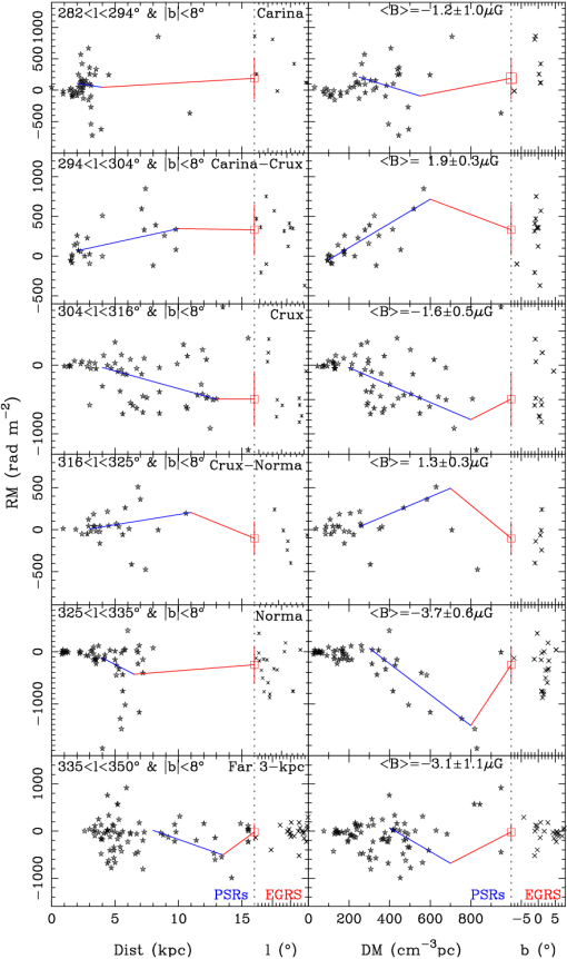
Figure 2: RMs for pulsars versus pulsar distance and DM and RMs for EGRS versus Galactic longitude (left panels, scale ticks are given but not labelled) and Galactic latitude (right panels) for arm and interarm regions in the fourth Galactic quadrant. The blue lines represent linear fits to the pulsar RM gradients, primarily in the tangential regions. For the RM – DM case, the slope of this line gives the mean interstellar line-of-sight magnetic field in the region with positive slopes corresponding to clockwise fields. The red square and error bar represent the median and rms deviation from the median of the RMs of EGRS in the region. Uncertainties in the measured RMs are plotted but are generally smaller than the plotted symbol size.

We discuss Quadrant 4 first since, as viewed from the Earth, the Galactic spiral arm and interarm regions are more clearly separated than they are in Quadrant 1. Figure 2 shows the Quadrant 4 pulsar RMs as functions of distance and DM and EGRS RMs as a function of Galactic latitude or longitude for the longitude ranges given in Table 4.

From the top subpanels down, Figure 2 shows alternating interarm and arm regions (cf. Table 4). It is striking that the field directions alternate in the tangential regions, that is, the RM – DM slope is generally negative in arm regions, corresponding to counter-clockwise field directions, but positive in interarm regions, corresponding to clockwise field directions.

Despite the fact that there are few known pulsars beyond the tangential zones, comparison of RMs for distant pulsars with EGRS RMs (Figure 2) clearly shows that for all of these longitude zones there are field reversals beyond the tangential regions. For example, at the far end of the Norma tangential region (325^∘$<l<$ 335^∘) pulsar RMs are very negative (as much as $\sim-1500$ rad m^-2) whereas RMs of EGRS in this direction have a much smaller median RM of about $-200$ rad m^-2. This implies at least one field reversal along this line of sight.

Similar distant reversals are seen for most of the other arm and interarm regions. It is not possible to say exactly where these reversals occur because of large uncertainties in the pulsar distances, although they definitely occur beyond the fitted regions. Since both the magnetic field strength and the electron density have a general decline with increasing Galactocentric radius and, at least in Quadrants 1 & 4, the field makes a greater angle with the line of sight beyond the tangential point, it is reasonable to assume that the most significant zone affecting the gradient in the RMs of Galactic – EGRS is centered on the extension of the next outer arm/interarm region. For example, the Norma – EGRS reversed field probably results from the extension of the clockwise fields found in the tangential zone of the Crux – Norma interarm region (316^∘$<l<$325^∘). The Crux – Norma interarm zone itself appears to show a reversal between the end of the tangential region and the edge of the Galaxy, probably due to counter-clockwise fields in the distant Crux arm. Similar considerations apply to the 3-kpc, Crux, Carina – Crux and Carina zones although the evidence is generally somewhat weaker compared to the Norma – Crux zones. Table 4 lists the derived field strengths and directions, quantifying these field reversals.

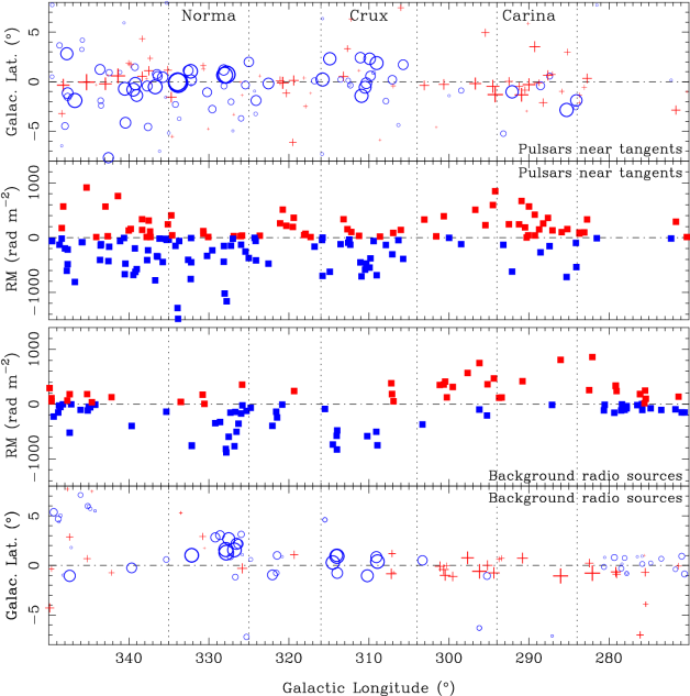
Figure 3: RMs for pulsars in the tangential zone ($\pm 50\%$ from the tangent trajectory, considering the large uncertainty of pulsar distances) and RMs for EGRS versus Galactic longitude in the fourth Galactic quadrant. The top and bottom panels show their distribution in Galactic latitude of the pulsars and the EGRS respectively with the symbol size proportional to RM^1/2.

These reversals are further illustrated by Figure 3 which shows the RM distributions for pulsars in the tangential zones and for the EGRS. The pulsar RMs (second panel) show a clear alternating structure between arm and interarm regions at least up to the Carina region ($l<294^{\circ}$) with arm regions (Crux, $l\sim 310^{\circ}$ and Norma, $l\sim 330^{\circ}$) predominently negative (corresponding to counter-clockwise fields) and interarm regions predominently positive (clockwise fields). The RMs of EGRS do not show these alternative reversals as clearly as pulsar RMs, especially in the interarm regions.

The derived field strengths and directions are illustrated in Figure 4 where the arrows are placed at the approximate mean distance for the relevant RM – DM fit for the pulsars and near the next spiral feature for the pulsar – EGRS fields as listed in Table 4. As discussed above, there is substantial distance uncertainty in both cases, but in general, the derived field directions are consistent with reversals between the arm and interarm regions. Arrow locations are listed in the final two columns of Table 4.

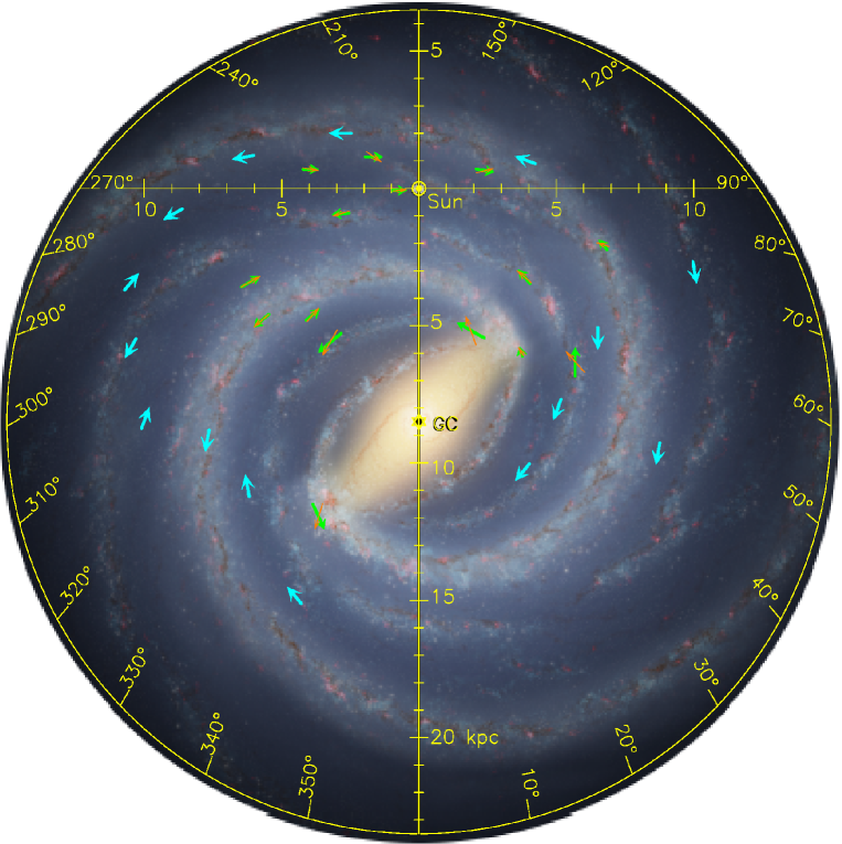
Figure 4: Large-scale magnetic field directions in the Galactic disk, derived from the fitted gradients of pulsar RMs with DM/distance and the comparison of RMs of EGRS with RMs of distant pulsars. The orange arrows give the derived line-of-sight magnetic field components and the green arrows show the inferred spiral field. For both of these, the arrow length is proportional to the square root of the field strength. The blue arrows, which are all of the same length, give the inferred spiral field direction derived from the comparison of RMs for EGRS with RMs for distant pulsars and are placed at the distance of the central axis of the next outer spiral feature (arm or interarm). The background image shows an artist’s impression of the structure of our Galaxy from a NASA/JPL image (Credit: R. Hurt) modified according to the spiral structure of Hou & Han (2014).

3.2 First Galactic Quadrant

RMs in Quadrant 1 are generally positive (see Figure 1) and there is a much less clear delineation between the arm and interarm regions compared to Quadrant 4. Many authors have described the positive and increasing RMs in the Sagittarius arm, implying a counter-clockwise field in this arm (e.g., Lyne & Smith, 1989; Rand & Lyne, 1994; Han & Qiao, 1994; Indrani & Deshpande, 1999; Weisberg et al., 2004). Figure 5 shows positive RMs increasing with distance and DM in Sagittarius tangential region (45^∘$<l<$ 60^∘). The Sagittarius arm becomes the Carina arm in Quadrant 4, supporting the idea that Carina fields conform to the counter-clockwise pattern.

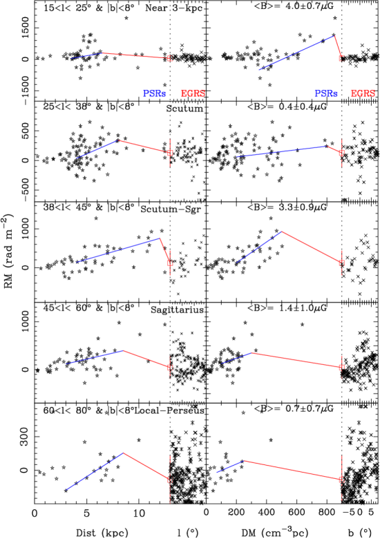
Figure 5: Same as Fig. 2 but for RMs for pulsars and EGRS in the first Galactic quadrant. Positive slopes in the RM – DM plots indicate counter-clockwise fields.

However, fields in the nominal Scutum – Sagittarius interarm region (38^∘$<l<$ 45^∘) show an even clearer positive and increasing pattern, implying counter-clockwise fields in this region also. A possible explanation for this is that these fields originate in more distant parts (up to 12 kpc, including both the Sagittarius arm and the Perseus arm). However, the RMs of EGRS are much smaller on average, indicating the field reversals beyond these spiral arms. Positive and increasing RMs are also seen in the Near 3-kpc region (15^∘$<l<$ 25^∘) which could result from the inner part of the Norma arm.

Beyond the interarm region with clockwise magnetic fields, the RM change to positive for distant pulsars ($D>5$ kpc) in the longitude range of 60^∘$<l<$ 80^∘in Figure 5 shows some evidence for counter-clockwise fields in the Perseus arm. The small RMs of EGRS in this direction indicate another field reversal beyond the Perseus arm. The counter-clockwise field in the Perseus arm is echoed by the RM difference of pulsars in the outer Galaxy nearer than or within the arm and the RMs of EGRS, as we will see below.

As in Quadrant 4, there is evidence for reversals beyond the tangential regions based on the mean RMs of EGRS, at least for the Scutum – Sagittarius interarm region and the Near 3-kpc region. As discussed above, we do not know exactly where these reversals occur because of the large DM/distance ranges for RM changes, but it is reasonable to assume that they occur in the next arm/interarm region. As for Quadrant 4, these field strengths and directions are listed in Table 4 and illustrated in Figure 4.

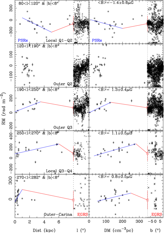
Figure 6: Same as Fig. 2 but for RMs for pulsars and EGRS in the outer Galactic zone. For this figure, the blue lines represent linear fits to the change in RM for most of the known pulsars in each zone. Postive slopes in the RM – DM plots indicate counter-clockwise fields for $l<180^{\circ}$ and clockwise fields for $l>180^{\circ}$.

3.3 Outer Galactic Zones for the local interarm region and the Perseus arm

It is well established that the Galactic magnetic field in the local region is clockwise (Manchester, 1974; Thomson & Nelson, 1980; Lyne & Smith, 1989; Han & Qiao, 1994; Rand & Lyne, 1994; Weisberg et al., 2004), implying a reversal between the local interarm region and the Carina – Sagittarius arm. This local clockwise field is confirmed by the decreasing RMs of pulsars with distance and DM in the subplot in Figure 6 for the region of $80^{\circ}<l<120^{\circ}$ and the increasing RMs in the subplots for the regions of $190^{\circ}<l<250^{\circ}$ and $250^{\circ}<l<270^{\circ}$, that is, Local Q1–Q2, Local Q3–Q4 and also Outer-Q3, where pulsars are nearer than or just within the Perseus arm (see Figure 1). We therefore conclude that the clockwise fields are dominant in the Carina – Perseus interarm zone, including the Local Arm region.

Comparison of RMs of pulsars and EGRS gives some evidence for counter-clockwise fields probably associated with the Perseus arm. First of all, as seen in Figure 6, in the region of $80^{\circ}<l<120^{\circ}$, pulsars show a systematic trend for RM decreasing. If there is no field reversal in the Perseus arm or outside, the RMs of EGRS are expected to be more negative. However, the data show that this is not the case. More positive RMs are observed for not only three distant pulsars ($D>6$ kpc) but also EGRS on average. A field reversal is also indicated by comparing the otherwise unexpected smaller RMs of EGRS in the outer regions of $190^{\circ}<l<250^{\circ}$ and $250^{\circ}<l<270^{\circ}$ with the increasing RMs of pulsars.

In the longitude region of $270^{\circ}<l<282^{\circ}$, random but predominantly positive RMs are observed for the local pulsars within 1 kpc, but RMs of EGRS are mostly negative which is probably an indication of counterclockwise fields in the Perseus arm implying a reversal from the local interarm field. If there were no field reversal and the Perseus-arm fields were clockwise, the RMs of distant pulsars and EGRS would be dominated by these clockwise fields and should be positive and increasing with distance. We do not have RMs of more distant pulsars, but the RMs of EGRS are consistent with reversed fields in the Perseus arm.

It is difficult to probe the large-scale structure of the magnetic field in the anti-center region of our Galaxy (e.g. in the region of $120^{\circ}<l<190^{\circ}$) using Faraday rotation since the uniform field tends to be perpendicular to the line of sight so that irregular field fluctuations can significantly influence the measured $B_{||}$. The RMs of pulsars in the Outer Q2 region are therefore more or less random.

Within the limitations imposed by uncertain distances, especially for the pulsar – EGRS regions, the field pattern illustrated in Figure 4 is consistent with our main conclusion, viz., that Galactic disk magnetic fields are predominantly counter-clockwise in spiral arms and clockwise in interarm regions, implying field reversals at each arm-interarm boundary. As is discussed further in the next section, this contrasts with the field patterns derived solely from EGRS RMs which generally have just one major region of clockwise field encompassing the whole Carina – Perseus region.

4 Modeling the Galactic disk magnetic field

Figure 4 shows the derived field directions listed in Table 1. In general according to the analysis above, counter-clockwise fields exist in the spiral arms and clockwise fields in the interarm regions. Comparison of extra-galactic RMs with distant pulsar RMs often indicate further reversals of field direction in the outer Galaxy. Because of the uncertain electron density, it is not possible to obtain quantitative estimates of $B_{||}$ in the regions beyond pulsars.

For the many applications where the strength and form of the Galactic magnetic field is important, it is useful to construct a simple model that can reflect the field reversals we discussed above for the Galactic disk and be used to estimate the large-scale field at a given Galactic location. Since we have only analysed the low-latitude RMs in this paper, our model just describes the structure of the Galactic disk field. A full three-dimensional model is left for future work.

Our model for the Galactic disk field assumes logarithmic spiral fields of pitch angle $\psi=11^{\circ}$ (Hou & Han, 2014) with a radial and $z$ dependence given by:

$$B(R,z)=B_{0}\exp(-R_{G}/A)\exp(-|z|/H)$$ (3)

where $R_{G}$ is the Galactocentric radial distance, $A$ is the disk radial scale and $H$ is the disk scale height. The field strength $B_{0}=B_{s}(i)$ for $R_{s}(i)<R_{0}<R_{s}(i+1)$, where $R_{s}(i)$ and $B_{s}(i)$ are given in Table 5 and $R_{0}$ is defined by

$$R_{0}=R_{G}\exp(-\psi\tan\theta)$$ (4)

where $\theta$ is the azimuth angle measured counterclockwise from the $+y$ axis, which points from the Galactic center to the Sun. For $R_{G}<R_{s}(1)$ and $R_{G}>$ 15 kpc, we set $B_{0}=0$.

Table 5: Radial zones for the model spiral disk field. Positive values of $B_{s}$ correspond to counter-clockwise fields and negative values to clockwise fields, as viewed from the north Galactic pole.

Index $i$	1	2	3	4	5	6	7
$R_{s}(i)$ (kpc)	3.0	4.1	4.9	6.1	7.5	8.5	10.5
$B_{s}(i)$ ($\mu$G)	4.5	$-3.0$	6.3	$-4.7$	3.3	$-8.7$	–

This field structure matches most of the field reversals we observe, and the values of $B_{s}(i)$ are generally consistent with the $\langle B\rangle$ values obtained from the gradients of the RM – DM fits in Figures 2 – 6, taking into account the location of the tangential point in Galactocentric radius and azimuth. The scale height of the disk field, $H$, was taken to be 0.4 kpc (cf., Jansson & Farrar, 2012) and the radial scale, $A$, was taken to be 5.0 kpc. The model field is illustrated in the left panel of Figure 7. The right panel of Figure 7 shows the Galactic disk field model of Jansson & Farrar (2012) (JF12) which is primarily based on RMs of EGRS.

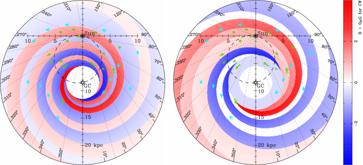
Figure 7: Left panel: Model for large-scale magnetic fields in the Galactic disk. Blue shading represents counter-clockwise fields and pink shading represents clockwise fields according to the bar on the right side of the figure. The arrows represent the inferred spiral field directions as shown in Figure 4. Right panel: The model of JF12 for large-scale magnetic fields in the Galactic disk based on RMs of EGRS and the Galactic synchrotron emission. The arrows are the same as in the left panel.

The new model, based on a combination of pulsar RMs and EGRS RMs, has between six and eight field reversals along a radial line from the Galactic Center, depending on the longitude. In contrast, the JF12 model of has clockwise disk fields across the whole Sagittarius – Carina region and no clockwise field in the Crux – Norma interarm region (tangential at $l=320^{\circ}$). As a consequence of this, there are only one or two reversals along radial lines from the Galactic Center. The clockwise field in the Crux – Norma tangential direction is clearly indicated by the positve pulsar RMs in this zone as shown in Figure 3. Similarly, the pulsar RMs shown in Figure 5 clearly show the presence of counter-clockwise fields in the Sagittarius tangential region as discussed above in §3.2.

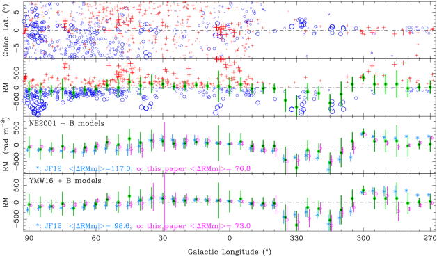
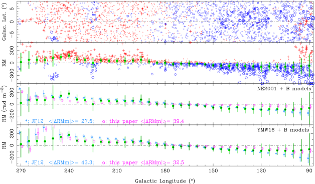
Figure 8: Distribution of RMs of EGRS with Galactic longitude, within $l=0^{\circ}\pm 90^{\circ}$ in the upper panel and $l=180^{\circ}\pm 90^{\circ}$ in the lower panel. For each panel, the top sub-panel shows the distribution of EGRS RMs in $b$, with blue circles representing RMs $<0$ and red + signs representing RMs $>0$, with the symbol size proportional to $|RM|^{1/2}$. The second sub-panel gives the RM magnitudes and their median values for every $5^{\circ}$ of Galactic longitude, with error bars representing the standard deviation from the median in the $5^{\circ}$ interval centered on the point. Where there were less than five RMs in the interval (primarily in Quadrant 4), the interval was extended (by steps of $2^{\circ}$) to encompass more than five points to give a realistic median and deviation. In the lower two sub-panels, the green points with error bars are as in the second panel, the pink circles and bars are the median values of the RMs computed for each source using the model for the disk field presented in this paper and the blue asterisks and bars are those computed using the JF12 model, for the NE2001 electron density model (Cordes & Lazio, 2002) and the YMW16 model (Yao et al., 2017), respectively. The model points and bars are slightly offset for clarity. Mean absolute differences between the median observed RMs and median predicted RMs weighted by the rms deviation of the observed RMs, $\langle|\Delta RM_{m}|\rangle$, is given for each field model and each electron density model in the lower sub-panels.

To compare how well these two models “predict” the EGRS RMs, we compute the RM of each EGRS source in Figure 1 using both the NE2001 electron density model (Cordes & Lazio, 2002), as used by JF12, and the more recent YMW16 model (Yao et al., 2017). In Figure 8 we show the distribution of observed EGRS RMs in Galactic latitude and longitude, along with the RMs computed using our model for the disk field, which is based on both pulsar and EGRS RMs, and from the JF12 model which is based on just the EGRS RMs. The RM median values for every $5^{\circ}$ of Galactic longitude are compared in the lower two sub-panels. This figure demonstrates that, despite its different structure and different basis, our model predicts RMs of EGRS more accurately than the JF12 model which is based primarily on them, for example, in the region $270^{\circ}\geq l\geq 280^{\circ}$. With the YMW16 electron density model (Yao et al., 2017), the weighted mean difference between the median observed RMs and median predicted RMs is smaller for our model in all quadrants. Even with the NE2001 model, our model is significantly better than predictions based on the JF12 model for the first and fourth quadrants (i.e., top panel of Figure 8).

However, the converse is not true. For example, as shown in the right panel of Figure 7, the EGRS-based model does not correctly model the clockwise fields in the Crux-Norma interarm region or the counter-clockwise fields in the Sagittarius-Carina arm. With their distribution through the Galactic disk at approximately known distances enabling tomographic mapping, pulsars are able to reveal reversals in the large-scale disk field that are concealed in the RMs of EGRS since they integrate across the entire disk. Despite the large number of EGRS RMs in the outer regions of our Galaxy (i.e. within $l=180^{\circ}\pm 90^{\circ}$), the field structure is not well constrained without comparison with the RMs of foreground pulsars. Even though the number of pulsar RMs is relatively small compared to that of EGRS RMs, the pulsar RMs are a very powerful tool in investigations of the large-scale Galactic magnetic field.

5 Conclusions

We have measured rotation measures for 477 pulsars of which 441 are either new or improved over previous measurements. By analyzing the distribution of pulsar RMs and comparing RMs for pulsars and extra-galactic radio sources (EGRS) lying within $8^{\circ}$ of the Galactic Plane, we show that the large-scale disk field in the inner Galaxy probably has a bisymmetric form with reversals between spiral arm and interarm regions. Compared to the analysis in Han et al. (2006), we have a larger sample of pulsar RMs and have combined pulsar and EGRS data to show the reversals in the Galactic disk large-scale field more clearly. Most of these reversals are not apparent in EGRS RM measurements since these average over the whole path inside our Galaxy. Furthermore, pulsar RM and DM data can give direct measurements of the mean magnetic field strength in selected regions of the Galaxy, for example, zones around tangential points.

Based on these results, we present a quantitative model for the large-scale magnetic field in the Galactic disk, which not only models the spiral magnetic field reversals between arm and interarm regions, but also can reproduce the RM distribution of EGRS better than a recent model based on EGRS data alone.

In the future, more pulsar RMs and improved pulsar distances will become available, allowing the large-scale structure of the Galactic magnetic fields to be better constrained. More RMs of EGRS, particularly in the longitude zone from $260^{\circ}$ to $350^{\circ}$ can help to determine the magnetic field structure beyond the pulsars. Observations of higher-latitude RMs for both pulsars and EGRS may in future allow construction of a complete three-dimensional model of the large-scale Galactic magnetic field, which is a proposed project for the SKA (see e.g., Han et al., 2015).

References

- Baars et al. (1977) Baars, J. W. M., Genzel, R., Pauliny-Toth, I. I. K., & Witzel, A. 1977, A&A, 61, 99
- Battaner & Florido (2007) Battaner, E., & Florido, E. 2007, Astronomische Nachrichten, 328, 92
- Beck (2015) Beck, R. 2015, A&A, 578, A93
- Beck et al. (1996) Beck, R., Brandenburg, A., Moss, D., Shukurov, A., & Sokoloff, D. 1996, ARA&A, 34, 155
- Beck et al. (2003) Beck, R., Shukurov, A., Sokoloff, D., & Wielebinski, R. 2003, A&A, 411, 99
- Bennett et al. (2013) Bennett, C. L., Larson, D., Weiland, J. L., et al. 2013, ApJS, 208, 20
- Beuermann et al. (1985) Beuermann, K., Kanbach, G., & Berkhuijsen, E. M. 1985, A&A, 153, 17
- Bilitza & Reinisch (2008) Bilitza, D., & Reinisch, B. W. 2008, Adv. Space Res., 42, 599
- Boulares & Cox (1990) Boulares, A., & Cox, D. P. 1990, ApJ, 365, 544
- Brown et al. (2007) Brown, J. C., Haverkorn, M., Gaensler, B. M., et al. 2007, ApJ, 663, 258
- Brown et al. (2003) Brown, J. C., Taylor, A. R., & Jackel, B. J. 2003, ApJS, 145, 213
- Clemens et al. (2012) Clemens, D. P., Pinnick, A. F., Pavel, M. D., & Taylor, B. W. 2012, ApJS, 200, 19
- Cordes & Lazio (2002) Cordes, J. M., & Lazio, T. J. W. 2002, ArXiv:astro-ph/0207156, arXiv:astro-ph/0207156
- Crutcher (1999) Crutcher, R. M. 1999, ApJ, 520, 706
- Demorest (2007) Demorest, P. B. 2007, PhD thesis, University of California, Berkeley
- Ferdman et al. (2004) Ferdman, R. D., Stairs, I. H., Backer, D. C., et al. 2004, AAS Abstracts, 205, 111.01
- Fermi (1949) Fermi, E. 1949, Phys. Rev., 75, 1169
- Force et al. (2015) Force, M. M., Demorest, P., & Rankin, J. M. 2015, MNRAS, 453, 4485
- Hamilton et al. (1985) Hamilton, P. A., Hall, P. J., & Costa, M. E. 1985, MNRAS, 214, 5P
- Hamilton & Lyne (1987) Hamilton, P. A., & Lyne, A. G. 1987, MNRAS, 224, 1073
- Hamilton et al. (1977) Hamilton, P. A., McCulloch, P. M., Manchester, R. N., Ables, J. G., & Komesaroff, M. M. 1977, Nature, 265, 224
- Han (2017) Han, J. L. 2017, Ann. Rev. Astr. Ap., 55, 111
- Han et al. (2009) Han, J. L., Demorest, P. B., van Straten, W., & Lyne, A. G. 2009, ApJS, 181, 557
- Han et al. (1997) Han, J. L., Manchester, R. N., Berkhuijsen, E. M., & Beck, R. 1997, A&A, 322, 98
- Han et al. (2006) Han, J. L., Manchester, R. N., Lyne, A. G., Qiao, G. J., & van Straten, W. 2006, ApJ, 642, 868
- Han et al. (1999) Han, J. L., Manchester, R. N., & Qiao, G. J. 1999, MNRAS, 306, 371
- Han & Qiao (1994) Han, J. L., & Qiao, G. J. 1994, A&A, 288, 759
- Han et al. (2015) Han, J. L., van Straten, W., Lazio, T. J. W., et al. 2015, Advancing Astrophysics with the Square Kilometre Array (AASKA14), 41
- Hankins & Rankin (2010) Hankins, T. H., & Rankin, J. M. 2010, AJ, 139, 168
- Heiles (1996) Heiles, C. 1996, ApJ, 462, 316
- Hotan et al. (2004) Hotan, A. W., van Straten, W., & Manchester, R. N. 2004, PASA, 21, 302
- Hou & Han (2014) Hou, L. G., & Han, J. L. 2014, A&A, 569, A125
- Indrani & Deshpande (1999) Indrani, C., & Deshpande, A. A. 1999, New Astr., 4, 33
- Jansson & Farrar (2012) Jansson, R., & Farrar, G. R. 2012, ApJ, 757, 14
- Johnston et al. (2005) Johnston, S., Hobbs, G., Vigeland, S., et al. 2005, MNRAS, 364, 1397
- Johnston et al. (2007) Johnston, S., Kramer, M., Karastergiou, A., et al. 2007, MNRAS, 381, 1625
- Kerr et al. (2014) Kerr, M., Hobbs, G., Shannon, R. M., et al. 2014, MNRAS, 445, 320
- Kiepenheuer (1950) Kiepenheuer, K. O. 1950, Physical Review, 79, 738
- Lyne & Smith (1989) Lyne, A. G., & Smith, F. G. 1989, MNRAS, 237, 533
- Manchester (1972) Manchester, R. N. 1972, ApJ, 172, 43
- Manchester (1974) Manchester, R. N. 1974, ApJ, 188, 637
- Manchester & Han (2004) Manchester, R. N., & Han, J. L. 2004, ApJ, 609, 354
- Manchester et al. (2005) Manchester, R. N., Hobbs, G. B., Teoh, A., & Hobbs, M. 2005, AJ, 129, 1993
- Manchester et al. (2013) Manchester, R. N., Hobbs, G., Bailes, M., et al. 2013, PASA, 30, 17
- Men et al. (2008) Men, H., Ferrière, K., & Han, J. L. 2008, A&A, 486, 819
- Navarro et al. (1997) Navarro, J., Manchester, R. N., Sandhu, J. S., Kulkarni, S. R., & Bailes, M. 1997, ApJ, 486, 1019
- Nota & Katgert (2010) Nota, T., & Katgert, P. 2010, A&A, 513, A65+
- Noutsos et al. (2008) Noutsos, A., Johnston, S., Kramer, M., & Karastergiou, A. 2008, MNRAS, 386, 1881
- Noutsos et al. (2015) Noutsos, A., Sobey, C., Kondratiev, V. I., et al. 2015, ArXiv e-prints, arXiv:ArXiv:1501.03312
- Novak et al. (2003) Novak, G., Chuss, D. T., Renbarger, T., et al. 2003, ApJ, 583, L83
- Ordog et al. (2017) Ordog, A., Brown, J. C., Kothes, R., & Landecker, T. L. 2017, ArXiv:1704.08663, arXiv:1704.08663
- Planck Collaboration et al. (2016a) Planck Collaboration, Adam, R., Ade, P. A. R., et al. 2016a, A&A, 594, A1
- Planck Collaboration et al. (2016b) Planck Collaboration, Ade, P. A. R., Aghanim, N., et al. 2016b, A&A, 586, A138
- Press et al. (1996) Press, W. H., Teukolsky, S. A., Vetterling, W. T., & Flannery, B. P. 1996, Numerical Recipes in Fortran 77: The Art of Scientific Computing, 2nd edition (Cambridge: Cambridge University Press)
- Pshirkov et al. (2011) Pshirkov, M. S., Tinyakov, P. G., Kronberg, P. P., & Newton-McGee, K. J. 2011, ApJ, 738, 192
- Qiao et al. (1995) Qiao, G. J., Manchester, R. N., Lyne, A. G., & Gould, D. M. 1995, MNRAS, 274, 572
- Ramachandran et al. (2004) Ramachandran, R., Backer, D. C., Rankin, J. M., Weisberg, J. M., & Devine, K. E. 2004, ApJ, 606, 1167
- Rand & Kulkarni (1989) Rand, R. J., & Kulkarni, S. R. 1989, ApJ, 343, 760
- Rand & Lyne (1994) Rand, R. J., & Lyne, A. G. 1994, MNRAS, 268, 497
- Rees (1987) Rees, M. J. 1987, QJRAS, 28, 197
- Simard-Normandin & Kronberg (1980) Simard-Normandin, M., & Kronberg, P. P. 1980, ApJ, 242, 74
- Sofue & Fujimoto (1983) Sofue, Y., & Fujimoto, M. 1983, apj, 265, 722
- Staveley-Smith et al. (1996) Staveley-Smith, L., Wilson, W. E., Bird, T. S., et al. 1996, PASA, 13, 243
- Sun & Reich (2010) Sun, X.-H., & Reich, W. 2010, Res. Astron. Astrophys., 10, 1287
- Sun et al. (2008) Sun, X. H., Reich, W., Waelkens, A., & Enßlin, T. A. 2008, A&A, 477, 573
- Taylor et al. (2009) Taylor, A. R., Stil, J. M., & Sunstrum, C. 2009, ApJ, 702, 1230
- Taylor et al. (1993) Taylor, J. H., Manchester, R. N., & Lyne, A. G. 1993, ApJS, 88, 529
- Thomson & Nelson (1980) Thomson, R. C., & Nelson, A. H. 1980, MNRAS, 191, 863
- Tiburzi et al. (2013) Tiburzi, C., Johnston, S., Bailes, M., et al. 2013, MNRAS, 436, 3557
- Vallée (1996) Vallée, J. P. 1996, A&A, 308, 433
- Vallée (2005) —. 2005, ApJ, 619, 297
- Van Eck et al. (2011) Van Eck, C. L., Brown, J. C., Stil, J. M., et al. 2011, ApJ, 728, 97
- van Ommen et al. (1997) van Ommen, T. D., D’Alesssandro, F. D., Hamilton, P. A., & McCulloch, P. M. 1997, MNRAS, 287, 307
- Vlemmings (2008) Vlemmings, W. H. T. 2008, A&A, 484, 773
- Weisberg et al. (2004) Weisberg, J. M., Cordes, J. M., Kuan, B., et al. 2004, ApJS, 150, 317
- Weltevrede & Johnston (2008) Weltevrede, P., & Johnston, S. 2008, MNRAS, 391, 1210
- Wu et al. (2015) Wu, Q., Kim, J., & Ryu, D. 2015, New Astron., 34, 21
- Wu et al. (2009) Wu, Q., Kim, J., Ryu, D., Cho, J., & Alexander, P. 2009, ApJ, 705, L86
- Xu & Han (2014) Xu, J., & Han, J.-L. 2014, Res. Astron. Astrophys., 14, 942
- Yan et al. (2011) Yan, W. M., Manchester, R. N., van Straten, W., et al. 2011, MNRAS, 414, 2087
- Yao et al. (2017) Yao, J. M., Manchester, R. N., & Wang, N. 2017, ApJ, 835, 29