A Scalable Deep Neural Network Architecture for Multi-Building and Multi-Floor Indoor Localization Based on Wi-Fi Fingerprinting

Abstract

One of the key technologies for future large-scale location-aware services covering a complex of multi-story buildings — e.g., a big shopping mall and a university campus — is a scalable indoor localization technique. In this paper, we report the current status of our investigation on the use of deep neural networks (DNNs) for scalable building/floor classification and floor-level position estimation based on Wi-Fi fingerprinting. Exploiting the hierarchical nature of the building/floor estimation and floor-level coordinates estimation of a location, we propose a new DNN architecture consisting of a stacked autoencoder for the reduction of feature space dimension and a feed-forward classifier for multi-label classification of building/floor/location, on which the multi-building and multi-floor indoor localization system based on Wi-Fi fingerprinting is built. Experimental results for the performance of building/floor estimation and floor-level coordinates estimation of a given location demonstrate the feasibility of the proposed DNN-based indoor localization system, which can provide near state-of-the-art performance using a single DNN, for the implementation with lower complexity and energy consumption at mobile devices.

Research

An earlier version of this paper was presented in part at ICUMT/FOAN 2017, Munich, Germany, November 2017.

1 Introduction

Location fingerprinting using received signal strengths (RSSs) from wireless network infrastructure is one of the most popular and promising technologies for localization in an indoor environment, where there is no line-of-sight signal from the global positioning system (GPS) available [1]: For example, a vector of pairs of a service set identifier (SSID) and an RSS for a Wi-Fi access point (AP) measured at a location can be its location fingerprint. A location of a user/device then can be estimated by finding the closest match between its RSS measurement and the fingerprints of known locations in a database [2]. Note that the location fingerprinting technique does not require the installation of any new infrastructure or the modification of existing devices, but it is just based on the existing wireless infrastructure, which is its major advantage over alternative techniques.

When the indoor localization is to cover a large building complex — e.g., a big shopping mall or a university campus — where there are lots of multi-story buildings under the same management, the scalability of fingerprinting techniques becomes an important issue. The current state-of-the-art Wi-Fi fingerprinting techniques assume a hierarchical approach to the indoor localization, where the building, floor, and position (e.g., a label or coordinates) of a location are estimated in a hierarchical and sequential way using a different algorithm tailored for each task. In [3], for instance, building estimation is done as follows: Given the AP with the strongest RSS in a measured fingerprint, we first build a subset of fingerprints where the same AP has the strongest RSS; then, we count the number of fingerprints associated to each building and set the estimated building to be the most frequent one from the counting. Similar procedures are also proposed to estimate a floor inside the building. For the estimation of the coordinates of the location, we first build a subset of fingerprints belonging to the building and the floor estimated from the previous procedures. Then, take multiple fingerprints from the subset most similar to the measured one, and compute the centroid of the coordinates of the selected fingerprints as the estimated coordinates of the given location. According to the results in [3], the best building and floor hit rates achieved for the UJIIndoorLoc dataset [4] are 100% and 94%, respectively, and the mean error in coordinates estimation is $6.20\text{\,}\mathrm{m}$.

One of the major challenges in Wi-Fi fingerprinting is how to deal with the random fluctuation of a signal, the noise from multi-path effects, and the device & position dependency in RSS measurements. Unlike traditional solutions relying on complex filtering and time-consuming parameter tuning specific to given conditions, the popular deep neural networks (DNNs) can provide attractive solutions to Wi-Fi fingerprinting due to their less parameter tuning and adaptability to a wider range of conditions with standard architectures and training algorithms [5, 6, 7]: In [5], a four-layer DNN generates a coarse positioning estimate, which, in turn, is refined to produce a final position estimate by a hidden Markov model (HMM)-based fine localizer. The performance of the proposed indoor localization system is evaluated in both indoor and outdoor environments which are divided into hundreds of square grids. In [6], the authors investigate the application of deep belief networks (DBNs) with two different types of Restricted Boltzmann Machines for indoor localization and evaluate the performance of their approaches using data from simulation in heterogeneous mobile radio networks using ray tracing techniques. In both cases, the authors focus only on the localization in a single plane and do not consider the hierarchical nature of multi-building and multi-floor indoor localization. In [7], on the other hand, a DNN consisting of a stacked autoencoder (SAE) and a feed-forward multi-class classifier is used for building/floor classification. This work, too, does not take into account the hierarchical nature of building/floor classification, because the classification is done over flattened, one-dimensional labels of combined building and floor identifiers. Also, the floor-level location estimation is not considered at all. In this regard, to the best of our knowledge, the work presented in this paper is the first to apply DNNs for multi-building and multi-floor indoor localization, exploiting its hierarchical nature in classification.

In this paper, we report the current status of our investigation on the use of DNNs for scalable building/floor classification and floor-level location estimation. We propose a new DNN architecture consisting of an SAE for the reduction of feature space dimension and a feed-forward multi-label classifier [8, 9] for a multi-building and multi-floor indoor localization system based on Wi-Fi fingerprinting and evaluate its performance using the UJIIndoorLoc dataset [4].

The rest of the paper is organized as follows: In Sec. 2, we describe the problem of indoor localization in a large building complex with its challenges resulting from the existence of multi-story buildings and propose a scalable DNN architecture for the multi-building and multi-floor indoor localization. Sec. 3 provides and discusses experimental results for the performance of the proposed scalable DNN-based multi-building and multi-floor indoor localization system. Sec. 4 concludes our work in this paper and suggests areas of further research.

2 A Scalable DNN Architecture for Multi-Building and Multi-Floor Indoor Localization

Location awareness is one of enabling technologies for future smart and green cities; understanding where people spend their times and how they interact with environments is critical to realizing the vision of smart and green cities [10]. One of the key technologies for future large-scale location-aware services covering a complex of multi-story buildings — e.g., a big shopping mall and a university campus — is a scalable indoor localization technique. Regarding the scalability of the indoor localization, consider the evolution of the Xi’an Jiaotong-Liverpool University (XJTLU) campus in Suzhou, China, where the authors are currently working: As shown in Figure 1 (a), the XJTLU started with just one building in 2006. As of this writing, the XJTLU has two campuses, which are shown in Figure 1 (b), and the number of buildings over two campuses has increased to around 20; this number is still increasing as more buildings and sports facilities are being constructed. Considering all the floors within each building and the locations on each floor, the total number of distinct locations (e.g., offices, lecture rooms, and labs) is already on the order of thousands. If we adopt a grid-based representation of the localization area as in [5], the total number of locations would be even greater. The indoor localization system to cover such a large building complex, therefore, must be scalable.

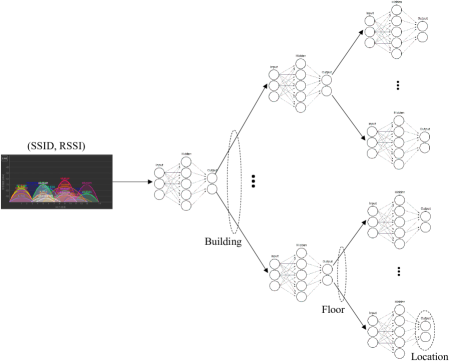
(a)

(b)

Figure 2: System architectures for large-scale DNN-based multi-building and multi-floor indoor localization: (a) A hierarchical architecture; (b) an integrated architecture.

Figure 2 shows two alternative system architectures for large-scale DNN-based multi-building and multi-floor indoor localization. In the hierarchical architecture shown in Figure 2 (a), the task of building/floor/location classification is separated into multiple sub-tasks dedicated to the classification at each level of building, floor, and location. This architecture directly corresponds to the state-of-the-art hierarchical Wi-Fi fingerprinting methods (e.g., [3]), where DNNs replace traditional techniques for building, floor, and location estimation. Compared to the methods based on traditional techniques, a major disadvantage in this hierarchical DNN architecture is that the DNNs in the floor and the location levels of the system need to be trained separately with multiple sub-datasets derived from a common dataset (i.e., building-specific datasets for DNNs for floor estimation and building-floor-specific datasets for DNNs for location estimation), which poses significant challenges on the management of location fingerprint databases as well as the training of possibly a large number of DNNs. In this paper, therefore, we focus on the integrated architecture shown in Figure 2 (b) where a single DNN handles the classification of building, floor, and location in an integrated way with a common dataset.

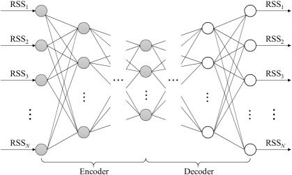
(a)

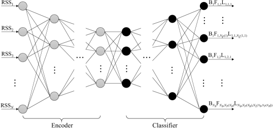
(b)

Figure 3: A DNN architectures for the combined estimation of building, floor, and location: (a) A stacked autoencoder (SAE) for the reduction of feature space dimension; (b) an overall architecture consisting of the encoder part of the SAE and a feed-forward classifier for multi-class classification with flattened building-floor-location labels as in [7].

Figure 3 shows a DNN architecture for the combined estimation of building, floor, and location based on multi-class classification with flattened labels, which is a straightforward extension of the DNN system for building/floor classification proposed in [7]; after training with RSSs as both input and output data as shown in Figure 3 (a), only the gray-colored nodes are used as an encoder for feature space dimension reduction as shown in Figure 3 (b). This DNN architecture based on multi-class classification with flattened labels, however, has the scalability issue that the number of output nodes is equal to the number of locations over the building complex: In case of the UJIIndoorLoc dataset, the number of distinct locations (i.e., also called reference points in [4]) over 3 buildings with 4 or 5 floors is 933. It also does not take into account the hierarchical nature of the building/floor/location classification problem due to its calculating the loss and the accuracy over flattened building/floor/location labels; the misclassification of building, floor, or location has equal loss during the training phase. To reflect the hierarchical nature of the building/floor/location classification in a DNN classifier, one can use a hierarchical loss function — e.g., a loss function with different weights for building, floor, and location — with the existing multi-class classifier and flattened labels. Because the hierarchical loss function for flattened labels is quite complicated and does not provide a closed-form gradient function, however, training the DNN with the usual backpropagation procedure could be challenging.

To address the scalability issue of the DNN classifier based on multi-class classification and take into account the hierarchical nature of the building/floor/location classification, we propose a scalable DNN architecture based on multi-label classification shown in Figure 4. The building/floor/location classification with the proposed architecture is done as follows: First, building, floor, and location identifiers are mapped to sequential numbers, the latter two of which are meaningful only in combination with higher-level numbers; those numbers are one-hot encoded independently and combined together into a vector as a categorical variable for multi-label classification as illustrated in Table. 1. Then, the output vector from the multi-label classifier is split into a building, a floor, and a location vector by indexes as shown in Figure 4. Finally, we estimate the building and the floor of a location as the index of a maximum value of the corresponding vector through the $\operatorname*{arg\,max}$ function. For the estimation of the location coordinates, we select $\kappa$ largest elements from the location vector (i.e., $\boldsymbol{L}{=}\big{(}\text{L}_{1},\ldots,\text{L}_{\max(\ldots,N_{L}(i.j))}\big{)}$ in Figure 4), filter out the elements whose values are less than $\sigma{\times}\max(\boldsymbol{L})$ ($\sigma{\in}[0,1]$), and calculate the estimated coordinates of the location as either the normal or weighted (with the values of the elements as weights) centroid of the remaining elements as described in detail in Figure 1.

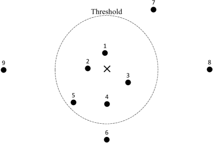
(a)

(b)

Figure 5: Two examples of location coordinates estimation, where $\boldsymbol{\times}$ denotes a new location whose coordinates are to be estimated and $\CIRCLE$ denotes a reference point whose coordinates are stored in the fingerprint database. The numbers over the reference points indicate their closeness to the new location with 1 being the closest.

Note that there are two design parameters — i.e., $\kappa$ and $\sigma$ — in the location coordinates estimation procedure, the rationale of which is illustrated in Figure 5: If we use only $\kappa$ as a design parameter as in [3] and sets its value to 5 in Figure 5 (a), we can include the reference points quite close to the new location (i.e., those inside the dotted circle) in the estimation procedure and can generate good estimation. In Figure 5 (b), however, the same value of $\kappa$ could result in poor estimation because the reference points 4 and 5 have to be considered during the estimation. With $\kappa{=}3$, on the other hand, we can expect good estimation with Figure 5 (b) but not with Figure 5 (a) this time. If we can use both $\kappa$ and $\sigma$ as design parameters, however, we can include good reference points by properly setting $\sigma$ for a threshold value. The actual effects of these design parameters on the location coordinates estimation are investigated in Sec. 3.

As for the scalability of the proposed DNN architecture, the number of output nodes becomes much smaller than that of the DNN architecture based on multi-class classification: The number of output nodes for multi-label building/floor/location classification is given by

$$N_{B} +\max\Big{(}N_{F}(1),\ldots,N_{F}(N_{B})\Big{)}$$ (1)

$$+\max\Big{(}N_{L}(1,1),\ldots,N_{L}\big{(}N_{B},N_{F}(N_{B})\big{)}\Big{)},$$

where $N_{B}$, $N_{F}(i)$, and $N_{L}(j,k)$ are the number of buildings in the complex, the number of floors in the $i$th building ($i=1,\ldots,N_{B}$), and the number of locations on the $k$th floor of the $j$th building ($j=1,\ldots,N_{B}$; $k=1,\ldots,N_{F}(j)$), respectively. Note that for multi-class building/floor/location classification, the number becomes

$$\sum_{i=1}^{N_{B}}\sum_{j=1}^{N_{F}(i)}N_{L}(i,j).$$ (2)

According to (1), the number of output nodes of the proposed DNN architecture for the publicly available UJIIndoorLoc dataset at the University of California, Irvine (UCI), Machine Learning Repository is given by 118 (i.e., the sum of the number of buildings (3), the maximum of the numbers of floors of the buildings (5), and the maximum of the numbers of locations on the floors (110)), which is smaller than the number of output nodes of the DNN architecture based on multi-class classification (i.e., 905). Note that the difference could be much larger if the UJIIndoorLoc dataset covers all the buildings on the Jaume I University (UJI) campus where the data were collected.

Also, due to the clear mapping between building, floor, and location identifiers and its corresponding one-hot-encoded categorical variable for the DNN-based multi-label classifier, it is easy to carry out different processing for parts of DNN outputs specifically for building, floor, and location as illustrated in Figure 4. Especially, the use of multiple elements in estimating location coordinates is a huge advantage in terms of computational complexity because trained DNNs can generate multi-dimensional output values in parallel; in traditional approaches, on the other hand, selecting nearest locations based on Euclidean distances are complex and time consuming. This flexibility in handling DNN outputs also makes it easy to apply different weights to the cost of building, floor, and location classification error during the training phase.

3 Experimental Results

We carried out experiments using the UJIIndoorLoc dataset [4] to evaluate the performance of the proposed DNN-based multi-building and multi-floor indoor localization system. We focus on the effects of the number of largest elements from the output location vector (i.e., $\kappa$) and the scaling factor for a threshold (i.e., $\sigma$) in the location coordinates estimation procedure described in Sec. 2. Table 2 summarizes DNN parameter values for the experiments, which are chosen experimentally and used throughout the experiments.

As indicated in [7], the publicly available UJIIndoorLoc dataset includes training and validation data, but not testing data which were provided only to the competitors at the Evaluating Ambient Assisted Living (EvAAL) competition at the International Conference on Indoor Positioning and Indoor Navigation (IPIN) 2015 [3]. Also, unlike the training data, the validation data do not include location information (i.e., SpaceID and RELATIVEPOSITION fields) because the measurements were taken at arbitrary points as would happen in a real localization system. In this regard, we split the training data into new training and validation data with the ratio of 70:30 for DNN training and validation with building/floor/location labels for both. During the evaluation phase, the output from the trained DNN are post-processed as described in Sec. 2 and compared with the building, floor, and coordinates of a given location. In this way, we can compare out results of multi-building and multi-floor indoor localization with the baseline and the best results from [4] and [3].

Table 3 summarizes our experimental results, which show the effects of the number of largest elements from the output location vector ($\kappa$) and the scaling factor for a threshold ($\sigma$) on the performance of multi-building and multi-floor indoor localization. We highlight in light gray the rows with success rate (i.e., the rate of successful estimation of both building and floor) higher than 90 % and positioning errors (both normal and weighted centroid) lower than $10\text{\,}\mathrm{m}$, respectively.

In general, $\sigma$ in the range of $0.10.3$ produces the best localization performance for $\kappa{\leq}8$; once $\kappa$ becomes larger than 8, however, higher values of $\sigma$ (i.e., 0.4 for $\kappa{=}9$ and 0.5 for $\kappa{=}10$) generate better performance. Considering the coordinates location estimation examples shown in Figure 5 with their explanations in Sec. 2 regarding the use of two design parameters, we can explain these results as follows: With a larger value of $\kappa$ (i.e., 9 and 10), there could be a higher chance of including reference points relatively far from the given location as shown in Figure 5 (b). In such a case, a tighter threshold (i.e., a larger value of $\sigma$) can filter out those reference points.

According to the results shown in Table 3, collectively the best results are achieved when $\kappa{=}8$ and $\sigma{=}0.2$, which are highlighted in gray. These results from the proposed DNN-based multi-building and multi-floor indoor localization system — i.e., 99.82 % for building hit rate, 91.27 % for floor hit rate, 91.18 % for success rate and $9.29\text{\,}\mathrm{m}$ for positioning error — are favorably comparable to the baseline results — i.e., 89.92 % for success rate and $7.9\text{\,}\mathrm{m}$ for positioning error — from [4] which are based on the distance-based $k$-Nearest Neighbors ($k$NN) algorithm [13]. As discussed in Sec. 2, even though a direct comparison with the results from the EvAAL/IPIN 2015 competition is not possible due to the lack of testing samples in the public version of the UJIIndoorLoc dataset and a slightly different way of calculating the positioning error, our results are also comparable to the competition results summarized in Table 4.

Note that the results presented in this section are not optimized with DNN parameters, including the number of hidden layers and the number of nodes at each layer; we investigated the feasibility of the combined building/floor/location estimation using a single DNN based on multi-label classification framework with focus on the effects of the number of largest elements from the output location vector ($\kappa$) and the scaling factor for a threshold ($\sigma$) in the location coordinates estimation. This leaves much room for further optimization of the performance.

4 Conclusions

In this paper we have proposed a new scalable DNN architecture for multi-building and multi-floor indoor localization based on Wi-Fi fingerprinting, which can cover a large-scale complex of many multi-story buildings under the same management. The proposed DNN architecture consists of an SAE for the reduction of feature space dimension and a feed-forward classifier for multi-label classification of building/floor/location. Reformulating the problem of building/floor/location classification based on the framework of multi-label classification, we can achieve better scalability (i.e., greatly reducing the number of DNN output nodes) and better exploit the hierarchical nature of the building/floor estimation and the floor-level location coordinates estimation through systematic label formation (i.e., providing straightforward mapping between a DNN categorical variable and building, floor & location vectors) compared to existing DNN architectures based on multi-class classification.

The experimental results using the UJIIndoorLoc dataset clearly demonstrate the feasibility of the proposed DNN-based multi-building and multi-floor indoor localization system, which can provide near state-of-the-art performance using a single DNN in an integrated way. Combined with the unique advantage of a DNN-based indoor localization system that, once trained, it does not need the fingerprint database any longer but carries the necessary information for localization in DNN weights, the scalable DNN architecture proposed in this paper could open a door for a future secure and energy-efficient indoor localization solution exclusively running on mobile devices without exchanging any data with the server.

Still, there are several areas for further research in multi-building and multi-floor indoor localization based on DNNs and Wi-Fi fingerprinting. First, the experimental results described in Sec. 3 are preliminary and not based on optimized DNN parameters; there are still much room for further optimization of the performance through DNN parameter tuning and the investigation of the performance and complexity tradeoff. Second, there is no direct match between the cost function used in DNN training/validation and the actual performance in the final evaluation for building/floor detection and the location coordinates estimation due to the additional processing of DNN output (i.e., the use of $\operatorname*{arg\,max}$ function for the former and the rather complicated processing with multiple elements of the location vector for the latter). To fully take into account the actual performance of building/floor detection and location coordinates estimation during training/validation, we may consider heuristics like evolutionary algorithms (e.g., genetic algorithm (GA) [14] and particle swarm optimization (PSO) [15]), simulated annealing [16], and quantum annealing [17] for training DNN weights; due to its many tradeoffs between complexity and flexibility resulting from the use of heuristics in DNN weight training, this approach could be an interesting topic for long-term research.

Competing interests

The authors declare that they have no competing interests.

Author’s contributions

Kyeong Soo Kim, Sanghyuk Lee, and Kaizhu Huang initiated a seed project on the subject of scalable indoor localization based on DNNs and Wi-Fi fingerprinting, which this manuscript is based on. Kyeong Soo Kim proposed DNN architectures, carried out numerical experiments, and drafted the manuscript, which Sanghyuk Lee and Kaizhu Huang checked and clarified. All authors read and approved the final manuscript.

Figures

(a)

(b)

Figure 1: XJTLU campus in (a) 2006 and (b) 2017.

Figure 4: A DNN architectures for scalable building/floor classification and floor-level coordinates estimation based on an SAE for the reduction of feature space dimension and a feed-forward classifier for multi-label classification.

Input : Training/validation dataset $\boldsymbol{\mathcal{D}}$

Input : Estimated building ID B_i

Input : Estimated floor ID F_j

Input : $\boldsymbol{\mathcal{L}}=\left\{\mathcal{L}_{1}\ldots\mathcal{L}_{\kappa}\right\}$, a set of $\kappa$ largest elements of the location vector $\boldsymbol{L}$ from the DNN classifier

Output : Estimated location coordinates $\boldsymbol{C_{s}}=(x_{s},y_{s})$ (centroid)

Output : Estimated location coordinates $\boldsymbol{C_{w}}=(x_{w},y_{w})$ (weighted centroid)

$sum_{x}\leftarrow 0$

$wsum_{x}\leftarrow 0$

$sum_{y}\leftarrow 0$

$wsum_{y}\leftarrow 0$

$sum_{w}\leftarrow 0$

$n_{c}\leftarrow 0$ // number of candidate coordinates

for $l\in\boldsymbol{\mathcal{L}}$ do

     if $l\geq\sigma{\times}\max(\boldsymbol{L})$ then // threshold checking

          if $(\text{B}_{i},\text{F}_{j},l)\in\boldsymbol{\mathcal{D}}$ then // i.e., a valid location of the dataset

               $x\leftarrow\operatorname*{coords}_{x}(\text{B}_{i},\text{F}_{j},l)$ // return the $x$ coordinate of building/floor/location

                $y\leftarrow\operatorname*{coords}_{y}(\text{B}_{i},\text{F}_{j},l)$ // return the $y$ coordinate of building/floor/location

                $sum_{x}\leftarrow sum_{x}+x$

                $wsum_{x}\leftarrow wsum_{x}+l{\times}x$

                $sum_{y}\leftarrow sum_{y}+y$

                $wsum_{y}\leftarrow wsum_{y}+l{\times}y$

                $sum_{w}\leftarrow sum_{w}+l$

                $n_{c}\leftarrow n_{c}+1$

                end if

               

                end if

               

                end for

               if $n_{c}>0$ then

                    $\boldsymbol{C_{s}}\leftarrow(\frac{sum_{x}}{n_{c}},\frac{sum_{y}}{n_{c}})$

                     $\boldsymbol{C_{w}}\leftarrow(\frac{wsum_{x}}{sum_{w}},\frac{wsum_{y}}{sum_{w}})$

                     end if

                    else // i.e., no candidate coordinates

                         $\boldsymbol{C_{s}},\boldsymbol{C_{w}}\leftarrow\text{centroid of {all} coordinates belonging to B${}_{i}$ and F${}_{j}$ of $\boldsymbol{\mathcal{D}}$}$

                          end if

Algorithm 1 Procedure for the estimation of location coordinates.

Tables

Table 1: Label formation example for the multi-label classification of building, floor, and location with two multi-story buildings.

Building	Floor	Location	Sequential Coding	One-Hot Coding
A	1st	Lecture Theater A	$0,0,0$	$01|0001|0001$
		Lecture Theater B	$0,0,1$	$01|0001|0010$
	2nd	Lab 1	$0,1,0$	$01|0010|0001$
		Lab 2	$0,1,1$	$01|0010|0010$
	3rd	A301	$0,2,0$	$01|0100|0001$
		A302	$0,2,1$	$01|0100|0010$
		A303	$0,2,2$	$01|0100|0100$
B	1st	Common Room	$1,0,0$	$10|0001|0001$
		Printing Room	$1,0,1$	$10|0001|0010$
	2nd	Conference Room 1	$1,1,0$	$10|0010|0001$
		Conference Room 2	$1,1,1$	$10|0010|0010$
	3rd	B301	$1,2,0$	$10|0100|0001$
		B302	$1,2,1$	$10|0100|0010$
		B303	$1,2,2$	$10|0100|0100$
		B304	$1,2,3$	$10|0100|1000$
	4th	Gym	$1,3,0$	$10|1000|0001$

Table 2: Parameter Values for Scalable DNN-Based Indoor Localization.

DNN Parameter	Value
Ratio of Training Data to Overall Data	0.90
Number of Epochs	20
Batch Size	10
SAE Hidden Layers	256-128-256
SAE Activation	Rectified Linear (ReLU)
SAE Optimizer	ADAM [18]
SAE Loss	Mean Squared Error (MSE)
Classifier Hidden Layers	64-128
Classifier Activation	ReLU
Classifier Optimizer	ADAM
Classifier Loss	Binary Crossentropy
Classifier Dropout Rate	0.20

Table 3: Effects of the number of largest elements from the output location vector ($\kappa$) and the scaling factor for a threshold ($\sigma$) on the Performance of multi-building and multi-floor indoor localization.

$\kappa$	$\sigma$	Building Hit Rate [%]	Floor Hit Rate [%]	Success Rate [%]	Positioning Error [m]
					Centroid	Weighted Centroid
1	N/A*	$9.981\,998\text{\times}{10}^{01}$	$9.189\,919\text{\times}{10}^{01}$	$9.180\,918\text{\times}{10}^{01}$	$1.140\,346\text{\times}{10}^{01}$	$1.140\,346\text{\times}{10}^{01}$
2	0.0	$9.936\,994\text{\times}{10}^{01}$	$9.243\,924\text{\times}{10}^{01}$	$9.180\,918\text{\times}{10}^{01}$	$1.062\,041\text{\times}{10}^{01}$	$1.053\,982\text{\times}{10}^{01}$
	0.1	$1.000\,000\text{\times}{10}^{02}$	$9.180\,918\text{\times}{10}^{01}$	$9.180\,918\text{\times}{10}^{01}$	$1.040\,084\text{\times}{10}^{01}$	$1.032\,711\text{\times}{10}^{01}$
	0.2	$9.981\,998\text{\times}{10}^{01}$	$9.261\,926\text{\times}{10}^{01}$	$9.243\,924\text{\times}{10}^{01}$	$9.739\,654\text{\times}{10}^{00}$	$9.661\,333\text{\times}{10}^{00}$
	0.3	$9.963\,996\text{\times}{10}^{01}$	$9.198\,920\text{\times}{10}^{01}$	$9.180\,918\text{\times}{10}^{01}$	$9.777\,987\text{\times}{10}^{00}$	$9.710\,835\text{\times}{10}^{00}$
	0.4	$9.972\,997\text{\times}{10}^{01}$	$9.153\,915\text{\times}{10}^{01}$	$9.144\,914\text{\times}{10}^{01}$	$1.028\,777\text{\times}{10}^{01}$	$1.020\,546\text{\times}{10}^{01}$
	0.5	$1.000\,000\text{\times}{10}^{02}$	$9.000\,900\text{\times}{10}^{01}$	$9.000\,900\text{\times}{10}^{01}$	$1.015\,949\text{\times}{10}^{01}$	$1.009\,243\text{\times}{10}^{01}$
3	0.0	$9.972\,997\text{\times}{10}^{01}$	$9.153\,915\text{\times}{10}^{01}$	$9.135\,914\text{\times}{10}^{01}$	$1.014\,222\text{\times}{10}^{01}$	$9.792\,770\text{\times}{10}^{00}$
	0.1	$9.990\,999\text{\times}{10}^{01}$	$9.090\,909\text{\times}{10}^{01}$	$9.081\,908\text{\times}{10}^{01}$	$9.918\,299\text{\times}{10}^{00}$	$9.758\,788\text{\times}{10}^{00}$
	0.2	$9.882\,988\text{\times}{10}^{01}$	$9.090\,909\text{\times}{10}^{01}$	$9.027\,903\text{\times}{10}^{01}$	$9.983\,135\text{\times}{10}^{00}$	$9.795\,777\text{\times}{10}^{00}$
	0.3	$9.954\,995\text{\times}{10}^{01}$	$9.207\,921\text{\times}{10}^{01}$	$9.189\,919\text{\times}{10}^{01}$	$1.013\,391\text{\times}{10}^{01}$	$1.000\,786\text{\times}{10}^{01}$
	0.4	$9.990\,999\text{\times}{10}^{01}$	$9.198\,920\text{\times}{10}^{01}$	$9.198\,920\text{\times}{10}^{01}$	$1.063\,061\text{\times}{10}^{01}$	$1.047\,131\text{\times}{10}^{01}$
	0.5	$9.981\,998\text{\times}{10}^{01}$	$9.036\,904\text{\times}{10}^{01}$	$9.036\,904\text{\times}{10}^{01}$	$9.937\,904\text{\times}{10}^{00}$	$9.889\,872\text{\times}{10}^{00}$
4	0.0	$9.981\,998\text{\times}{10}^{01}$	$9.090\,909\text{\times}{10}^{01}$	$9.090\,909\text{\times}{10}^{01}$	$1.027\,489\text{\times}{10}^{01}$	$9.662\,943\text{\times}{10}^{00}$
	0.1	$9.936\,994\text{\times}{10}^{01}$	$9.198\,920\text{\times}{10}^{01}$	$9.162\,916\text{\times}{10}^{01}$	$1.036\,905\text{\times}{10}^{01}$	$9.920\,916\text{\times}{10}^{00}$
	0.2	$9.963\,996\text{\times}{10}^{01}$	$9.207\,921\text{\times}{10}^{01}$	$9.189\,919\text{\times}{10}^{01}$	$1.025\,626\text{\times}{10}^{01}$	$1.008\,654\text{\times}{10}^{01}$
	0.3	$9.981\,998\text{\times}{10}^{01}$	$9.144\,914\text{\times}{10}^{01}$	$9.135\,914\text{\times}{10}^{01}$	$1.023\,558\text{\times}{10}^{01}$	$1.015\,537\text{\times}{10}^{01}$
	0.4	$9.990\,999\text{\times}{10}^{01}$	$9.225\,923\text{\times}{10}^{01}$	$9.216\,922\text{\times}{10}^{01}$	$1.034\,791\text{\times}{10}^{01}$	$1.023\,167\text{\times}{10}^{01}$
	0.5	$9.981\,998\text{\times}{10}^{01}$	$9.126\,913\text{\times}{10}^{01}$	$9.117\,912\text{\times}{10}^{01}$	$1.009\,757\text{\times}{10}^{01}$	$1.007\,306\text{\times}{10}^{01}$
5	0.0	$9.990\,999\text{\times}{10}^{01}$	$9.135\,914\text{\times}{10}^{01}$	$9.126\,913\text{\times}{10}^{01}$	$1.128\,615\text{\times}{10}^{01}$	$1.036\,350\text{\times}{10}^{01}$
	0.1	$9.990\,999\text{\times}{10}^{01}$	$9.162\,916\text{\times}{10}^{01}$	$9.162\,916\text{\times}{10}^{01}$	$9.897\,813\text{\times}{10}^{00}$	$9.618\,697\text{\times}{10}^{00}$
	0.2	$9.990\,999\text{\times}{10}^{01}$	$9.072\,907\text{\times}{10}^{01}$	$9.072\,907\text{\times}{10}^{01}$	$9.887\,615\text{\times}{10}^{00}$	$9.571\,252\text{\times}{10}^{00}$
	0.3	$9.981\,998\text{\times}{10}^{01}$	$9.090\,909\text{\times}{10}^{01}$	$9.081\,908\text{\times}{10}^{01}$	$1.026\,534\text{\times}{10}^{01}$	$9.992\,006\text{\times}{10}^{00}$
	0.4	$9.972\,997\text{\times}{10}^{01}$	$9.216\,922\text{\times}{10}^{01}$	$9.207\,921\text{\times}{10}^{01}$	$1.016\,706\text{\times}{10}^{01}$	$1.001\,166\text{\times}{10}^{01}$
	0.5	$9.981\,998\text{\times}{10}^{01}$	$9.297\,930\text{\times}{10}^{01}$	$9.288\,929\text{\times}{10}^{01}$	$1.059\,074\text{\times}{10}^{01}$	$1.053\,813\text{\times}{10}^{01}$
6	0.0	$9.981\,998\text{\times}{10}^{01}$	$9.189\,919\text{\times}{10}^{01}$	$9.171\,917\text{\times}{10}^{01}$	$1.084\,073\text{\times}{10}^{01}$	$9.713\,978\text{\times}{10}^{00}$
	0.1	$9.963\,996\text{\times}{10}^{01}$	$9.207\,921\text{\times}{10}^{01}$	$9.180\,918\text{\times}{10}^{01}$	$1.035\,306\text{\times}{10}^{01}$	$9.861\,424\text{\times}{10}^{00}$
	0.2	$1.000\,000\text{\times}{10}^{02}$	$9.198\,920\text{\times}{10}^{01}$	$9.198\,920\text{\times}{10}^{01}$	$9.853\,155\text{\times}{10}^{00}$	$9.564\,450\text{\times}{10}^{00}$
	0.3	$9.981\,998\text{\times}{10}^{01}$	$9.279\,928\text{\times}{10}^{01}$	$9.279\,928\text{\times}{10}^{01}$	$1.048\,978\text{\times}{10}^{01}$	$1.022\,295\text{\times}{10}^{01}$
	0.4	$9.936\,994\text{\times}{10}^{01}$	$9.108\,911\text{\times}{10}^{01}$	$9.099\,910\text{\times}{10}^{01}$	$1.032\,216\text{\times}{10}^{01}$	$1.017\,355\text{\times}{10}^{01}$
	0.5	$9.963\,996\text{\times}{10}^{01}$	$9.090\,909\text{\times}{10}^{01}$	$9.063\,906\text{\times}{10}^{01}$	$9.554\,220\text{\times}{10}^{00}$	$9.519\,261\text{\times}{10}^{00}$
7	0.0	$9.981\,998\text{\times}{10}^{01}$	$8.928\,893\text{\times}{10}^{01}$	$8.928\,893\text{\times}{10}^{01}$	$1.174\,417\text{\times}{10}^{01}$	$1.022\,120\text{\times}{10}^{01}$
	0.1	$9.981\,998\text{\times}{10}^{01}$	$9.018\,902\text{\times}{10}^{01}$	$9.000\,900\text{\times}{10}^{01}$	$1.042\,525\text{\times}{10}^{01}$	$9.820\,845\text{\times}{10}^{00}$
	0.2	$9.990\,999\text{\times}{10}^{01}$	$9.144\,914\text{\times}{10}^{01}$	$9.144\,914\text{\times}{10}^{01}$	$1.000\,036\text{\times}{10}^{01}$	$9.551\,645\text{\times}{10}^{00}$
	0.3	$9.990\,999\text{\times}{10}^{01}$	$9.162\,916\text{\times}{10}^{01}$	$9.153\,915\text{\times}{10}^{01}$	$9.746\,898\text{\times}{10}^{00}$	$9.533\,490\text{\times}{10}^{00}$
	0.4	$9.963\,996\text{\times}{10}^{01}$	$9.045\,905\text{\times}{10}^{01}$	$9.018\,902\text{\times}{10}^{01}$	$1.041\,638\text{\times}{10}^{01}$	$1.028\,135\text{\times}{10}^{01}$
	0.5	$9.954\,995\text{\times}{10}^{01}$	$9.144\,914\text{\times}{10}^{01}$	$9.135\,914\text{\times}{10}^{01}$	$9.830\,048\text{\times}{10}^{00}$	$9.733\,772\text{\times}{10}^{00}$
8	0.0	$9.990\,999\text{\times}{10}^{01}$	$9.018\,902\text{\times}{10}^{01}$	$9.009\,901\text{\times}{10}^{01}$	$1.131\,833\text{\times}{10}^{01}$	$9.270\,887\text{\times}{10}^{00}$
	0.1	$1.000\,000\text{\times}{10}^{02}$	$9.126\,913\text{\times}{10}^{01}$	$9.126\,913\text{\times}{10}^{01}$	$1.061\,573\text{\times}{10}^{01}$	$1.014\,184\text{\times}{10}^{01}$
	0.2	$9.981\,998\text{\times}{10}^{01}$	$9.126\,913\text{\times}{10}^{01}$	$9.117\,912\text{\times}{10}^{01}$	$9.755\,503\text{\times}{10}^{00}$	$9.285\,992\text{\times}{10}^{00}$
	0.3	$9.981\,998\text{\times}{10}^{01}$	$9.054\,905\text{\times}{10}^{01}$	$9.036\,904\text{\times}{10}^{01}$	$9.953\,853\text{\times}{10}^{00}$	$9.819\,975\text{\times}{10}^{00}$
	0.4	$9.990\,999\text{\times}{10}^{01}$	$9.036\,904\text{\times}{10}^{01}$	$9.027\,903\text{\times}{10}^{01}$	$1.021\,126\text{\times}{10}^{01}$	$1.013\,918\text{\times}{10}^{01}$
	0.5	$9.990\,999\text{\times}{10}^{01}$	$9.054\,905\text{\times}{10}^{01}$	$9.054\,905\text{\times}{10}^{01}$	$9.861\,089\text{\times}{10}^{00}$	$9.794\,417\text{\times}{10}^{00}$
9	0.0	$9.981\,998\text{\times}{10}^{01}$	$9.099\,910\text{\times}{10}^{01}$	$9.090\,909\text{\times}{10}^{01}$	$1.274\,973\text{\times}{10}^{01}$	$9.758\,554\text{\times}{10}^{00}$
	0.1	$9.981\,998\text{\times}{10}^{01}$	$9.027\,903\text{\times}{10}^{01}$	$9.018\,902\text{\times}{10}^{01}$	$1.016\,850\text{\times}{10}^{01}$	$9.548\,974\text{\times}{10}^{00}$
	0.2	$9.981\,998\text{\times}{10}^{01}$	$9.072\,907\text{\times}{10}^{01}$	$9.063\,906\text{\times}{10}^{01}$	$1.005\,135\text{\times}{10}^{01}$	$9.760\,677\text{\times}{10}^{00}$
	0.3	$9.981\,998\text{\times}{10}^{01}$	$9.144\,914\text{\times}{10}^{01}$	$9.135\,914\text{\times}{10}^{01}$	$1.035\,995\text{\times}{10}^{01}$	$1.023\,228\text{\times}{10}^{01}$
	0.4	$1.000\,000\text{\times}{10}^{02}$	$9.180\,918\text{\times}{10}^{01}$	$9.180\,918\text{\times}{10}^{01}$	$9.862\,838\text{\times}{10}^{00}$	$9.784\,878\text{\times}{10}^{00}$
	0.5	$9.990\,999\text{\times}{10}^{01}$	$9.279\,928\text{\times}{10}^{01}$	$9.270\,927\text{\times}{10}^{01}$	$1.026\,204\text{\times}{10}^{01}$	$1.022\,622\text{\times}{10}^{01}$
10	0.0	$9.990\,999\text{\times}{10}^{01}$	$9.090\,909\text{\times}{10}^{01}$	$9.081\,908\text{\times}{10}^{01}$	$1.321\,298\text{\times}{10}^{01}$	$9.750\,404\text{\times}{10}^{00}$
	0.1	$9.981\,998\text{\times}{10}^{01}$	$9.270\,927\text{\times}{10}^{01}$	$9.261\,926\text{\times}{10}^{01}$	$1.037\,180\text{\times}{10}^{01}$	$9.849\,004\text{\times}{10}^{00}$
	0.2	$9.990\,999\text{\times}{10}^{01}$	$9.171\,917\text{\times}{10}^{01}$	$9.171\,917\text{\times}{10}^{01}$	$1.033\,383\text{\times}{10}^{01}$	$1.003\,775\text{\times}{10}^{01}$
	0.3	$1.000\,000\text{\times}{10}^{02}$	$9.081\,908\text{\times}{10}^{01}$	$9.081\,908\text{\times}{10}^{01}$	$1.047\,165\text{\times}{10}^{01}$	$1.023\,868\text{\times}{10}^{01}$
	0.4	$1.000\,000\text{\times}{10}^{02}$	$9.108\,911\text{\times}{10}^{01}$	$9.108\,911\text{\times}{10}^{01}$	$1.010\,107\text{\times}{10}^{01}$	$9.957\,454\text{\times}{10}^{00}$
	0.5	$1.000\,000\text{\times}{10}^{02}$	$9.189\,919\text{\times}{10}^{01}$	$9.189\,919\text{\times}{10}^{01}$	$9.955\,224\text{\times}{10}^{00}$	$9.913\,192\text{\times}{10}^{00}$

• N/A = not applicable; when $\kappa{=}1$, the value of $\sigma$ does not affect the selection of locations (i.e., reference points) included in the coordinates estimation.

Table 4: Best results from the four teams at the EvAAL/IPIN 2015 competition [3].

	MOSAIC	HFTS	RTLSUM	ICSL
Building Hit Rate [%]	98.65	100	100	100
Floor Hit Rate [%]	93.86	96.25	93.74	86.93
Positioning Error (Mean) [m]	11.64	8.49	6.20	7.67
Positioning Error (Median) [m]	6.7	7.0	4.6	5.9

References

- [1] He, S., Chan, S.-H.G.: Wi-Fi fingerprint-based indoor positioning: Recent advances and comparisons. IEEE Commun. Surveys Tuts. 18(1), 466–490 (2016)
- [2] Bahl, P., Padmanabhan, V.N.: RADAR: An in-building RF-based user location and tracking system. In: Proc. 2000 IEEE INFOCOM, vol. 2, pp. 775–784 (2000). doi:10.1109/INFCOM.2000.832252
- [3] Moreira, A., Nicolau, M.J., Meneses, F., Costa, A.: Wi-Fi fingerprinting in the real world – RTLSUM at the EvAAL competition. In: Proc. International Conference on Indoor Positioning and Indoor Navigation (IPIN), Banff, Alberta, Canada, pp. 1–10 (2015)
- [4] Torres-Sospedra, J., Montoliu, R., Martínez-Usó, A., Avariento, J.P., Arnau, T.J., Benedito-Bordonau, M., Huerta, J.: UJIIndoorLoc: A new multi-building and multi-floor database for wlan fingerprint-based indoor localization problems. In: Proc. International Conference on Indoor Positioning and Indoor Navigation (IPIN), Busan, Korea, pp. 261–270 (2014)
- [5] Zhang, W., Liu, K., Zhang, W., Zhang, Y., Gu, J.: Deep neural networks for wireless localization in indoor and outdoor environments. Neurocomputing 194, 279–287 (2016)
- [6] Félix, G., Siller, M., Álvarez, E.N.: A fingerprinting indoor localization algorithm based deep learning. In: Proc. ICUFN 2016, Vienna, Austria, pp. 1006–1011 (2016)
- [7] Nowicki, M., Wietrzykowski, J.: Low-effort place recognition with wifi fingerprints using deep learning. ArXiv e-prints (2017). arXiv:1611.02049v2 [cs.RO]
- [8] Tsoumakas, G., Katakis, I.: Multi-label classification: An overview. International Journal of Data Warehousing & Mining 3(3), 1–13 (2007). doi:10.4018/jdwm.2007070101
- [9] Herrera, F., Charte, F., Rivera, A.J., del Jesus, M.J.: Multilabel classification. In: Multilabel Classification: Problem Analysis, Metrics and Techniques, pp. 17–31. Springer, Switzerland (2016). Chap. 2
- [10] Benevolo, C., Dameri, R.P., D’Auria, B.: Smart mobility in smart city: Action taxonomy, ICT intensity and public benefits. In: Torre, T., Braccini, A.M., Spinelli, R. (eds.) Empowering Organizations: Lecture Notes in Information Systems and Organisation, 1st edn. Lecture notes in information systems and organisation, pp. 13–28. Springer, Switzerland (2016). Chap. 2
- [11] Keras: The Python Deep Learning Library. https://keras.io/
- [12] TensorFlowTM. https://www.tensorflow.org/
- [13] Cover, T.M., Hart, P.E.: Nearest neighbor pattern classification. IEEE Trans. Inf. Theory 13(1), 21–27 (1967)
- [14] Goldberg, D.E.: Genetic Algorithms in Search, Optimization and Machine Learning. Addison-Wesley, Reading, Massachusetts (1989)
- [15] Kennedy, J., Eberhart, R.: Particle swarm optimization. In: Proc. IEEE International Conference on Neural Networks. IV., Perth, WA, Australia, pp. 1942–1948 (1995)
- [16] Kirkpatrick, S., Jr., C.D.G., Vecchi, M.P.: Optimization by simulated annealing. Science 220(4598), 671–680 (1983)
- [17] Finnila, A.B., Gomez, M.A., Sebenik, C., Stenson, C., Doll, J.D.: Quantum annealing: A new method for minimizing multidimensional functions. Chemical Physics Letters 219(5-6), 343–348 (1994). doi:10.1016/0009-2614(94)00117-0
- [18] Kingma, D., Ba, J.: ADAM: A method for stochastic optimization. ArXiv e-prints (2017). arXiv:1412.6980v8 [cs.LG]