Co-domain Embedding using Deep Quadruplet Networks
for Unseen Traffic Sign Recognition

Abstract

Recent advances in visual recognition show overarching success by virtue of large amounts of supervised data. However, the acquisition of a large supervised dataset is often challenging. This is also true for intelligent transportation applications, i.e., traffic sign recognition. For example, a model trained with data of one country may not be easily generalized to another country without much data. We propose a novel feature embedding scheme for unseen class classification when the representative class template is given. Traffic signs, unlike other objects, have official images. We perform co-domain embedding using a quadruple relationship from real and synthetic domains. Our quadruplet network fully utilizes the explicit pairwise similarity relationships among samples from different domains. We validate our method on three datasets with two experiments involving one-shot classification and feature generalization. The results show that the proposed method outperforms competing approaches on both seen and unseen classes.

Introduction

Recent advances in the field of computer vision have provided highly cost-effective solutions for developing advanced driver assistance systems (ADAS) for automobiles. Furthermore, computer vision components are becoming indispensable to improve safety and to achieve AI in the form of fully automated, self-driving cars. This is mostly by virtue of the success of deep learning, which is regarded to be due to the presence of large-scale supervised data, proper computation power and algorithmic advances (?).

Among all ADAS related problems, in this paper, we tackle unseen traffic sign recognition. A distinctive difference related to this problem as regards traditional recognition problems is that synthetic traffic-sign templates are exploited as representative anchors, whereby classification can be done for an actual query image by finding the minimum distance to the templates of each class (i.e., few-shot learning with domain difference).

In reality, traffic signs differ depending on the country, but one may obtain synthetic templates from traffic-related public agencies. Nonetheless, the diversity of templates for a single class is limited; hence, we focus on scenarios of challenging one-shot classification (?; ?; ?) with domain adaptation, where a machine learning model must generalize to new classes not seen in the training phase given only a few examples of each of these classes but from different domains.

In practice, this type of model is especially useful for ADAS in that: 1) one can avoid high cost re-training from scratch, 2) one can avoid annotating large-scale supervised data, and 3) it is readily possible to adapt the model to other environments.

Given the success of deep learning, a naive approach for the few-shot problem would be to re-train a deep learning model on a new scarce dataset. However, in this limited data regime, this type of naive method will not work well, likely due to severe over-fitting (?). While people have an inherent ability to generalize from only a single example with a high degree of accuracy, the problem is quite difficult for machine learning models (?).

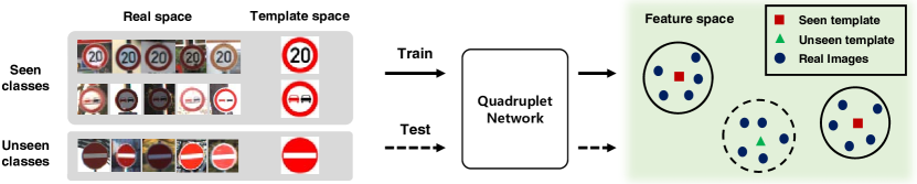
Figure 1: Illustration of a synthetic template and real image co-domain mapping.

Thus, our approach is based on the following hypotheses: 1) the existence of a co-embedding space for synthetic and real data, and 2) the existence of an embedding space where real data is condensed around a synthetic anchor for each class. We illustrate the idea in Fig. 1. Taking these into account, we learn two non-linear mappings using a neural network. The first involves mapping for a real sample into an embedding space, and the second involves mapping of a synthetic anchor onto the same metric space. We leverage the quadruplet relationship to learn non-linear mappings, which can provide rich information to learn generalized and discriminative embeddings. Classification is then performed for an embedded query point by simply finding the nearest class anchor. Despite its simplicity, our method outperforms with a margin in the unseen data regime.

Related work

Our problem can be summarized as a modified one-shot learning problem that involves heterogeneous domain datasets. This type of problem has gained little attention. Furthermore, to the best of our knowledge, our work is the first to tackle unseen traffic sign recognition with heterogeneous domain data; we therefore summarize the work most relevant to our proposed method in this section.

Non-parametric models such as nearest neighbors are useful in few-shot classification (?; ?), in that they can be naturally adapted to new data and do not require training of the model. However, the performance depends on the chosen metric (?). To overcome this, Goldberger et al. (?) propose the neighborhood components analysis (NCA) and that learns the Mahalanobis distance to maximize the accuracy of the $K$-nearest-neighbor ($K$-NN). Weinberger et al. (?), who studied large margin nearest neighbor (LMNN) classification, also maximize the $K$-NN accuracy with a hinge loss that encourages the local neighborhood of a point to contain other points with identical labels with some margin, and vice versa. Our work also adopts the hinge loss with a margin in the same spirit of Weinberger et al. Because NCA and LMNN are limited on linear model, each is extended to a non-linear model using a deep neural network in (?) and (?) respectively.

Our work may be regarded as a non-linear and quadruple extension of Mensink et al. (?) and Perrot et al. (?) to one-shot learning, in that they leverage representative auxiliary points for each class instead of individual examples of each class. These approaches are developed to adapt to new classes rapidly without re-training; however, they are designed to handle cases where novel classes come with a large number of samples. In contrast, in our scenario, a representative example is given explicitly as a template image of a traffic sign. Given such a template, we learn non-linear embedding in an end-to-end manner without pre-processing necessary in both Mensink et al. and Perrot et al. to obtain the representatives.

All of these NN classification schemes learn the metric via a pairwise relationship. In the recent metric learning literature, there have been attempts (?; ?; ?; ?; ?) to go beyond learning metrics using only a pairwise relationship (i.e., 2-tuple, e.g., Siamese (?; ?; ?)): triplet (?; ?; ?), quadruplet (?) and quintuplet (?). The use of tuples of more than a triple relationship may be inspired from the argument of Kendall and Gibbons (?), who argued that humans are better at providing relative (i.e., at least triplet-wise) comparisons than absolute comparisons (i.e., pairwise). While our method also exploits a quadruple relationship, the motivation behind this composition is rather specific for our problem definition, in which two samples from template sets and two samples from real sets have clear combinatorial pairwise relationships. More details will be described later.

Other one-shot learning approaches take wholly different notions. Koch et al. (?) uses Siamese network to classify whether two images belong to the same class. To address one-shot learning for character recognition, Late et al. (?) devise a hierarchical Bayesian generative model with knowledge of how a hand written character is created. A recent surge of models, such as a neural Turing machine (?), stimulate the meta-learning paradigm (?; ?; ?) for few-shot learning. Comparing to these works that have limited memory capacities, the NN classifier has an unlimited memory and can, automatically store and retrieve all previously seen examples. Furthermore, in the few-shot scenario, the amount of data is very small to the extent that a simple inductive bias appears to work well without the need to learn complex input-sensitive embedding (?; ?; ?), as we do so. This provides the $k$-NN with a distinct advantage.

Moreover, because we have two data sources, synthetic templates and real examples, a domain difference is naturally introduced in our problem. There is a large amount of research that smartly solves domain adaptation (refer to the survey by Csurka et al. (?) for a thorough review), but we deal with this by simply decoupling the network parameters from each other, the template and the real domains. This method is simple, but in the end it generalizes well owing to the richer back-propagation gradients from the quadruple combinations.

Quadruple network for jointly adapting domain and learning embedding

Our goal is to learn embeddings, such that different domain examples are embedded into a common metric space and where their embedded features favor to be generalized as well as discriminative.

To this end, we leverage a quadruplet relationship, consisting of two anchors of different classes and two others for examples corresponding to the anchors. We first describe the quadruple (4-tuple) construction in the following section. Subsequently, we define the embeddings followed by the objective functions and quadruplet network.

Notation We consider two imagery datasets: the template set $\mathcal{T}{=}\{(\mathbf{T},y)\}$, where each $\mathbf{T}$ denotes a representative template image and $y{\in}\{1,\dots,C\}$ is the corresponding label (out of the $C$ class), and the real example set $\mathcal{X}{=}\{\mathcal{X}_{k}\}_{k=1}^{C}$, where $\mathcal{X}_{k}$ is the set of real images $\{\mathbf{X}\}$ of class-$k$. For simplicity, we use $\mathbf{T}_{k}$ ($\mathbf{X}_{k}$) to denote a sample labeled with class-$k$.

We define Euclidean embeddings as $f(\cdot)$, where $f(\mathbf{x})$ maps a high-dimensional vector $\mathbf{x}$ into a $D$-dimensional feature space, i.e., $\mathbf{e}{=}f(\mathbf{x})\in\mathbb{R}^{D}$.

Quadruple (4-tuple) construction

Our idea is to embed template and real domain data into the same feature space such that a template sample acts as an anchor point on the feature space and real samples relevant to the anchor form a cluster around it, as illustrated in Fig. 1. Specifically, we aim to achieve two properties for an embedded feature space: 1) distinctiveness between anchors is favored, and 2) real samples must be mapped close to the anchor that corresponds to the same class.

To leverage the relational information, we define a quadruple, a basic element, by packing two template images from different classes and two real images corresponding to respective template classes, i.e., for simplicity, two classes $A$ and $B$ are considered, then $(\mathbf{T}_{A},\mathbf{T}_{B},\mathbf{X}_{A},\mathbf{X}_{B})$. From pairwise combinations within the quadruple, we can reveal several types of relational information as follows:
\raisebox{-.95pt} {1}⃝ $\mathbf{T}_{A}$ should be far from $\mathbf{T}_{B}$ in an embedding space,
\raisebox{-.95pt} {2}⃝ $\mathbf{X}_{A}$ should be far from $\mathbf{X}_{B}$ in an embedding space,
\raisebox{-.95pt} {3}⃝ $\mathbf{X}_{A}$ (or $\mathbf{X}_{B}$) should be close to $\mathbf{T}_{A}$ (or $\mathbf{T}_{B}$) in an embedding space,
\raisebox{-.95pt} {4}⃝ $\mathbf{T}_{A}$ (or $\mathbf{T}_{B}$) should be far from $\mathbf{X}_{B}$ (or $\mathbf{X}_{A}$) in an embedding space,
whereby we derive the final objective function. These relations depicted in Fig. 2(b).

Quadruple sampling

We sampled two templates $(\mathbf{T}_{A},y)$ and $(\mathbf{T}_{B},y^{\prime})$ from template set $\mathcal{T}$ while guaranteeing two different classes, followed by the two real images of $\mathbf{X}_{A}\in\mathcal{X}_{y}$ and $\mathbf{X}_{B}\in\mathcal{X}_{y^{\prime}}$.

Comparison to other tuple approaches

In metric learning, the most common approaches would be the Siamese (?; ?; ?) and triplet (?; ?; ?), which typically use 2- and 3-tuples, respectively. From the given tuple, they optimize with the pairwise differences. This concept can be viewed as follows: given a tuple, the Siamese has only a single source of loss (and its gradient), while triplets utilize two sources, i.e., (query, positive) and (query, negative). With this type of simple comparison, we can intuitively conjecture higher stability or performance of triplet network over Siamese network.

Law et al. (?) deal with a particular ambiguous quadruple relationship $(\mathsf{a}){\prec}(\mathsf{b}){\simeq}(\mathsf{c}){\prec}(\mathsf{d})$ by forcing the difference between $(\mathsf{b})$ and $(\mathsf{c})$ to be smaller than the difference between $(\mathsf{a})$ and $(\mathsf{d})$. Huang et al. (?) (quintuplet, 5-tuple) is devised a means to handle class imbalance issues by leveraging the relationships among three levels (e.g., strong, weaker and weakest in terms of a cluster analysis) of positives and negatives. Comparing the motivations of these approaches, for instance indefinite relativeness, our quadruple comes from a specific relationship, i.e., heterogeneous domain data. Moreover, it is important to note that our quadruple provides richer information (a total of $6$ pairwise information) compared to the method of Law et al. (quadruplet) which leverages a single constraint from a quadruple. It is even richer than Huang et al. (quintuplet), who provides $3$ constraints.

Quadruplet Network

Given the defined quadruple, we propose a quadruple metric learning that learns to embed template images and real images into a common metric space, say $\mathbb{R}^{D}$, through an embedding function. In order to deal with non-linear mapping, the embedding $f$ is modeled as a neural network, of which set of weight parameters are denoted as $\theta$. Since we deal with data from two different domains, template and real images, we simply use two different neural networks $\mbox{\boldmath$\theta$}_{\mathsf{T}}$ and $\mbox{\boldmath$\theta$}_{\mathsf{R}}$ for the template and real images respectively, expressed as $f_{\mathsf{T}}(\cdot){=}f(\cdot\,;\mbox{\boldmath$\theta$}_{\mathsf{T}})$ and $f_{\mathsf{R}}(\cdot){=}f(\cdot\,;\mbox{\boldmath$\theta$}_{\mathsf{R}})$, such that we can adapt both domains. Now, we are ready to define the proposed quadruple network.

The proposed quadruple network $Q$ is composed of two Siamese networks, the weights of which are shared within each pair. One part embeds features from template images and the other part for real images. Quadruple images from each domain are fed into the corresponding Siamese networks (depicted in Fig. 2(a)), and denoted as

$$Q\big{(}\left(\mathbf{T}_{A},\mathbf{T}_{B},\mathbf{X}_{A},\mathbf{X}_{B}\right);\mbox{\boldmath$\theta$}_{\mathsf{T}},\mbox{\boldmath$\theta$}_{\mathsf{R}}\big{)}$$ (1)

$$=\big{[}f_{\mathsf{T}}(\mathbf{T}_{A}),f_{\mathsf{T}}(\mathbf{T}_{B}),f_{\mathsf{R}}(\mathbf{X}_{A}),f_{\mathsf{R}}(\mathbf{X}_{B})\big{]}$$

$$=\big{[}\mathbf{e}_{\mathsf{T}}^{A},\mathbf{e}_{\mathsf{T}}^{B},\mathbf{e}_{\mathsf{X}}^{A},\mathbf{e}_{\mathsf{X}}^{B}\big{]},$$

for two different arbitrary classes $A$ and $B$, where $\mathbf{e}{\in}\mathbb{R}^{d}$ represents the embedded vector mapped by the embedding function $f$.

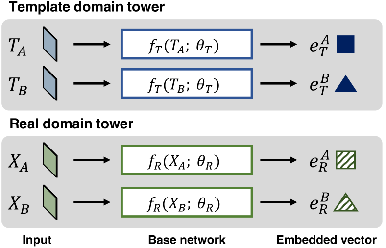
(a)

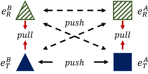
(b)

Figure 2: (a) Quadruplet network structure. (b) pairwise relations of embedded vectors.

Loss function

We mainly utilize the $l_{2}$ hinge embedding loss with a margin to train the proposed network. Given outputs quadruplet features $\big{[}\mathbf{e}_{\mathsf{T}}^{A},\mathbf{e}_{\mathsf{T}}^{B},\mathbf{e}_{\mathsf{R}}^{A},\mathbf{e}_{\mathsf{R}}^{B}\big{]}$, we have up to six pairwise relationships, as shown in Fig. 2(b)), and obtain six pairwise Euclidean feature distances as $\{d(\mathbf{e}_{\mathsf{j}}^{k},\mathbf{e}_{\mathsf{j^{\prime}}}^{k^{\prime}})\}_{j,j^{\prime}\in\{\mathsf{T},\mathsf{R}\}}^{k,k^{\prime}\in\{A,B\}}$, where $d(\mathsf{a},\mathsf{b})=\|\mathsf{a}{-}\mathsf{b}\|_{2}$ denotes the Euclidean distance. Let $h_{m}(d)$ denote the hinge loss with margin $m$ as $h_{m}(d)=\max(0,m{-}d)$, where $d$ is the distance value. We then encourage the embedded vectors with the same label pairs (i.e., if $k=k^{\prime}$) to be close by applying the loss $h_{-m}(-d)$, while pushing away the different label pairs by applying $h_{m^{\prime}}(d)$.

To induce the embedded feature space with the aforementioned two properties in the Quadruple Construction section, the minimum number of necessary losses is three, while we can exploit up to six losses; hence, we have several choices to formulate the final loss function, as described below:

$$\textsf{HingeM-3}:{L3_{m,m^{\prime}}}{=} h_{m}\left(d\left(\mathbf{e}_{\mathsf{T}}^{A},\mathbf{e}_{\mathsf{T}}^{B}\right)\right)$$ (3)

$${+}{h_{-m^{\prime}}}\left(d\left(\mathbf{e}_{\mathsf{T}}^{A},\mathbf{e}_{\mathsf{X}}^{A}\right)\right)+h_{-m^{\prime}}\left(d\left(\mathbf{e}_{\mathsf{T}}^{B},\mathbf{e}_{\mathsf{X}}^{B}\right)\right),$$

$$\textsf{HingeM-5}:{L5}_{m,m^{\prime}}{=} {L3}_{m,m^{\prime}}+h_{m}\left(d\left(\mathbf{e}_{\mathsf{T}}^{A},\mathbf{e}_{\mathsf{X}}^{B}\right)\right)$$

$$+h_{m}\left(d\left(\mathbf{e}_{\mathsf{X}}^{A},\mathbf{e}_{\mathsf{T}}^{B}\right)\right),$$

$$\textsf{HingeM-6}:{L6}_{m,m^{\prime}}{=} {L5}_{m,m^{\prime}}+h_{m}\left(d\left(\mathbf{e}_{\mathsf{X}}^{A},\mathbf{e}_{\mathsf{X}}^{B}\right)\right).$$ (4)

In addition, inspired by the contrastive loss (?), we also adopt an alternative loss by replacing the $h_{-m}(-d)$ terms in Eq. (3) with directly minimizing $d$. We denote this alternative loss simply as contrastive with a slight abuse of the terminology. We will compare these losses in the Experiments section. Analogous to traditional deep metric learning, training with these losses can be done with a simple SGD based method. By using shared parameter networks, the back-propagation algorithm updates the models w.r.t. several relationships; e.g., in the HingeM-6 case, the template tower is updated w.r.t. 5 pairwise relationships (i.e., $(\mathsf{T}^{A},\mathsf{T}^{B}),(\mathsf{T}^{A},\mathsf{X}^{A}),(\mathsf{T}^{B},\mathsf{X}^{B}),(\mathsf{T}^{A},\mathsf{X}^{B}),(\mathsf{X}^{A},\mathsf{T}^{B})$), analogously for the real tower.

Experiments

Experiment setup

Competing methods

We compare the proposed method with other deep neural network based previous works and the additionally devised baseline, as follows:

• IdsiaNet (?) is a competition winner of the German Traffic-Sign Recognition Benchmark (?) (GTSRB). We directly used an improved implementation (?). For all of the experiments, IdsiaNet is exhaustively compared as a supervised model baseline, in the same philosophy of the deep generic feature (?). Moreover, templates are not used for training. For a fair comparison, the architecture itself is adopted as the base network for the following models.

• Triplet (?) (Hoffer et al.) is similar to our model but with triplet data. Three weight shared networks are used, while in training, we randomly sampled triplets within the real image set with labels, such that no template image is exposed during triplet training. This training method is consistent with Hoffer et al.

• Triplet-DA (domain adaptation) is a variant devised by us to test our hypothesis that involving different domain templates as an anchor is beneficial. Three weight shared networks are used, and for triplet sampling, we sample one template $(\mathbf{T},y)$ from template set $\mathcal{T}$ and then sample positive and negative real images from $\mathcal{X}_{y}$ and $\mathcal{X}_{k\neq y}$ respectively.

Implementation details

For fairness, all of the details are equally applied unless otherwise specified. All input images are resized to $48{\times}48$ and the mean intensity of training set is subtracted. We did not perform any further preprocessing, data augmentation, or ensemble approach.

We use the same improved IdsiaNet (?) for the base network of Triplet, Triplet-DA and our Quadruplet, but replace the output dimension of the final layer FC2 to be $\mathbb{R}^{D}$ without a softmax layer. Every model is trained from scratch. Most of the hyper parameters are based on the implementation (?) with a slight modification (i.e., fixed learning rates: $10^{-3}$, momentum: $0.9$, weight decay: $10^{-4}$, mini-batch size: 100, optimizer: stochastic gradient descent). Models are trained until convergence is reached, i.e., $\tfrac{L_{t}-L_{t-1}}{L_{t-1}}{<}5\%$ where $L_{t}$ denotes the loss value at $t$-th iteration. We observed that the models typically converged at around $15k$-$20k$ iterations. All networks were implemented using Torch7 (?).

Dataset

We use two traffic-sign datasets, GTSRB (?) and Tsinghua-Tencent 100K (?) (TT100K). Since our motivation can be considered to involve dealing with a deficient data regime and a data imbalance caused by rare classes, we additionally introduce a subset split from GTSRB, referred to here as GTSRB-sub. To utilize the dataset properly for our evaluation schemes, given the train and test set splits provided by the authors, we further split them into seen, unseen and validation partitions, as illustrated in Fig. 3. The validation set is constructed by random sampling from the given training set. A description of the dataset construction process follows. For more details, the reader can refer to the supplementary material.

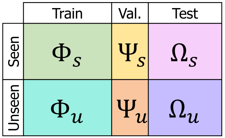
Figure 3: Partitions of dataset.

GTSRB-all GTSRB contains 43 classes. The dataset contains severe illumination variation, blur, partial shadings and low-resolution images. The benchmark provides partitions into training and test sets. The training set contains $39k$ images, where $30$ consecutively captured images are grouped, called a “track”. The test set contains $12k$ images without continuity and, thus does not form tracks. We selected 21 classes that have the fewest samples as unseen classes with the remaining 22 classes as the seen classes. Template images are involved in the dataset.

GTSRB-sub  To analyze the performance of the deficient data regime, we created a subset of GTSRB-all, forming a smaller but class-balanced training set with sharing the test set of GTSRB-all. Hence, numeric results will be compatibly comparable to that from GTSRB-all. For the training set, we randomly select 7 tracks (i.e., 210 images) for each seen classes.

TT100K-c  The TT100K detection dataset includes over 200 sign classes. We cropped traffic sign instances from the scenes to build the classification dataset (called TT100K-c). Although it contains the huge number of classes, most of the classes do not have enough instances to conduct the experiment. We only selected classes having official templates available and a sufficient number of instances. We split TT100K-c into the train and test set according to the number of instances. We set 24 classes with ${\geq}100$ instances for seen classes and select 12 unseen classes as those having $50$-$100$ instances. The training set includes half of the seen class samples, and the other half is sorted into the test set.

One-shot classification

We perform one-shot classification by 1-nearest neighbor (1-NN) classification. For 1-NN, the Euclidean distance is measured between embedding vectors by forward-feeding a query (real image) and the anchors (template images) to the network, after which the most similar anchor out of the $C$ classes is found ($C$-way classification). For the NN performance, we measure the average accuracy for each class. The seen class performance is also reported for a reference purpose.

Self-Evaluation

Table 1: Evaluations of the proposed quadruplet network with varying parameters. Evaluation is conducted on the validation set of GTSRB-all. Accuracy ($\%$) on validation set is reported.

Embedding dim ( HingeM-5 )	Top1 NN
	Avg.	Seen	Unseen
$D=50$	67.1	92.2	40.8
$D=100$	69.1	95.3	41.6
$D=150$	68.9	94.2	42.4

(a) Varying embedding dimension $d$.

Loss terms (dim 100)	Top1 NN
	Avg.	Seen	Unseen
HingeM-3	67.3	93.1	40.3
HingeM-5	69.1	95.3	41.6
HingeM-6	68.9	97.3	39.2

(b) Varying number of pairwise loss terms.

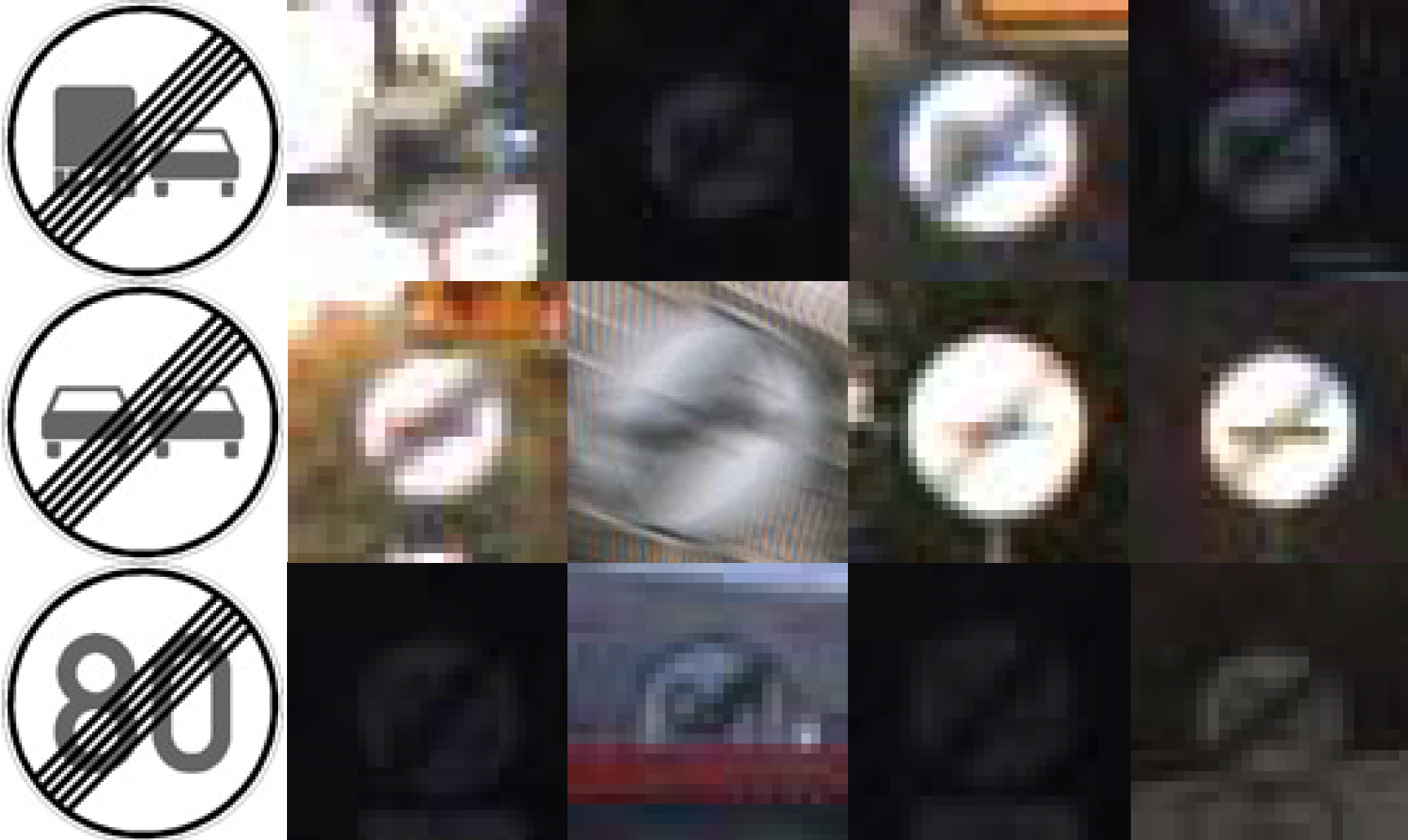
Figure 4: Some of failure cases for unseen recognition.

The proposed Quadruplet network has two main factors: the embedding dimension $D$ and the number of pairwise loss terms. We evaluate these on the validation sets $\Psi_{s}$ and $\Psi_{u}$ of GTSRB-all. The Quadruplet network is trained only with the seen training set $\Phi_{s}$.

Embedding dimension: We conduct the evaluation while varying the embedding dimension $D$, as reported in Table 1(a). We vary $D$ from $50$ to $150$ and measure the one-shot classification accuracy. We observed that the overall average accuracy across the seen and unseen classes peaked at $D{=}100$. While the unseen performance may increase further beyond $D=150$, since this sacrifices the seen performance, we select the dimension with the best average accuracy, i.e., $D=100$, as the reference henceforth.

pairwise loss terms: The quadruplet model gives 6 possible pairwise distances between outputs. Intuitively, three possible options, i.e., HingeM-3, HingeM-5 and HingeM-6 in Eqs. (3-4), satisfy our co-domain embedding property. The results in Table 1(b) show a trade-off between different losses. HingeM-3 performs worse on both seen and unseen classes than the others, while the other two have a clear trade-off. This implies that HingeM-3 is not producing enough information (i.e., gradients) to learn a good feature space. HingeM-5 outperforms Loss6 on unseen classes but HingeM-6 is better on seen classes. We suspect that complex pairwise relationships among real samples may lead to a feature space which is overly adapted to seen classes. This trade off can be used to adjust between improving the seen class performance or regularizing the model for greater flexibility. We report the following results based on HingeM-5 hereafter.

Table 2: One-shot classification (Top 1-NN) accuracy ($\%$) on the unseen classes. Performance on seen classes are shown as an additional reference.

Network type		Datasets
	Anchor	GTSRB		GTSRB subset		TT100K
		Seen	Unseen	Seen	Unseen	Seen	Unseen
IdsiaNet	$\times$	74.6	40.2	59.4	34.7	87.7	14.6
Triplet	Real	62.6	33.9	54.9	23.5	5.9	1.0
Triplet-DA	Template	86.0	54.5	60.8	47.6	86.2	67.1
Quad.+contrastive-5	Template	92.4	42.7	69.2	41.8	92.0	67.5
Quad.+hingeM	Template	90.8	45.2	70.1	47.8	94.9	67.3

Table 3: One-shot classification (Top 1-NN) accuracy ($\%$) from GTSRB-all to TT100K-c.

Network trained on GTSRB	Top1 NN
	sample average
IdsiaNet	36.5
Triplet DA	34.1
Quadruple+hingeM	42.3

Comparison to other methods

We compare the results here with those of other methods on the test sets $\Omega_{s}$ and $\Omega_{u}$ of three datasets. All networks are trained only with the seen training and validation set ${\Phi_{s}}\cup{\Psi_{s}}$ of respective datasets.

For IdsiaNet, we use the activation of FC1 for feature embedding. For the other networks, we use the final embedding vectors. For the Quadruplet network, we test two cases with contrastive-5 and HingeM-5.

Table 3 shows the results on the three datasets, where Triplet has the lowest performance, while Triplet-DA performs well. Moreover, our quadruplet network outperforms Triplet-DA in most of cases for both seen and unseen classes. This supports our hypothesis that the template (also a different domain) anchor based metric learning and the quadruplet relationship may be helpful for generalization purposes.

To check the embedding capability of each approach further, we trained each model on GTSRB ${\Phi_{s}}\cup{\Psi_{s}}$ and tested on TT100K-c ${\Omega_{s}}\cup{\Omega_{u}}$. This experiment qualifies how the networks perform on two completely different traffic sign datasets. Table 3 shows the top1-NN performance of each model. Our model performs best tn the transfer scenario, which implies that good feature representation is learned.

In order to demonstrate quantitatively the behavior of the Quadruplet network, we visualize unseen examples that are often confused by Quadruplet in Fig. 4. The unseen classes of examples that are highly similar to other classes are challenging even for humans; furthermore due to the poor illumination condition, motion blur and low resolution.

Learned representation evaluation

In this experiment, we evaluate the generalization behavior of the proposed quadruple network, which is analyzed by comparing the representation power of each network over unseen regimes (and seen class cases as a reference). In order to assess the representation quality of each method purely, we pre-train competing models and our model for ${\Phi_{s}}\cup{\Psi_{s}}$ of each dataset (i.e., only on seen classes), fix the weights of these models, and use the activations of FC1 (350 dimensions) of them as a feature. Given the features extracted by each model, we measure the representation performance by separately training the standard multi-class SVM (?) with the radial basis kernel such that the performance heavily relies on feature representation itself.

We use identical SVM parameters (nonlinear RBF kernel, $C=100,tol=0.001$) in all experiments. In contrast to FC1 trained only on seen data, the SVM model is trained on both seen and unseen classes with an equal number of instances per class, and we vary the number of per class training samples: 10, 50, 100, and 200. SVM training samples are randomly sampled from the set ${\Phi_{s}}\cup{\Psi_{s}}\cup{\Phi_{u}}\cup{\Psi_{u}}$ (Fig. 3), and the entire test set ${\Omega_{s}}\cup{\Omega_{u}}$ is used for the evaluation. We report the average score and confidence interval by repeating the experiments 100 times for the case of [No. instances$/$class: 10] and 10 times for the cases of [No. instances$/$class: 50, 100, 200]. For each sampling, we fix a random seed and test each model with the same data for a fair comparison.

With the three datasets, we show the results of the unseen ${\Omega_{u}}$ and seen ${\Omega_{s}}$ test cases in Table 4 and 5, respectively. The unseen and seen class datasets are mutually exclusive; hence, the errors should be compared in each dataset independently, e.g., the numbers in Table 4-(a) are not directly comparable with those in Table 5-(a). Instead, we can observe the algorithmic behavior difference by comparing Table 4 and 5 with respect to the relative performance.

Table 4: Feature representation quality comparison for unseen classes. SVM classification errors ($\%$) are reported with the datasets, GTSRB-all, GTSRB-sub and TT100K-c, and according to the number of SVM training instances per class. Notice that, for all the networks, the classes evaluated in this experiment are not used for training the networks, i.e., unseen classes are used only for SVM training. Marked in bold are the best results for each scenario, as well as other results with an overlapping confidence interval with 95$\%$.

Network	No. instances$/$class
	200	100	50	10
IdsiaNet	6.14 ($\pm$0.50)	6.82 ($\pm$0.57)	7.82 ($\pm$0.64)	11.01 ($\pm$0.31)
Triplet	7.22 ($\pm$0.33)	7.94 ($\pm$0.33)	8.79 ($\pm$0.40)	15.83 ($\pm$0.38)
Triplet-DA	9.04 ($\pm$0.30)	9.35 ($\pm$0.42)	10.26 ($\pm$0.63)	15.17 ($\pm$0.29)
Quad.+cont.	5.30 ($\pm$0.14)	6.09 ($\pm$0.39)	6.96 ($\pm$0.37)	9.59 ($\pm$0.23)
Quad.+hingeM	3.77 ($\pm$0.29)	3.86 ($\pm$0.27)	4.13 ($\pm$0.30)	7.69 ($\pm$0.28)

(a) GTSRB-all.

Network	No. instances$/$class
	200	100	50	10
IdsiaNet	17.89 ($\pm$0.41)	18.28 ($\pm$0.60)	18.34 ($\pm$0.79)	25.84 ($\pm$1.52)
Triplet	17.39 ($\pm$0.67)	18.22 ($\pm$0.92)	20.49 ($\pm$1.64)	30.53 ($\pm$2.47)
Triplet-DA	15.84 ($\pm$0.38)	16.77 ($\pm$0.73)	18.24 ($\pm$0.48)	28.43 ($\pm$1.61)
Quad.+cont.	12.12 ($\pm$0.33)	11.72 ($\pm$0.40)	12.83 ($\pm$0.43)	18.83 ($\pm$1.35)
Quad.+hingeM	13.81 ($\pm$0.31)	14.26 ($\pm$0.38)	15.59 ($\pm$0.52)	24.31 ($\pm$0.45)

(b) GTSRB-sub.

Network	No. instances$/$class
	20
IdsiaNet (?)	3.71 ($\pm$0.35)
Triplet (?)	3.70 ($\pm$0.30)
Triplet-DA	5.05 ($\pm$0.45)
Quad.+cont.	2.97 ($\pm$0.31)
Quad.+hingeM	2.87 ($\pm$0.24)

(c) TT100k-c.

Table 5: Feature representation quality comparison for seen classes. SVM classification errors ($\%$) are reported with the datasets, GTSRB-all, GTSRB-sub and TT100K-c, and according to the number of SVM training instances per class. Marked in bold are the best results for each scenario, as well as other results with an overlapping confidence interval with 95$\%$.

Network type	No. instances$/$class
	200	100	50	10
IdsiaNet	3.70 ($\pm$0.09)	4.24 ($\pm$0.14)	4.72 ($\pm$0.18)	6.52 ($\pm$0.10)
Triplet	5.00 ($\pm$0.08)	5.51 ($\pm$0.12)	6.22 ($\pm$0.16)	9.11 ($\pm$0.15)
Triplet-DA	4.75 ($\pm$0.12)	5.30 ($\pm$0.10)	6.08 ($\pm$0.22)	8.99 ($\pm$0.13)
Quad.+cont.	4.49 ($\pm$0.09)	4.50 ($\pm$0.12)	4.65 ($\pm$0.11)	5.61 ($\pm$0.13)
Quad.+hingeM	4.46 ($\pm$0.08)	4.63 ($\pm$0.12)	4.81 ($\pm$0.15)	5.98 ($\pm$0.08)

(a) GTSRB-all.

Network type	No. instances$/$class
	200	100	50	10
IdsiaNet	7.55 ($\pm$0.25)	8.64 ($\pm$0.22)	10.13 ($\pm$0.43)	17.19 ($\pm$0.23)
Triplet	10.88 ($\pm$0.25)	12.35 ($\pm$0.31)	14.28 ($\pm$0.27)	24.50 ($\pm$0.30)
Triplet-DA	8.78 ($\pm$0.30)	10.44 ($\pm$0.2)	12.80 ($\pm$0.37)	21.15 ($\pm$0.28)
Quad.+cont.	6.04 ($\pm$0.16)	6.88 ($\pm$0.11)	7.92 ($\pm$0.28)	12.51 ($\pm$0.21)
Quad.+hingeM	6.57 ($\pm$0.15)	7.54 ($\pm$0.23)	8.87 ($\pm$0.31)	14.02 ($\pm$0.20)

(b) GTSRB-sub.

Network type	No. instances$/$class
	20
IdsiaNet (?)	4.23 ($\pm$0.22)
Triplet (?)	5.30 ($\pm$0.14)
Triplet-DA (100)	5.53 ($\pm$0.17)
Quad.+cont.	5.39 ($\pm$0.23)
Quad.+hingeM	4.33 ($\pm$0.14)

(c) TT100k-c.

In the unseen case in Table 4, for all of the results, the proposed Quadruplet variants outperform the other competing methods, supporting the fact that our method generalizes well in limited sample regimes by virtue of the richer information from the quadruples. As an addendum, interestingly, Triplet-DA performs better than Triplet only with GTSRB-sub. We postulate that, in terms of feature description with some amount of strong supervision support, Triplet generalizes better than Triplet-DA, due inherently to the number of possible triplet combinations of Triplet-DA ($|\mathcal{T}|{\cdot}|\mathcal{X}|^{2}$, and generally $|\mathcal{T}|{\ll}|\mathcal{X}|$) is much smaller than that of Triplet due to the use of a template anchor as an element of triplet, while Triplet improves all the pairwise possibility of real data (i.e., $|\mathcal{X}|^{3}$). For the quadruplet case, more pairwise relationships results in higher number of tuple combinations and leads to better generalization, even with the use of templates.

In the seen class case in Table 5, our method and IdsiaNet show comparable performance outcomes with the best accuracy levels, while Triplet and Triplet-DA do not perform as well. We found that the proposed Quadruplet performs better than the other approaches when the number of training instances is very low, i.e., 10 samples per class. More specifically, IdsiaNet performs well in the seen class case, but not in the unseen class case compared to Quadruplet. This indicates that the embedding of IdsiaNet is trapped in seen classes rather than in general traffic sign appearances. On the other hand, the proposed method learns more general representation in that its performance in both cases is higher than those of its counterparts. We believe that this is due to the regularization effect caused by the usage of templates.

Conclusion

In this study, we have proposed a deep quadruplet for one-shot learning and demonstrated its performance on the unseen traffic-sign recognition problem with template signs. The idea is that by composing a quadruplet with a template and real examples, the combinatorial relationships enable not only domain adaptation via co-embedding learning, but also generalization to the unseen regime. Because the proposed model is very simple, it can be extended to other domain applications, where any representative anchor can be given. We think that $N>4$-tuple generalization is interesting as a future direction in that there must be a trade-off between over-fitting and memory capacities.

Supplementary Materials

Here, we present additional details of the baseline network and datasets that could not be included in the main text due to space constraints. All figures and references in this supplementary file are consistent with the main paper.

Base neural network architecture

Base network

We select the network based on classification performance under the assumption that high classification performance stems from good feature embedding capabilities. The Idsia network(?) is a winner in a German Traffic Sign Recognition Benchmark (GTSRB) competition. It was reported that variants of the Idsia network perform even better. The variant IdsiaNet uses a deeper convolution kernel size for each layer (Table 6). We use the best performing Idsia-like network  for all three embedding schemes in the experiments.

Table 6: Variant IdsiaNet structure. Zero pad 2 before each conv layers. (LCN: local contrast normalization)

Layer	Type	Size	kernel size
0	input	48x48x3	-
1	conv1	46x46x150	7x7
2	ReLU	46x46x150	-
3	Max pooling	23x23x150	2x2
4	LCN	23x23x150	7x7
5	conv2	24x24x200	4x4
6	ReLU	24x24x200	-
7	Max pooling	12x12x200	2x2
8	LCN	12x12x200	7x7
9	conv3	13x13x300	4x4
10	ReLU	13x13x300	-
11	Max pooling	6x6x300	2x2
12	LCN	6x6x300	6x6
13	fc1	350	10800 $\to$ 350
14	ReLU	350	-
15	fc2	43	350 $\to$ 43
16	softmax	43	-

Details of datasets

GTSRB-all

GTSRB (?) has been the most widely used and largest dataset for traffic-sign recognition. It contains 43 classes categorized into three super categories: prohibitory, danger and mandatory. The dataset contains illumination variations, blur, partial shadings and low-resolution images. The benchmark is partitioned into training and test sets. The training set contains 39,209 images, with 30 consecutively captured images grouped, which is referred to here at a track. The test set contains 12,630 images without continuity and thus does not form tracks. The number of samples per class varies, and the sample size also has a wide range (Fig. 6 & Fig. 7). To validate the embedding capability of the proposed model, we split the training set into two sets: seen and unseen (Fig. 5). Our motivation is to overcome the data imbalance caused by rare classes. We selected 21 classes that have the fewest samples as the unseen class, using the remaining 22 classes as the seen class. For training, we only used seen classes in the training set.

GTSRB-sub

To analyze the performance on a dataset with a limited size, we created a subset of GTSRB-all, forming a smaller size, as a class balanced training set. For the training set, we randomly selected seven tracks for each of the seen classes. For the test set, we used the same set as used in GTSRB-all; hence results will be compatible with and comparable to those of GTSRB-all.

TT100K-c

Tsinghua-Tencent 100K (?) (TT100K) is a chinese traffic sign detection dataset that includes more than 200 sign classes. We cropped traffic sign instances from scenes to build a classification dataset (called TT100K-c) to validate our model. Although it contains numerous classes, most of those in each class do not have enough instances to allow the experiment to be conducted. We only selected classes with official templates available and a sufficient number of instances. We filtered out instances that have side lengths of less than $20$ pixels, as they are unrecognizable. We split TT100K-c into the training and test set according to the number of instances. We set 24 classes that have more than 100 instances as the seen classes, and assign 12 classes with between 50 and 100 instances as the unseen class (Fig. 8). The training set includes half of the seen class samples, with the other half going to the test set. All of the unseen class samples belong to the test set. The size distribution and the number of samples per class are provided in Fig. 9 and Fig. 10, respectively.

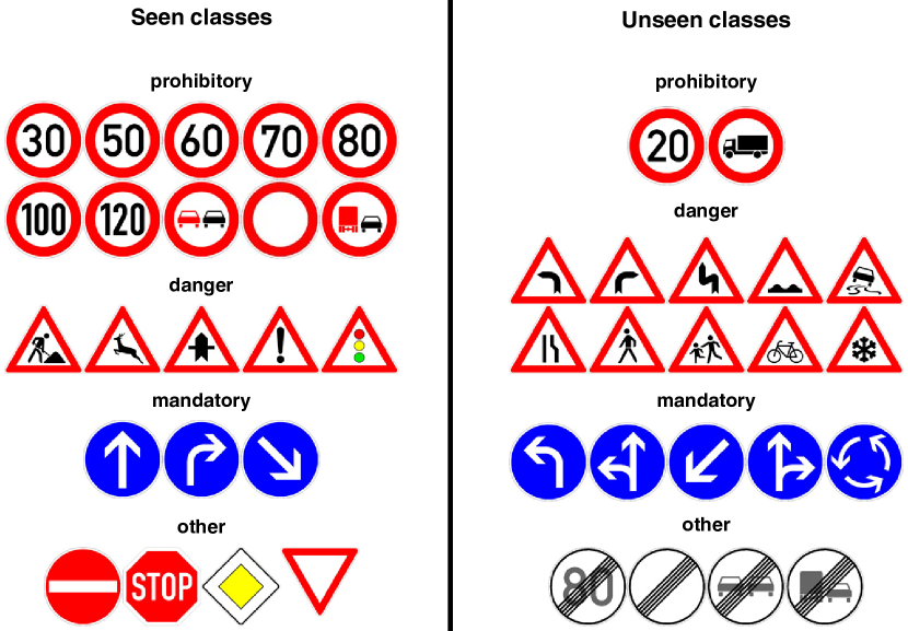
Figure 5: GTSRB template images.

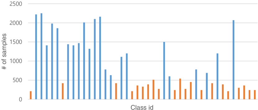
Figure 6: GTSRB class sample distribution. Blue: seen classes (#22). Orange: unseen classes (#21).

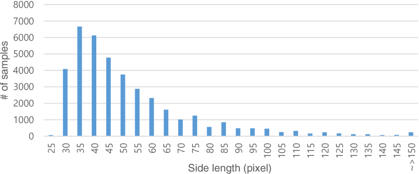
Figure 7: GTSRB size distribution. $Sidelength=(height+width)/2$

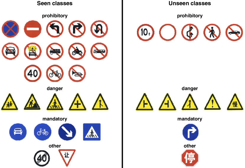
Figure 8: TT100K template images.

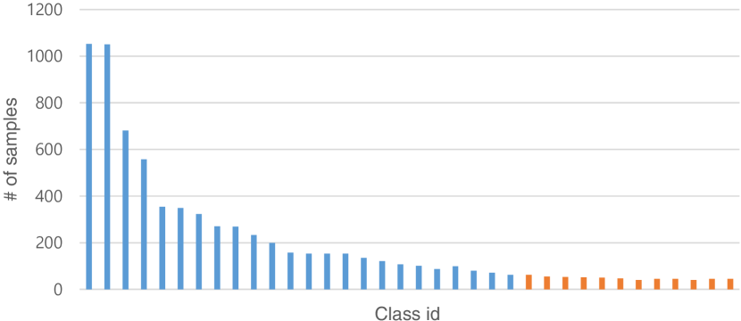
Figure 9: TT100K class sample distribution. Blue: seen classes (#24). Orange: unseen classes (#12).

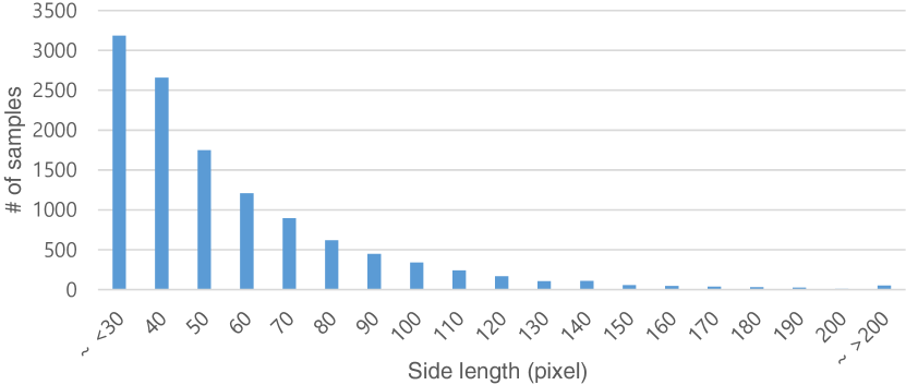
Figure 10: TT100K size distribution. $Sidelength=(height+width)/2$

References

- [Atkeson, Moore, and Schaal 1997] Atkeson, C. G.; Moore, A. W.; and Schaal, S. 1997. Locally weighted learning. Artificial Intelligence Review 11(1-5):11–73.
- [Bellet, Habrard, and Sebban 2015] Bellet, A.; Habrard, A.; and Sebban, M. 2015. Metric learning. Synthesis Lectures on Artificial Intelligence and Machine Learning 9(1):1–151.
- [Bromley et al. 1993] Bromley, J.; Guyon, I.; LeCun, Y.; Säckinger, E.; and Shah, R. 1993. Signature verification using a siamese time delay neural network. In NIPS.
- [Chang and Lin 2011] Chang, C.-C., and Lin, C.-J. 2011. Libsvm: a library for support vector machines. ACM Transactions on Intelligent Systems and Technology (TIST) 2(3):27.
- [Chen et al. 2017] Chen, W.; Chen, X.; Zhang, J.; and Huang, K. 2017. Beyond triplet loss: a deep quadruplet network for person re-identification. In CVPR.
- [Chopra, Hadsell, and LeCun 2005] Chopra, S.; Hadsell, R.; and LeCun, Y. 2005. Learning a similarity metric discriminatively, with application to face verification. In CVPR.
- [CireşAn et al. 2012] CireşAn, D.; Meier, U.; Masci, J.; and Schmidhuber, J. 2012. Multi-column deep neural network for traffic sign classification. Neural Networks 32:333–338.
- [Collobert, Kavukcuoglu, and Farabet 2011] Collobert, R.; Kavukcuoglu, K.; and Farabet, C. 2011. Torch7: A matlab-like environment for machine learning. In NIPS BigLearn Workshop.
- [Csurka 2017] Csurka, G. 2017. Domain adaptation in computer vision applications. Advances in Computer Vision and Pattern Recognition. Springer.
- [Donahue et al. 2014] Donahue, J.; Jia, Y.; Vinyals, O.; Hoffman, J.; Zhang, N.; Tzeng, E.; and Darrell, T. 2014. Decaf: A deep convolutional activation feature for generic visual recognition. In ICML.
- [Goldberger et al. 2004] Goldberger, J.; Roweis, S.; Hinton, G.; and Salakhutdinov, R. 2004. Neighbourhood components analysis. In NIPS.
- [Goodfellow, Bengio, and Courville 2016] Goodfellow, I.; Bengio, Y.; and Courville, A. 2016. Deep Learning. MIT Press.
- [Graves, Wayne, and Danihelka 2014] Graves, A.; Wayne, G.; and Danihelka, I. 2014. Neural turing machines. arXiv preprint arXiv:1410.5401.
- [Hadsell, Chopra, and LeCun 2006] Hadsell, R.; Chopra, S.; and LeCun, Y. 2006. Dimensionality reduction by learning an invariant mapping. In CVPR.
- [Hoffer and Ailon 2015] Hoffer, E., and Ailon, N. 2015. Deep metric learning using triplet network. In International Workshop on Similarity-Based Pattern Recognition, 84–92. Springer.
- [Huang et al. 2016] Huang, C.; Li, Y.; Change Loy, C.; and Tang, X. 2016. Learning deep representation for imbalanced classification. In CVPR.
- [Kendall and Gibbons 1990] Kendall, M., and Gibbons, J. D. 1990. Rank Correlation Methods. Oxford Univ.
- [Koch, Zemel, and Salakhutdinov 2015] Koch, G.; Zemel, R.; and Salakhutdinov, R. 2015. Siamese neural networks for one-shot image recognition. In ICML Deep Learning workshop.
- [Kulis and others 2013] Kulis, B., et al. 2013. Metric learning: A survey. Foundations and Trends® in Machine Learning 5(4):287–364.
- [Lake, Salakhutdinov, and Tenenbaum 2015] Lake, B. M.; Salakhutdinov, R.; and Tenenbaum, J. B. 2015. Human-level concept learning through probabilistic program induction. Science 350(6266):1332–1338.
- [Law, Thome, and Cord 2017] Law, M. T.; Thome, N.; and Cord, M. 2017. Learning a distance metric from relative comparisons between quadruplets of images. International Journal of Computer Vision (IJCV) 121:65–94.
- [Mensink et al. 2013] Mensink, T.; Verbeek, J.; Perronnin, F.; and Csurka, G. 2013. Distance-based image classification: Generalizing to new classes at near-zero cost. IEEE Transactions on Pattern Analysis and Machine Intelligence (PAMI) 35(11):2624–2637.
- [Miller, Matsakis, and Viola 2000] Miller, E. G.; Matsakis, N. E.; and Viola, P. A. 2000. Learning from one example through shared densities on transforms. In CVPR.
- [Min et al. 2009] Min, R.; Stanley, D. A.; Yuan, Z.; Bonner, A.; and Zhang, Z. 2009. A deep non-linear feature mapping for large-margin knn classification. In ICDM.
- [Perrot and Habrard 2015] Perrot, M., and Habrard, A. 2015. Regressive virtual metric learning. In NIPS.
- [Ravi and Larochelle 2017] Ravi, S., and Larochelle, H. 2017. Optimization as a model for few-shot learning. In ICLR.
- [Salakhutdinov and Hinton 2007] Salakhutdinov, R., and Hinton, G. E. 2007. Learning a nonlinear embedding by preserving class neighbourhood structure. In AISTATS.
- [Santoro et al. 2016] Santoro, A.; Bartunov, S.; Botvinick, M.; Wierstra, D.; and Lillicrap, T. 2016. Meta-learning with memory-augmented neural networks. In ICML.
- [Stallkamp et al. 2012] Stallkamp, J.; Schlipsing, M.; Salmen, J.; and Igel, C. 2012. Man vs. computer: Benchmarking machine learning algorithms for traffic sign recognition. Neural networks 32:323–332.
- [The Moodstocks team repository ] The Moodstocks team repository. Traffic sign recognition with torch. https://github.com/moodstocks/gtsrb.torch.
- [Tran et al. 2015] Tran, D.; Bourdev, L.; Fergus, R.; Torresani, L.; and Paluri, M. 2015. Learning spatiotemporal features with 3d convolutional networks. In ICCV.
- [Vinyals et al. 2016] Vinyals, O.; Blundell, C.; Lillicrap, T.; Wierstra, D.; et al. 2016. Matching networks for one shot learning. In NIPS.
- [Wang et al. 2014] Wang, J.; Song, Y.; Leung, T.; Rosenberg, C.; Wang, J.; Philbin, J.; Chen, B.; and Wu, Y. 2014. Learning fine-grained image similarity with deep ranking. In CVPR.
- [Weinberger and Saul 2009] Weinberger, K. Q., and Saul, L. K. 2009. Distance metric learning for large margin nearest neighbor classification. Journal of Machine Learning Research 10(Feb):207–244.
- [Zhu et al. 2016] Zhu, Z.; Liang, D.; Zhang, S.; Huang, X.; Li, B.; and Hu, S. 2016. Traffic-sign detection and classification in the wild. In CVPR.