Minimum Word Error Rate Training for Attention-based Sequence-to-Sequence Models

Abstract

Sequence-to-sequence models, such as attention-based models in automatic speech recognition (ASR), are typically trained to optimize the cross-entropy criterion which corresponds to improving the log-likelihood of the data. However, system performance is usually measured in terms of word error rate (WER), not log-likelihood. Traditional ASR systems benefit from discriminative sequence training which optimizes criteria such as the state-level minimum Bayes risk (sMBR) which are more closely related to WER.

In the present work, we explore techniques to train attention-based models to directly minimize expected word error rate. We consider two loss functions which approximate the expected number of word errors: either by sampling from the model, or by using N-best lists of decoded hypotheses, which we find to be more effective than the sampling-based method. In experimental evaluations, we find that the proposed training procedure improves performance by up to 8.2% relative to the baseline system. This allows us to train grapheme-based, uni-directional attention-based models which match the performance of a traditional, state-of-the-art, discriminative sequence-trained system on a mobile voice-search task.

Index Terms—  sequence-to-sequence models, attention models, minimum word error rate training, minimum Bayes risk

1 Introduction

There has been growing interest in the automatic speech recognition (ASR) community in building end-to-end trained, sequence-to-sequence models which directly output a word sequence given input speech frames, without requiring explicit alignments between the speech frames and labels. Examples of such approaches include the recurrent neural network transducer (RNN-T) [1, 2], the recurrent neural aligner (RNA) [3], attention-based models [4, 5], and connectionist temporal classification (CTC) [6] with word-based targets [7]. Such approaches are motivated by their simplicity: since these models directly output graphemes, word-pieces [8], or words, they do not require expertly curated pronunuciation dictionaries; since they can be trained to directly output normalized text, they do not require separate modules to map recognized text from the spoken to the written domain. In our recent work, we have shown that such approaches are comparable to traditional state-of-the-art speech recognition systems [9, 10].

Most sequence-to-sequence models (e.g., [4]) are typically trained to optimize the cross-entropy (CE) loss function, which corresponds to improving log-likelihood of the training data. During inference, however, model performance is commonly measured using task-specific criteria, not log-likelihood: e.g., word error rate (WER) for ASR, or BLEU score [11] for machine translation. Traditional ASR systems account for this mismatch through discriminative sequence training of neural network acoustic models (AMs) [12, 13] which fine-tunes a cross-entropy trained AM with criteria such as state-level minimum Bayes risk (sMBR) which are more closely related to word error rate.

In the context of sequence-to-sequence models, there have been a few previous proposals to optimize task-specific losses. In their seminal work, Graves and Jaitly [14] minimize expected WER of an RNN-T model by approximating the expectation with samples drawn from the model. This approach is similar to the edit-based minimum Bayes risk (EMBR) approach proposed by Shannon, which was used for minimum expected WER training of conventional ASR systems [15] and the recurrent neural aligner [3]. An alternative approach is based on reinforcement learning, where the label output at each step can be viewed as an action, so that the task of learning consists of learning the optimal policy (i.e., optimal output label sequence) which results in the greatest expected reward (lowest expected task-specific loss). Ranzato et al. [16] apply a variant of the REINFORCE algorithm [17] to optimize task-specific losses for summarization and machine translation. More recently Bahdanau et al. [18] use an actor-critic approach, which was shown to improve BLEU scores for machine translation.

In the present work, we consider techniques to optimize attention-based sequence-to-sequence models in order to directly minimize WER. Our proposed approach is similar to [14, 15] in that we approximate the expected WER using hypotheses from the model. We consider both the use of sampling-based approaches [14, 15] as well as approximating the loss over N-best lists of recognition hypotheses as is commonly done in ASR (e.g., [19]). However, unlike Sak et al. [3] we find that the process is more effective if we approximate the expectation using N-best hypotheses decoded from the model using beam-search [20] rather than sampling from the model (See section 5.1). We apply the proposed techniques on an English mobile voice-search task, to optimize grapheme-based models, with uni- and bi-directional encoders, where we find that we can improve WER by up to 8.2% relative to a CE-trained baseline model. Minimum word error rate training allows us to train grapheme-based sequence-to-sequence models which are comparable in performance to a strong state-of-the-art context-dependent (CD) phoneme-based speech recognition system [21].

The organization of the rest of the paper is as follows. We describe the particular attention-based model used in this work in Section 2 and describe the proposed approach for minimum WER training of attention models in Section 3. We describe our experimental setup and our results in Sections 4 and 5, respectively, before concluding in Section 6.

2 Attention-Based Models

We denote the set of speech utterances, suitably parameterized into feature vectors as: ${\mathbf{x}}=({\mathbf{x}}_{1},{\mathbf{x}}_{2},\cdots,{\mathbf{x}}_{T})$, where ${\mathbf{x}}_{i}\in{\mathbb{R}}^{d}$, and the corresponding ground-truth label sequence as: ${\mathbf{y}}^{*}=(y^{*}_{0},y^{*}_{1},y^{*}_{2},\cdots,y^{*}_{L+1})$, where $y^{*}_{i}\in{\mathcal{G}}$ (graphemes, in this work). We assume that the set of labels, ${\mathcal{G}}$, contains two special labels, ${\left<\texttt{sos}\right>}$ and ${\left<\texttt{eos}\right>}$, which denote the start and the end of the sentence, respectively, such that $y^{*}_{0}={\left<\texttt{sos}\right>}$ and $y^{*}_{L+1}={\left<\texttt{eos}\right>}$.

Fig. 1: The attention-based model defines a probability distribution over the next label, conditioned on the history of previous predictions: $P({\mathbf{y}}_{u}|y_{u-1},\cdots,y_{0},{\mathbf{x}})$.

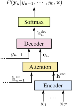
An attention-based model [4] consists of three components: an encoder network which maps input acoustic vectors into a higher-level representation, an attention model which summarizes the output of the encoder based on the current state of the decoder, and a decoder network which models an output distribution over the next target conditioned on the sequence of previous predictions: $P({\mathbf{y}}_{u}|y^{*}_{u-1},y^{*}_{u-2},\cdots,y^{*}_{0},{\mathbf{x}})$. The model is depicted in Figure 1. The encoder network consists of a deep recurrent neural network which receives as input the sequence of acoustic feature vectors, ${\mathbf{x}}$, and computes a sequence of encoded features, ${\mathbf{h}}^{\text{enc}}=({\mathbf{h}}^{\text{enc}}_{1},\cdots,{\mathbf{h}}^{\text{enc}}_{T})$, and is analogous to an acoustic model in a traditional ASR system. The decoder network - which is analogous to the pronunication and language modeling components in a traditional ASR system - consists of a deep recurrent neural network which is augmented with an attention mechanism [22]. The decoder network predicts a single label at each step, conditioned on the history of previous predictions. At each prediction step, the attention mechanism summarizes the encoded features based on the decoder state to compute a context vector, ${\mathbf{c}}_{u}$, as described in Section 2.1. The attention model thus corresponds to the component of a traditional ASR system which learns the alignments between the input acoustics and the output labels. This context vector is input to the decoder along with the previous label, $y^{*}_{u-1}$. The final decoder layer produces a set of logits which are input to a softmax layer which computes a distribution over the set of output labels: $P({\mathbf{y}}_{u}|y^{*}_{u-1},\cdots,y^{*}_{0}={\left<\texttt{sos}\right>})$.

2.1 Multi-headed Attention

The attention mechanism used in the present work differs from our previous work [10] in two important ways: firstly, we replace dot-product attention [4] with additive attention [22] which we find to be more stable; secondly, we use multiple, independent attention heads [23] allowing the model to simultaneously attend to multiple locations in the input utterance, which we find to significantly improve model performance. More specifically, we denote the recurrent hidden state of the decoder network after predicting $u-1$ labels as ${\mathbf{h}}^{\text{att}}_{u-1}$. The model employs $M$ independent attention heads, each of which computes attention values, $\beta^{i}_{t,u}\in{\mathbb{R}}$, for $1\leq i\leq M$, $1\leq t\leq T$:

$$\beta^{i}_{t,u}=\mathbf{u}^{i}\tanh(W^{i}{\mathbf{h}}^{\text{att}}_{u-1}+V^{i}{\mathbf{h}}^{\text{enc}}_{t})$$ (1)

The individual attention values are then transformed into soft attention weights through a softmax operation, and used to compute a summary of the encoder features, ${\mathbf{c}}^{i}_{u}$:

$$\alpha^{i}_{t,u}=\frac{\exp(\beta^{i}_{t,u})}{\sum_{s=1}^{T}\exp(\beta^{i}_{s,u})}\quad\quad{\mathbf{c}}^{i}_{u}=\sum_{t=1}^{T}\alpha^{i}_{t,u}Z^{i}{\mathbf{h}}^{\text{enc}}_{t}$$ (2)

The matrices $V^{i},W^{i},\text{and }Z^{i}$ and the vector, $\mathbf{u}^{i}$, are parameters of the model. Finally, the overall context vector is computed by concatenating together the individual summaries: ${\mathbf{c}}_{u}=[{\mathbf{c}}^{1}_{u};{\mathbf{c}}^{2}_{u};\cdots;{\mathbf{c}}^{M}_{u}]$.

2.2 Training and Inference

Most attention-based models are trained by optimizing the cross-entropy (CE) loss function, which maximizes the the log-likelihood of the training data:

$${\mathcal{L}}_{\text{CE}}=\sum_{({\mathbf{x}},{\mathbf{y}}^{*})}\sum_{u=1}^{L+1}-\log P(y^{*}_{u}|y^{*}_{u-1},\cdots,y^{*}_{0}={\left<\texttt{sos}\right>},{\mathbf{x}})$$ (3)

where, we always input the ground-truth label sequence during training (i.e., we do not use scheduled sampling [24]). Inference in the model is performed using a beam-search algorithm [20], where the models predictions are fed back until the model outputs the ${\left<\texttt{eos}\right>}$ symbol which indicates that inference is complete.

3 Minimum Word Error Rate Training of Attention-based Models

In this section we described how an attention-based model can be trained to minimize the expected number of word errors, and thus the word error rate. We denote by ${\mathcal{W}}({\mathbf{y}},{\mathbf{y}}^{*})$ the number of word errors in a hypothesis, ${\mathbf{y}}$, relative to the ground-truth sequence, ${\mathbf{y}}^{*}$. In order to minimize word error rates on test data, we consider as our loss function, the expected number of word errors over the training set:

$${\mathcal{L}}_{\text{werr}}({\mathbf{x}},{\mathbf{y}}^{*})=\mathbb{E}[{\mathcal{W}}({\mathbf{y}},{\mathbf{y}}^{*})]=\sum_{{\mathbf{y}}}P({\mathbf{y}}|{\mathbf{x}}){\mathcal{W}}({\mathbf{y}},{\mathbf{y}}^{*})$$ (4)

Computing the loss in (4) exactly is intractable since it involves a summation over all possible label sequences. We therefore consider two possible approximations which ensure tractability: approximating the expectation in (4) with samples [3, 15], or restricting the summation to an N-best list as is commonly done during sequence-training for ASR [19].

3.1 Approximation By Sampling

We can approximate the expectation in (4) using an empirical average over samples drawn from the model [15]:

$${\mathcal{L}}_{\text{werr}}({\mathbf{x}},{\mathbf{y}}^{*})\approx{\mathcal{L}}^{\text{Sample}}_{\text{werr}}({\mathbf{x}},{\mathbf{y}}^{*})=\frac{1}{N}\sum_{{\mathbf{y}}_{i}\sim P({\mathbf{y}}|{\mathbf{x}})}{\mathcal{W}}({\mathbf{y}}_{i},{\mathbf{y}}^{*})$$ (5)

where, ${\mathbf{y}}_{i}$ are N samples drawn from the model distribution. Critically, the gradient of the expectation in (5) can be itself be expressed as an expectation, which allows it to be approximated using samples [15]:

$$\nabla{\mathcal{L}}^{\text{Sample}}_{\text{werr}}({\mathbf{x}},{\mathbf{y}}^{*}) =\sum_{{\mathbf{y}}}P({\mathbf{y}}|{\mathbf{x}})\left[{\mathcal{W}}({\mathbf{y}},{\mathbf{y}}^{*})-\mathbb{E}[{\mathcal{W}}({\mathbf{y}},{\mathbf{y}}^{*})]\right]\nabla\log P({\mathbf{y}}|{\mathbf{x}})$$

$$\approx\frac{1}{N}\sum_{{\mathbf{y}}_{i}\sim P({\mathbf{y}}|{\mathbf{x}})}[{\mathcal{W}}({\mathbf{y}}_{i},{\mathbf{y}}^{*})-\widehat{{\mathcal{W}}}]\nabla\log P({\mathbf{y}}|{\mathbf{x}})$$ (6)

where, we exploit the fact that $\mathbb{E}[\nabla\log P({\mathbf{y}}|{\mathbf{x}})]=0$, and $\widehat{{\mathcal{W}}}=\frac{1}{N}\sum_{i=1}^{N}{\mathcal{W}}({\mathbf{y}}_{i},{\mathbf{y}}^{*})$ is the average number of word errors over the samples. Subtracting $\widehat{{\mathcal{W}}}$, serves to reduce the variance of the gradient estimates, and is important to stabilize training [15].

3.2 Approximation Using N-best Lists

One of the potential disadvantages of the sampling-based approach is that a large number of samples might be required in order to approximate the expectation well. However, since the probability mass is likely to be concentrated on the top-N hypotheses, it is reasonable to approximate the loss function by restricting the sum over just the top N hypotheses. We note that this is typically done in traditional discriminative sequence training approaches as well, where the summation is restricted to paths in a lattice [12, 13].

Denote by $\text{Beam}({\mathbf{x}},N)=\{{\mathbf{y}}_{1},\cdots,{\mathbf{y}}_{N}\}$, the set of N-best hypotheses computed using beam-search decoding [20] for the input utterance ${\mathbf{x}}$, with a beam-size, $N$. We can then approximate the loss function in (4) by assuming that the probability mass is concentrated on just the N-best hypotheses, as follows:

$${\mathcal{L}}^{\text{N-best}}_{\text{werr}}({\mathbf{x}},{\mathbf{y}}^{*})=\sum_{{\mathbf{y}}_{i}\in\text{Beam}({\mathbf{x}},N)}\widehat{P}({\mathbf{y}}_{i}|{\mathbf{x}})\left[{\mathcal{W}}({\mathbf{y}}_{i},{\mathbf{y}}^{*})-\widehat{W}\right]$$

Where, $\widehat{P}({\mathbf{y}}_{i}|{\mathbf{x}})=\frac{P({\mathbf{y}}_{i}|{\mathbf{x}})}{\sum_{{\mathbf{y}}_{i}\in\text{Beam}({\mathbf{x}},N)}P({\mathbf{y}}_{i}|{\mathbf{x}})}$, represents the distribution re-normalized over just the N-best hypotheses, and $\widehat{W}$ is the average number of word errors over the N-best hypohtheses, which is applied as a form of variance reduction, since it does not affect the gradient.

3.3 Initialization and Training

Based on the two schemes for approximating the expected word error rate, we can define two possible loss functions:

$${\mathcal{L}}^{\text{Sample}}=\sum_{({\mathbf{x}},{\mathbf{y}}^{*})}{\mathcal{L}}^{\text{Sample}}_{\text{werr}}({\mathbf{x}},{\mathbf{y}}^{*})+\lambda{\mathcal{L}}_{\text{CE}}$$ (7)

$${\mathcal{L}}^{\text{N-best}}=\sum_{({\mathbf{x}},{\mathbf{y}}^{*})}{\mathcal{L}}^{\text{N-best}}_{\text{werr}}({\mathbf{x}},{\mathbf{y}}^{*})+\lambda{\mathcal{L}}_{\text{CE}}$$ (8)

In both cases, we interpolate with the CE loss function using a hyperparameter $\lambda$ which we find is important to stabilize training (See Section 5). We note that interpolation with the CE loss function is similar to the f-smoothing approach [25] in ASR. Training the model directly to optimize ${\mathcal{L}}^{\text{Sample}}$ or ${\mathcal{L}}^{\text{N-best}}$ with random initialization is hard, since the model is not directly provided with the ground-truth label sequence. Therefore, we initialize the model with the parameters obtained after CE training.

4 Experimental Setup

The proposed approach is evaluated by conducting experiments on a mobile voice-search task. Models are trained on the same datasets as in our previous works [10, 26]. The training set consists of $\sim$15M hand-transcribed anonymized utterances extracted from Google voice-search traffic ($\sim$12,500 hours). In order to improve robustness to noise, multi-style training data (MTR) are constructed by artificially distorting training utterances with reverberation and noise drawn from environmental recordings of daily events and from YouTube using a room simulator, where the overall SNR ranges from 0-30dB with an average SNR of 12dB [27]. Model hyperparameters are tuned on a development set of $\sim$12.9K utterances ($\sim$63K words) and results are reported on a set of $\sim$14.8K utterances ($\sim$71.6K words).

The acoustic input is parameterized into 80-dimensional log-Mel filterbank features extracted over the 16kHz frequency range, computed with a 25ms window and a 10ms frame shift. Following [28], three consecutive frames are stacked together, and every third stacked frame is presented as input to the encoder. The same frontend is used for all models reported in this work.

Two attention-based models are trained in this work, differing only in the structure of the encoder network: the first model (Uni-LAS) uses 5 layers of 1,400 uni-directional LSTM cells [29], whereas the second model (Bidi-LAS) uses 5 layers of 1,024 bi-directional LSTM cells [30] (i.e., 1,024 cells in the forward and backward directions, for each layer). The decoder network of both models consists of two layers of 1,024 LSTM cells in each layer. Both models use multi-headed attention as described in Section 2.1 with $M=4$ attention heads. Models are trained to output a probability distribution over grapheme symbols: 26 lower case alphabets a-z, the numerals 0-9, punctuation symbols ,’! etc., and the special symbols ${\left<\texttt{sos}\right>}$, ${\left<\texttt{eos}\right>}$. All models are trained using the Tensorflow toolkit [31], with asynchronous stochastic gradient descent (ASGD) [32] using the Adam optimizer [33].

5 Results

We investigate the impact of various hyperparameters, and the choice of approximation scheme by conducting detailed experiments on the uni-directional LAS model. Results on the bi-directional LAS model, along with a comparison to a traditional CD-phone based state-of-the-art system are deferred until Section 5.2.

5.1 Comparison of loss functions: ${\mathcal{L}}^{\text{Sample}}$ and ${\mathcal{L}}^{\text{N-best}}$

(a) Expected number of word errors on held-out set computed using (4) when optimizing ${\mathcal{L}}^{\text{Sample}}$ as number of samples, $N$, varies.

(b) Word error rates on held-out set when optimizing ${\mathcal{L}}^{\text{Sample}}$ as a function of the number of samples, $N$.

(c) Word error rates on held-out set when optimizing ${\mathcal{L}}^{\text{N-best}}$ as a function of the depth of the N-best list, $N$.

Fig. 2: Metrics computed on held-out portion of the training set when optimizing loss functions ${\mathcal{L}}^{\text{Sample}}$ and ${\mathcal{L}}^{\text{N-best}}$, described in Section 3.3.

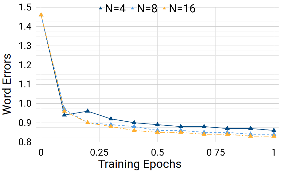
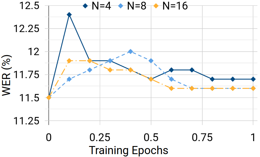
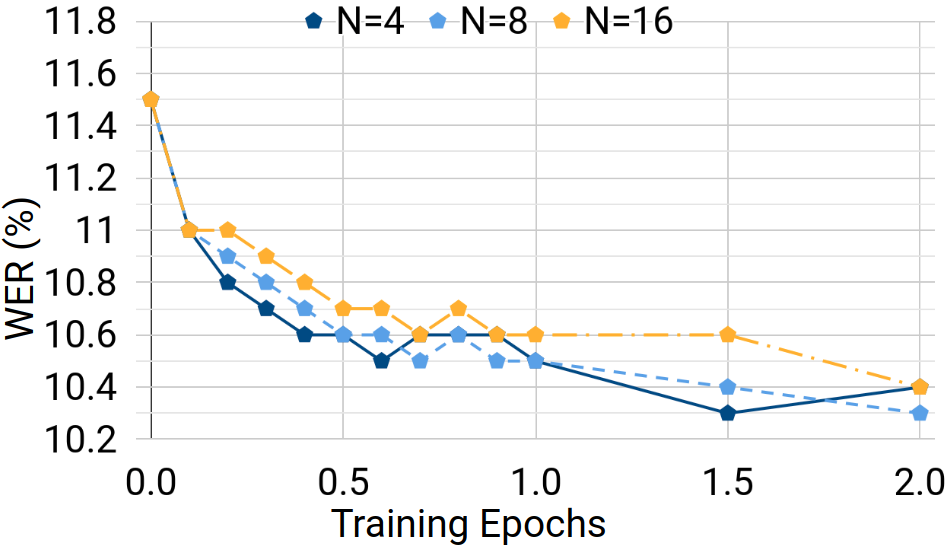
Our first set of experiments evaluate the effectiveness of approximating the expected number of word errors using samples (i.e., optimizing ${\mathcal{L}}^{\text{Sample}}$) versus the approximation using N-best lists (i.e., optimizing ${\mathcal{L}}^{\text{N-best}}$), as described in Section 3.3. Our observations are illustrated in Figure 2, where we plot various metrics on a held-out portion of the training data.

As can be seen in Figure 2(a), optimizing the sample-based approximation, ${\mathcal{L}}^{\text{Sample}}$, reduces the expected number of word errors by $\sim$50% after training, with performance appearing to improve as the number of samples, $N$, used in the approximation increases. Unlike [3], however, as can be seen in Figure 2(b), the WER for the top-hypothesis computed using beam search does not improve, but instead degrades as a result of training. We hypothesize that this is a result of the mis-match between the beam-search decoding procedure, which focuses on the head of the distribution during each next-label prediction, and the sampling procedure which also considers lower-probability paths [16].

As illustrated in Figure 2(c), optimizing ${\mathcal{L}}^{\text{N-best}}$ (i.e., using the N-best list-based approximation) significantly improves WER by about 10.4% on the held-out portion of the training set. Further, performance seems to be similar even when just the top four hypotheses are considered during the optimization.

Fig. 3: Word error rates on held-out portion of training set when optimizing ${\mathcal{L}}^{\text{N-best}}$, as a function of the CE-loss interpolation weight $\lambda$, when using $N=4$ hypotheses in the N-best list.

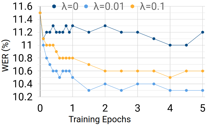
As a final note, we find that it is important to also interpolate with CE loss function during optimization (i.e., setting $\lambda>0$). This is illustrated for the case where we optimize ${\mathcal{L}}^{\text{N-best}}$ using $N=4$ hypotheses in the N-best list in Figure 3.

5.2 Improvements from Minimum WER Training for LAS Models

System	WER(%)	Rescored WER(%)
Bi-LAS	7.2	6.6
+MWER (${\mathcal{L}}^{\text{N-best}})$	6.9	6.2
Uni-LAS	8.1	7.3
+MWER (${\mathcal{L}}^{\text{N-best}})$	7.5	6.7
CD-phone (CE + sMBR)	7.5	6.7

Table 1: WERs on the test set after minimum WER training for uni- and bi-directional LAS models. The proposed procedure improves WER by up to 8.2% relative to the CE-trained baseline system.

We present results after expected minimum WER training (MWER) of the uni- and bi-directional LAS models described in Section 4 in Table 1, where we set $N=4$ and $\lambda=0.01$. We report results after directly decoding the models to produce grapheme sequences using a beam-search decoding with 8 beams (column 2) as well as after rescoring the 8-best list using a very large 5-gram language model (column 3). For comparison, we also report results using a traditional state-of-the-art low frame rate (LFR) [34] CD-phone based system, which uses an acoustic model composed of four layers of 1,024 uni-directional LSTM cells, followed by one layer of 768 uni-directional cells. The model is first trained to optimize the CE loss function, followed by discriminative sequence training to optimize the state-level minimum Bayes risk (sMBR) criterion [12]. The model is decoded using a pruned, first-pass, 5-gram language model, which uses a vocabulary of millions of words, as well as an expert-curated pronunciation dictionary. As before, we report results both before and after second-pass lattice rescoring.

As can be seen in Table 1, when decoded without second-pass rescoring (i.e., end-to-end training), MWER training improves performance of the uni- and bi-directional LAS systems by 7.4% and 4.2% respectively. The gains after MWER training are even larger after second-pass rescoring, improving the baseline uni- and bi-directional LAS systems by 8.2% and 6.1%, respectively. Finally, we note that after MWER training the grapheme-based uni-directional LAS system matches the performance of a state-of-the-art traditional CD-phoneme-based ASR system.

6 Conclusions

We described a technique for training sequence-to-sequence systems to optmize the expected test error rate, which was applied to attention-based systems. Unlike [3], we find that sampling-based approximations are not as effective as approximations based on using N-best decoded hypotheses. Overall, we find that the proposed approach allows us to improve WER by up to 8.2% relative. We find that the proposed techniques allow us to train grapheme-based sequence-to-sequence models which match performance with a traditional CD-phone-based state-of-the-art system on a voice-search task, which when viewed jointly with our previous works [10, 9] adds further evidence to the effectiveness of sequence-to-sequence modeling approaches.

References

- [1] A. Graves, “Sequence transduction with recurrent neural networks,” in In Proc. of ICML Representation Learning Workshop, 2012.
- [2] A. Graves, A-. R. Mohamed, and G. Hinton, “Speech recognition with deep neural networks,” in Proc. of ICASSP, 2013.
- [3] H. Sak, M. Shannon, K. Rao, and F. Beaufays, “Recurrent neural aligner: An encoder-decoder neural network model for sequence to sequence mapping,” in Proc. of Interspeech, 2017.
- [4] W. Chan, N. Jaitly, Q. V. Le, and O. Vinyals, “Listen, attend and spell: A neural network for large vocabulary conversational speech recognition,” in Proc. of ICASSP, 2016.
- [5] D. Bahdanau, J. Chorowski, D. Serdyuk, P. Brakel, and Y. Bengio, “End-to-end attention-based large vocabulary speech recognition,” in Proc. of ICASSP, 2016.
- [6] A. Graves, S. Fernández, F. Gomez, and J. Schmidhuber, “Connectionist temporal classificatio: Labelling unsegmented sequence data with recurrent neural networks,” in Proc. of ICML, 2006.
- [7] H. Soltau, H. Liao, and H. Sak, “Neural speech recognizer: Acoustic-to-word lstm model for large vocabulary speech recognition,” in Proc. of Interspeech, 2017.
- [8] M. Schuster and K. Nakajima, “Japanese and korean voice search,” in Proc. of ICASSP, 2012.
- [9] K. Rao, H. Sak, and R. Prabhavalkar, “Exploring architectures, data and units for streaming end-to-end speech recognition with rnn-transducer,” in Proc. of ASRU, 2017.
- [10] R. Prabhavalkar, K. Rao, T. N. Sainath, B. Li, L. Johnson, and N. Jaitly, “A comparison of sequence-to-sequence models for speech recognition,” in Proc. of Interspeech, 2017.
- [11] K. Papineni, S. Roukos, T. Ward, and W-. J. Zhu, “BLEU: A method for automatic evaluation of machine translation,” in Proc. of ACL, 2002.
- [12] B. Kingsbury, “Lattice-based optimization of sequence classification criteria for neural-network acoustic modeling,” in Proc. of ICASSP, 2009.
- [13] K. Veselỳ, A. Ghoshal, L. Burget, and D. Povey, “Sequence-discriminative training of deep neural networks.,” in Proc. of Interspeech, 2013.
- [14] A. Graves and N. Jaitly, “Towards end-to-end speech recognition with recurrent neural networks,” in Proc. of ICML, 2014.
- [15] M. Shannon, “Optimizing expected word error rate via sampling for speech recognition,” in Proc. of Interspeech, 2017.
- [16] M. Ranzato, S. Chopra, M. Auli, and W. Zaremba, “Sequence level training with recurrent neural networks,” in Proc. of ICLR, 2016.
- [17] R. J. Williams, “Simple statistical gradient-following algorithms for connectionist reinforcement learning,” Machine learning, vol. 8, no. 3-4, 1992.
- [18] D. Bahadanau, P. Brakel, R. Lowe, J. Pineau, K. Xu, A. Goyal, A. Courville, and Y. Bengio, “An actor-critic algorithm for structured prediction,” in Proc. of ICLR, 2017.
- [19] D. Povey, Discriminative Training for Large Vocabulary Speech Recognition, Ph.D. thesis, Cambridge University Engineering Department, 2003.
- [20] I. Sutskever, O. Vinyals, and Q. V. Le, “Sequence to sequence learning with neural networks,” in Proc. Of NIPS, 2014.
- [21] A. Senior, H. Sak, F. de Chaumont Quitry, T. N. Sainath, and K. Rao, “Acoustic modelling with cd-ctc-smbr lstm rnns,” in Proc. of ASRU, 2015.
- [22] D. Bahdanau, K. Cho, and Y. Bengio, “Neural machine translation by jointly learning to align and translate,” in Proc. of ICLR, 2015.
- [23] A. Vaswani, N. Shazeer, N. Parmar, L. Jones, J. Uszkoreit, A. N. Gomez, Ł. Kaiser, and I. Polosukhin, “Attention is all you need,” in Proc. of NIPS, 2017.
- [24] S. Bengio, O. Vinyals, N. Jaitly, and N. Shazeer, “Scheduled sampling for sequence prediction with recurrent neural networks,” in Proc. of NIPS, 2015.
- [25] H. Su, G. Li, D. Yu, and F. Seide, “Error back propagation for sequence training of context-dependent deep networks for conversational speech transcription,” in Proc. of ICASSP, 2013.
- [26] R. Prabhavalkar, T. N. Sainath, B. Li, K. Rao, and N. Jaitly, “An analysis of “attention” in sequence-to-sequence models,” in Proc. of Interspeech, 2017.
- [27] C. Kim, A. Misra, K. Chin, T. Hughes, A. Narayanan, T. N. Sainath, and M. Bacchiani, “Generation of large-scale simulated utterances in virtual rooms to train deep-neural networks for far-field speech recognition in google home,” in Proc. of Interspeech, 2017.
- [28] H. Sak, A. Senior, K. Rao, and F. Beaufays, “Fast and accurate recurrent neural network acoustic models for speech recognition,” in Proc. of Interspeech, 2015.
- [29] S. Hochreiter and J. Schmidhuber, “Long short-term memory,” Neural Computation, vol. 9, no. 8, pp. 1735–1780, Nov 1997.
- [30] M. Schuster and K. K. Paliwal, “Bidirectional recurrent neural networks,” IEEE Transactions on Signal Processing, vol. 45, no. 11, pp. 2673–2681, Nov 1997.
- [31] M. Abadi, A. Agarwal, P. Barham, E. Brevdo, Z. Chen, C. Citro, G. Corrado, A. Davis, J. Dean, M. Devin, S. Ghemawat, I. Goodfellow, A. Harp, G. Irving, M. Isard, Y. Jia, R. Jozefowicz, L. Kaiser, M. Kudlur, J. Levenberg, D. Mané, R. Monga, S. Moore, D. Murray, C. Olah, M. Schuster, J. Shlens, B. Steiner, I. Sutskever, K. Talwar, P. Tucker, V. Vanhoucke, V. Vasudevan, F. Viégas, O. Vinyals, P. Warden, M. Wattenberg, M. Wicke, Y. Yu, and X. Zheng, “Tensorflow: Large-scale machine learning on heterogeneous distributed systems,” 2015.
- [32] B. Recht, C. Re, S. Wright, and F. Niu, “Hogwild: A lock-free approach to parallelizing stochastic gradient descent,” in Proc. of NIPS, 2011.
- [33] D. P. Kingma and J. Ba, “Adam: A method for stochastic optimization,” in Proc. of ICLR, 2015.
- [34] G. Pundak and T. N. Sainath, “Lower frame rate neural network acoustic models,” in Proc. of Interspeech, 2016.