Improving the Performance of Online Neural Transducer Models

Abstract

Having a sequence-to-sequence model which can operate in an online fashion is important for streaming applications such as Voice Search. Neural transducer is a streaming sequence-to-sequence model, but has shown a significant degradation in performance compared to non-streaming models such as Listen, Attend and Spell (LAS). In this paper, we present various improvements to NT. Specifically, we look at increasing the window over which NT computes attention, mainly by looking backwards in time so the model still remains online. In addition, we explore initializing a NT model from a LAS-trained model so that it is guided with a better alignment. Finally, we explore including stronger language models such as using wordpiece models, and applying an external LM during the beam search. On a Voice Search task, we find with these improvements we can get NT to match the performance of LAS.

1 Introduction

Sequence-to-sequence models have become popular in the automatic speech recognition (ASR) community [1, 2, 3, 4], as they allow for one neural network to jointly learn an acoutic, pronunciation and language model, greatly simplifying the ASR pipeline. In this paper, we focus on attention-based sequence-to-sequence models, as our previous study [5] showed these models performed better than alternatives such as Connectionist Temporal Classification (CTC) [6] and Recurrent Neural Network Transducer (RNN-T) [7].

Attention-based models consist of three modules. First, an encoder, represented by a multi-layer recurrent neural network (RNN), models the acoustics. Second, a decoder, which consists of multiple RNN layers, predicts the output sub-word unit sequence. Finally, an attention layer selects frames in the encoder representation that the decoder should attend to when predicting each sub-word unit.

Attention-based models, such as Listen, Attend and Spell (LAS) have typically been explored in “full-sequence” mode, meaning attention is computed by seeing the entire input sequence [2, 4]. Thus, during inference, the model can produce the first output token only after all input speech frames have been consumed. While such a mode of operation might be suitable for many applications, these models cannot be used for “streaming” speech recognition, such as voice search, where the output text should be generated as soon as possible after words are spoken [8].

Recently, neural transducer (NT) [3] was proposed as a limited-sequence streaming attention-based model, which consumes a fixed number of input frames (a chunk), and outputs a variable number of labels before it consumes the next chunk. While the model is attractive for streaming applications, in previous work NT showed a large degradation over other online sequence-to-sequence models such as RNN-T [9] and full-sequence unidirectional attention-based models [3, 4], particularly as the chunk-size was decreased [4].

In the present work, we study various improvments to the streaming NT model – both in terms of model structure, as well as in the training procedure – that are aimed at improving its performance to be as close as possible to the non-streaming full-sequence unidirectional LAS model, which serves as an upper-bound of sorts. Specifically, we allow attention in NT to be computed looking back many previous chunks, as this does not introduce additional latency. Further, we find that allowing the model to look-ahead by 5 frames is extremely beneficial. Finally, we allow NT to be initialized from a pre-trained LAS model, which we find is a more effective strategy than having the model learn from scratch.

Our NT experiments are conducted on a 12,500 hour Voice Search task. We find that with look-back and look-ahead, NT is more than 20% relative worse than LAS in terms of word error rate (WER). However, we find that by pretraining with LAS, we can get NT with a chunk size of 10 (450ms latency) to match the performance of LAS, but a chunk size of 5 (300ms latency) still degrages by 3% relative.

Our analysis of the NT model indicates that many of the errors made compared to LAS are language modeling (LM) errors. Thus, we explore various ideas to incorporate a stronger language model (LM) into NT, to allow us to reduce the chunk size. This includes exploring incorporating an LM from the encoder side via multi-head attention, training the NT model with word pieces [10] to get a stronger LM into the decoder [11] and also explicitly incorporating an external LM via shallow fusion [12]. We find that our best performing NT system with a chunk size of 5 (300 ms latency) only degrades performance by 1% relative to an unidirectional LAS system.

2 Original Neural Transducer Algorithm

In this section, we describe the basic NT model introduced in Jaitly et al. [3]. which is shown in Figure 1. Given an input sequence of frame-level features (e.g., log-mel-filterbank energies), $\mathbf{x}=\{x_{1},x_{2},\ldots,x_{T}\}$, and an output sequence of sub-word units (e.g., graphemes, or phonemes) $\mathbf{y}=\{y_{1},y_{2},\ldots y_{N}\}$, attention models assume that the probability distribution of each sub-word unit is conditioned on the previous history of sub-word unit predictions, $y_{<i}$, and the input signal. Full-sequence attention models, such as LAS [2] compute the probability of the output prediction $y_{<i}$ for each step $i$ given the entire input acoustic sequence $\mathbf{x}$, making it unsuitable for streaming recognition applications. The Neural Transducer (NT) model [3] is a limited-sequence attention model that addresses this issue by limiting attention to fixed-size blocks of the encoder space.

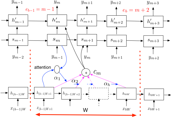
Fig. 1: Neural Transducer Attention Model.

Given the input sequence, $\mathbf{x}$, of length $T$, and a block size of length $W$, the input sequence is divided equally into blocks of length $B=\lceil{\frac{T}{W}}\rceil$, except for the last block which might contain fewer than $B$ frames. The NT model examines each block in turn, starting with the left-most block (i.e., the earliest frames). In this model, attention is only computed over the frames in each block. Within a block, the NT model produces a sequence of $k$ outputs, $y_{i},\ldots,y_{i+k}$; it is found to be useful to limit the maximum number of outputs that can be produced within a block to $M$ symbols, so that $0\leq k\leq M$. Once it has produced all of the required labels within a block, the model outputs an <epsilon> symbol, which signifies the end of block processing. The model then proceeds to compute attention over the next block, and so on, until all blocks have been processed. The <epsilon> symbol is analogous to the blank symbol in connectionist temporal classification (CTC) [6]. In particular, we note that a block must output a minimum of one symbol (<epsilon>), before proceeding to the next block.

The model computes $P(y_{1,\ldots,(S+B)}|\mathbf{x}_{1\ldots T})$, which outputs a sequence which is length $B$ longer than the LAS model since the model must produce an <epsilon> at every block. Within each block $b\in B$, the model computes the following probability in Equation 1, where $y_{e_{b}}=\texttt{<epsilon>}$ is the symbol at the end of each block. In other words, the prediction $y_{i}$ at the current step, $i$, is based on the previous predictions $y_{1\ldots{e_{(i-1)}}}$, similar to LAS, but in this case using acoustic evidence only up to the current block, $\mathbf{x}_{1\ldots bW}$:

$$P(y_{(e_{b-1}+1)\ldots e_{b}}|\mathbf{x}_{1\ldots bW},y_{1\ldots{e_{b-1}}})=\\ \prod_{i=e_{(b-1)}+1}^{e_{b}}P(y_{i}|\mathbf{x}_{1\ldots bW},y_{1\ldots{e_{(i-1)}}})$$ (1)

Like LAS, NT also consists of a listener, an attender and a speller to define a probability distribution over the next sub-word unit conditioned on the acoustics and the sequence of previous predictions. The listener module of the NT computes an encoding vector in the current block only:

$$\mathbf{h}_{(b-1)W+1\ldots bW}=\text{Listen}(\mathbf{x}_{(b-1)W+1\ldots bW})$$ (2)

which is implemented as a unidirectional RNN.

The goal of the attender and speller is to take the output of the listener (i.e., $\mathbf{h}$) and produce a probability distribution over sub-word units. The attention and speller modules operate similar to LAS, but only work on the partial output, $\mathbf{h}_{1\ldots bW}$, of the encoder up until the current block. We refer the reader to [4] for more details about the attention and speller.

3 Improving Performance of Basic Neural Transducer Algorithm

In this section, we describe various improvements to the basic algorithm and model described in the previous section.

3.1 Training grapheme-based models using Word Alignments

Training with NT requires knowing which sub-word units occur in each chunk, and thus an alignment is needed. Our previous work with NT [4] used context-independent phonemes, for which an alignment was available. In this work, we train our model with graphemes, which does not have an alignment. However, we have a word level alignment and we use this information to emit all graphemes in the chunk corresponding to when a word has finished.

3.2 Extending Attention Range

In the original NT paper, attention was computed by only looking at encoder features in the current block $b$, as shown in Equation 2. However, as shown in [4], making the attention window longer allows NT to approach the performance of LAS, but at the cost of removing the online nature of the task. However, we can still maintain a streaming, online system by computing attention by looking back over $k$ previously blocks. This is particularly important because we emit graphemes at word boundaries. Furthermore, similar to our streaming systems [13], we allow a lookahead of 150 ms (5 30-ms frames) between the input frames and the output prediction. With these changes, the listener is now shown by Equation 3.

$$\mathbf{h}_{(b-1)W+1\ldots bW}=\text{Listen}(\mathbf{x}_{(b-k)W+1\ldots bW+5})$$ (3)

3.3 Pre-training with LAS

Attention-based models learn an alignment (represented via an attention vector), jointly with the acoustic model (encoder) and language model (decoder). One hypothesis we have for NT lagging behind LAS is that during training, the attention mechanism is limited in the window over which it can compute attention. This problem is exacerbated by the fact that we emit graphemes only at word boundaries.

However, we can see from attention plots in LAS [2] that once the attention mechanism is learned, it appears to be fairly monotonic. Since NT and LAS are parameterized exactly the same (except for an extra <epsilon> output target), we can train a LAS model with this extra target (which is ignored as it does not appear in the LAS target sequence) and used it to initialize NT. Our intuition is that since LAS learns a good attention mechanism that is relatively monotonic, it can be used to initialize NT and NT will not take a large hit in accuracy compared to LAS.

3.4 Incorporating a Stronger Language Model

As we make the chunk-size smaller, looking at the errors it appears that most of the errors are due to language modeling errors. Therefore, we explore if we can incorporate a stronger LM into the decoding and/or training process.

3.4.1 Wordpiece Models

To increase the memory and linguistic span of the decoder, we emit wordpieces instead of graphemes [14]. In this approach, words a broken up, deterministically, into sub-word units, called wordpieces. For instance, the phrase “Jet makers feud” can be broken up into (“_J” , “et”, “_makers”, “_fe”, “ud”) some words may be broken down into sub-units while common words (“makers”) are modeled as a single unit. Wordpieces are position-dependent, so we mark the beginning of each word with a special marker “_”. The wordpiece inventory is trained to maximize the likelihood of the training text. Wordpieces achieve a balance between the flexibility of characters and efficiency of words.

Sequence-to-sequence models that predict wordpieces have been successful in both machine translation [14] and speech [11, 15]. Since these models are trained to predict wordpieces, rather than graphemes, a much stronger decoder LM is used. We hypothesize that by predicting wordpieces, we can reduce chunk size as well with NT.

3.4.2 Incorporating external LM

Language models have been successfully incorporated into sequence-to-sequence models to guide the beam search to output a more likely set of candidates [16, 17]. In this work, we explore if incorporating an external LM into the beam search can aid NT. Following a similar approach to [16, 18], we look at doing a log-linear interpolation between the LAS model and an FST-based LM trained to go from graphemes to words at each step of the beam search, also known as shallow fusion [17]. In this equation $p(\mathbf{y}|\mathbf{x})$ is the score from the LAS model, which is combined with a score coming from an external LM $p_{LM}(\mathbf{x})$ weighted by an LM weight $\lambda$, and a coverage term to promote longer transcripts [16] and weighted by $\eta$.

$$\mathbf{y}^{*}=\arg\min_{y}-\log p(\mathbf{y}|\mathbf{x})-\lambda\log p_{LM}(\mathbf{x})-\eta\texttt{coverage}\vspace{-0.1in}$$ (4)

4 Experimental Details

Our experiments are conducted on a $\sim$12,500 hour training set consisting of 15 million English utterances. The training utterances are anonymized and hand-transcribed, and are representative of Google’s voice search traffic. This data set is created by artificially corrupting clean utterances using a room simulator, adding varying degrees of noise and reverberation such that the overall SNR is between 0dB and 30dB, with an average SNR of 12dB [19]. The noise sources are from YouTube and daily life noisy environmental recordings. We report results on a set of $\sim$14,800 anonymized, hand-transcribed Voice Search utterances extracted from Google traffic.

All experiments use 80-dimensional log-mel features, computed with a 25-ms window and shifted every 10ms. Similar to [13, 20], at the current frame, $t$, these features are stacked with 2 frames to the left and downsampled to a 30ms frame rate. The encoder network architecture consists of 5 unidirectional long short-term memory [21] (LSTM) layers, with the size specified in the results section. Additive attention is used for all experiments [22]. The decoder network is a 2 layer LSTM with 1,024 hidden units per layer. All networks are trained to predict 74 graphemes unless otherwise noted.

All neural networks are trained with the cross-entropy criterion, using asynchronous stochastic gradient descent (ASGD) optimization [23] with Adam [24] and are trained using TensorFlow [25].

5 Results

5.1 Getting NT To Work Online

5.1.1 Attention Window

Our first set of experiments analyzes the behavior of NT as we vary the window used to compute attention. For these experiments, we use an encoder which consists of five layers of 768 uni-directional LSTM cells and a decoder with two layers of 768 LSTM cells. As can be seen in Table 1, when we only allow the NT model to compute attention within a chunk of size 10, performance is roughly 25% worse in terms of WER compared to the LAS model which differs only in the window over which attention is computed. Allowing the model to compute attention over the last 20 chunks in addition to the current chunk, however, slightly improves performance of the NT system. Finally, if we allow a 5 frame look-ahead , the results improve but NT is still roughly 13% relative worse compared to LAS. Based on the results in Table 1, since the proposed changes improve performance, all future NT results in the paper use a look-back of 20 chunks and a look-ahead of 5 frames.

System	Chunk Size	WER
LAS	-	11.7
NT, attention within chunk	10	14.6
NT, look back	10	14.4
+ look ahead	10	13.2

Table 1: WER for NT, Varying Chunks Looked Over

5.1.2 Initialization from LAS, Single-head attention

Next, we analyze the behavior of NT, for both a chunk size of 5 and 10, when we pretrain with LAS. For these experiments, we compare two different encoder/decoder sizes. Table 2 shows that when NT is pre-trained with LAS, at a chunk size of 10 (i.e., 450 ms latency) we can match the performance of LAS. However, a chunk size of 5 (300ms latency), which is our requirement for allowed streaming delay, still lags behind LAS by 3% relative for the larger model.

System	Chunk	5x768	5x1024
		2x768	2x1024
LAS	-	11.7	9.8
NT, scratch	10	13.2	11.1
NT, pretrained	10	11.4	9.9
NT, scratch	5	-	14.5
NT, pretrained	5	-	10.1

Table 2: WER for NT, Pretrained from LAS

5.1.3 Initialization from LAS, Multi-head attention

LAS, MHA	NT-Ch5, MHA	NT-Ch5, MHA, WPM
school closing in	what closing in	school closing in
parma for tomorrow	parma for tomorrow	parma for tomorrow
how to multiply two	how to multiply two	how to multiply two
numbers with decimals	numbers with this most	numbers with decimals
how far is it from albuquerque new	how far is it from albuquerque new	how far is it from albuquerque new
mexico to fountain hills arizona	mexico to to fountain hills arizona	mexico to fountain hills arizona
is under the arm warmer or colder	is under the arm warmer or colder	is under the arm warmer or colder
than in mouth temperature	than a mouse temperature	than in mouth temperature

Table 3: Representative errors made by different systems, indicated in red.

Next, we compare the behavior of LAS vs. NT when the system uses multi-head attention [26], which has been shown to give state-of-the-art ASR performance for LAS [27]. The MHA model uses a 5x1400 encoder with 4 attention heads, and a 2x1024 decoder. Table 4 shows that the performance of NT does not improve from single to multi-head attention, even though the LAS system does. One hypothesis is that multi-head attention computes attention from multiple points in the encoder space that come after the current prediction, which are ignored by streaming models such at NT.

System	Chunk	Single Attention - WER	MHA - WER
		5x1024,2x1024	5x1400,2x1024
LAS	-	9.8	8.0
NT	10	9.9	9.8
NT	5	10.1	10.3

Table 4: WER for NT with MHA

To understand the loss in performance caused by NT compared to LAS, we analyzed sentences where LAS was correct and NT incorrect, denoted in the first two columns of Table 3 as “LAS-MHA” and “NT-Ch5,MHA”. The table shows that a lot of the NT errors are due to language modeling errors. In the next section, we look at a few simple ways of incorporating an LM into the system.

5.2 Incorporating the LM

5.2.1 Wordpieces

Our next set of results looks at incorporating wordpieces into the LAS and NT models, which provide a stronger LM from the decoder side. For these experiments, we used 32,000 wordpieces. Table 5 shows that with wordpieces, the NT and LAS models are now much closer compared to graphemes. In addition, there is very little difference between NT with a chunk size of 5 and 10. One hypothesis is that since wordpieces are now longer units, each attention head focused on by neural transducer corresponds to a much longer subword unit (potentially a word) compared to the NT grapheme MHA system. Therefore, the MHA WPM feeds a much stronger set of context vectors to the decoder compared to NT grapheme model. This can also be visually observed by looking at the attention plots for the grapheme vs. wordpiece systems in Figure 2. The plot shows that the attention vectors for wordpieces span a much longer left context window compared to graphemes.

System	Chunk	WER
LAS	-	8.6
NT	10	8.6
NT	5	8.7

Table 5: WER for NT with MHA + WPM

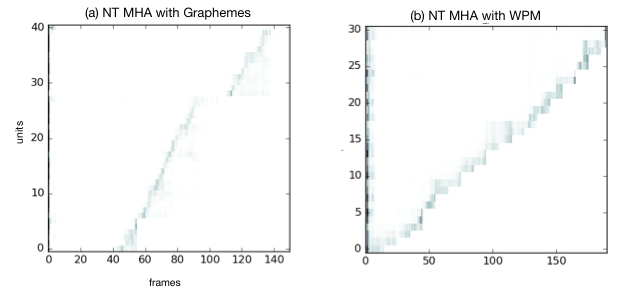
Fig. 2: Attention Plots for NT-MHA with (a) Graphemes, (b) WPM. The two attention plots also correspond to different utterances.

5.2.2 WPM + LM

Finally, we investigate incorporating an external LM into the MHA+WPM LAS and NT models. In these experiments, a n-gram FST LM, trained on 32K wordpieces, is used. This LM is trained on 1 billion text queries, a much larger set compared to the 15 million utterances seen by the LAS/NT models. Table 6 shows the the FST LM does not give any additional improvement for both NT and LAS. It has been observed in [18] that the perplexity of a WPM RNN-LM is much lower than a WPM FST. Since the decoder of the LAS and NT models is an RNN-LM, it is possible there is nothing more to gain by incorporating the WPM FST. In the future, we will repeat this with a WPM RNN-LM trained on text data.

System	Chunk	No LM	with LM
LAS	-	8.6	8.6
NT	10	8.6	8.6
NT	5	8.7	8.7

Table 6: WER for NT, Incorporating External LM

Finally, it should be noted that after including both WPM and external LM, the last column of Table 3, namely “NT-Ch5,MHA,WPM” illustrates that many of the previous sentences are now fixed and match the LAS hypothesis. With the proposed LM improvements, NT with a chunk size of 5 has comparable performance to LAS, while meeting the allowable delay of 300ms.

6 Conclusions

In this paper, we presented various improvements to NT. Specifically, we showed we could improve performance by increasing the attention window and pre-training NT with LAS. With these improvements, a single-head NT model could come very close to the performance of LAS while a multi-head attention NT model still degraded over LAS. By incorporating a stronger LM through wordpieces, multi-head NT could effetively match the performance of LAS.

7 Acknowledgements

The authors would like to thank Navdeep Jaitly, Michiel Bacchiani and Gabor Simko for helpful discussions.

References

- [1] J. K. Chorowski, D. Bahdanau, D. Serdyuk, K. Cho, and Y. Bengio, “Attention-Based Models for Speech Recognition,” in Proc. NIPS, 2015.
- [2] W. Chan, N. Jaitly, Q. V. Le, and O. Vinyals, “Listen, attend and spell,” CoRR, vol. abs/1508.01211, 2015.
- [3] N. Jaitly, D. Sussillo, Q. V. Le, O. Vinyals, I. Sutskever, and S. Bengio, “An Online Sequence-to-sequence Model Using Partial Conditioning,” in Proc. NIPS, 2016.
- [4] R. Prabhavalkar, T. N. Sainath, B. Li, K. Rao, and N. Jaitly, “An Analysis of ”Attention” in Sequence-to-Sequence Models,” in Proc. Interspeech,” in Proc. Interspeech, 2017.
- [5] R. Prabhavalkar, K. Rao, T. N. Sainath, B. Li, L. Johnson, and N. Jaitly, “A Comparison of Sequence-to-sequence Models for Speech Recognition,” in Proc. Interspeech, 2017.
- [6] A. Graves, S. Fernandez, F. Gomez, and J. Schmidhuber, “Connectionist Temporal Classification: Labeling Unsegmented Sequenece Data with Recurrent Neural Networks,” in Proc. ICML, 2006.
- [7] A. Graves, “Sequence transduction with recurrent neural networks,” CoRR, vol. abs/1211.3711, 2012.
- [8] M. Shannon, G. Simko, S. Chan, and C. Parada, “Improved End-of-Query Detection for Streaming Speech Recognition,” .
- [9] E. Battenberg, J. Chen, R. Child, and A. Coates et. al., “Exploring Neural Transducers for End-to-End Speech Recognition,” in Proc. ASRU, 2017.
- [10] Mike Schuster and Kaisuke Nakajima, “Japanese and Korean voice search,” 2012 IEEE International Conference on Acoustics, Speech and Signal Processing, 2012.
- [11] K. Rao, R. Prabhavalkar, and H. Sak, “Exploring Architectures, Data and Units for Streaming End-to-End Speech Recognition with RNN-Transducer,” in Proc. ASRU, 2017.
- [12] J. K. Chorowski and N. Jaitly, “Towards Better Decoding and Language Model Integration in Sequence to Sequence Models,” in Proc. Interspeech, 2017.
- [13] G. Pundak and T. N. Sainath, “Lower Frame Rate Neural Network Acoustic Models,” in Proc. Interspeech, 2016.
- [14] Y. Wu, M. Schuster, and et. al., “Google’s neural machine translation system: Bridging the gap between human and machine translation,” CoRR, vol. abs/1609.08144, 2016.
- [15] William Chan, Yu Zhang, Quoc Le, and Navdeep Jaitly, “Latent Sequence Decompositions,” in ICLR, 2017.
- [16] J. Chorowski and N. Jaitly, “Towards Better Decoding and Language Model Integration in Sequence to Sequence Models,” in Proc. Interspeech, 2017.
- [17] A. Sriram, H. Jun, S. Satheesh, and A. Coates, “Cold fusion: Training seq2seq models together with language models,” CoRR, vol. abs/1708.06426, 2017.
- [18] A. Kannan, Y. Wu, P. Nguyen, T. N. Sainath, Z. Chen, and R. Prabhavalkar, “An analysis of incorporating an external language model into a sequence-to-sequence model,” in submitted to Proc. ICASSP, 2018.
- [19] C. Kim, A. Misra, K. Chin, T. Hughes, A. Narayanan, T. N. Sainath, and M. Bacchiani, “Generated of large-scale simulated utterances in virtual rooms to train deep-neural networks for far-field speech recognition in google home,” in Proc. Interspeech, 2017.
- [20] H. Sak, A. Senior, K. Rao, and F. Beaufays, “Fast and Accurate Recurrent Neural Network Acoustic Models for Speech Recognition,” in Proc. Interspeech, 2015.
- [21] S. Hochreiter and J. Schmidhuber, “Long Short-Term Memory,” Neural Computation, vol. 9, no. 8, pp. 1735–1780, Nov 1997.
- [22] D. Bahdanau, K. Cho, and Y. Bengio, “Neural Machine Translation by Jointly Learning to Align and Translate,” CoRR, vol. abs/1409.0473, 2014.
- [23] J. Dean, G.S. Corrado, R. Monga, K. Chen, M. Devin, Q.V. Le, M.Z. Mao, M. Ranzato, A. Senior, P. Tucker, K. Yang, and A.Y. Ng, “Large Scale Distributed Deep Networks,” in Proc. NIPS, 2012.
- [24] D. P. Kingma and J. Ba, “Adam: A method for stochastic optimization,” in Proc. of ICLR, 2015.
- [25] M. Abadi et al., “TensorFlow: Large-Scale Machine Learning on Heterogeneous Distributed Systems,” Available online: http://download.tensorflow.org/paper/whitepaper2015.pdf, 2015.
- [26] A. Vaswani, N. Shazeer, N. Parmar, J. Uszkoreit, L. Jones, A. N. Gomez, L. Kaiser, and I. Polosukhin, “Attention Is All You Need,” CoRR, vol. abs/1706.03762, 2017.
- [27] C. Chen, T. N. Sainath, Y. Wu, R. Prabhavalkar, P. Nguyen, Z. Chen, A. Kannan, R. J. Weiss, K. Rao, N. Jaitly, B. Li, and J. Chorowski, “State-of-the-art speech recognition with sequence-to-sequence models,” in submitted to Proc. ICASSP, 2018.