Estimating linear functionals of a sparse family of Poisson means

Abstract

Assume that we observe a sample of size $n$ composed of $p$-dimensional signals, each signal having independent entries drawn from a scaled Poisson distribution with an unknown intensity. We are interested in estimating the sum of the $n$ unknown intensity vectors, under the assumption that most of them coincide with a given “background” signal. The number $s$ of $p$-dimensional signals different from the background signal plays the role of sparsity and the goal is to leverage this sparsity assumption in order to improve the quality of estimation as compared to the naive estimator that computes the sum of the observed signals. We first introduce the group hard thresholding estimator and analyze its mean squared error measured by the squared Euclidean norm. We establish a nonasymptotic upper bound showing that the risk is at most of the order of $\sigma^{2}(sp+s^{2}\sqrt{p}\,\log^{3/2}(np))$. We then establish lower bounds on the minimax risk over a properly defined class of collections of $s$-sparse signals. These lower bounds match with the upper bound, up to logarithmic terms, when the dimension $p$ is fixed or of larger order than $s^{2}$. In the case where the dimension $p$ increases but remains of smaller order than $s^{2}$, our results show a gap between the lower and the upper bounds, which can be up to order $\sqrt{p}$.

1 Introduction and problem formulation

Let $\boldsymbol{\mu}=(\mu_{1},\ldots,\mu_{p})^{\top}$ be any vector from $\mathbb{R}^{p}$ with positive entries. In what follows, we denote by $\mathcal{P}_{p}(\boldsymbol{\mu})$ the distribution of a random vector $\boldsymbol{X}$ with independent entries $X_{j}$ drawn from a Poisson distribution $\mathcal{P}(\mu_{j})$, for $j=1,\ldots,p$. We consider that the available data is composed of $n$ independent vectors $\boldsymbol{X}_{1},\ldots,\boldsymbol{X}_{n}$ randomly drawn from $\mathbb{R}^{p}$ such that

$$\boldsymbol{X}_{i}\stackrel{{\scriptstyle iid}}{{\sim}}\mathcal{\sigma}^{2}\mathcal{P}_{p}(\sigma^{-2}\boldsymbol{\mu}_{i}),\qquad i=1,\ldots,n,$$ (1)

where $\sigma>0$ is a known parameter that can be interpreted as the noise level. The use of this term is justified by the fact that when $\sigma$ goes to zero, we have $\sigma^{2}\mathcal{P}_{p}(\sigma^{-2}\boldsymbol{\mu})\approx\mathcal{N}_{p}\big{(}\boldsymbol{\mu},\sigma^{2}\text{diag}(\boldsymbol{\mu})\big{)}$. We will work under the assumption that most intensities are known and equal to a given vector $\boldsymbol{\mu}_{0}$, which can be thought of as a background signal. We denote by $\mathbf{X}=[\boldsymbol{X}_{1},\ldots,\boldsymbol{X}_{n}]$ the $p\times n$ matrix obtained by concatenating the vectors $\boldsymbol{X}_{i}$ for $i=1,\ldots,n$.

Assumption (S): for a given vector $\boldsymbol{\mu}_{0}\in(0,\infty)^{p}$, the set $S=\{i:\boldsymbol{\mu}_{i}\not=\boldsymbol{\mu}_{0}\}$ is a very small subset of $[n]:=\{1,\ldots,n\}$.

The unknown parameter in this problem is the $p\times n$ matrix $\mathbf{M}=[\boldsymbol{\mu}_{1},\ldots,\boldsymbol{\mu}_{n}]$ obtained by concatenating the signal vectors $\boldsymbol{\mu}_{i}$. However, we will not aim at estimating the matrix $\mathbf{M}$. Instead, we aim at estimating a linear functional of the intensities:

$$\boldsymbol{L}(\mathbf{M})=\sum_{i\in[n]}(\boldsymbol{\mu}_{i}-\boldsymbol{\mu}_{0})=\sum_{i\in S}(\boldsymbol{\mu}_{i}-\boldsymbol{\mu}_{0})=\mathbf{M}\mathbf{1}_{n}-n\boldsymbol{\mu}_{0}.$$ (2)

This functional has a clear meaning: it is the superposition of all the signals contained in $\boldsymbol{X}_{i}$’s beyond the background signal $\boldsymbol{\mu}_{0}$. Notice that if we knew the set $S$, it would be possible to use the oracle

$$\widehat{\boldsymbol{L}}_{S}=\sum_{i\in S}(\boldsymbol{X}_{i}-\boldsymbol{\mu}_{0}),$$ (3)

which would lead to the risk

$$\mathbf{E}\big{[}\|\widehat{\boldsymbol{L}}_{S}-\boldsymbol{L}(\mathbf{M})\|_{2}^{2}\big{]}=\sum_{i\in S}\sum_{j\in[p]}\mathbf{Var}(X_{ij})=\sigma^{2}\sum_{i\in S}\boldsymbol{\mu}_{i}^{\top}\mathbf{1}_{p}\leq\mu_{\infty}\sigma^{2}sp,$$ (4)

where $\mu_{\infty}$ is an upper bound on $\max_{i}\|\boldsymbol{\mu}_{i}\|_{\infty}$ and $s$ is the cardinality of $S$. On the other hand, one can use the naive estimator

$$\widehat{\boldsymbol{L}}_{[n]}=\sum_{i\in[n]}(\boldsymbol{X}_{i}-\boldsymbol{\mu}_{0})=\boldsymbol{L}(\mathbf{X})$$

which does not use at all the sparsity assumption (S). It has a quadratic risk given by

$$\mathbf{E}\big{[}\|\widehat{\boldsymbol{L}}_{[n]}-\boldsymbol{L}(\mathbf{M})\|_{2}^{2}\big{]}=\sum_{i\in[n]}\sum_{j\in[p]}\mathbf{Var}(X_{ij})=\sigma^{2}\sum_{i\in[n]}\boldsymbol{\mu}_{i}^{\top}\mathbf{1}_{p}\leq\mu_{\infty}\sigma^{2}np.$$ (5)

One can remark that the rate $\sigma^{2}sp$ we have got for the oracle is independent of $n$, which obviously can not continue to be true when $S$ is unknown and should somehow be inferred from the data. An important statistical question is thus the following.

Question (Q1): What kind of quantitative improvement can we get upon the rate $\sigma^{2}np$ of the naive estimator by leveraging the sparsity assumption?

In the framework considered in the present work, for answering Question (Q1), we are allowed to use any estimator of $\boldsymbol{L}(\mathbf{M})$ which requires only the knowledge of $\sigma$ and $\boldsymbol{\mu}_{0}$. However, in practice, it is common to give advantage to estimators having small computational complexity. Therefore, another question to which we will give a partial answer in this work is:

Question (Q2): What kind of quantitative improvement can we get upon the rate $\sigma^{2}np$ of the naive estimator by leveraging the sparsity assumption and by constraining ourselves to estimators that are computable in polynomial time?

In the statement of the last question, the term “polynomial time” refers to the running time as a function of $s$, $n$ and $p$.

1.1 Relation to previous work

Various aspects of the problem of estimation of a linear functional of an unknown high-dimensional or even infinite-dimensional parameter were studied in the literature, mostly focusing on the case of a functional taking real values (as opposed to the vector valued functional considered in the present work). Early results for smooth functionals were obtained by Koshevnik and Levit (1977). Minimax estimation of linear functionals over various classes and models were thoroughly analyzed by Donoho and Liu (1987); Klemela and Tsybakov (2001); Efromovich and Low (1994); Golubev and Levit (2004); Cai and Low (2004, 2005); Laurent et al. (2008); Butucea and Comte (2009); Juditsky and Nemirovski (2009). There is also a vast literature on studying the problem of estimating quadratic functionals (Donoho and Nussbaum, 1990; Laurent and Massart, 2000; Cai and Low, 2006; Bickel and Ritov, 1988). Since the estimators of (quadratic) functionals can be often used as test statistics, the problem of estimating functionals has close relations with the problem of testing that were successfully exploited in (Comminges and Dalalyan, 2012, 2013; Collier and Dalalyan, 2015; Lepski et al., 1999). The problem of estimation of nonsmooth functionals was also tackled in the literature, see (Cai and Low, 2011).

Most papers cited above deal with the Gaussian white noise model, Gaussian sequence model, or the model in which the observations are iid with a common (unknown) density function. Surprisingly, the results on estimation of functionals of the intensity of a Poisson process are very scarce. (We are only aware of the paper (Kutoyants and Liese, 1998), which in an asymptotic set-up established the asymptotic normality and efficiency of a natural plug-in estimator of a real valued smooth linear functional.) This is surprising, given the relevance of the Poisson distribution for modeling many real data sets arising, for instance, in image processing and biology. Furthermore, there are by now several comprehensive studies of nonparametric estimation and testing for Poisson processes, see Ingster and Kutoyants (2007); Kutoyants (1998); Birgé (2007); Reynaud-Bouret and Rivoirard (2010) and the references therein. In addition, several statistical experiments related to Poisson processes were proved to be asymptotically equivalent to the Gaussian white noise or other important statistical experiments (Brown et al., 2004; Grama and Nussbaum, 1998). However, the models related to the Poisson distribution demonstrate some notable differences as compared to the Gaussian models. From a statistical point of view, the most appealing differences are the heteroscedasticity of the Poisson distribution and the fact that it has heavier tails than the Gaussian distribution. The impact of these differences on the statistical problems is amplified in high dimensional settings, as it can be seen in (Jia et al., 2013; Ivanoff et al., 2016).

To complete this section, let us note that the investigation of the statistical problems related to functionals of high-dimensional parameters under various types of sparsity constraints was recently carried out in several papers. The case of real valued linear and quadratic functionals was studied by Collier et al. (2017) and Collier et al. (2016), focusing on the Gaussian sequence model. Verzelen and Gassiat (2016) analyzed the problem of the signal-to-noise ratio estimation in the linear regression model under various assumptions on the design. In a companion paper, Collier and Dalalyan (2017) consider the problem of a vector valued linear functional estimation in the Gaussian sequence model. The relations with this work will be discussed in more details in Section 4 below.

1.2 Agenda

The rest of the paper is organized as follows. In Section 2, we introduce an estimator of the functional $\boldsymbol{L}(\mathbf{M})$ based on thresholding the columns of $\mathbf{X}$ with small Euclidean norm. The same section contains the statement and the proof of a nonasymptotic upper bound on the expected risk of the aforementioned estimator. Lower bounds on the risk are presented in Section 3. Some avenues for further research and a summary of the contributions of the present work are given in Section 4. The proofs of the technical lemmas are gathered in Section 5.

1.3 Notation

We use uppercase boldface letters for matrices and uppercase italic boldface letters for vectors. For any vector $\boldsymbol{v}$ and for every $q\in(0,\infty)$, we use the standard definitions of the $\ell_{q}$-norms $\|\boldsymbol{v}\|_{q}^{q}=\sum_{j}|v_{j}|^{q}$, along with $\|\boldsymbol{v}\|_{\infty}=\max_{j}|v_{j}|$. For every $n\in\mathbb{N}$, $\mathbf{1}_{n}$ (resp. $\mathbf{0}_{n}$) is the vector in $\mathbb{R}^{n}$ all the entries of which are equal to $1$ (resp. $0$). For a matrix $\mathbf{M}$, we denote by $\|\mathbf{M}\|$ the spectral norm of $\mathbf{M}$ (equal to its largest singular value), and by $\|\mathbf{M}\|_{F}$ its Frobenius norm (equal to the Euclidean norm of the vector composed of its singular values). For any matrix $\mathbf{M}$, we denote by $\boldsymbol{L}(\mathbf{M})$ the linear functional defined as the sum of the columns of $\mathbf{M}$.

2 Group hard thresholding estimator

This section describes the group hard thresholding estimator, that is computationally tractable and achieves the optimal convergence rate in a large variety of cases. The underlying idea is rather simple: the Euclidean distance between each signal $\boldsymbol{X}_{i}$ and the background signal $\boldsymbol{\mu}_{0}$ is compared to a threshold; the sum of all the signals for which the distance exceeds the threshold is the retained estimator.

Thus, the group hard thresholding method analysed in this section can be seen as a two-step estimator, that first estimates the set $S$ and then substitutes the estimator of $S$ in the oracle $\widehat{\boldsymbol{L}}_{S}$ considered in (3). To perform the first step, we choose a threshold $\lambda>0$ and define

$$\widehat{S}(\lambda)=\Big{\{}i\in[n]:\|\boldsymbol{X}_{i}-\boldsymbol{\mu}_{0}\|_{2}\geq\sigma(\|\boldsymbol{X}_{i}\|_{1}+\lambda)^{1/2}\Big{\}}.$$ (6)

We will refer to the plug-in estimator $\widehat{\boldsymbol{L}}_{\widehat{S}(\lambda)}$ as the group hard thresholding estimator, and will denote it by

$$\widehat{\boldsymbol{L}}{}^{\rm GHT}=\sum_{i\in\widehat{S}(\lambda)}(\boldsymbol{X}_{i}-\boldsymbol{\mu}_{0}).$$ (7)

It is clear that the choice of the threshold $\lambda$ has a strong impact on the statistical accuracy of the estimator $\widehat{\boldsymbol{L}}{}^{\rm GHT}$. One can already note that the threshold to which the distance $\|\boldsymbol{X}_{i}-\boldsymbol{\mu}_{0}\|_{2}$ is compared depends on the signal $\boldsymbol{X}_{i}$; this is due to the heteroscedasticity of the models based on observations drawn from the Poisson distribution.

Prior to describing in a quantitative way the impact of the threshold on the expected risk, let us emphasize that the computation of $\widehat{\boldsymbol{L}}{}^{\rm GHT}$ requires $O(np)$ operations; so it can be done in polynomial time. Indeed, the computation of each of the $n$ norms $\|\boldsymbol{X}_{i}-\boldsymbol{\mu}_{0}\|_{2}$ requires $O(p)$ operations, so $\widehat{S}(\lambda)$ can be computed using $O(np)$ operations. The same is true for the sum in the right hand side of (7).

The following theorem establishes the performance of the previously defined thresholding estimator, for a suitably chosen threshold $\lambda$.

Theorem 1.

Define $\mu_{\infty}=\max_{i,j}|\mathbf{M}_{ij}|$ and suppose $\sigma^{3}\mu_{\infty}^{-3/2}\leq 40\log^{3/2}({2np})\leq 0.9\sigma^{-3}\mu_{\infty}^{3/2}$. The group hard thresholding estimator (6)-(7) with

$$\lambda=40\|\boldsymbol{\mu}_{0}\|_{\infty}\sqrt{p}\,\log^{3/2}({2np}),$$ (8)

has a mean squared error bounded as follows:

$$\mathbf{E}\big{[}\|\widehat{\boldsymbol{L}}{}^{\rm GHT}-\boldsymbol{L}(\mathbf{M})\|_{2}^{2}\big{]}\leq\mu_{\infty}\sigma^{2}\Big{(}170s^{2}\sqrt{p}\,\log^{3/2}({2np})+6sp\Big{)}.$$ (9)

Proof.

Let us introduce the auxiliary notation $\boldsymbol{\xi}_{i}=\sigma^{-1}(\boldsymbol{X}_{i}-\boldsymbol{\mu}_{i})$ and write the decomposition

$$\widehat{\boldsymbol{L}}{}^{\rm GHT}-\boldsymbol{L}(\mathbf{M}) =\sum_{i\in S}(\boldsymbol{X}_{i}-\boldsymbol{\mu}_{i})-\sum_{i\in S\setminus\widehat{S}(\lambda)}(\boldsymbol{X}_{i}-\boldsymbol{\mu}_{0})+\sum_{i\in\widehat{S}(\lambda)\setminus S}(\boldsymbol{X}_{i}-\boldsymbol{\mu}_{0})$$ (10)

$$=\sum_{i\in S\cap\widehat{S}(\lambda)}\sigma\boldsymbol{\xi}_{i}-\sum_{i\in S\setminus\widehat{S}(\lambda)}(\boldsymbol{\mu}_{i}-\boldsymbol{\mu}_{0})+\sum_{i\in\widehat{S}(\lambda)\setminus S}\sigma\boldsymbol{\xi}_{i}.$$ (11)

We have

$$\big{\|}\widehat{\boldsymbol{L}}{}^{\rm GHT}-\boldsymbol{L}(\mathbf{M})\big{\|}_{2} \leq\sigma\underbrace{\Big{\|}\sum_{i\in S\cap\widehat{S}(\lambda)}\boldsymbol{\xi}_{i}\Big{\|}_{2}}_{T_{1}}+\underbrace{\Big{\|}\sum_{i\in S\setminus\widehat{S}(\lambda)}(\boldsymbol{\mu}_{i}-\boldsymbol{\mu}_{0})\Big{\|}_{2}}_{T_{2}}+\sigma\underbrace{\Big{\|}\sum_{i\in\widehat{S}(\lambda)\setminus S}\boldsymbol{\xi}_{i}\Big{\|}_{2}}_{T_{3}}.$$ (12)

Let us use the notation $\boldsymbol{\Xi}_{S}=[\boldsymbol{\xi}_{i}:i\in S]$ for the matrix obtained by concatenating the vectors $\boldsymbol{\xi}_{i}$ with $i\in S$, and denote by $\boldsymbol{\xi}_{S}^{j}$ its $j$-th row. We can write

$$T_{1}^{2}=\|\boldsymbol{\Xi}_{S}\mathbf{1}_{\widehat{S}(\lambda)}\|_{2}^{2}\leq s\|\boldsymbol{\Xi}_{S}\|^{2}=s\bigg{\|}\sum_{j\in[p]}(\boldsymbol{\xi}_{S}^{j})^{\top}\boldsymbol{\xi}_{S}^{j}\bigg{\|},$$ (13)

where $\mathbf{1}_{\widehat{S}(\lambda)}$ is the vector in $\{0,1\}^{S}$ having zeros at positions $i\in\widehat{S}(\lambda)$ and zeros elsewhere. One can observe that the $s\times s$ matrices $(\boldsymbol{\xi}_{S}^{j})^{\top}\boldsymbol{\xi}_{S}^{j}$ are independent and each of them is in expectation equal to the diagonal matrix $\text{diag}(\boldsymbol{\mu}_{S}^{j})$. Since the operator norm of a diagonal matrix is equal to its largest (in absolute value) entry, we have

$$\mathbf{E}\big{[}T_{1}^{2}\big{]} \leq\mu_{\infty}sp+s\mathbf{E}\bigg{[}\Big{\|}\sum_{j\in[p]}\big{\{}(\boldsymbol{\xi}_{S}^{j})^{\top}\boldsymbol{\xi}_{S}^{j}-{\rm diag}(\boldsymbol{\mu}_{S}^{j})\big{\}}\Big{\|}\bigg{]}$$ (14)

$$\leq\mu_{\infty}sp+s\bigg{\{}\mathbf{E}\bigg{[}\Big{\|}\sum_{j\in[p]}\big{\{}(\boldsymbol{\xi}_{S}^{j})^{\top}\boldsymbol{\xi}_{S}^{j}-{\rm diag}(\boldsymbol{\mu}_{S}^{j})\big{\}}\Big{\|}^{2}\bigg{]}\bigg{\}}^{1/2}.$$ (15)

Upper bounding the spectral norm by the Frobenius norm, we arrive at

$$\mathbf{E}\bigg{[}\Big{\|}\sum_{j\in[p]}\big{\{}(\boldsymbol{\xi}_{S}^{j})^{\top}\boldsymbol{\xi}_{S}^{j}-{\rm diag}(\boldsymbol{\mu}_{S}^{j})\big{\}}\Big{\|}^{2}\bigg{]} \leq\mathbf{E}\bigg{[}\Big{\|}\sum_{j\in[p]}\big{\{}(\boldsymbol{\xi}_{S}^{j})^{\top}\boldsymbol{\xi}_{S}^{j}-{\rm diag}(\boldsymbol{\mu}_{S}^{j})\big{\}}\Big{\|}^{2}_{F}\bigg{]}$$ (16)

$$=\sum_{j\in[p]}\mathbf{E}\big{[}\big{\|}(\boldsymbol{\xi}_{S}^{j})^{\top}\boldsymbol{\xi}_{S}^{j}-{\rm diag}(\boldsymbol{\mu}_{S}^{j})\big{\|}^{2}_{F}\big{]}.$$ (17)

Using the fact that the fourth order central moment of the Poisson distribution $\mathcal{P}(a)$ is $a+3a^{2}$ and that $\xi_{ij}\sim\sigma(\mathcal{P}(\sigma^{-2}\mu_{0j})-\sigma^{-2}\mu_{0j})$, one can check that

$$\mathbf{E}[\xi_{ij}^{4}]=\sigma^{2}\mu_{ij}+3\mu_{ij}^{2}\leq(2\mu_{\infty})^{2},$$ (18)

where the last inequality holds true since $\sigma^{2}\leq(0.9)^{1/3}\mu_{\infty}$.

In view of (18) and the Cauchy-Schwarz inequality, it holds that $\mathbf{E}[\|(\boldsymbol{\xi}_{S}^{j})^{\top}\boldsymbol{\xi}_{S}^{j}-\text{diag}(\boldsymbol{\mu}_{S}^{j})\|^{2}_{F}]\leq 2.5s\mu_{\infty}^{2}+(s^{2}-s)\mu_{\infty}^{2}\leq(s+1)^{2}\mu_{\infty}^{2}$. Putting these estimates together, we get

$$\mathbf{E}\big{[}T_{1}^{2}\big{]}\leq\mu_{\infty}sp+\mu_{\infty}s(s+1)\sqrt{p}\leq\mu_{\infty}sp+2\mu_{\infty}s^{2}\sqrt{p}.$$ (19)

We would like to stress here that this upper bound is quite rough, because of the step in which we upper bounded the spectral norm by the Frobenius one. Using more elaborated arguments on the expected spectral norm of a random matrix, such as the Rudelson inequality Rudelson (1999) and (Boucheron et al., 2013, Cor. 13.9) combined with the symmetrisation argument (Koltchinskii, 2011, Theorem 2.1), it is possible to replace the rate $s^{2}\sqrt{p}$ by $s(\sqrt{s}+\sqrt{p})$. However, we do not give more details on this computations since the rate $s^{2}\sqrt{p}$ appears anyway as an upper bound on $\mathbf{E}[T_{2}]$.

To upper bound the term $T_{2}$ in (12), we define $\tau_{i}=\sigma^{2}(\|\boldsymbol{X}_{i}\|_{1}+\lambda)$ and $u=40\log^{3/2}(2np)$, so that $\tau_{i}=\sigma^{2}(\|\boldsymbol{X}_{i}\|_{1}+\|\boldsymbol{\mu}_{0}\|_{\infty}\sqrt{p}\,u)$. Note that $i\in S\setminus\widehat{S}(\lambda)$ implies

$$\|\boldsymbol{\mu}_{i}-\boldsymbol{\mu}_{0}\|_{2}^{2} <\tau_{i}-\sigma^{2}\|\boldsymbol{\xi}_{i}\|^{2}-2\sigma(\boldsymbol{\mu}_{i}-\boldsymbol{\mu}_{0})^{\top}\boldsymbol{\xi}_{i}\phantom{\frac{|(\boldsymbol{\mu}_{i}-\boldsymbol{\mu}_{0})^{\top}\boldsymbol{\xi}_{i}|^{2}}{\|\boldsymbol{\mu}_{i}-\boldsymbol{\mu}_{0}\|_{2}^{2}}}$$ (20)

$$<\tau_{i}-\sigma^{2}\|\boldsymbol{\xi}_{i}\|^{2}+2\sigma|(\boldsymbol{\mu}_{i}-\boldsymbol{\mu}_{0})^{\top}\boldsymbol{\xi}_{i}|\phantom{\frac{|(\boldsymbol{\mu}_{i}-\boldsymbol{\mu}_{0})^{\top}\boldsymbol{\xi}_{i}|^{2}}{\|\boldsymbol{\mu}_{i}-\boldsymbol{\mu}_{0}\|_{2}^{2}}}$$ (21)

$$<\tau_{i}-\sigma^{2}\|\boldsymbol{\xi}_{i}\|^{2}+0.5\|\boldsymbol{\mu}_{i}-\boldsymbol{\mu}_{0}\|_{2}^{2}+2\sigma^{2}\frac{|(\boldsymbol{\mu}_{i}-\boldsymbol{\mu}_{0})^{\top}\boldsymbol{\xi}_{i}|^{2}}{\|\boldsymbol{\mu}_{i}-\boldsymbol{\mu}_{0}\|_{2}^{2}}.$$ (22)

In other terms, setting $\boldsymbol{\theta}_{i}=(\boldsymbol{\mu}_{i}-\boldsymbol{\mu}_{0})/\|\boldsymbol{\mu}_{i}-\boldsymbol{\mu}_{0}\|_{2}$, we have

$$S\setminus\widehat{S}(\lambda)\subset\bigg{\{}\|\boldsymbol{\mu}_{i}-\boldsymbol{\mu}_{0}\|_{2}^{2} <2\tau_{i}-2\sigma^{2}\|\boldsymbol{\xi}_{i}\|^{2}+4\sigma^{2}|\boldsymbol{\theta}_{i}^{\top}\boldsymbol{\xi}_{i}|^{2}\bigg{\}}.$$ (23)

As a consequence,

$$T_{2}^{2} \leq s\sum_{i\in S\setminus\widehat{S}(\lambda)}\|\boldsymbol{\mu}_{i}-\boldsymbol{\mu}_{0}\|_{2}^{2}$$ (24)

$$\leq 2\mu_{\infty}s^{2}\sigma^{2}\sqrt{p}\,u+2\sigma^{2}s\sum_{i\in S}(\|\boldsymbol{X}_{i}\|_{1}-\|\boldsymbol{\xi}_{i}\|_{2}^{2})_{+}+4\sigma^{2}s\sum_{i\in S}(\boldsymbol{\theta}_{i}^{\top}\boldsymbol{\xi}_{i})^{2}.$$ (25)

Taking the expectation of both sides, in view of the independence of the components of $\boldsymbol{\xi}_{i}$ and those of $\boldsymbol{X}_{i}$ and the condition $\sigma^{2}\leq\mu_{\infty}$, we arrive at

$$\mathbf{E}\big{[}T_{2}^{2}\big{]} \leq 2\mu_{\infty}\sigma^{2}s^{2}\sqrt{p}\,u+2\mu_{\infty}\sigma^{2}s^{2}\sqrt{6p}\,+4\mu_{\infty}\sigma^{2}s^{2}$$ (26)

$$\leq 89\mu_{\infty}\sigma^{2}s^{2}\sqrt{p}\,\log^{3/2}({2np}).$$ (27)

The third term in (12) corresponds to the second kind error in the problem of support estimation and its expectation can be upper bounded using the Cauchy-Schwarz inequality as follows

$$\mathbf{E}[T_{3}^{2}] \leq n\sum_{i\not\in S}\mathbf{E}[\|\boldsymbol{\xi}_{i}\|_{2}^{2}\mathds{1}_{\|\boldsymbol{\xi}_{i}\|^{2}_{2}\geq\tau_{i}/\sigma^{2}}]$$ (28)

$$=n\sum_{i\not\in S}\sum_{j\in[p]}\mathbf{E}[\xi_{ij}^{2}\mathds{1}_{\|\boldsymbol{\xi}_{i}\|^{2}_{2}\geq\tau_{i}/\sigma^{2}}]$$ (29)

$$\leq n\sum_{i\not\in S}\sum_{j\in[p]}\big{\{}\mathbf{E}[\xi_{ij}^{4}]\mathbf{P}(\|\boldsymbol{\xi}_{i}\|^{2}_{2}\geq\tau_{i}/\sigma^{2})\big{\}}^{1/2}.$$ (30)

In view of (18), this yields

$$\mathbf{E}[T_{3}^{2}] \leq 2\mu_{\infty}np\sum_{i\not\in S}\mathbf{P}(\|\boldsymbol{\xi}_{i}\|^{2}_{2}\geq\tau_{i}/\sigma^{2})^{1/2}.$$ (31)

For the last probability, we have

$$\mathbf{P}(\|\boldsymbol{\xi}_{i}\|^{2}_{2}\geq\tau_{i}/\sigma^{2}) =\mathbf{P}(\|\boldsymbol{\xi}_{i}\|^{2}_{2}-\|\boldsymbol{X}_{i}\|_{1}\geq\|\boldsymbol{\mu}_{0}\|_{\infty}\sqrt{p}\,u).$$ (32)

To upper bound this probability, we apply Lemma 1 below to $\boldsymbol{\eta}=\sigma^{-2}\boldsymbol{X}_{j}$ and $\boldsymbol{\nu}=\sigma^{-2}\boldsymbol{\mu}_{j}$.

Lemma 1.

Let $\eta_{1},\ldots,\eta_{p}$ be independent random variables drawn from the Poisson distributions $\mathcal{P}(\nu_{1}),\ldots,\mathcal{P}(\nu_{p})$, respectively. We set $\boldsymbol{\eta}=(\eta_{1},\ldots,\eta_{p})$ and $\boldsymbol{\nu}=(\nu_{1},\ldots,\nu_{p})$. Then, for every $u$ satisfying $\nu_{\infty}^{-3/2}\leq u\leq 0.9\nu_{\infty}^{3/2}$, we have

$$\mathbf{P}\Big{(}\|\boldsymbol{\eta}-\boldsymbol{\nu}\|_{2}^{2}-\|\boldsymbol{\eta}\|_{1}\geq\nu_{\infty}\sqrt{p}\,u\Big{)}\leq(2p+1)e^{-cu^{2/3}}.$$ (33)

where $c\geq 0.38$ is a universal constant.

This yields that for $\sigma^{3}\mu_{\infty}^{-3/2}\leq u\leq 0.9\sigma^{-3}\mu_{\infty}^{3/2}$, we have

$$\mathbf{P}(\|\boldsymbol{\xi}_{i}\|^{2}_{2}\geq\tau_{i}/\sigma^{2}) \leq(2p+1)e^{-cu^{2/3}},$$ (34)

where $c\geq 0.38$ is an absolute constant. In view of (31), this implies the following upper bound on the expectation of $T_{3}$:

$$\mathbf{E}[T_{3}^{2}] \leq 2\mu_{\infty}n^{2}p(2p+1)^{1/2}e^{-0.5cu^{2/3}}$$ (35)

$$\leq 4\mu_{\infty}n^{2}p^{2}e^{-0.5cu^{2/3}}.$$ (36)

The choice $u=40\log^{3/2}(2np)$ ensures that

$$\mathbf{E}[T_{3}^{2}] \leq 4\mu_{\infty}n^{2}p^{2}e^{-2\log({2np})}\leq\mu_{\infty},$$ (37)

which is negligible with respect to the upper bound on $\mathbf{E}[T_{1}^{2}]$ obtained above.

The result follows from upper bounds (12), (19), (27) and (37), as well as the choice of $u$. Indeed, by the Minkowskii inequality, we get

$$\Big{(}\mathbf{E}[\|\widehat{\boldsymbol{L}}{}^{\rm GHT}-\boldsymbol{L}(\mathbf{M})\|_{2}^{2}]\Big{)}^{1/2}\leq 11.85\sigma\mu_{\infty}^{1/2}sp^{1/4}\log^{3/4}({2np})+\sigma(\mu_{\infty}sp)^{1/2}.$$ (38)

Taking the square of both sides and using the inequality $(a+b)^{2}\leq(\nicefrac{{6}}{{5}})a^{2}+6b^{2}$, we get the claim of the theorem. ∎

3 Lower bounds on the minimax risk over the sparsity set

Let us denote by $\mathcal{M}(n,p,s,\boldsymbol{\mu}_{0},\mu_{\infty})$ the set of all $p\times n$ matrices with positive entries bounded by $\mu_{\infty}$ and having at most $s$ columns different from $\boldsymbol{\mu}_{0}$. This implicitly means, of course, that $\mu_{\infty}\geq\|\boldsymbol{\mu}_{0}\|_{\infty}$, otherwise the set is empty. The parameter set $\mathcal{M}(n,p,s,\boldsymbol{\mu}_{0},\mu_{\infty})$ is the sparsity class over which the minimax risk will be considered. The result of the previous section implies that the minimax risk over $\mathcal{M}(n,p,s,\boldsymbol{\mu}_{0},\mu_{\infty})$ is at most of order $\mu_{\infty}\sigma^{2}s(p+s\sqrt{p})$, up to a logarithmic factor. In the present section, we will establish two lower bounds on the minimax risk over $\mathcal{M}(n,p,s,\boldsymbol{\mu}_{0},\mu_{\infty})$.

The first lower bound shows that the minimax risk is at least of order $s^{2}$, up to log factor. This implies that the group hard thresholding estimator defined in previous section is rate-optimal when $p$ is fixed and $s$ goes to infinity. The proof of this lower bound relies on the comparison of the Kullback-Leibler divergence between the probability distribution of $\mathbf{X}$ corresponding to $\mathbf{M}_{0}=[\boldsymbol{\mu}_{0},\ldots,\boldsymbol{\mu}_{0}]$, and the one corresponding to a matrix $\mathbf{M}$, the $n$ columns of which are randomly drawn from the set $\{\boldsymbol{\mu}_{0},\boldsymbol{\mu}_{1}\}$ with proportion $(n-s):s$. When $\boldsymbol{\mu}_{1}$ is well chosen, the two aforementioned distributions are close, whereas the corresponding linear functional $\boldsymbol{L}(\mathbf{M}_{0})$ is sufficiently away from $\boldsymbol{L}(\mathbf{M})$.

Theorem 1.

Assume that $s\geq 128$, then

$$\inf_{\widehat{\boldsymbol{L}}}\sup_{\mathbf{M}\in\mathcal{M}(n,p,s,\mu_{0},\mu_{\infty})}\mathbf{E}_{\mathbf{M}}\big{\|}\widehat{\boldsymbol{L}}-\boldsymbol{L}(\mathbf{M})\big{\|}^{2}\geq\frac{\|\boldsymbol{\mu}_{0}\|_{\infty}}{513}\sigma^{2}s^{2}\log\Big{(}1+\frac{n}{2s^{2}}\Big{)},$$ (39)

where the infimum is taken over all estimators of the linear functional.

Proof.

We will make use of some lemmas, the statement of which requires additional notation. As usual in lower bounds, we will make use of the Bayes risk: for every measure $\pi$ on the set of $p\times n$ real matrices, we define the probability measure

$$\mathbf{P}_{\pi}(\,\cdot\,)=\int_{\mathbb{R}^{p\times n}}\mathbf{P}_{\mathbf{M}}(\,\cdot\,)\,\pi(d\mathbf{M}).$$ (40)

Let $\boldsymbol{F}:\mathbb{R}_{+}^{p\times n}\to\mathbb{R}^{m}$ be any functional, not necessarily linear, defined on the set of matrices.

Lemma 2.

Assume that $\pi_{0}$ and $\pi_{1}$ are two probability measures on the set of $p\times n$ matrices, $\mathbb{R}_{+}^{p\times n}$, and set $M=\max_{i}\mathbf{Var}_{\pi_{i}}(\boldsymbol{F})$. Furthermore, suppose that ${\rm KL}(\mathbf{P}_{\pi_{1}},\mathbf{P}_{\pi_{0}})\leq\nicefrac{{1}}{{8}}$ and, for some $v>0$,

$$\big{\|}\mathbf{E}_{\pi_{0}}(\boldsymbol{F})-\mathbf{E}_{\pi_{1}}(\boldsymbol{F})\big{\|}_{2}>2\big{(}v+2\sqrt{M}\big{)}.$$ (41)

Then, for any estimator $\widehat{\boldsymbol{F}}$ of $\boldsymbol{F}(\mathbf{M})$, we have

$$\sup_{\mathbf{M}\in\mathcal{M}}\mathbf{E}_{\mathbf{M}}\big{\|}\widehat{\boldsymbol{F}}-\boldsymbol{F}(\mathbf{M})\big{\|}_{2}^{2}\geq\big{(}\nicefrac{{1}}{{8}}-\max_{i}\pi_{i}(\mathcal{M}^{\complement})\big{)}\,v^{2}.$$ (42)

Lemma 3.

Let $\mu_{0}>0$ and $\epsilon>0$ be two real numbers. Define $\pi_{0}=\delta_{\mu_{0}}^{\otimes n}$ as the Dirac mass concentrated in $(\mu_{0},\ldots,\mu_{0})\in\mathbb{R}_{+}^{n}$ and $\pi_{1}=\lambda^{\otimes n}$ as the product measure of the mixture

$$\lambda=\Big{(}1-\frac{s}{2n}\Big{)}\delta_{\mu_{0}}+\Big{(}\frac{s}{2n}\Big{)}\delta_{\mu_{0}+\sigma^{2}\varepsilon}.$$

Then

$${\rm KL}(\mathbf{P}_{\pi_{1}}\|\mathbf{P}_{\pi_{0}})\leq\frac{s^{2}}{4n}\big{(}e^{\sigma^{2}\varepsilon^{2}/\mu_{0}}-1\big{)}.$$ (43)

We are now in a position to establish the lower bound of Theorem 1. For simplicity and without loss of generality, let us assume that the first entry of $\boldsymbol{\mu}_{0}$, $\mu_{01}$, is the largest one. We choose two probability measures $\pi^{p}_{0}$ and $\pi^{p}_{1}$ on the set of $p\times n$ (intensity) matrices with positive entries, $\mathbb{R}_{+}^{p\times n}$, in the following way. The measure $\pi^{p}_{0}$ is simply the Dirac mass at $\mathbf{M}_{0}=(\boldsymbol{\mu}_{0},\ldots,\boldsymbol{\mu}_{0})$. As for $\pi^{p}_{1}$, its marginal distribution of the first row equals the measure $\pi_{1}$ defined in Lemma 3, whereas all the other rows are deterministically equal to the corresponding rows of the matrix $\mathbf{M}_{0}$. So, for two matrices $\mathbf{M}$ and $\mathbf{M}^{\prime}$ randomly drawn from $\pi_{0}^{p}$ and $\pi_{1}^{p}$, all the rows except the first are equal (and equal to the corresponding row of $\mathbf{M}_{0}$). This implies that choosing the real $\varepsilon$ by the formula

$$\varepsilon^{2}={(\mu_{01}/{\sigma^{2}})\log(1+\nicefrac{{n}}{{2s^{2}}})},$$ (44)

we get (in view of Lemma 3) ${\rm KL}(\mathbf{P}_{\pi^{p}_{1}}\|\mathbf{P}_{\pi_{0}^{p}})\leq 1/8$.

Furthermore, we have

$$\mathbf{E}_{\pi_{0}}[\boldsymbol{L}(\mathbf{M})]=\mathbf{0}_{p},\quad\mathbf{E}_{\pi_{1}}[\boldsymbol{L}(\mathbf{M})]=\frac{1}{2}\,s\sigma^{2}\begin{bmatrix}\varepsilon\\ \mathbf{0}_{p-1}\end{bmatrix},$$ (45)

and

$$\mathbf{Var}_{\pi_{0}}[\boldsymbol{L}(\mathbf{M})]=0,\quad\mathbf{Var}_{\pi_{1}}[\boldsymbol{L}(\mathbf{M})]=\frac{1}{2}\Big{(}1-\frac{s}{2n}\Big{)}s\sigma^{4}\varepsilon^{2}.$$ (46)

This means that, after upper bounding $s$ by $s^{2}/128$, the constant $M$ of Lemma 2 can be chosen as $M=2^{-8}s^{2}\sigma^{4}\varepsilon^{2}$. Hence, for $v=(\nicefrac{{1}}{{8}})\sigma^{2}s\varepsilon$, we have

$$\big{\|}\mathbf{E}_{\pi_{0}}[\boldsymbol{L}(\mathbf{M})]-\mathbf{E}_{\pi_{1}}[\boldsymbol{L}(\mathbf{M})]\big{\|}_{2} =\frac{s\sigma^{2}\varepsilon}{2}=2v+4\sqrt{M}.$$ (47)

This implies that the two conditions of Lemma 2 are fulfilled with

$$v=\frac{\sigma^{2}s\varepsilon}{8}=\frac{\sigma s\sqrt{\mu_{01}}}{8}\,\log^{1/2}(1+\nicefrac{{n}}{{2s^{2}}}).$$

Therefore, taking into account the fact that $\pi^{p}_{0}(\mathcal{M}(n,p,s,\boldsymbol{\mu}_{0},\mu_{\infty}))=1$, we have

$$\sup_{\mathbf{M}\in\mathcal{M}(n,p,s,\boldsymbol{\mu}_{0},\mu_{\infty})}\mathbf{E}_{\mathbf{M}}\big{\|}\widehat{\boldsymbol{L}}-\boldsymbol{L}(\mathbf{M})\big{\|}_{2}^{2}\geq\big{(}\nicefrac{{1}}{{8}}-\pi_{1}^{p}(\mathcal{M}(n,p,s,\boldsymbol{\mu}_{0},\mu_{\infty})^{\complement})\big{)}\,v^{2}.$$ (48)

To evaluate the probability $\pi_{1}^{p}(\mathcal{M}(n,p,s,\boldsymbol{\mu}_{0},\mu_{\infty})^{\complement})$, we remark that it is equal to $\mathbf{P}(\zeta>s)$, where $\zeta$ is a random variable drawn from the binomial distribution $\mathcal{B}(n,(\nicefrac{{s}}{{2n}}))$. Using the Bernstein inequality (Shorack and Wellner, 1986, p. 440), one can check that $\mathbf{P}(\zeta>s)\leq e^{-3s/5}\leq e^{-76}$, provided that $s\geq 128$. This completes the proof. ∎

It follows from Theorem 1 that the factor $s^{2}$ present in the upper bound of the minimax risk is unavoidable. The next result establishes another lower bound showing the the term $sp$ present in the upper bound is unavoidable as well.

Theorem 2.

For all $1\leq s\leq n$, if $p\geq 16$, then

$$\inf_{\widehat{\boldsymbol{L}}}\sup_{\mathbf{M}\in\mathcal{M}(n,p,s,\boldsymbol{\mu}_{0},\mu_{\infty})}\mathbf{E}_{\mathbf{M}}\big{\|}\widehat{\boldsymbol{L}}-\boldsymbol{L}(\mathbf{M})\big{\|}^{2}\geq 2^{-14}{\mu_{\infty}\sigma^{2}sp}.$$ (49)

Proof.

We set $\varepsilon^{2}=2^{-7}(\nicefrac{{\sigma^{2}}}{{s\mu_{\infty}}})$ and, for any $T\subset[p]$, define the matrix $\mathbf{M}_{T}$ by

$$\big{(}\mathbf{M}_{T}\big{)}_{i,j}=\begin{cases}\mu_{\infty}(1-\varepsilon),&\quad\text{ if }(i,j)\in T\times[s]\\ \mu_{\infty},&\quad\text{ if }(i,j)\in T^{\complement}\times[s],\\ \mu_{0,i},&\quad j\not\in[s].\end{cases}$$ (50)

We also set $\mathbf{M}_{0}=\mathbf{M}_{\varnothing}$. It is clear that all these matrices $\mathbf{M}_{T}$ belong to the sparsity class $\mathcal{M}(n,p,s,\boldsymbol{\mu}_{0},\mu_{\infty})$. In addition, for any $T$, we have

$${\rm KL}\big{(}\mathbf{P}_{\mathbf{M}_{T}}\|\mathbf{P}_{\mathbf{M}_{0}}\big{)}=\frac{s\mu_{\infty}}{{\sigma^{2}}}\sum_{j\in T}\Big{[}{(1-\varepsilon)}\log(1-\varepsilon)+\varepsilon\Big{]}\leq\frac{sp\varepsilon^{2}\mu_{\infty}}{\sigma^{2}}.$$ (51)

According to the Varshamov-Gilbert bound (Tsybakov, 2009, Lemma 2.9), there exist $m=[e^{p/8}]+1$ sets $T_{0},\ldots,T_{m}\subset[p]$ such that $T_{0}=\varnothing$ and

$$i\neq j\quad\Longrightarrow\quad|T_{i}\bigtriangleup T_{j}|\geq\frac{p}{8}.$$ (52)

With this choice of sets, we have for all $i\neq j$,

$$\big{\|}\boldsymbol{L}\big{(}\mathbf{M}_{T_{i}}\big{)}-\boldsymbol{L}\big{(}\mathbf{M}_{T_{j}}\big{)}\big{\|}^{2}\geq{s^{2}|T_{i}\bigtriangleup T_{j}|\varepsilon^{2}\mu_{\infty}^{2}}\geq\frac{s^{2}p\varepsilon^{2}\mu_{\infty}^{2}}{2^{3}}.$$ (53)

Finally, using Theorem 2.5 in (Tsybakov, 2009) with $\alpha=1/16$, we get

$$\inf_{\widehat{\boldsymbol{L}}}\sup_{\mathbf{M}\in\mathcal{M}(n,p,s,\mu_{0},\mu_{\infty})}\mathbf{E}_{\mathbf{M}}\big{\|}\widehat{\boldsymbol{L}}-\boldsymbol{L}(\mathbf{M})\big{\|}^{2} \geq(1-e^{-p/16})\times\Big{(}1-\frac{1}{8}-\frac{1}{\sqrt{p}}\Big{)}\frac{s^{2}p\varepsilon^{2}\mu_{\infty}^{2}}{2^{5}}$$ (54)

$$\geq 2^{-14}{\sigma^{2}sp\mu_{\infty}}.$$ (55)

and the result follows. ∎

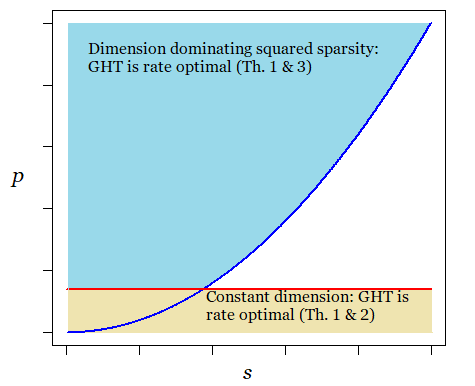
Figure 1: The rate optimality diagram in the minimax sense for the group hard thresholding estimator.

4 Concluding remarks and outlook

Combining the results of the previous sections one can draw the optimality diagram, see Fig. 1. In particular, 1 and Theorem 1 imply that the group hard thresholding estimator (6), (7) with the adaptively chosen threshold (8) is rate optimal when the term $sp$ dominates $s^{2}\sqrt{p}\,\log^{3/2}(2np)$. This corresponds to the “dimension dominates squared sparsity” regime $p\geq s^{2}\log^{3}(2np)$. According to 1 and Theorem 2, the estimator defined by (6), (7), (8) is rate optimal in the low dimensional setting $p=O(1)$ as well. The range of values of $p$ in which the determination of the minimax rate remains open corresponds to the regime $p\to\infty$ so that $p/s^{2}=O(1)$.

In a companion paper (Collier and Dalalyan, 2017), the problem of estimating the linear functional $\boldsymbol{L}(\mathbf{M})$ is considered, when the observations are Gaussian vectors with unknown means $\boldsymbol{\mu}_{i}$. It turns out that in the Gaussian setting the optimal scaling of the minimax risk is $ps+s^{2}$, up to a logarithmic factor. However, this rate is achieved by an estimator that has a computational complexity that scales exponentially with $n$. Furthermore, in the Gaussian model, the upper bound relies heavily on the fact that the Gaussian distribution is sub-Gaussian. The fact that the Poisson distribution is not sub-Gaussian (even though it is sub-exponential), does not allow us to apply the methodology developed in the Gaussian model.

It is worth mentioning here that although the risk bounds (both lower and upper) depend on the sparsity level $s$ and the largest intensity $\mu_{\infty}$, the group hard thresholding estimator is completely adaptive with respect to these parameters.

The problem we have considered in this work assumes that the noise variance $\sigma^{2}$ and the background signal $\boldsymbol{\mu}_{0}$ are known. It is not very difficult to check that the result of 1 can be extended to the case where $\boldsymbol{\mu}_{0}$ is unknown, but an additional data set $\bar{\boldsymbol{X}}_{1},\ldots,\bar{\boldsymbol{X}}_{m}$ is available, such that $\bar{\boldsymbol{X}}_{i}$’s are iid vectors drawn from the distribution $\sigma^{2}\mathcal{P}_{p}(\boldsymbol{\mu}_{0}/\sigma^{2})$. One can then estimate the background signal $\boldsymbol{\mu}_{0}$ by the empirical mean of $\bar{\boldsymbol{X}}_{i}$’s. As for $\sigma$, one can easily estimate this parameter using the fact that the entries of the data matrix $\mathbf{X}$ take their values in the set $\sigma^{2}\mathbb{N}$. Next, these estimates can be plugged in the group hard thresholding estimator. If $m$ is large enough, the error of estimating $\boldsymbol{\mu}_{0}$ and $\sigma^{2}$ is negligible with respect to the error of estimating $\boldsymbol{L}(\mathbf{M})$. Determining more precise risk bounds clarifying the impact of $m$ on the risk is an interesting avenue for future research.

5 Proofs of the lemmas

Proof of Lemma 1.

Let us introduce an auxiliary real number $\gamma>1.5^{2}$ and denote

$$Z_{j}=(\eta_{j}-\nu_{j}-0.5)^{2},\qquad Z_{j,\gamma}=Z_{j}\wedge\gamma,\qquad\bar{Z}_{j,\gamma}=(Z_{j}-\gamma)_{+}$$ (56)

as well as

$$\nu_{j,\gamma}=\mathbf{E}[Z_{j,\gamma}],\qquad\bar{\nu}_{j,\gamma}=\mathbf{E}[\bar{Z}_{j,\gamma}].$$ (57)

It is clear that $\nu_{j,\gamma}+\bar{\nu}_{j,\gamma}=\nu_{j}+0.25$ and we have

$$\|\boldsymbol{\eta}-\boldsymbol{\nu}\|_{2}^{2}-\|\boldsymbol{\eta}\|_{1} =\sum_{j\in[p]}(Z_{j,\gamma}-\nu_{j,\gamma})+\sum_{j\in[p]}(\bar{Z}_{j,\gamma}-\bar{\nu}_{j,\gamma})$$ (58)

$$=\|\boldsymbol{Z}_{\gamma}\|_{1}-\|\boldsymbol{\nu}_{\gamma}\|_{1}+\|\bar{\boldsymbol{Z}}_{\gamma}\|_{1}-\|\bar{\boldsymbol{\nu}}_{\gamma}\|_{1}.$$ (59)

Since the random variables $Z_{j,\gamma}$ are independent and bounded, with $\mathbf{P}(Z_{j,\gamma}\in[0,\gamma])=1$, the Hoeffding inequality yields

$$\mathbf{P}\Big{(}\|\boldsymbol{Z}_{\gamma}\|_{1}-\|\boldsymbol{\nu}_{\gamma}\|_{1}>t\Big{)}\leq e^{-2t^{2}/(p\gamma^{2})}.$$ (60)

On the other hand, it is clear that

$$\mathbf{P}\Big{(}\sum_{j\in[p]}\nolimits(\bar{Z}_{j,\gamma}-\bar{\nu}_{j,\gamma})>0\Big{)} \leq\mathbf{P}\big{(}\max_{j\in[p]}\nolimits Z_{j}>\gamma\big{)}$$ (61)

$$\leq p\/\max_{j\in[p]}\mathbf{P}\big{(}|\eta_{j}-\nu_{j}-0.5|>\sqrt{\gamma}\big{)}$$ (62)

$$\leq p\/\max_{j\in[p]}\mathbf{P}\big{(}|\eta_{j}-\nu_{j}|>\sqrt{\gamma}-0.5\big{)}$$ (63)

$$\leq p\/\max_{j\in[p]}\mathbf{P}\big{(}|\eta_{j}-\nu_{j}|>(2/3)\sqrt{\gamma}\big{)}.$$ (64)

Using the Bennet inequality for the Poisson random variables—see, for instance, (Pollard, 2015, Problem 15)— we get

$$\mathbf{P}\big{(}|\eta_{j}-\nu_{j}|>(2/3)\sqrt{\gamma}\big{)} \leq\mathbf{P}\big{(}\eta_{j}>\nu_{j}+(2/3)\sqrt{\gamma}\big{)}+\mathbf{P}\big{(}\eta_{j}<\nu_{j}-(2/3)\sqrt{\gamma}\big{)}$$ (65)

$$\leq e^{-1.54\gamma/(9\nu_{j})}+e^{-2\gamma/(9\nu_{j})}\leq 2e^{-\gamma/(6\nu_{j})},\qquad\forall\gamma\leq(9/4)\nu_{\infty}^{2}.$$ (66)

Combining (59), (60) and (66), we get

$$\mathbf{P}\Big{(}\|\boldsymbol{\eta}-\boldsymbol{\nu}\|_{2}^{2}-\|\boldsymbol{\eta}\|_{1}\geq t\Big{)}\leq\inf_{\gamma\in[(3/2)^{2},(9/4)\nu_{\infty}^{2}]}\Big{\{}e^{-2t^{2}/(p\gamma^{2})}+2pe^{-\gamma/(6\nu_{\infty})}\Big{\}}.$$ (67)

Let us set $t=\nu_{\infty}\sqrt{p}\,u$ and $\gamma^{3}=12\,u^{2}\nu_{\infty}^{3}$. For $u$ such that $\nu_{\infty}^{-3/2}\leq u\leq 0.9\nu_{\infty}^{3/2}$, the aforementioned value of $\gamma$ belongs to the range over which the infimum of the last display is computed. This yields

$$\mathbf{P}\Big{(}\|\boldsymbol{\eta}-\boldsymbol{\nu}\|_{2}^{2}-\|\boldsymbol{\eta}\|_{1}\geq\nu_{\infty}\sqrt{p}\,u\Big{)}\leq(2p+1)e^{-(12)^{1/3}u^{2/3}/6},$$ (68)

and the claim of the lemma follows. ∎

Proof of Lemma 2.

Using Markov’s inequality, we get

$$\sup_{\mathbf{M}\in\mathcal{M}}v^{-2}\mathbf{E}_{\mathbf{M}}\big{\|}\widehat{\boldsymbol{F}}-\boldsymbol{F}(\mathbf{M})\big{\|}_{2}^{2} \geq\sup_{\mathbf{M}\in\mathcal{M}}\mathbf{P}_{\mathbf{M}}\big{(}\|\widehat{\boldsymbol{F}}-\boldsymbol{F}(\mathbf{M})\|_{2}\geq v\big{)}$$ (69)

$$\geq\max_{i=0,1}\mathbf{P}_{\pi_{i}}\big{(}\|\widehat{\boldsymbol{F}}-\boldsymbol{F}(\mathbf{M})\|_{2}\geq v\big{)}-\max_{i=0,1}\pi_{i}(\mathcal{M}^{\complement}).$$ (70)

Now, using the test statistic $\psi=\arg\min_{i\in\{0,1\}}\big{\|}\widehat{\boldsymbol{F}}-\mathbf{E}_{\pi_{i}}(\boldsymbol{F})\big{\|}_{2}$ and the notation $M=\max_{i}\mathbf{Var}_{\pi_{i}}(F)=\max_{i}\mathbf{E}_{\pi_{i}}\|\boldsymbol{F}-\mathbf{E}_{\pi_{i}}[\boldsymbol{F}]\|_{2}^{2}$, we have

$$\mathbf{P}_{\pi_{i}}(\psi\neq i) =\mathbf{P}_{\pi_{i}}\Big{(}\big{\|}\widehat{\boldsymbol{F}}-\mathbf{E}_{\pi_{1-i}}(\boldsymbol{F})\big{\|}_{2}\leq\big{\|}\widehat{\boldsymbol{F}}-\mathbf{E}_{\pi_{i}}(\boldsymbol{F})\big{\|}_{2}\Big{)}$$ (71)

$$\leq\mathbf{P}_{\pi_{i}}\Big{(}\big{\|}\widehat{\boldsymbol{F}}-\mathbf{E}_{\pi_{i}}(\boldsymbol{F})\big{\|}_{2}\geq v+\sqrt{M/\alpha}\Big{)}.$$ (72)

Finally, using the triangle inequality again,

$$\mathbf{P}_{\pi_{i}}(\psi\neq i) \leq\mathbf{P}_{\pi_{i}}\Big{(}\|\widehat{\boldsymbol{F}}-\boldsymbol{F}(\mathbf{M})\|_{2}\geq v\Big{)}+\mathbf{P}_{\pi_{i}}\Big{(}\big{\|}\boldsymbol{F}(\mathbf{M})-\mathbf{E}_{\pi_{i}}(\boldsymbol{F})\big{\|}_{2}>\sqrt{\alpha^{-1}M}\Big{)}$$ (73)

$$\leq\alpha+\mathbf{P}_{\pi_{i}}\Big{(}\|\widehat{\boldsymbol{F}}-\boldsymbol{F}(\mathbf{M})\|_{2}\geq v\Big{)},$$ (74)

so that

$$\sup_{\mathbf{M}\in\mathcal{M}}\mathbf{P}_{\mathbf{M}}\big{(}\|\widehat{\boldsymbol{F}}-\boldsymbol{F}(\mathbf{M})\|_{2}\geq v\big{)}\geq\max_{i=0,1}\mathbf{P}_{\pi_{i}}(\psi\neq i)-\alpha-\max_{i=0,1}\pi_{i}(\mathcal{M}^{\complement}).$$ (75)

The result is now a direct application of Theorem 2.2 in Tsybakov (2009) using the assumption on the Kullback-Leibler divergence. ∎

Proof of Lemma 3.

Let us denote by $\mathbf{Q}_{\mu}$, for every vector $\mu\in(0,\infty)$, the Poisson distribution $\mathcal{P}(\sigma^{-2}\mu)$, and by $\mathbf{Q}_{\lambda}=\int_{(0,\infty)}\mathbf{Q}_{\mu}\,\lambda(d\mu)$, the $\lambda$-mixture of Poisson distributions. We have, for every $X\in\mathbb{N}$,

$$\frac{d\,\mathbf{Q}_{\lambda}}{d\,\mathbf{Q}_{\mu_{0}}}(X) =1+\frac{s}{2n}\Big{(}\frac{d\,\mathbf{Q}_{\mu_{0}+\sigma^{2}\epsilon}}{d\,\mathbf{Q}_{\mu_{0}}}(X)-1\Big{)}$$ (76)

$$=1+\frac{s}{2n}\Big{(}\Big{\{}1+\frac{\sigma^{2}\varepsilon}{\mu_{0}}\Big{\}}^{X}e^{-\varepsilon}-1\Big{)}.$$ (77)

Using the inequality $\log(1+t)\leq t$, we get

$${\rm KL}(\mathbf{Q}_{\lambda}\|\mathbf{Q}_{\mu_{0}})\leq\frac{s}{2n}\int_{\mathbb{N}}\Big{\{}1+\frac{\sigma^{2}\varepsilon}{\mu_{0}}\Big{\}}^{X}e^{-\varepsilon}\,\mathbf{Q}_{\lambda}(dX)-\frac{s}{2n}.$$ (78)

On the other hand, for every $\mu\in(0,\infty)^{p}$, we have

$$\int\Big{\{}1+\frac{\sigma^{2}\varepsilon}{\mu_{0}}\Big{\}}^{X}\,\mathbf{Q}_{\mu}(dX) =\sum_{k\in\mathbb{N}}\Big{\{}1+\frac{\sigma^{2}\varepsilon}{\mu_{0}}\Big{\}}^{k}\frac{\mu^{k}}{\sigma^{2k}k!}e^{-\mu/\sigma^{2}}=\exp\big{\{}\nicefrac{{\mu\varepsilon}}{{\mu_{0}}}\big{\}},$$ (79)

so that

$${\rm KL}(\mathbf{Q}_{\lambda}\|\mathbf{Q}_{\mu_{0}}) \leq\frac{s}{2n}\Big{(}1-\frac{s}{2n}\Big{)}+\Big{(}\frac{s^{2}}{4n^{2}}\Big{)}e^{\sigma^{2}\epsilon^{2}/\mu_{0}}-\frac{s}{2n}$$ (80)

$$=\frac{s^{2}}{4n^{2}}\big{(}e^{\sigma^{2}\varepsilon^{2}/\mu_{0}}-1\big{)}.$$ (81)

The result follows since, by independence, ${\rm KL}(\mathbf{P}_{\pi_{1}}\|\mathbf{P}_{\pi_{0}})=n{\rm KL}(\mathbf{Q}_{\lambda}\|\mathbf{Q}_{\mu_{0}})$. ∎

References

- Bickel and Ritov (1988) Bickel, P. J. and Ritov, Y. (1988). Estimating integrated squared density derivatives: Sharp best order of convergence estimates. Sankhyā: The Indian Journal of Statistics, Series A (1961-2002), 50(3):381–393.
- Birgé (2007) Birgé, L. (2007). Model selection for Poisson processes, volume Volume 55 of Lecture Notes–Monograph Series, pages 32–64. Institute of Mathematical Statistics, Beachwood, Ohio, USA.
- Boucheron et al. (2013) Boucheron, S., Lugosi, G., and Massart, P. (2013). Concentration Inequalities: A Nonasymptotic Theory of Independence. OUP Oxford.
- Brown et al. (2004) Brown, L. D., Carter, A. V., Low, M. G., and Zhang, C.-H. (2004). Equivalence theory for density estimation, poisson processes and gaussian white noise with drift. Ann. Statist., 32(5):2074–2097.
- Butucea and Comte (2009) Butucea, C. and Comte, F. (2009). Adaptive estimation of linear functionals in the convolution model and applications. Bernoulli, 15(1):69–98.
- Cai and Low (2004) Cai, T. T. and Low, M. G. (2004). Minimax estimation of linear functionals over nonconvex parameter spaces. Ann. Statist., 32(2):552–576.
- Cai and Low (2005) Cai, T. T. and Low, M. G. (2005). On adaptive estimation of linear functionals. Ann. Statist., 33(5):2311–2343.
- Cai and Low (2006) Cai, T. T. and Low, M. G. (2006). Optimal adaptive estimation of a quadratic functional. Ann. Statist., 34(5):2298–2325.
- Cai and Low (2011) Cai, T. T. and Low, M. G. (2011). Testing composite hypotheses, hermite polynomials and optimal estimation of a nonsmooth functional. Ann. Statist., 39(2):1012–1041.
- Collier et al. (2017) Collier, O., Comminges, L., and Tsybakov, A. B. (2017). Minimax estimation of linear and quadratic functionals on sparsity classes. Ann. Statist., 45(3):923–958.
- Collier et al. (2016) Collier, O., Comminges, L., Tsybakov, A. B., and Verzélen, N. (2016). Optimal adaptive estimation of linear functionals under sparsity. ArXiv e-prints, ArXiv:1611.09744.
- Collier and Dalalyan (2015) Collier, O. and Dalalyan, A. S. (2015). Curve registration by nonparametric goodness-of-fit testing. J. Statist. Plann. Inference, 162:20–42.
- Collier and Dalalyan (2017) Collier, O. and Dalalyan, A. S. (2017). Rate-optimal estimation of p-dimensional linear functionals in a sparse Gaussian model. ArXiv e-prints.
- Comminges and Dalalyan (2012) Comminges, L. and Dalalyan, A. S. (2012). Tight conditions for consistency of variable selection in the context of high dimensionality. Ann. Statist., 40(5):2667–2696.
- Comminges and Dalalyan (2013) Comminges, L. and Dalalyan, A. S. (2013). Minimax testing of a composite null hypothesis defined via a quadratic functional in the model of regression. Electron. J. Statist., 7:146–190.
- Donoho and Liu (1987) Donoho, D. and Liu, R. (1987). On Minimax Estimation of Linear Functionals. Technical report (University of California, Berkeley. Department of Statistics). Department of Statistics, University of California.
- Donoho and Nussbaum (1990) Donoho, D. L. and Nussbaum, M. (1990). Minimax quadratic estimation of a quadratic functional. Journal of Complexity, 6(3):290 – 323.
- Efromovich and Low (1994) Efromovich, S. and Low, M. G. (1994). Adaptive estimates of linear functionals. Probability Theory and Related Fields, 98(2):261–275.
- Golubev and Levit (2004) Golubev, Y. and Levit, B. (2004). An oracle approach to adaptive estimation of linear functionals in a gaussian model. Mathematical Methods of Statistics, 13(01):392–408.
- Grama and Nussbaum (1998) Grama, I. and Nussbaum, M. (1998). Asymptotic equivalence for nonparametric generalized linear models. Probability Theory and Related Fields, 111(2):167–214.
- Ingster and Kutoyants (2007) Ingster, Y. I. and Kutoyants, Y. A. (2007). Nonparametric hypothesis testing for intensity of the poisson process. Mathematical Methods of Statistics, 16(3):217–245.
- Ivanoff et al. (2016) Ivanoff, S., Picard, F., and Rivoirard, V. (2016). Adaptive lasso and group-lasso for functional poisson regression. Journal of Machine Learning Research, 17(55):1–46.
- Jia et al. (2013) Jia, J., Rohe, K., and Yu, B. (2013). The lasso under poisson-like heteroscedasticity. Statistica Sinica, 23(1):99–118.
- Juditsky and Nemirovski (2009) Juditsky, A. B. and Nemirovski, A. S. (2009). Nonparametric estimation by convex programming. Ann. Statist., 37(5A):2278–2300.
- Klemela and Tsybakov (2001) Klemela, J. and Tsybakov, A. B. (2001). Sharp adaptive estimation of linear functionals. Ann. Statist., 29(6):1567–1600.
- Koltchinskii (2011) Koltchinskii, V. (2011). Oracle inequalities in empirical risk minimization and sparse recovery problems, volume 2033 of Lecture Notes in Mathematics. Springer, Heidelberg. Lectures from the 38th Probability Summer School held in Saint-Flour, 2008,.
- Koshevnik and Levit (1977) Koshevnik, Y. A. and Levit, B. Y. (1977). On a non-parametric analogue of the information matrix. Theory of Probability & Its Applications, 21(4):738–753.
- Kutoyants (1998) Kutoyants, Y. (1998). Statistical Inference for Spatial Poisson Processes, volume 134 of Lecture Notes in Statistics. Springer New York.
- Kutoyants and Liese (1998) Kutoyants, Y. and Liese, F. (1998). Estimation of linear functionals of poisson processes. Statistics & Probability Letters, 40(1):43 – 55.
- Laurent et al. (2008) Laurent, B., Ludena, C., and Prieur, C. (2008). Adaptive estimation of linear functionals by model selection. Electron. J. Statist., 2:993–1020.
- Laurent and Massart (2000) Laurent, B. and Massart, P. (2000). Adaptive estimation of a quadratic functional by model selection. Ann. Statist., 28(5):1302–1338.
- Lepski et al. (1999) Lepski, O., Nemirovski, A., and Spokoiny, V. (1999). On estimation of the norm of a regression function. Probability Theory and Related Fields, 113(2):221–253.
- Pollard (2015) Pollard, D. (2015). A few good inequalities. Technical report, arXiv:1306.0187.
- Reynaud-Bouret and Rivoirard (2010) Reynaud-Bouret, P. and Rivoirard, V. (2010). Near optimal thresholding estimation of a poisson intensity on the real line. Electron. J. Statist., 4:172–238.
- Rudelson (1999) Rudelson, M. (1999). Random vectors in the isotropic position. Journal of Functional Analysis, 164(1):60 – 72.
- Shorack and Wellner (1986) Shorack, G. R. and Wellner, J. A. (1986). Empirical Processes with Applications to Statistics. Wiley, New York.
- Tsybakov (2009) Tsybakov, A. B. (2009). Introduction to Nonparametric Estimation. Springer Publishing Company, Incorporated, 1st edition.
- Verzelen and Gassiat (2016) Verzelen, N. and Gassiat, E. (2016). Adaptive estimation of High-Dimensional Signal-to-Noise Ratios. ArXiv e-prints.