Energy Calibration of CALET Onboard the International Space Station

Abstract

In August 2015, the CALorimetric Electron Telescope (CALET), designed for long exposure observations of high energy cosmic rays, docked with the International Space Station (ISS) and shortly thereafter began to collect data. CALET will measure the cosmic ray electron spectrum over the energy range of 1 GeV to 20 TeV with a very high resolution of 2% above 100 GeV, based on a dedicated instrument incorporating an exceptionally thick 30 radiation-length calorimeter with both total absorption and imaging (TASC and IMC) units. Each TASC readout channel must be carefully calibrated over the extremely wide dynamic range of CALET that spans six orders of magnitude in order to obtain a degree of calibration accuracy matching the resolution of energy measurements. These calibrations consist of calculating the conversion factors between ADC units and energy deposits, ensuring linearity over each gain range, and providing a seamless transition between neighboring gain ranges. This paper describes these calibration methods in detail, along with the resulting data and associated accuracies. The results presented in this paper show that a sufficient accuracy was achieved for the calibrations of each channel in order to obtain a suitable resolution over the entire dynamic range of the electron spectrum measurement.

1 Introduction

The CALET (CALorimetric Electron Telescope) [1] was docked to Exposed Facility of the Japanese Experiment Module (JEM-EF) on the International Space Station (ISS) in August 2015 and has been collecting data [2] since October 2015. It has been designed for long duration observations of high energy cosmic rays onboard the ISS. The CALET detector, shown in Fig. 1, includes a very thick calorimeter unit of 30 radiation-length ($X_{0}$), consisting of imaging and total absorption calorimeters (IMC and TASC, respectively).

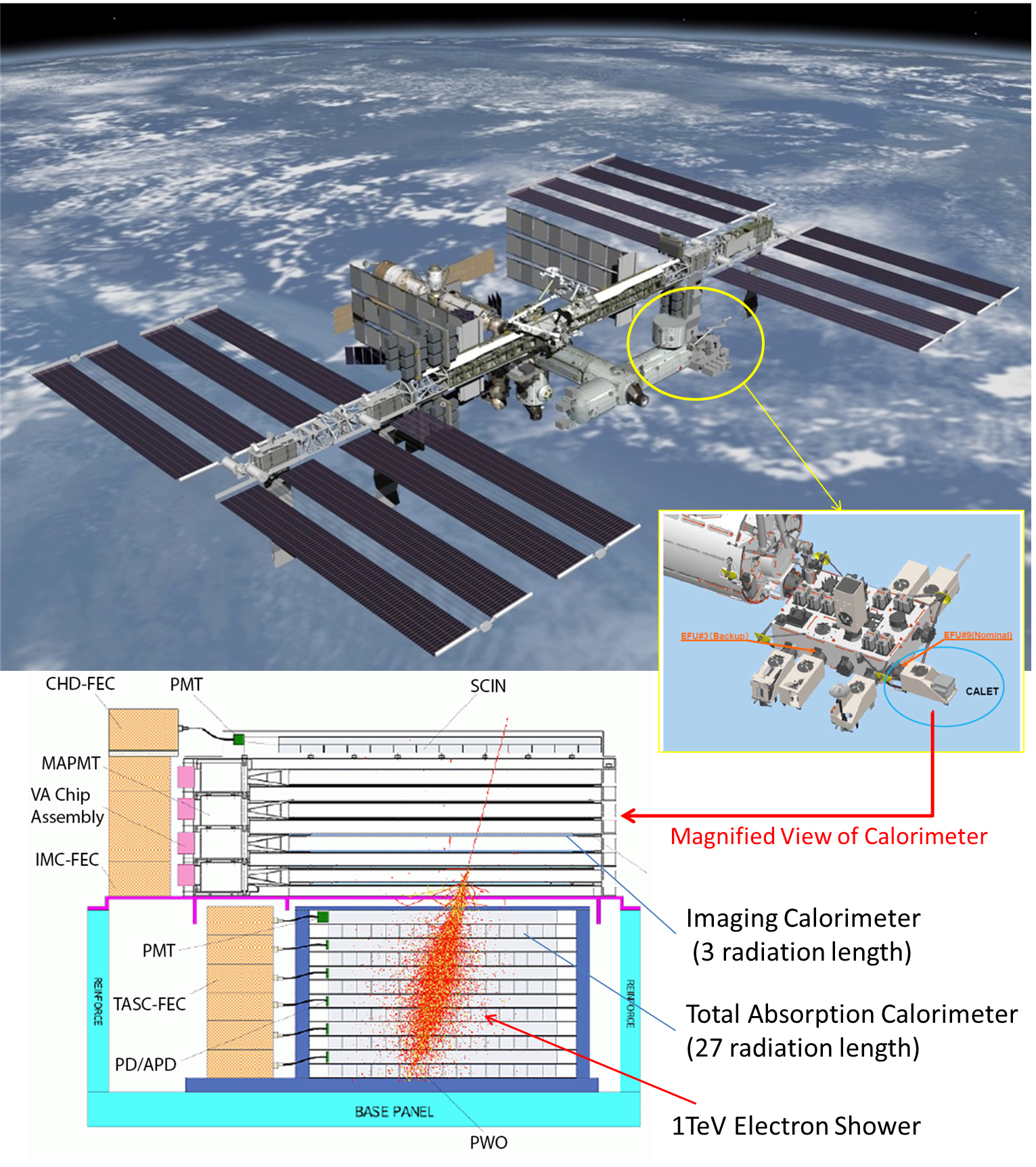
Figure 1: The CALET detector onboard the ISS as part of the Japanese Experiment Module - Exposed Facility [1].

.

The primary purpose of CALET is to make full use of a total-containment and well-segmented calorimeter to discover nearby cosmic-ray accelerators [3, 4] and to search for dark matter [5] with precision measurements of electron and gamma ray spectra over a wide energy range.

The calorimeter absorbs the majority of an electron shower’s energy in the TeV energy range and is able to identify electrons within a very high proton flux, with a rejection factor of $>10^{5}$, based on the difference in shower development. This instrument will therefore be used to acquire the cosmic ray electron spectrum over the energy range of 1 GeV to 20 TeV with exceptional energy resolution, especially above 100 GeV, where the resolution is better than 2%. Since each channel of the lead tungstate (PbWO₄) crystals of the TASC has a dynamic range of six order of magnitudes, CALET is capable of determining the energy of primary particles from 1 GeV to 1 PeV. This enables the instrument to measure proton and nuclei spectra as well as electron and gamma ray spectra over this extremely wide energy range.

The cosmic-ray detectors based on magnetic spectrometers that are presently in use (PAMELA [6] and AMS-02 [7]) have the significant advantage of being able to distinguish the sign of the charge on the particle. However, the spectral observations of these devices are limited to energy values below $\sim$1 TeV because their detector systems are optimized for the observation of various cosmic rays that have energies below this value. In addition, previous calorimeter-type instruments (ATIC [8] and Fermi-LAT [9]) were not optimized for the observation of electrons, and so at present their ability to identify electrons in the presence of a very high proton flux at higher energies is limited. In contrast, CALET is fully capable of measuring the electron plus positron spectrum well into the TeV region, as the result of being equipped with a thick 30 $X_{0}$ calorimeter. Due to its extremely high energy resolution and its ability to discriminate electrons from hadrons, CALET will allow the detailed search for various spectral structures of high-energy electron cosmic rays, perhaps providing the first experimental evidence of the presence of a nearby astrophysical cosmic-ray source. Even though it cannot distinguish the charge sign, CALET has the potential to detect distinctive features in the TeV region of electron plus positron energy spectrum possibly resulting from dark matter annihilation/decay. In the opposite scenario, the information acquired by CALET should make it possible to set significantly more stringent limits on dark matter annihilation compared to current experimental data [5].

There is an intrinsic advantage in measuring the electromagnetic components of cosmic rays with CALET. Since the TASC absorbs the majority of the energy ($\sim$95%) contained in an electromagnetic cascade, well into the TeV region, CALET is able to measure the primary energies of cosmic ray electrons and gamma rays with very small corrections. In principle, this should result in precise energy measurements with very low systematic errors. However, in order to achieve a calibration accuracy that matches the intrinsic energy resolution over the wide dynamic range of six orders of magnitude, a careful calibration of each TASC readout channel is required. The present paper details the calibration methods and results and also summarizes the accuracy of resulting energy measurements.

This paper is organized as follows. In Section 2, the CALET instrumentation is briefly summarized, while the energy measurements and calibration methods are described in Section 3. Section 4 presents each step of the CALET energy calibration process in detail, along with the resulting data. In Section 5, the calibration accuracy is studied and its effects on the energy resolution and absolute scale are assessed. Last, a summary and conclusions are presented in Section 6.

2 CALET Instrumentation

The CALET calorimeter, shown in side view in the lower part of Fig. 1 along with a simulation of a 1 TeV electron shower, has several unique and important characteristics, as briefly noted in the Introduction. These include its ability to resolve in detail the initial development of showers, as well as tracks generated by non-interacting minimum ionizing particles (MIPs), and its capacity to precisely measure the energy of electrons in the TeV region as a result of its depth of 30 $X_{0}$. These features are achieved through a combination of three primary detector sub-systems: Particle identification and energy measurements are performed by the TASC, charge identification is obtained from a charge detector (CHD), and an imaging calorimeter (IMC) is employed for track reconstruction. The key performance of each detector component, as described below, was estimated on the basis of a detailed Monte Carlo (MC) simulation and was confirmed by several beam tests carried out primarily at the CERN-SPS facility.

Plastic scintillators arranged in two orthogonal layers, each containing 14 scintillator paddles (3.2 $\times$ 1.0 $\times$ 44.8 cm³), constitute the CHD. These paddles generate photons that are detected by a photomultiplier tube (PMT), and the resulting output is sent to a front end circuit (FEC). This FEC and the subsequent readout system have sufficient dynamic range for particle charges in the range of $Z=1\sim 40$. The charge resolution of the CHD spans the range from 0.15 electron charge units ($e$) for boron to $\simeq 0.30-0.35e$ in the iron region [10].

The initial shower is visualized by the IMC sampling calorimeter, which has been carefully designed to accurately determine the shower starting point and incident direction. This calorimeter has a thickness of 3 $X_{0}$ and contains five upper 0.2 $X_{0}$ and two lower 1.0 $X_{0}$ tungsten plates. The IMC contains a total of 16 detection layers, arranged in 8 X-Y pairs, with each layer segmented into 448 parallel scintillating fibers (0.1 $\times$ 0.1 $\times$ 44.8 cm³), which are read out by 64-channel multi anode PMTs. By reconstructing the trajectory of incident particles in the IMC, the arrival direction of each individual particle can be determined. Above several tens of GeV, the expected angular resolution for gamma-rays is $\sim 0.24^{\circ}$, while the angular resolution for electrons is better and close to $\sim 0.16^{\circ}$ [1].

The TASC has an overall depth of 27 $X_{0}$ and consists of 12 detection layers in an alternating orthogonal arrangement, each comprised of 16 lead tungstate crystal (PbWO₄ or PWO) logs with dimensions of 2.0 $\times$ 1.9 $\times$ 32.6 cm³. As a result of this design, the TASC is able to image the development of the shower in three dimensions. With the exception of the first layer which uses PMTs, a photodiode (PD) in conjunction with an avalanche photodiode (APD) reads the photons generated by each PWO log. Employing dual shaping amplifiers with two different gains for each APD (PMT) and PD, increases the dynamical range to 10⁶ (10⁴). As a consequence, the TASC can measure the energy of the incident electrons and gamma rays with a resolution $<2$% above 100 GeV [11]. Another important role of the TASC is to efficiently identify high-energy electrons among the overwhelming background of cosmic-ray protons. Particle identification information from both the IMC and TASC is used to achieve an electron detection efficiency above 80 % and a proton rejection power of $\sim 10^{5}$ [12].

A preselected combination of simultaneous trigger counter signals, which are produced by discriminating the analog signals from the detector components, generates an event-trigger decision. As such, each of CHD X and Y, IMC X1–X4, Y1–Y4 and TASC X1 generates lower discriminator signals [2]. The signals from two IMC fiber layers are processed by a single front end circuit, and so each axis has only four trigger counter signals. Three trigger modes are possible in CALET. The High Energy (Low Energy) Trigger select shower events with energies greater than 10 GeV (1 GeV), while the Single Trigger is dedicated to acquiring data from non-interacting particles for the purposes of detector calibration.

3 Energy Measurement and Calibration Method

As briefly introduced in Section 1, careful calibration of each TASC readout channel is required in order to achieve a calibration accuracy that matches the intrinsic energy resolution over the wide dynamic range of six orders of magnitude. The entire dynamic range is covered by four different gain ranges, based on two photon detectors - an APD and a PD - in conjunction with a shaper amplifier with lower and higher gains. The energy calibration process consists of three steps as follows:

1. determination of the conversion factor between ADC units and the energy deposit,

2. linearity measurements over each gain range,

3. correlation measurements between adjacent gain ranges.

The first step is the calibration of the energy deposit of each channel to obtain an ADC unit-to-energy conversion factor using MIPs, known as MIP calibration. As it is the case with other detectors intended for direct cosmic-ray measurements, CALET can use penetrating particles to equalize the gains of different detector segments, based on the fact that the energy deposits of such particles in the relativistic energy range are approximately constant. In contrast with the calibration of a spectrometer, MIP calibration serves as an absolute energy calibration of the CALET because this instrument is a total absorption calorimeter. Therefore, absolute end-to-end energy calibrations are possible using the MIP technique. End-to-end calibration stands for the summary treatment of all detector responses transforming the particle’s energy loss to the output signal, such as PWO scintillation yield, photon propagation in the PWO, quantum efficiency of the APD/PD, gain of the front end circuit and others.

Prior to launch, the linearity over each gain range was confirmed by on-ground calibration using a UV pulse laser, during which the APD and PD outputs were determined as a function of the laser energy. In this process, the UV laser pulse was absorbed by the PWO, while the APD and PD detected the resulting scintillation emissions resulting from de-excitation of the PWO. By scanning the UV laser pulses over the entire energy range, it was therefore possible to calibrate the input-to-output correspondence for all four gain ranges.

The adjacent gain ranges were subsequently cross-calibrated based on their gain ratios. Taking advantage of the nearly one order of magnitude overlap between adjacent gain ranges, it was possible to measure identical energy deposits within two gain ranges. In contrast to the MIP calibration process, which requires a dedicated trigger mode, for gain correlation measurements all the data regardless of trigger modes can be used. This is helpful especially for PD range correlation measurements because such measurements require a long term accumulation of data for very high energy events. As the linearity of each gain range had already been confirmed, the gain over entire dynamic range could be determined based on the ADC-to-energy conversion factor, using the acquired gain ratios between adjacent gain ranges. This process automatically takes into account possible gain changes due to the flight environment. Such gain changes are expected to occur due to variations in temperature between flight and ground calibration. Special care was also required to account separately for the effects of the flight environment on the APD gain and the light yield of the PWO, which in turn affects both the APD and PD gain ranges.

4 Energy Calibration

4.1 MIP Calibration

It is an important advantage of the CALET instrument that an absolute end-to-end calibration of the energy scale is possible, by employing the MIP technique. While 10% accuracy is relatively easy to achieve using MIPs, more accurate calibration requires careful analysis of the energy distribution of incident particles, appropriate penetrating particle event selection, and consideration of the position and temperature dependence of each TASC log. The latter is especially important because CALET employs a one-end readout system and because of the relatively high temperature dependence of both the PWO and APD. This aspect of the calibration process is discussed in detail in the following section.

While the energy deposits of relativistic particles are approximately constant and close to minimum ionization, the sample used for MIP calibration also includes particles outside the minimum ionizing region. Their energy spectrum depends on the cutoff rigidity, and hence the geomagnetic latitude. As a result, the position of the MIP peaks will shift by several percent as a function of the geomagnetic latitude [11]. To account for this effect, the incident particle energy distributions are assessed by simulating the energy spectra of incoming primary particles [11] using ATMNC3 [13], in which AMS-01 proton and helium spectra [14] were used as input, since these data were taken at various geomagnetic latitudes, as well as them being in good agreement with BESS [15] and recent experiments. As well, contamination by interacting particles and/or scattered and stopped particles can cause a systematic shift in the determined position of MIP peaks. In order to avoid this, the appropriate selection of penetrating particle events is ensured using a likelihood analysis [11]. To further improve the selection efficiency and to reduce systematic bias during event selection, the likelihood ratios of penetrating particles to interacting particles are also employed. By taking the ratios, the separation of penetrating particles from interacting particles becomes better, while possibly remaining discrepancies between flight and MC data have less influence.

Event selection based on likelihood uses energy deposit distributions obtained from an MC simulation including the detector response of each channel. Simulating this detector response requires data regarding the noise levels in units of energy, which in turn requires the ADC unit-to-energy conversion factor. Because this conversion factor is obtained from the calibration, the MIP calibration is performed as an iterative procedure. However, this process converges very quickly and a single iteration is sufficient to obtain stable results when calibrating CALET.

4.1.1 Position and Temperature Dependence Corrections

To fully calibrate each TASC log, it is first necessary to correct for the position dependent effects so as to equalize the response along its length. In addition, because both the PWO light yield and the APD gain will vary with temperature, it is also required to correct for this temperature dependence. During the calibration process, the temperatures inside the TASC were calculated from temperature data measured during flight using a software that parameterized the temperature distribution in the TASC based on the CALET thermal model. The CALET flight model is equipped with 14 thermocouples located around the TASC structure. The CALET thermal model was calibrated using the flight instrumentation results obtained from a thermal vacuum test performed at the JAXA Tsukuba Space Center. Figure 2 presents the average temperature distributions inside the X1 (Top) and Y6 (Bottom) layers of the TASC. Here, the left side panels show the two-dimensional temperature distributions, while the right side panels show the positional temperature dependence along the length of each unit. Since it is not possible to differentiate between the gain change due to the general temperature slope and the inherent position dependence, the position dependence correction includes both effects.

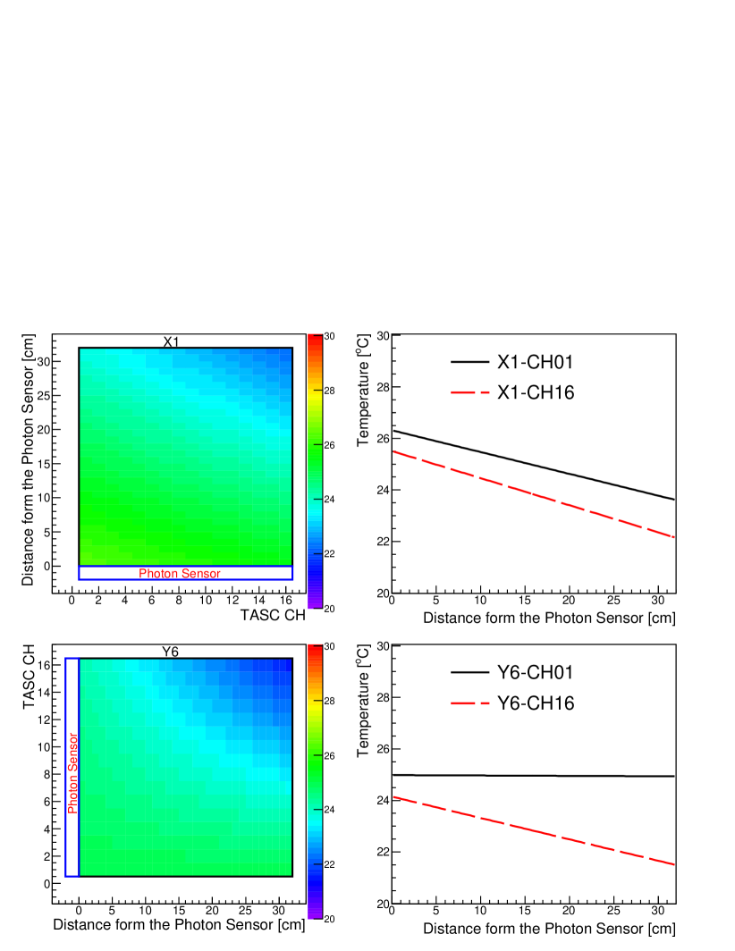
Figure 2: Temperature distributions in the TASC X1 (Top Left) and Y6 (Bottom Left) units, averaged over four months. Right side panels show the positional temperature variations along the length of each unit. The black solid and red dashed lines in the Top Right (Bottom Right) panels represent X1-CH01 and X1-CH16 (Y6-CH01 and Y6-CH16) data, respectively.

These data clearly show that the temperature tends to decrease along the length of each unit.

To correct for this position dependence, MIP peaks were determined for each of 16 segments defined along the length of each TASC log. Subsequently, the position dependence of these MIP peaks for each log was fitted using an appropriate function of distance from the sensor (the PMT or APD/PD). To ensure that the correct positional dependence was derived in each case, several different functions were defined. Figure 3 presents an example of the position dependence of a MIP peak both before and after the correction process.

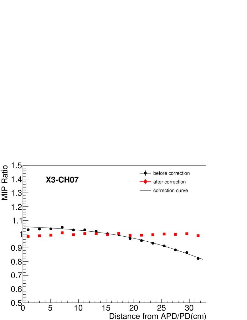
Figure 3: An example of the position dependence of the MIP peak for a typical TASC log. The filled black and red circles represent data before and after the correction, respectively. The black line indicates the function used to fit the position dependence.

On average, a position dependence of 9.2% RMS was observed for a total of 192 PWO logs, and these data were successfully corrected. Following this correction, the RMS of the position dependence was reduced to 1.8%.

In addition to the general temperature slopes in the TASC logs, there was also an overall temperature variation due to the dependence of temperature related to both the solar beta angle and the solar altitude. To discriminate between these temperature variations and the position dependence due to temperature gradients in the TASC log data, we have obtained the averaged temperature at the center of each log and averaged temperature gradient to calculate a position dependent reference temperature for each track. The correction for temperature dependence then employed the difference from the reference temperature. In this manner, the data were corrected for both the beta angle dependence and the overall temperature changes due to solar altitude without interfering with the position dependence correction. Figure  4 presents examples of the overall temperature dependence of MIP peaks over a period of seven months, together with solar beta angle variations over time (in the upper graph) and temperature variations for both the TASC X1 and Y6 layers.

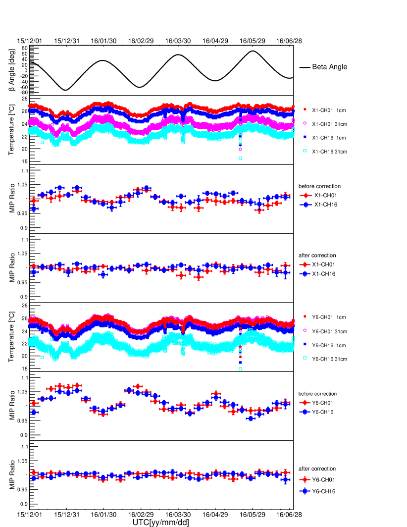
Figure 4: The relationship between the beta angle, temperature and MIP peaks. The upper graph plots the time variation of the beta angle. The second graph shows the variations over time of the temperatures of four segments located in the corners of TASC X1. The third and fourth graphs represent the MIP variations of two different channels at both ends of TASC X1, before and after the temperature dependence correction. The last three graphs represent the same type of data for TASC Y6.

These data indicate that the MIP peak variation rate due to the temperature changes was, on average, -1.9% per degree for the PMT channels, and -3.4% for the channels with an APD. Since these observed temperature dependences of the MIP peaks were consistent with one another within the associated errors, the average values for the PMT and APD were adopted as universal gain corrections independent of the PWO logs and reference temperatures. Thanks to the performance of the active thermal control system (ATCS) available in the JEM-EF, temporal variations in the temperature were typically within a few degrees. On average, a temperature dependence of 3.3% RMS was observed for 192 PWO logs, and this variation was successfully corrected for, reducing the RMS variation to 1.0%.

4.1.2 Determination of the Energy Conversion Factor

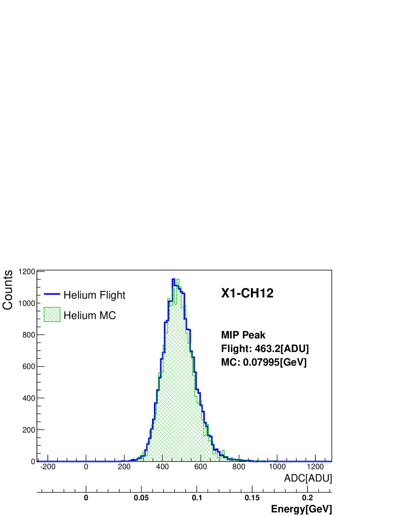
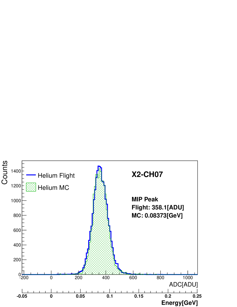
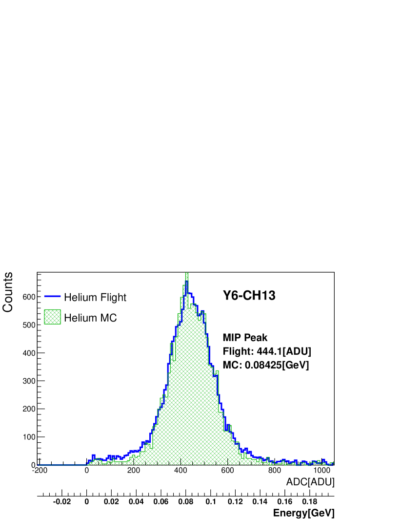
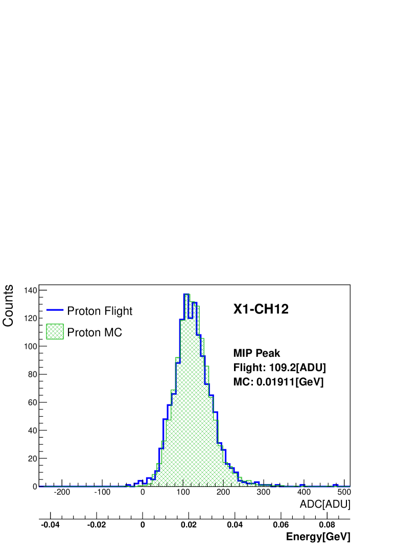
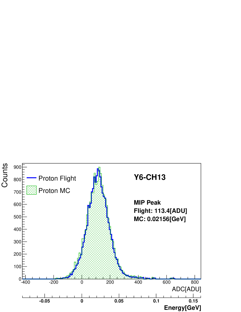
Figure 5: Comparisons of distributions of flight and simulated helium and proton data. Blue open and green hatched histograms represent flight and MC data, respectively. The top three plots provide helium distributions, while the bottom three show proton distributions. Data from one PMT channel (Left), one typical APD/PD channel (Middle) and one APD/PD channel in the bottom layer (Right) are shown.

Following the corrections for the position and temperature dependence described in Section 4.1.1, accurate calculations of the MIP peaks in ADC units (ADU) could be obtained from the flight data, while MIP peaks in energy units could be determined from the simulated MC data. Subsequently, with the MIP peak values in both ADU and GeV, it was possible to find the energy conversion factor, GeV/ADU. In order to verify the accuracy of this conversion factor, factors were calculated for both proton and helium data. As shown in Fig. 5, clear peaks resulting from penetrating helium (Top) and protons (Bottom) were extracted using event selection based on likelihood analysis for both flight and MC event data. The MC event data were generated from a CALET detector simulation [12] with the detector simulation tool EPICS [16] using the ATMNC3 results as input data. The energy deposit of EPICS for PWO was confirmed to be consistent within 1% with the beam test data and with the Geant4 results [17]. In Fig. 5, data from one PMT channel (Left), one typical APD/PD channel (Middle) and one APD/PD channel in the bottom layer (Right) are shown. The conversion factor was calculated by comparing MIP distributions between flight and MC data; each distribution was fitted with an appropriate function and the ratio of the peaks gave the conversion factor. It is very important to properly smear the MC distribution according to the relevant noise factors. To do so, the Gaussian sigma of the fitted pedestal distribution of each TASC channel was used to incorporate electronic noise into the simulation. Fluctuations due to photoelectron statistics were included especially in the case of the TASC X1 channels equipped with PMTs, in addition to the pedestal noise, because such fluctuations have a significant effect due to the lower level of pedestal noise in these channels compared to APD channels. The accuracy of each conversion factor was estimated from the errors in the peak fits on a channel-by-channel basis. On average, the accuracy values were 1.6% and 0.6% for protons and helium, respectively. To ensure robustness of fit results, the fit range dependence of peak value was also investigated by changing the fit range by $\pm$33% from its optimal value and it was found that such dependencies were reasonably small as 0.4% and 0.6% for protons and helium, respectively. They are included in both calibration error and systematic uncertainty on the energy scale. Since the helium data have better statistics and a superior signal-to-noise ratio, it is evident that the more accurate determination of conversion factors was achieved using the helium data.

Although this paper is focused on the calibration of the TASC, the same method is applicable to the CHD and IMC, and in fact was employed when equalizing and calibrating the energy deposit of each of their channels.

4.1.3 Estimation of Calibration Accuracy

While it is relatively easy to estimate the accuracy of the calculated position and temperature dependences because it is possible to check the equalizations after applying the corrections, it is generally more difficult to evaluate the accuracy of the absolute calibration. One key test to confirm the validity of the absolute calibration of the energy conversion factor is to assess the consistency between proton and helium data. This is because the A/Z difference between protons and helium results in different primary energy distributions at equivalent rigidity cutoffs and also because the different signal-to-noise ratio will affect the event selection of penetrating particles should there be any such dependences. As shown in Fig.6, excellent agreement was obtained between conversion factors obtained from proton and helium MIP data. This figure plots the conversion factors obtained in the case of proton MIPs divided by those generated from helium MIP data for all TASC logs. From the resulting distribution, it is concluded that, on average, the conversion factors agree within 0.1%, and the observed deviations from unity are slightly larger than the combined errors in the conversion factors including the uncertainty from the energy distribution of the used events, which is studied in the following. To account for this small inconsistency, an additional calibration error of 1.0% is allocated as a systematic uncertainty.

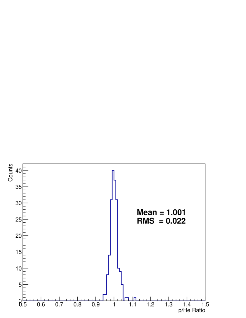
Figure 6: Comparison of conversion factors obtained from proton and helium MIPs. The histogram represents the distribution of the proton MIP conversion factors divided by those obtained from helium MIPs for each TASC log.

To directly evaluate the effects of the energy distribution of incoming particles, the MIP peak variations due to the rigidity cutoff were compared between the helium flight and MC data. Both data displayed similar trends, although there were small discrepancies at the low cutoff region, where low energy particles play an important role. This could result from inaccuracy of the solar modulation parameter or insufficient MC statistics. Herein, a conservative estimate of a potential discrepancy of 1.0% is introduced for the systematic uncertainty in the energy scale and in the calibration accuracy.

4.2 Linearity Measurements over the Entire Dynamic Range

It was necessary to determine the input-output relationship over each gain range with ground-based measurements prior to launch because such measurements are no longer possible in orbit. However, the relative gain change between the four ranges can be monitored and corrected using gain ratio measurements, as explained in the following section. UV pulse laser calibrations were performed on ground for linearity confirmation. While scanning the pulse laser intensity through six orders of magnitude, detailed measurements were made of the four APD/PD output responses from each of the 176 PWO logs. Figure 7 provides a schematic diagram of the UV pulse laser injection into the PWO, from the opposite end to the APD/PD. Since the UV photons are absorbed within a very short distance, all the photons seen by the APD/PD are the result of PWO scintillation, which has a very similar spectrum as that generated by charged particles. Figure 7 also shows the hybrid APD/PD package and subsequent readout system. By combining four readouts, the full dynamic range of six orders of magnitude is covered while maintaining a nearly one order of magnitude overlap between adjacent gain ranges. It should be noted that there is crosstalk from the APD to the PD due to stray capacitance between these two devices. When the charge sensitive amplifier (CSA) of the APD is saturated, the feedback from the CSA becomes insufficient and the potential at the APD-CSA input has a non-zero value, which induce a signal in the PD. Although the crosstalk amounts to only $\sim$0.1% of the charge ratio, it can become significant due to the APD-PD gain/area ratio of 1000 to 1 (APDs have a 20 times larger area and a 50 times higher gain). Since the crosstalk signal is proportional to the input charge and is stable, it is possible to calibrate the input-output relationship using UV pulse laser data.

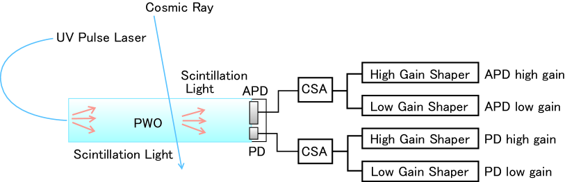
Figure 7: Schematic view of UV pulse laser light injection into the PWO, together with TASC APD/PD readouts.

Figure 8 shows an example of the data obtained from UV pulse laser measurements. Here, the horizontal and vertical axes represent the laser energy and ADC values, respectively. Since the laser energy is monitored on a pulse-by-pulse basis, the linearity over the entire dynamic range was confirmed using 17,000 points of laser pulse data for each channel. As a result of the APD/PD crosstalk, the PD response exhibits a slope break corresponding to the APD-CSA saturation point, as shown in the right panel of Fig. 8. The responses of all APD/PD channels were measured and the data confirmed the linear and broken linear relationships of the APD and PD response functions, respectively, as a result of fitting of the data points with appropriate functions for each range.

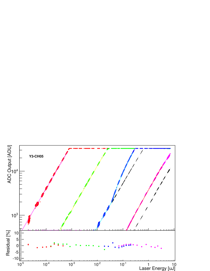
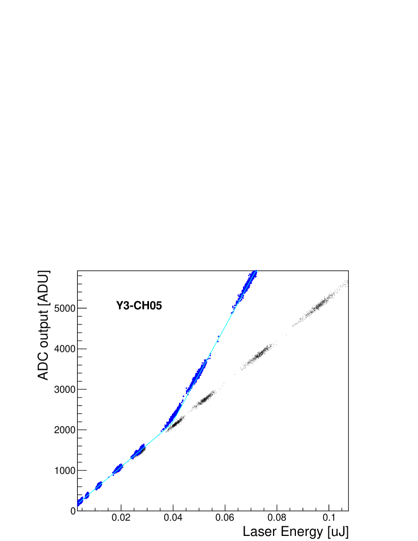
Figure 8: Typical data acquired from UV pulse laser calibration. (Left) From left to right, the responses of the APD high gain (red data points), APD low gain (green), PD high gain (blue) and PD low gain (magenta) are plotted as a function of laser energy with the residuals from fitted functions shown in the bottom panel. Black points in the PD range represent data acquired without an APD bias. (Right) Close up view of the PD high gain response, applying a linear scale to better demonstrate the simple broken linear relationship.

To estimate the errors resulting from fitting the linear and broken linear functions, the distributions of residuals from the fitting functions were assessed for each gain range. From the RMS of each distribution, the errors were estimated to be 1.4%, 1.5%, 2.5% and 2.2% for the APD high gain, APD low gain, PD high gain and PD low gain, respectively. Although these errors include both possible nonlinearities and expected statistical variations in measurements, in addition to UV laser system calibration errors, we adopted these values as the actual errors due to possible non-linear effects.

It is expected that both the APD gain and the PWO light yield will vary between on-ground conditions and those onboard the ISS, as well as with time during on-orbit observations. This corresponds to a change in the amount of crosstalk charge per unit energy deposit and thus results in a slope change in the APD/PD crosstalk region. We confirmed this effect using UV laser data acquired at a higher APD bias ($\sim\times$2 gain). During this laser calibration process, three data sets with different APD gains (nominal gain, $\sim\times$2 gain and small gain without APD bias) were obtained to validate our simple model for correcting APD/PD crosstalk and to estimate the correction errors, as well as to calibrate all the gain ranges. This effect is revisited in the next section in relation to gain correlation measurements.

4.3 Cross Calibration of Adjacent Gain Ranges

The gain correlations between adjacent gain ranges were used to correct for possible gain changes between the UV laser calibrations performed on the ground and observations onboard the ISS. Figure 9 presents examples of gain ratio measurements in the APD high gain to APD low gain (Left), APD low gain to PD high gain (Middle), and PD high gain to PD low gain (Right) regions.

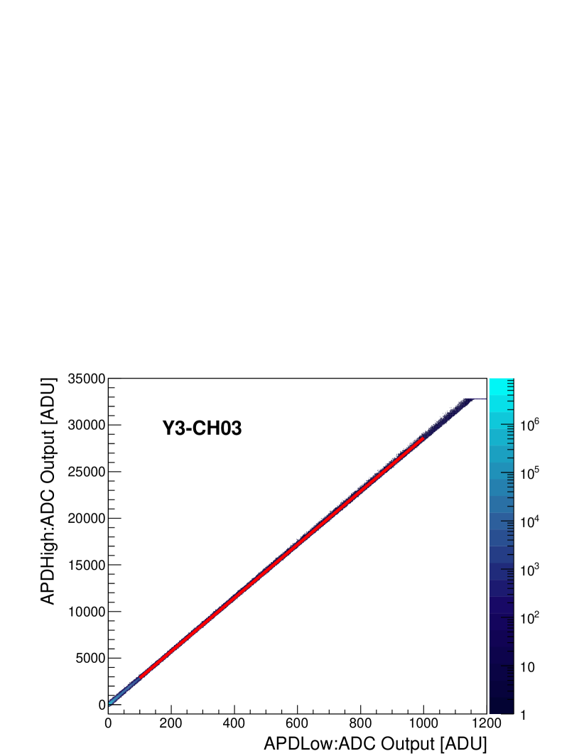
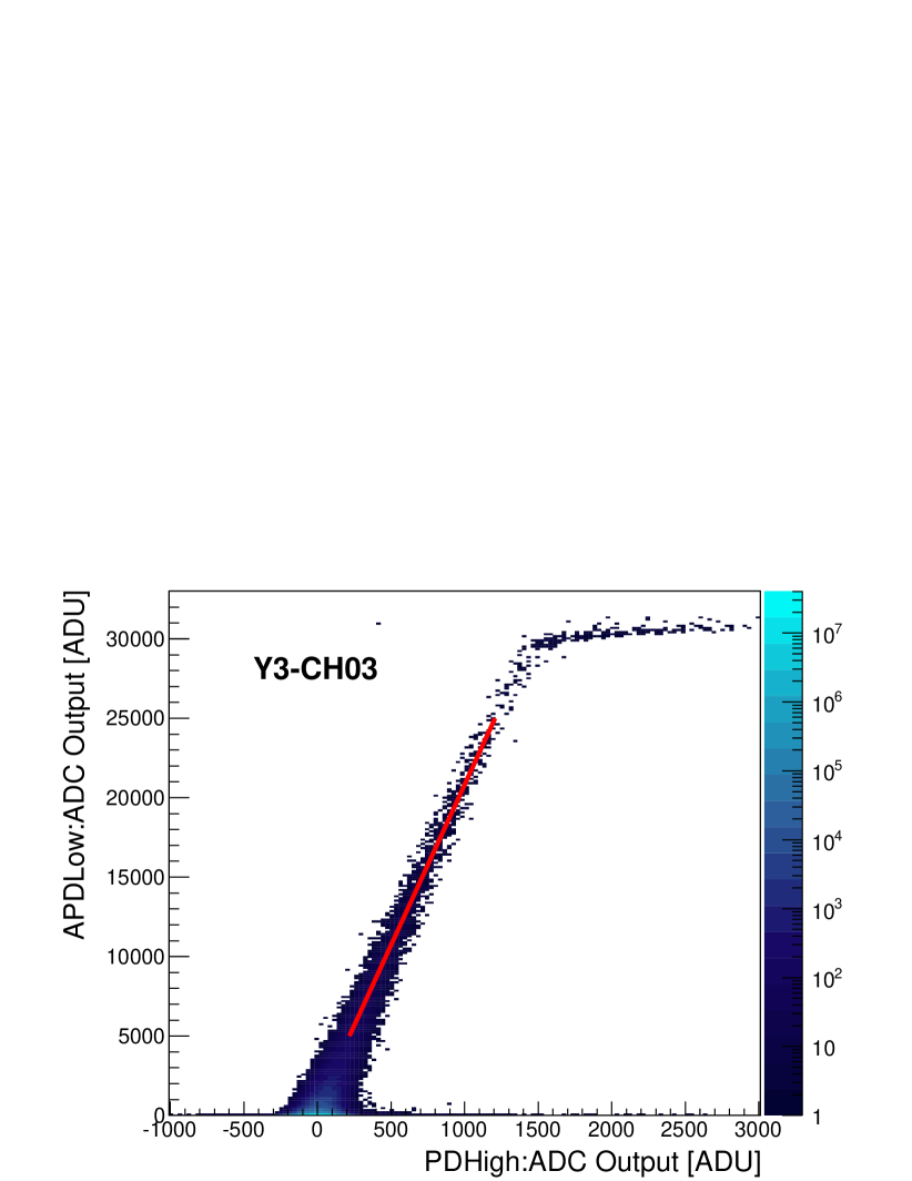
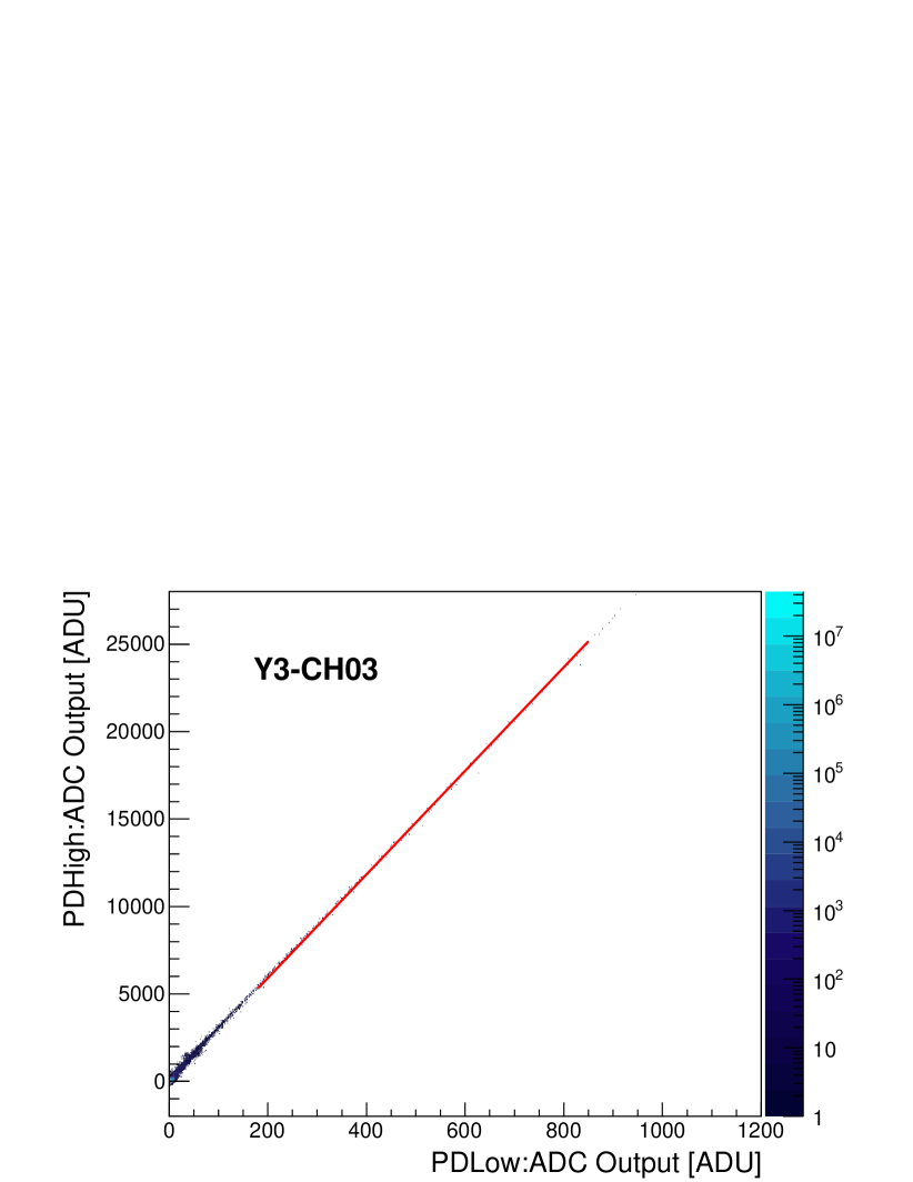
Figure 9: Typical gain correlation from flight data between adjacent gain ranges. (Left) APD high gain to APD low gain, (Middle) APD low gain to PD high gain, and (Right) PD high gain to PD low gain regions.

Taking advantage of the nearly one order of magnitude overlap between adjacent gain ranges, the same energy deposit was measured with two gain ranges and the gain ratio required to connect the two gain ranges was determined by fitting the profile with a simple linear function. In the fitting of each channel, proper selection of the fitting range was vital in order to avoid saturation effects in the higher gain range and the lower signal-to-noise region due to pedestal noise in the lower gain range. While the offset was set to zero in most cases, non-zero offsets during linear fitting were allowed in some caces involving PD-high to APD-low gain ratio fitting due to APD-to-PD crosstalk prior to APD-CSA saturation. In such cases, correct treatment was ensured by using the same offset during linear fitting of the UV pulse laser data. The errors on the gain ratios were determined from the parameter errors in the linear fittings since the reduced chi-squared distributions were found to be reasonable, having average values of approximately 1. The errors on the ratios were found to be 0.1%, 0.7% and 0.1% for the APD high gain to APD low gain, PD high gain to APD low gain and PD high gain to PD low gain regions, respectively.

As explained in the previous section, slope changes in the on-orbit calibration of the APD range with respect to the ground data were foreseen due to the different environment experienced in orbit. This also affects the APD-to-PD crosstalk region, which was corrected based on the assumption that the slope change in the PD range after APD-CSA saturation is proportional to the slope change in the APD range between ground and orbit. When applying such corrections, it is important to identify the crosstalk component because the slope associated with the PD gain is not affected by the APD gain change. UV laser data acquired with a $\sim\times$2 gain were used to validate the correction method and to estimate the associated errors. By applying the same procedure to $\sim\times$2 gain data and comparing the predicted slope with the measured slope in the PD high gain range above APD-CSA saturation point, we were able to estimate the errors associated with our simple model for the correction of the APD-PD crosstalk effect. When applying this method to on-orbit data, the error was scaled to the actual in-flight gain difference of $\sim$10%, and the resultant error on the gain was estimated to be 1.1%. Since it is not possible to determine this error from the on-orbit data, we consider this error to represent a systematic uncertainty on the energy scale as well as an estimation of the calibration error that affects the energy resolution.

Since the UV laser tests confirmed the linearity of each gain range, calibration over the entire dynamic range is now possible by applying the conversion factor to the subsequent gain range using the gain ratios. Figure 10 shows a typical calibrated energy deposit spectrum for one TASC channel. A smooth transition between adjacent gain ranges is clearly observed.

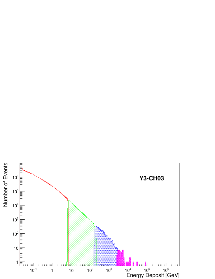
Figure 10: A typical energy deposit spectrum after applying full calibration. Open red, hatched green, dotted blue and filled magenta histograms correspond to APD high, APD low, PD high and PD low gain ranges, respectively.

To determine the errors due to extrapolation from the region in which the gain ratio was measured to the uppermost point in each gain range, the slopes were compared between the gain ratio region and the full range for each gain range by employing UV laser data. Using the RMS of the distribution of the relative slope changes obtained from all the TASC channels, the errors were estimated as 1.6% and 1.8% for the APD high gain to APD low gain and PD high gain to PD low gain regions, respectively. Note that the RMS is dominated by the UV laser test statistics which is limited especially in the overlapping region due to shorter lever arm. Since there is no systematic shift in their slopes, these extrapolation errors can be considered as a part of the calibration accuracy, rather than a component of the energy scale uncertainty. The APD low gain to PD high gain extrapolation error was estimated at a higher value 2.0%, to account for possible gain changes relative to the on-ground calibration. This conservative error estimate should be considered as a component of the energy scale uncertainty.

5 Energy Measurement: Error and Resolution

Table 1 summarizes the error budget for CALET energy measurements based on the discussions in the previous sections. Note that the systematic error in the energy measurements resulting from the MC simulation based on EPICS is negligible below the energy of 95% containment for electromagnetic showers ($\sim$20 TeV). Highly detailed detector geometries and materials were employed in our MC simulation, based on the CAD model for the CALET detector.

Table 1: Summary of the error budget in the energy calibration.

MIP		Energy conversion	2.6%
Peak fitting of MC and flight data			0.6%
Fitting range dependence			0.6%(∗)
Position dependence			1.8%
Temperature dependence			1.0%
Rigidity cutoff dependence			1.0%(∗)
Systematic uncertainty estimated
from p/He consistency			1.0%
UV Laser		Linearity	1.4$\sim$2.5%
Fit error
APD high gain			1.4%
APD low gain			1.5%
PD high gain			2.5%
PD low gain			2.2%
Gain Ratio		Gain range connection	1.6$\sim$2.1%
Fit error
APD-high to APD-low gain			0.1%
APD-low to PD-high gain			0.7%
PD high to PD low gain			0.1%
Slope extrapolation
APD-high to APD-low gain			1.6%
APD-low to PD-high gain			2.0%(∗)
PD high to PD low gain			1.8%
Sampling Bias			0.5%(∗∗)
(∗) also considered as systematic error on energy scale
(∗∗) energy-scale systematic error only

Using the estimated calibration errors and measured detector responses, such as the pedestal noise on a channel-by-channel basis, the errors in the energy deposit sum were calculated for simulated electron events from 1 GeV to 20 TeV. The top panel of Fig. 11 presents the energy dependence of the relative error in the energy deposit sum measurements. As clearly shown by this figure, a 2% precision level energy calibration was achieved over the entire dynamic range above 10 GeV. The reduced accuracy with which the energy deposit can be determined below 10 GeV is due to pedestal noise. As reported in detail in Ref. [11], the requirements for the calibration error of each TASC log can be relaxed by a factor of $\sim$3 compared to that for the energy resolution, as long as these individual errors of in total $\sim$6% are randomly distributed. This is due to the fact that, on average, $\sim$10 TASC logs contribute significantly to an event’s energy measurement. The results obtained here are therefore perfectly consistent with the expected values.

The estimated systematic uncertainty is also plotted on an absolute scale in Fig. 11. The systematic uncertainty in the energy scale was estimated to be less than $\sim$2%. Since the calibration error is a fixed value for each channel, there could be systematic bias on the energy measurements. To account for this effect, several sets of simulation data were generated and evaluated for such a systematic bias by calculating the ratio from estimated energy deposit sum to true energy sum. The resultant error was estimated in an energy dependent manner and found to be $\leq$0.5% as indicated as ’Sampling Bias’ in Table1. It should be noted that the PD range becomes important, i.e., accounts for more than 20% of an energy measurement, at an energy deposit sum of 1 TeV, resulting in slightly larger systematic uncertainties in this range, although the calibration accuracy is still satisfactory. Furthermore, improvement in our knowledge of the systematic uncertainty on the energy scale is expected as long as the collected data statistics grows, which will allow us to understand the detector better.

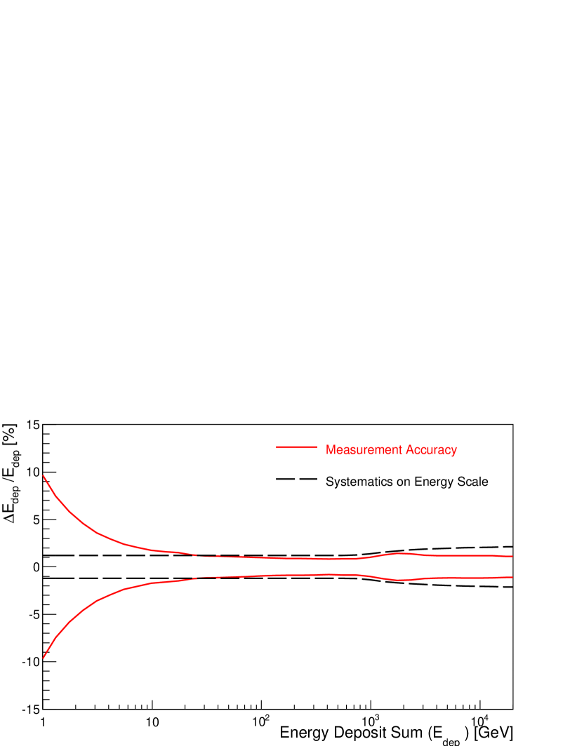
Figure 11: (Top) Energy dependence of the relative error in the energy deposit sum measurements for electrons, considering all the energy calibration errors and detector responses (solid red lines). The systematic uncertainty on an absolute scale is also shown by black dashed lines. (Bottom) Estimated energy resolution for electrons as a function of energy. Open red squares denote intrinsic resolution and closed red squares denote actual resolution including all the detector responses and calibration errors in the case of energy determination using the TASC$+$IMC. Circular symbols indicate energy determination using the TASC only.

To conclude, the estimated energy resolution for electrons as a function of energy is plotted in the bottom panel of Fig. 11. Thanks to the detailed calibration process described in this paper, a very high energy resolution has been achieved over the entire dynamic range.

6 Conclusion

Energy calibration of the CALET, launched to the ISS in August 2015 and accumulating scientific data since October 2015, was performed using both flight data and calibration data acquired on the ground before launch. By taking advantage of the fully-active total absorption calorimeter, absolute calibration between ADC units and energy was possible with an accuracy of a few percent, using penetrating particles. Successful calibration was achieved over the complete dynamic range of six orders of magnitude for each TASC channel with sufficient accuracy to maintain a fine resolution of 2% above 100 GeV by combining two calibration processes: linearity measurements over each gain range and determination of the correlation between adjacent gain ranges. The systematic error in the energy scale was also estimated based on the calibration results and was found to be $\leq$ 2%. Based on long duration observations of high energy cosmic rays onboard the ISS, the measurement of the inclusive ($e^{+}+e^{-}$) electron spectrum well into the TeV region with unprecedented accuracy is expected, as well as measurements of gamma-rays, protons and nuclei.

References

- [1] S. Torii et al., “The CALorimetric Electron Telescope (CALET): High Energy Astroparticle Physics Observatory on the International Space Station”, Proceedings of Science, Proc. of the 34th ICRC (The Hague, Netherlands), 1.
- [2] Y. Asaoka et al., “Development of the Waseda CALET Operations Center (WCOC) for Scientific Operations of CALET”, Proceedings of Science, Proc. of the 34th ICRC (The Hague, Netherlands), 603.
- [3] T. Kobayashi et al., “The most likely sources of high-energy cosmicray electrons in supernova remnants”, Astrophys. J. 601 (2004) 340.
- [4] N. Kawanaka et al., “TeV electron spectrum for probing cosmic-ray escape from a supernova remnant”, Astrophys. J. 729 (2011) 93.
- [5] H. Motz, Y. Asaoka, S. Torii and S. Bhattacharyya, “CALET’s sensitivity to Dark Matter annihilation in the galactic halo”, JCAP 2015 (2015) 12, 047.
- [6] O. Adriani et al., “Cosmic-ray electron flux measured by the PAMELA experiment between 1 and 625 GeV”, Phys. Rev. Lett. 106 (2011) 201101.
- [7] M. Aguilar et al., “Precision Measurement of the Flux in Primary Cosmic Rays from 0.5 GeV to 1 TeV with the Alpha Magnetic Spectrometer on the International Space Station”, Phys. Rev. Lett. 113 (2014) 221102.
- [8] J. Chang et al., “An excess of cosmic ray electrons at energies of 300–800 GeV”, Nature 456 (2008) 362.
- [9] A.A. Abdo et al., “Measurement of the Cosmic Ray Spectrum from 20 GeV to 1 TeV with the Fermi Large Area Telescope”, Phys. Rev. Lett. 102 (2009) 181101; M. Ackermann et al., “Fermi LAT observations of cosmic-ray electrons from 7 GeV to 1 TeV”, Phys. Rev. D 82 (2010) 092004.
- [10] P.S. Marrocchesi, et al., “CALET measurements with cosmic nuclei and performance of the charge detectors”, Proc. of 33nd International Cosmic Ray Conference (Rio de Janeiro). ID#0362.
- [11] T. Niita et al., “Energy calibration of Calorimetric Electron Telescope (CALET) in space”, Adv. Space Res. 55 (2015) 2500.
- [12] Y. Akaike et al., “Expected CALET Telescope Performance from Monte Carlo Simulations”, Proc. of the 32nd ICRC (Beijing, China), Vol.6, (2011) 371.
- [13] M. Honda et al., “New calculation of the atmospheric neutrino flux in a tree-dimensional scheme”, PRD 70 (2004) 043008.
- [14] M. Aguilar et al., “The Alpha Magnetic Spectrometer (AMS) on the International Space Station: Part I – results from the test flight on the space shuttle”, Phys. Rep. 366 (2002) 331.
- [15] T. Sanuki et al., “PRECISE MEASUREMENT OF COSMIC-RAY PROTON AND HELIUM SPECTRA WITH THE BESS SPECTROMETER”, Astrophys. J. 545 (2000) 1135.
- [16] K. Kasahara, “Introduction to cosmos and some relevance to ultra high energy cosmic ray air showers”, Proc. of 24th International Cosmic Ray Conference (Rome, Italy), Vol. 1 (1995) 399; “EPICS Home Page” http://cosmos.n.kanagawa-u.ac.jp/EPICSHome/.
- [17] M. Karube et al., “Performance of the CALET Prototype: CERN Beam Test” Proc. of the 32nd ICRC (Beijing, China), Vol.6, (2011) 383.