OLÉ: Orthogonal Low-rank Embedding,
A Plug and Play Geometric Loss for Deep Learning

Abstract

Deep neural networks trained using a softmax layer at the top and the cross-entropy loss are ubiquitous tools for image classification. Yet, this does not naturally enforce intra-class similarity nor inter-class margin of the learned deep representations. To simultaneously achieve these two goals, different solutions have been proposed in the literature, such as the pairwise or triplet losses. However, such solutions carry the extra task of selecting pairs or triplets, and the extra computational burden of computing and learning for many combinations of them. In this paper, we propose a plug-and-play loss term for deep networks that explicitly reduces intra-class variance and enforces inter-class margin simultaneously, in a simple and elegant geometric manner. For each class, the deep features are collapsed into a learned linear subspace, or union of them, and inter-class subspaces are pushed to be as orthogonal as possible. Our proposed Orthogonal Low-rank Embedding (OLÉ) does not require carefully crafting pairs or triplets of samples for training, and works standalone as a classification loss, being the first reported deep metric learning framework of its kind. Because of the improved margin between features of different classes, the resulting deep networks generalize better, are more discriminative, and more robust. We demonstrate improved classification performance in general object recognition, plugging the proposed loss term into existing off-the-shelf architectures. In particular, we show the advantage of the proposed loss in the small data/model scenario, and we significantly advance the state-of-the-art on the Stanford STL-10 benchmark.

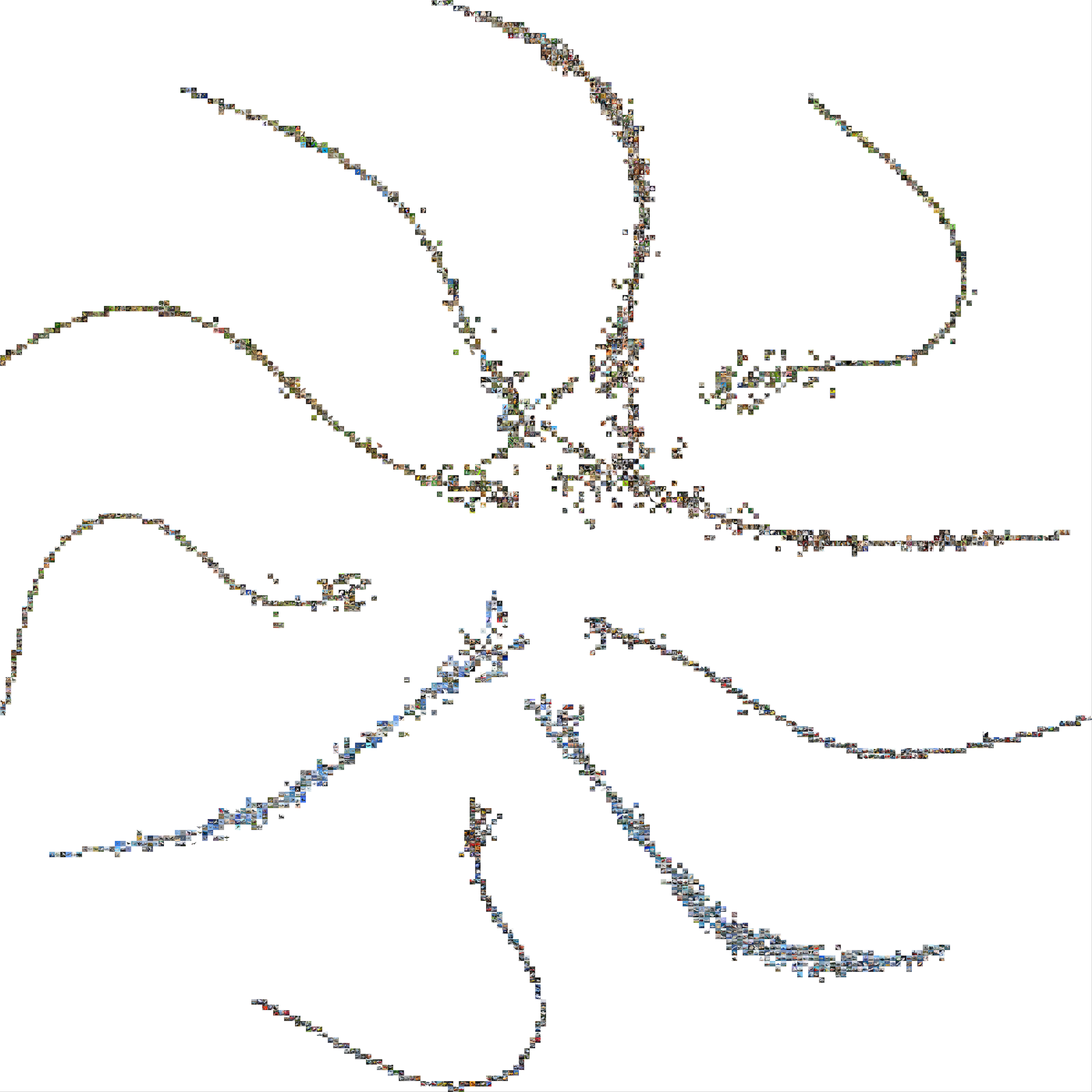
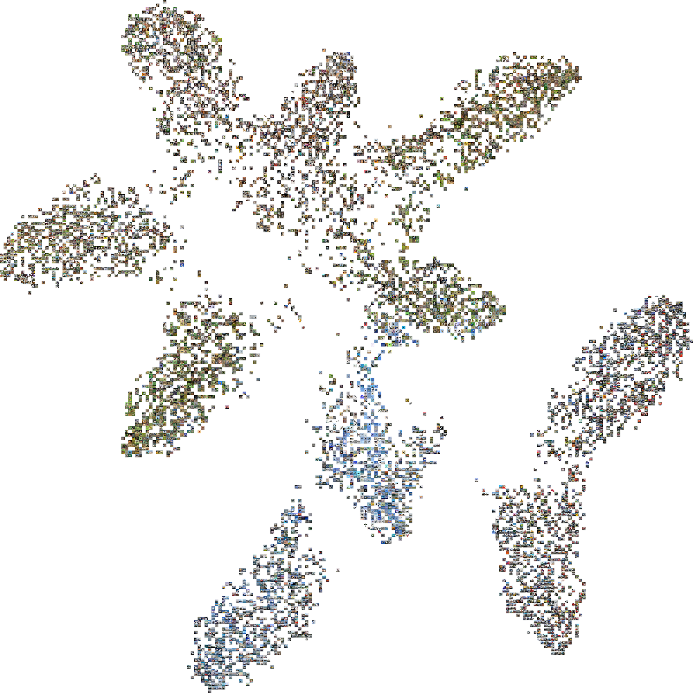
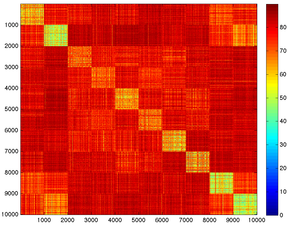
(a)	(b)	(c)	(d)

Figure 1: Barnes-Hut-SNE [32] visualization of the deep feature embedding learned for the validation set of CIFAR10, using VGG-16. (a) With softmax loss and OLÉ . (b) With softmax loss only. The separation between classes is increased, and a low-rank structure is recovered for each class. (c) Angle between the features of the 10,000 validation samples, ordered by class, with OLÉ. (d) Without OLÉ. With OLÉ the angle between features is collapsed inside each class and inter-class features are orthogonal. Best viewed in electronic format.

(a) OLÉ: 78.38% accuracy	(b) Softmax: 76.69% accuracy	(c) OLÉ: 100.0% accuracy	(d) Softmax: 96.47% accuracy
CIFAR 3 classes		Facescrub 3 classes

Figure 2: Illustrative comparison between OLÉ loss (standalone) and softmax loss. We show the actual 3D deep feature vectors for the validation images in two 3-class classification problems with scarce training data. OLÉ produces intra-class compactness and inter-class orthogonality, and is able to achieve better classification performance than the softmax loss. (a) & (b) 3 classes of CIFAR10, trained with 1,000 images per class. A 4 layer, 100 hidden units MLP was used. (c) & (d) 3 subjects of Facescrub dataset, trained with 110 images per class on average. A 3 layer, 10 hidden units MLP was used. See text for more details. Best viewed in electronic format.

1 Introduction

In the last few years the representational power of Deep Neural Networks (DNNs) has been thoroughly demonstrated, with impressive results in learning useful representations for difficult tasks such as object classification and detection [6, 8, 11, 15, 29] and face identification and verification [22, 28, 35], to name just a few examples. DNNs typically consist of a sequence of convolutional and/or fully-connected layers with non-linear activation functions, which produce a “deep” feature vector, which is then classified in the last layer with a linear classifier [8, 11, 15, 29]. This linear classifier typically uses the softmax function with the cross-entropy loss. The combination of these two will be referred to as softmax loss in the rest of this article. The layer previous to the last linear classifier will be referred to as the deep feature layer.

Training a DNN with the standard softmax loss does not explicitly enforce an embedding of the learned deep features where samples of the same class are closer together and further away from other classes. To improve the discrimination power of deep neural networks, previous approaches have tried to enforce such an embedding via auxiliary supervisory loss functions [16] acting on the Euclidean distances between the deep features [1, 5, 10, 28, 30, 35]. Such metric learning techniques are particularly popular in the face identification domain, with its two most representative examples being the pairwise loss [5] and the triplet loss [28]. The drawback with these approaches is that they require the careful selection of pairs or triplets of samples, as well as extra data processing. More recently, methods have been proposed to overcome this limitation by enforcing intra-class compactness of the representations inside each random training minibatch, [17, 18, 35].

In this work we propose to improve the discriminability of a neural network by a simple and elegant plug-and-play loss term that, acting on the deep feature layer, encourages the learned deep features of the same class to lie in a linear subspace (or union of them), and at the same time that inter-class subspaces are orthogonal, see Figs. 1, 2. To the best of our knowledge, this is the first time a deep learning framework is proposed that simultaneously reduces intra-class variance and increases inter-class margin, without requiring pair or triplet selection.

Our intuition is based on the following observations. First, that the decision boundary for the softmax loss is determined by the angle between the feature vector and the vectors corresponding to each class in the last linear classifier [18]. Since the weights are initialized randomly, the class vectors are, with high probability, orthogonal at initialization, and typically remain so after training. Moreover, if a rectified linear unit (ReLU) is the last activation function, the deep features will live in the positive orthant. Therefore, one way to improve the margin between deep features is to embed them into orthogonal, low-dimensional linear subspaces, aligned with the classifier vector of each class.

To this end, we adapt a shallow feature orthogonalization technique [25] to deep networks. Through novel theoretical insight, we improve the objective formulation in [25] and its optimization. The outcome is a new loss function that can be plugged into any existing deep architecture at the deep feature layer. We demonstrate via thorough experimentation that this approach produces orthogonal deep representations that lead to better generalization, not only in face identification but also in general object recognition. We illustrate this on different datasets and using four of the most popular CNN architectures: VGG [29], ResNets [8], PreResNets [9] and DenseNets [11].

We demonstrate that our proposed technique is particularly successful in the small data scenario. We significantly advance the state-of-the-art in the STL-10 standard benchmark [3] when training with only 500 images per class, and show that the advantage of OLÉ over the standard softmax loss increases as fewer training samples are used. We also show through a face recognition application that because of the improved discriminability, the network is better at detecting novel classes (outside the training set).

The source code for OLÉ is publicly available.

This paper is organized as follows. In Section 2 we discuss related work on similarity preserving and large margin deep networks. In Section 3 we motivate and describe the orthogonalization loss and its optimization, as well as a warming-up example. Experimental results are presented in Section 4. We conclude the paper in Section 5

2 Related Work

The first attempts to reduce the intra-class similarity of deep features and increase their inter-class separation are metric learning based approaches [1, 5, 10, 28, 30, 35]. Their goal is to minimize the Euclidean distance between the deep features of the same class, while keeping the other classes apart. The pioneering contrastive loss [5] imposes such constraint using a siamese network architecture [2]. This pairwise strategy was particularly popular in the face identification community [5, 30, 10], and was later extended to a triplet loss [28, 1]. With the triplet loss, an image representation is simultaneously enforced to be close to a positive example of the same class and far away from a negative example of a different class. The main drawback of these approaches is that they require carefully mining for pairs or triplets that effectively enforce the constraints.

A different strategy to encourage intra-class compactness was proposed in [35], where a centroid for the deep representation of each class is updated in each training iteration, and Euclidean distances to the centroids are penalized. This simple strategy produces compact clusters for each class, although a large margin between clusters is not explicitly enforced. Contrary to our method, the center loss cannot be used standalone as a classification loss, since all the centroids tend to collapse to zero [35]. A related approach in [27] estimates a distribution for the representation of each class and penalizes class distribution overlap.

Based on the observation that the softmax loss is a function of the angles between deep features and classifier vectors, a novel family of methods have been proposed in [17, 18], that operate on such angles and not on Euclidean distances. These works propose custom versions of the softmax loss that encourage the features of one class to have a smaller angle with their corresponding classification vector than in the standard softmax loss. The improved margin produces notorious performance boosting with respect to a standard network [17, 18].

In the unsupervised learning domain, a very recent family of methods proposes to enforce a locally linear structure in the deep representations, such that Subspace Clustering [33] can be later applied to the deep representations [13, 23]. These properties will arise naturally in the deep representations learned with OLÉ, although imposed in a supervised manner.

Our work is related to [17, 18, 35], in that we enforce intra-class compactness inside each minibatch. However, for the first time, our objective function also simultaneously encourages inter-class orthogonality, without the need to carefully craft pairs or triplets.

This work stems from an orthogonalization technique used for shallow learning proposed in [25]. The orthogonalization is achieved via a linear transformation enforcing a low-rank constraint on the features of the same class, and a high-rank constraint on the matrix of features of all classes. More precisely, consider a matrix $\mathbf{Y}=\left[\mathbf{y}_{1}~{}|~{}\mathbf{y}_{2}~{}|~{}\ldots~{}|~{}\mathbf{y}_{N}\right]$, where each column $\mathbf{y}_{i}\in\mathbb{R}^{d},i=1,\ldots,N$ is a data point from one of the $C$ classes, and $|$ denotes horizontal concatenation. Let $\mathbf{Y}_{c}$ denote the submatrix formed by the columns of $\mathbf{Y}$ that lie in the $c$-th class. In [25], a linear transform $\mathbf{T}:\mathds{R}^{d}\rightarrow\mathds{R}^{d}$ is learned to minimize

$${\sum_{c=1}^{C}||\mathbf{TY}_{c}||_{*}-||\mathbf{TY}||_{*},~{}~{}\mathrm{s.t.}||\mathbf{T}||_{2}=1,}$$ (1)

where $||\mathbf{\cdot}||_{*}$ denotes the matrix nuclear norm, i.e., the sum of the singular values of a matrix. The nuclear norm is the convex envelope of the rank function over the unit ball of matrices [26]. An additional condition $||\mathbf{T}||_{2}=1$ is originally adopted to prevent the trivial solution $\mathbf{T}=0$.

Here we adapt the loss in (1) to the deep learning framework and reformulate the loss and its optimization in a manner that is suitable for training by backpropagation.

3 Orthogonalization Loss

3.1 Motivation

Consider a neural network whose last fully connected layer is $\mathbf{W}\in\mathds{R}^{C\times D}$, where $D$ is the dimension of the deep features and $C$ the number of classes. Each row $\mathbf{w}_{c}\in\mathds{R}^{D}$ of $\mathbf{W}$ represents a linear classifier for class $c$. If $\mathbf{W}$ is initialized randomly, then such rows are (with high probability) orthogonal. Now consider $\mathbf{x}$ as the deep representation of an image (or any other data being classified). If the activation function in the deep feature layer is the element-wise maximum between $\mathbf{x}$ and $0$ (ReLU), then $\mathbf{x}$ always lives in the positive orthant. From these two observations it can be deduced that at the end of a successful training of the network the classifier vectors $\mathbf{x}_{c}$ should remain orthogonal to have the most separation between classes. Therefore, one strategy to learn large-margin deep features is to make the intra-class features fall in a linear subspace aligned with the corresponding classification vector, while features of different classes should be orthogonal to each other. This natural geometry of learned features is not imposed by standard last-layer classifiers in today’s leading architectures.

3.2 Definition

We propose to enforce the aforementioned orthogonalization by adapting (1) to the deep learning setting. Namely, suppose for a given training minibatch $\mathbf{Y}$ of $N$ samples, $\mathbf{X}=\Phi(\mathbf{Y};\mathbf{\theta})$ is the $N\times D$ deep embedding $\Phi$ of the data, parameterized by $\mathbf{\theta}$.

Let $\mathbf{Y}_{c}$, $\mathbf{X}_{c}$ be the data and the sub-matrix of deep features belonging to class $c$, respectively, and $\mathbf{X}$ the matrix of deep features for the entire minibatch $\mathbf{Y}$. We propose the following OLÉ loss:

$$\mathbf{L}_{o}(\mathbf{X}) :={{\sum_{c=1}^{C}\max(\Delta,||\mathbf{X}_{c}||_{*})-||\mathbf{X}||_{*}}}$$ (2)

$$={{\sum_{c=1}^{C}\max(\Delta,||\Phi(\mathbf{Y}_{c};\theta)||_{*})-||\Phi(\mathbf{Y};\theta)||_{*}}}$$ (3)

With respect to (1), we drop the linear transformation $T$ (the network is already transforming the data) and its normalization restriction, and we add a bound $\Delta\in\mathds{R}$ on the intra-class nuclear loss, so that after a certain point the intra-class norm reduction is no longer enforced, thus avoiding the collapse of the features to zero (and therefore no needing the normalization). We will always use $\Delta=1$ for the experiments in this paper.

The global minimum of (2) is reached when each of the $\mathbf{X}_{c}$ matrices are orthogonal to each other [25]. We next describe a simple descent direction for optimizing $\mathbf{\theta}$ (2) via backpropagation, and show that this direction vanishes only when the orthogonalization is achieved.

3.3 Optimization

In order to optimize (2) via backpropagation, we need to compute a subgradient of the nuclear norm of a matrix. Let $\mathbf{A}=\mathbf{U}\mathbf{\Sigma}\mathbf{V}^{T}$ be the SVD decomposition of the $m\times n$ matrix $\mathbf{A}$. Let $\delta$ be a small threshold value, and $s$ the number of singular values of $\mathbf{A}$ larger than $\delta$. Let $\mathbf{U}_{1}$ be the first $s$ columns of $\mathbf{U}$ and $\mathbf{V}_{1}$ be the first $s$ columns of $\mathbf{V}$ (corresponding to those larger than $\delta$ eigenvalues). Correspondingly, let $\mathbf{U}_{2}$ be the remaining columns of $\mathbf{U}$ and $\mathbf{V}_{2}$ the remaining columns of $\mathbf{V}$. Then, a subdifferential of the nuclear norm is ([26, 34])

$$\partial{||\mathbf{A}||_{*}}=\mathbf{U}_{1}\mathbf{V}_{1}^{T}+\mathbf{U}_{2}\mathbf{W}\mathbf{V}_{2}^{T},$$ (4)

with $||\mathbf{W}||\leq 1$.

Here we propose to use $\mathbf{W}=0$, obtaining the following projected subgradient for the nuclear norm minimization problem:

$$g_{||A||_{*}}(A)=\mathbf{U}_{1}\mathbf{V}_{1}^{T}.$$ (5)

Intuitively, to avoid numerical issues, we are dropping the directions of the subgradient onto which the data matrix has no or very low energy already (i.e., their corresponding singular values are already close to 0). This improves upon the formulation in [25], where all the directions were used.

Suppose $\mathbf{X}=\left[\mathbf{X}_{1}~{}|~{}\mathbf{X}_{2}~{}|~{}\ldots~{}|~{}\mathbf{X}_{C}\right]$ is the deep feature matrix of one minibatch. For $\mathbf{X}_{c}$, the feature submatrix of each class $c\in\{1,\ldots,C\}$, let $\mathbf{U}_{1c}$ and $\mathbf{V}_{1c}$ be its principal left and right singular vectors. Let $\mathbf{U}_{1}$ and $\mathbf{V}_{1}$ be the principal left and right singular vectors of $\mathbf{X}$, the deep feature matrix of all the classes combined. (By principal we mean those whose corresponding singular value is greater than the threshold $\delta$.) Then, we propose the following descent direction for (2):

$$g_{L_{o}}(\mathbf{X}):=\sum_{c=1}^{C}\left[\mathbf{Z}_{c}^{(l)}~{}|~{}\mathbf{U}_{c1}\mathbf{V}_{c1}^{T}~{}|~{}\mathbf{Z}_{c}^{(r)}\right]-\mathbf{U}_{1}\mathbf{V}_{1}^{T}.$$ (6)

Here, $\mathbf{Z}^{(l)}_{c}$ and $\mathbf{Z}^{(r)}_{c}$ are fill matrices of zeros to complete the dimensions of $\mathbf{X}$. The first term in (6) reduces the variance of the principal components of the per-class features. The second term increases the variance of all the features together, projecting the feature matrix onto its closest orthogonal form.

Next we prove that this direction vanishes only when the objective reaches the global minimum of zero.

Proposition 1.

If $g_{L_{o}}(\mathbf{X})=0$ and $||X_{c}||_{*}>\Delta$, then $L_{o}(\mathbf{X})=0$.

Proof.

We give the proof for two classes, its extension to multiple classes is straightforward. Let $\mathbf{X}=\left[\mathbf{A}~{}|~{}\mathbf{B}\right]$ with $\mathbf{A}$ and $\mathbf{B}$ corresponding to the feature matrices of two classes. Let $\mathbf{A}=\mathbf{U}_{A1}\mathbf{\Sigma}_{A1}\mathbf{V}_{A1}+\mathbf{U}_{A2}\mathbf{\Sigma}_{A2}\mathbf{V}_{A2}$ and $\mathbf{B}=\mathbf{U}_{B1}\mathbf{\Sigma}_{B1}\mathbf{V}_{B1}+\mathbf{U}_{B2}\mathbf{\Sigma}_{B2}\mathbf{V}_{B2}$ be their SVD decomposition, where the subscript $1$ corresponds to the singular values larger than the threshold $\delta$ and the subscript $2$ to the remaining singular values. Let $\mathbf{0}$ be a generic matrix of zeroes, whose size is determined by context, for simplicity. Then,

$$L_{o}(\mathbf{X})=||A||_{*}+||B||_{*}-||[A~{}|~{}B]||_{*},$$ (7)

$$g_{L_{o}}(\mathbf{X})=\left[\begin{array}[]{c|c}\mathbf{U}_{A1}\mathbf{V}_{A1}^{T}&\mathbf{0}\end{array}\right]+\left[\begin{array}[]{c|c}\mathbf{0}&\mathbf{U}_{B1}\mathbf{V}_{B1}^{T}\end{array}\right]-\mathbf{U}_{1}\mathbf{V}_{1}^{T}.$$ (10)

Then, $g_{L_{o}}(\mathbf{X})=0$ implies

$$\mathbf{U}_{1}\mathbf{V}_{1}^{T} =\left[\begin{array}[]{c|c}\mathbf{U}_{A1}\mathbf{V}_{A1}^{T}&\mathbf{0}\end{array}\right]+\left[\begin{array}[]{c|c}\mathbf{0}&\mathbf{U}_{B1}\mathbf{V}_{B1}^{T}\end{array}\right]$$ (13)

$$=\left[\begin{array}[]{c|c}\mathbf{U}_{A1}&\mathbf{U}_{B1}\end{array}\right]\left[\begin{array}[]{c|c}\mathbf{V}_{A1}^{T}&\mathbf{0}\\ \mathbf{0}&\mathbf{V}_{B1}^{T}\end{array}\right].$$ (17)

Since $\mathbf{U}_{1}$ and $\mathbf{V_{1}}$ are orthogonal matrices, and the rightmost matrix in (17) is also orthogonal, then $\left[\mathbf{U}_{A1}~{}|~{}\mathbf{U}_{B1}\right]$ must be orthogonal. Since $\mathbf{U}_{A1}$ and $\mathbf{U}_{B1}$ are orthogonal submatrices, this implies that their columns must be orthogonal to each other. Then, $\mathbf{A}$ and $\mathbf{B}$ are orthogonal to each other and thus $L_{o}(\mathbf{X})=0$ [25] (Theorem 2).

∎

In practice, we observe empirical convergence in all our experiments. Fig. 3 shows typical convergence curves for the OLÉ loss when used standalone or in combination with the softmax loss.

3.4 Illustrative Example

In Fig. 2 we show via two simple illustrative examples the result of applying the OLÉ loss of (2) as the objective function of a neural network. We compare with the result of applying the traditional softmax loss.

For the first experiment, we used 3 classes from CIFAR10 (0: plane, 1: car, 2: bird) and trained a Multi-Layer Perceptron (MLP), with 4 hidden layers of 100 neurons each, and a final layer of dimension 3. The network was trained for 300 epochs on 1,000 images per class and evaluated in 100 images per class.

For the second experiment, we used 3 randomly chosen subject identities from the Facescrub dataset [21]: Al Pacino, Helen Hunt, and Sean Bean. Each identity contains, on average, 110 images for training and 30 for validation. We used a 3 layer MLP with 10 neurons in each hidden layer, and trained for 150 epochs. All the MLPs use ReLU activation functions, batch normalization and weight decay and were trained with Adam with learning rate $10^{-4}$.

For the comparison, the architecture and hyperparameters are shared and only the objective function is changed. For evaluation, we use 1-Nearest-Neighbor with cosine distance, (this yielded equivalent or better performance than using the softmax score). We ran the training 50 times for each architecture and dataset and kept the model giving the best classification result in the validation set.

In Fig. 2 we plot the actual 3D deep feature vectors obtained by the networks for the validation set. We observe a successful orthogonalization of the learned features when using OLÉ and a better classification performance, in particular for the Facescrub experiments, where the number of samples per class is very limited.

In the following section, we will combine the power of the OLÉ and the softmax loss to achieve significant performance gains, in particular in the small data scenario.

3.5 Discussion

The proposed embedding has several advantages with respect to similar embeddings in the literature:

• It does not require carefully crafting pairs or triplets of samples, and works simply as a plug-and-play loss that can be appended to any existing network architecture.

• Compared to the Large-Margin Softmax Loss in [18] or the A-softmax loss in [17], the OLÉ loss is not restricted to be used with a softmax classifier and can be used standalone or as a complement of any other loss, or to impose orthogonality at any layer of the network.

• Compared to the Center Loss of [35], our deep objective function encourages intra-class compactness and inter-class separation simultaneously, whereas [35] does only the former. Also, the Center Loss cannot be used standalone.

• OLÉ collapses the deep features into linear subspaces. When used in conjunction with the softmax loss, the linear classifiers of the last layer find a natural form which is a vector aligned with the linear subspace.

4 Experimental Evaluation

In this section, we demonstrate the improved generalization performance obtained when using the OLÉ loss in combination with the standard softmax loss for several popular deep network architectures and different standard visual classification datasets. We will also further analyze the effect of the proposed embedding.

In all experiments, we seek to minimize the combination of the softmax classification loss and the OLÉ loss:

$$\underset{\mathbf{\theta}}{\min}~{}{L_{s}}(\mathbf{X},\mathbf{y},\mathbf{\theta})+\lambda\cdot{L_{o}}(\mathbf{X},\mathbf{y},\mathbf{\theta}^{*})+\mu\cdot||\mathbf{\theta}||^{2},$$ (18)

where $L_{S}$ is the standard softmax loss (softmax layer plus cross-entropy loss). The second term $L_{o}$ is the proposed OLÉ loss (2). The parameter $\lambda$ controls the weight of the OLÉ loss; $\lambda=0$ corresponds to standard network training.

Here $\mathbf{\theta}^{*}$ means every weight in the network except the weights of the last fully-connected layer, which is the linear classifier. This is because the OLÉ loss is applied to the deep features at the penultimate layer. The third term represents the standard weight decay. The values used for these parameters are detailed below.

4.1 Datasets

SVHN. The Street View House Numbers (SVHN) dataset [20] contains $32\times 32$ colored images of digits 0 to 9, with $73,257$ images for training and 26,032 for testing. We did not use the additional unlabeled training images nor performed any data augmentation.

MNIST. The MNIST database contains $28\times 28$ grayscale images of digits from 0 to 9. The training and testing set contain 60,000 and 10,000 examples respectively. No data augmentation was used.

CIFAR10 and CIFAR100. The two CIFAR datasets [15] contain $32\times 32$ colored images from 10 and 100 object classes respectively. Both datasets contain 50,000 images for training and 10,000 for testing. When using data augmentation, we append the suffix ’+’ to the dataset name. We used the standard data augmentation for CIFAR: 4 pixel padding, $32\times 32$ random cropping and horizontal flipping.

STL-10. The Self-Taught Learning 10 (STL-10) dataset [3] contains $96\times 96$ colored images from 10 object categories. Designed for semi-supervised and unsupervised learning, there are only $500$ training images and $800$ test images with labels per class. Data augmentation consisted of 12 pixel padding, and random $96\times 96$ cropping and horizontal flipping. We add the ’+’ suffix when reporting results using data augmentation.

VGG-11	C64-MP-C128-MP-C256(x2)-MP-C512(x2)-MP-C512(x2)-MP-FC512
VGG-16	C64(x5)-MP-C128(x4)-MP-C256(x4)-MP-FC256
VGG-19	C64(x2)-MP-C128(x2)-MP-C256(x4)-MP-C512(x4)-MP-C512(x4)-MP-FC512
VGG-FACE	C64(x2)-MP-C128(x2)-MP-C256(x3)-MP-C512(x3)-MP-C512(x3)-FCD4096(x2)-FC1024
ResNet-110	C16-R64/16(x18)-R128/32(x18)-R256/64(x18)-AP
Pre-ResNet-110	C16-PR64/16(x18)-PR128/32(x18)-PR256/64(x18)-BN-ReLU-AP
DenseNet-40-12	CO24-D168/12-CR168-D312/12-CR312-D456/12-BN456-ReLU
CNN-5	C32-MP-C64-MP-C128-MP-C256-C256-MP

Table 1: Summary of the deep network architectures used in our experiments. The last Fully-Connected layer, whose size depends on the number of classes used, is not shown. CX: Convolutional block. Kernel size is always is 3x3. MP: Max pooling with kernel size 2x2 and stride 2. FCX: Fully-Connected layer. RX/Y and PRX/Y: ResNet and PreResNet Blocks Respectively. AP: Global Average Pooling layer. COX: Plain convolutional layer. DX/G: DenseNet Block. PCX: Pre-BN convolutional block: (BN-conv.-ReLU). Kernel size is 1x1. For all the modules, X is the number of output channels. Y is the number of inner channels for R and PR blocks and G is the growth rate for D blocks. See text for detailed block definitions. The OLÉ loss is always applied at the output of the last layer shown in this table.

Facescrub-500. The Facescrub-500 dataset is obtained by selecting 500 of the 530 identities of the Facescrub dataset [21]. The remaining 30 classes were used for evaluating out of sample performance. We split the images of the first 500 subjects into a training and a testing datasets with on average $91$ images for training and $23$ images for testing per class (80%/20% split). We preprocess the images by aligning facial landmarks using [14] and crop the resulting aligned face images to $224\times 224$, with color.

4.2 Network Architectures

Evaluated architectures are summarized in Table 1.

VGG. The VGG architecture [29] consists of blocks of convolutional layers with ReLU activation functions and Batch Normalization (BN), linked by Max-Pooling layers and with one or more fully-connected (FC) layers at the end. For VGG-11 and VGG-19 we use a publicly available implementation. For VGG-16, we used the implementation from [18] to allow for a more direct comparison.

VGG-FACE. VGG-FACE is a variant of VGG optimized for face identification [22]. In VGG-FACE, the convolutional blocks do not have BN and the first two FC layers use Dropout with rate 0.5. We added an FC layer of size 1024, that was not present in [22]. This layer improves performance for all tested models on Facescrub-500. We used the Caffe implementation of the authors and fine-tune the weights provided by them. The novel 1024 FC layer was initialized using “Xavier” initialization [4].

ResNet and PreResNet. ResNets [8] are composed of residual blocks. The concatenation of layers inside a ResNet block is conv.-BN-conv.-BN-conv.-BN-ReLU. The intermediate convolution layers typically have one fourth the number of channels than the input and output convolution layers of a block, see Table 1. The output of each block is added to its input. The PreResNet architecture [9] is similar to ResNet except that inside the residual blocks the order of the layers is inverted: BN-conv.-BN-conv.-BN-conv.-ReLU. No Dropout is used. For both variants we used a publicly available implementation.

DenseNet. DenseNets [11] are composed of three DenseNet blocks. Each of these blocks is itself composed of multiple pre-BN convolutional blocks (BN-conv.-ReLU) with a small number of output channels. Inside a DenseNet block, the input to each pre-BN convolutional block is the concatenation of the output of all previous pre-BN convolutional blocks. A transition pre-BN convolutional block is used between DenseNet blocks. In our experiments, no bottleneck layers were used. We used Dropout of 0.2 for MNIST and SVHN, and no Dropout for CIFAR. We used a publicly available implementation.

4.3 Training Details

Except for the Facescrub experiments, we always train the network from scratch. VGG-16 uses “MSRA” initialization [7]. For the rest of the architectures, “Xavier” initialization was used [4].

In all the experiments except STL-10 and Facescrub we used SGD with Nesterov momentum 0.9 for the optimization and batch size 64. We started with a learning rate of 0.1 and decreased it ten-fold at 50% and 75% of the total training epochs. For STL-10/Facescrub experiments, we used Adam with starting learning rate $10^{-3}$/$10^{-5}$ and batch size 32/26. We used 164 epochs for all architectures except for DenseNets, for which we used 300 epochs and Facescrub where the finetuning is done for 12 epochs. The weight decay parameter was always set to $\mu=10^{-4}$, except for STL-10+ and Facescrub, where $\mu=10^{-3}$. Fig. 3 shows typical convergence curves.

We implemented the OLÉ loss as a custom layer for Caffe and PyTorch. The additional computation time is between 10% and 33% during training, depending on the implementation and hardware, because the SVD runs on the CPU in the current implementation.

We adjusted the parameter $\lambda$ in (18) with a held-out validation set of 10% of the training set. Note that the magnitude of the OLÉ loss depends on the size and norm of the features matrices. We selected the value of $\lambda$ that produced the best result in the validation set, averaging over 5 runs, see Fig 4 for an example. We then retrained the network with the entire training set and we computed the accuracy on the test set at the end of the training. To account for the randomness of the training process, we repeated the training with the full training set 5 times.

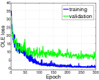
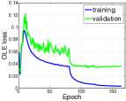
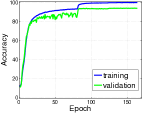
(a)	(b)	(c)

Figure 3: Learning curves. (a) OLÉ loss when used standalone. Data and model from Fig 2c. (b) & (c) OLÉ loss and accuracy when used in combination with softmax loss for a ResNet-110 on CIFAR10+. Learning rate drops by 0.1 at 81 and 122 epochs.

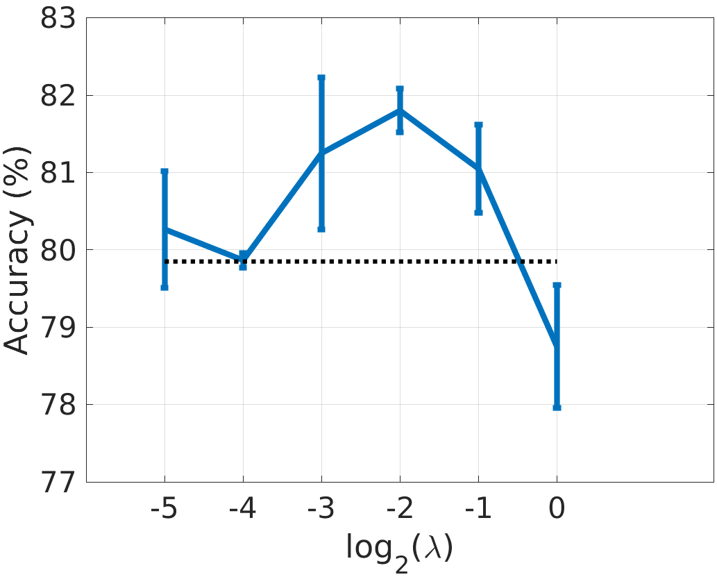
Figure 4: Validation of $\lambda$ (18) for the STL-10+ experiment. Based on this graph, we chose $\lambda=0.25$ for the final training. The dotted line is the average score obtained with the standard softmax loss.

4.4 Visual Classification Results

Dataset	Architecture	$\lambda$	% Error ($L_{o}+\lambda\cdot L_{s})$	% Error ($L_{s}$ only)	Ref. Error (%)
SVHN	DenseNet-40-12 [11]	$1/2$	$\mathbf{3.62}\pm 0.04$	$3.93\pm 0.08$	$1.79$ [11]
MNIST	DenseNet-40-12	$1/2$	$\mathbf{0.78}\pm 0.04$	$0.88\pm 0.03$	-
CIFAR10+	DenseNet-40-12	$1/8$	$\mathbf{5.30}\pm 0.26$	$5.54\pm 0.13$	$5.24$ [11]
CIFAR10+	ResNet-110 [8]	$1/4$	$\mathbf{5.39}\pm 0.25$	$6.05\pm 0.8$	$6.43$ [8]
CIFAR10+	VGG-19 [29]	$1/4$	$\mathbf{7.13}\pm 0.2$	$7.37\pm 0.11$	-
CIFAR10+	VGG-11	$1/2$	$\mathbf{7.73}\pm 0.14$	$8.06\pm 0.22$	-
CIFAR10	VGG-16 [18]	$1/2$	$\mathbf{7.22}\pm 0.14$	$8.23\pm 0.13$	$7.58$ [18]
CIFAR100+	PreResNet-110 [9]	$1/20$	$\mathbf{22.8}\pm 0.34$	$23.01\pm 0.19$	$22.68\pm 0.22$ [9]
CIFAR100+	VGG-19	$1/10$	$\mathbf{27.54}\pm 0.11$	$28.04\pm 0.42$	-
CIFAR100	VGG-19	$1/10$	$\mathbf{37.25}\pm 0.33$	$38.15\pm 0.28$	-
FaceScrub-500	VGG-FACE [22]	$250$	$\mathbf{1.55}\pm 0.02$	$2.49\pm 0.01$	-
STL-10	CNN-5	$1/16$	$\mathbf{25.42}\pm 0.20$	$28.68\pm 0.67$	-
STL-10+	CNN-5	$1/4$	${\color[rgb]{0,0,1}\mathbf{16.68}}\pm 0.24$	$18.22\pm 0.27$	$21.34$ [31]

Table 2: Visual classification results. $L_{o}$ is the proposed OLÉ loss, $L_{s}$ is the standard softmax loss.

Table 2 shows the resulting classification performance, with and without OLÉ. In all the experiments, we found a value of $\lambda$ through validation such that the generalization of the network is improved. For reference, we include in the last column the performance published in articles presenting the corresponding architecture for the same datasets. Note that there could be implementation differences.

Compared to a state-of-the-art intra-class compactness method [18] using VGG-16 on CIFAR10, the lowest classification error we obtained was $7.08\%$, compared to $7.58\%$ reported in [18]. Compared to the same network with only the standard softmax loss, a relative reduction in the error of more than 12% is obtained when adding the OLÉ loss.

The improvement in generalization performance is more important when only scarce training data is available. In the Facescrub-500 experiment, where less than 100 samples are available per class on average, the error is dropped by 40%. Fig. 5 illustrates how the advantage of using OLÉ is more significant when fewer training data is available. We fixed $\lambda=0.25$ and trained a CNN-5 (Table 1) on STL-10 without data augmentation. We varied the number of samples from just 50 to 500 training samples per class, repeating each experiment 5 times.

In the STL-10+ experiment, the lowest classification error rate on the test set we obtain is $16.43\%$, significantly lower than the reported state-of-the-art error rate of $21.34\%$ in [31]. Note that [31] uses the same training data and data augmentation procedure.

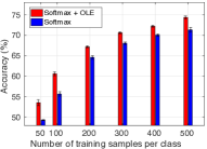
Figure 5: Accuracy versus number of samples. The improved generalization when using OLÉ is more significant when fewer training samples are available. For this experiment we used STL-10 without data augmentation and we average ofer 5 runs.

4.5 Novelty Detection

In this subsection we further analyze the Facescrub-500 experiment and show that the OLÉ loss improves the novelty detection capability of the network. The goal of novelty detection [19, 24] is to identify images in the test set that do not belong to any of the categories in the training set.

Of the 530 identities in the Facescrub dataset, we took 500 identities to form the Facescrub-500 dataset, and we left the remaining 30 identities as the novel classes used to assess novelty detection performance. We use all the images from the novel classes for testing (3,220 in total).

Ideally, since the novel identities are none of the known 500 subjects, their 500 class scores should all be low. We observe that this is the case when using OLÉ, whereas when using only the softmax loss, there is typically one class out of the known 500 that will have a confident softmax score (close to 1), see Fig. 6. To show this, we varied a threshold $t\in[0,1]$ over the softmax scores and defined the False Positive Ratio (FPR), as the number of images of the novel classes whose softmax score is higher than $t$. In Fig. 6(a) we plot the model accuracy in the 500 known subjects against the FPR. When using the OLÉ loss, the model is able to reject most unknown classes without significant loss of accuracy on the known 500. Fig. 6(b) shows the histogram of softmax scores for images of the novel classes when using OLÉ. Most of the scores are concentrated around $1/500$, reflecting the low confidence the OLÉ network gives to the novel classes. On the other hand, the network trained with only the softmax loss gives high confidence scores to images of the novel classes, see Fig. 6(c).

We verified that the OLÉ deep network did not lose face representation power in the novel classes by running the standard verification benchmark on the Labeled Faces in the Wild (LFW) [12]. We observed similar AUC ($99.04\%$ vs $99.12\%$) and verification performance ($96.57\%$ vs $96.64\%$) for the models with and without the OLÉ loss, respectively.

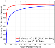
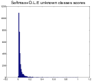
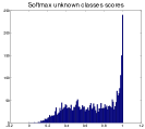
(a)	(b)	(c)

Figure 6: Application to novelty detection. (a) Accuracy on 500 known identities versus ratio of the images of the 30 novel classes that are wrongly classified as one of the known 500, when varying a threshold on the class scores. When using the OLÉ loss, more false positives can be avoided without losing classification performance on the known classes. (b) & (c) Histogram of the maximum class scores for samples from the novel classes, with and without OLÉ, respectively. In (b), scores are concentrated towards $1/500$, whereas in (c), false high confidence scores are generally obtained.

4.6 Visualization of the Obtained Features

We illustrate the geometry of the learned deep features using OLÉ in Fig. 1. In (a) and (b) we show a Barnes-Hut-SNE visualization [32] of the obtained embedding for the validation set of CIFAR10. The intra-class low-rank minimization reduces the intra-class variance to only one dimension. The overall rank maximization produces more margin (orthogonality) between classes.

In Fig. 1 (c) and (d), we show the angle between the deep features of (a) and (b). The 10,000 validation images are ordered by class. With OLÉ, the relative angle is mostly 0 for images of the same class, and 90 for images of different class. On the other hand, for the standard softmax loss, the learned deep features have a larger intra-class spread, and inter-class angles are not always orthogonal.

Finally, we show the spectral decomposition of the deep feature matrices for CIFAR10 validation set in Fig. 7. With OLÉ, the deep features are concentrated along 10 principal dimensions, corresponding to the learned orthogonal linear subspaces. For the softmax loss, the deep feature matrix has its energy distributed along many directions, reflecting the more spreading of the deep features vectors.

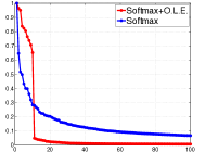
Figure 7: Spectral analysis of the deep feature matrix obtained for CIFAR10 validation data using VGG-16. We plot the normalized singular values of the feature matrix with and without OLÉ. When using OLÉ, the deep features are concentrated along 10 strong dimensions in the embedding space, corresponding to the linear subspaces where the features are compacted. For the standard softmax, the energy is distributed more evenly.

5 Conclusions

We proposed OLÉ, a novel objective function for deep networks that simultaneously encourages intra-class compactness and inter-class separation of the deep features. The former is imposed as a low-rank constraint and the latter as an orthogonalization constraint. The proposed OLÉ loss can be used standalone as a classification loss or in combination with the standard softmax loss for improved performance. We showed that OLÉ produces more discriminative deep networks and deep representations whose energy in the embedding space is concentrated in a few dimensions. For classification, OLÉ is particularly effective when training data is scarce. Using OLÉ, we significantly advance the state-of-the-art classification performance in the standard STL-10 benchmark. The proposed loss introduces a new paradigm to deep metric learning and we believe it will be a valuable tool in applications where orthogonality in the deep representations is required.

References

- [1] De Cheng, Yihong Gong, Sanping Zhou, Jinjun Wang, and Nanning Zheng. Person re-identification by multi-channel parts-based cnn with improved triplet loss function. In Proceedings of the IEEE Conference on Computer Vision and Pattern Recognition, pages 1335–1344, 2016.
- [2] Sumit Chopra, Raia Hadsell, and Yann LeCun. Learning a similarity metric discriminatively, with application to face verification. In Proceedings of the IEEE Conference on Computer Vision and Pattern Recognition, volume 1, pages 539–546. IEEE, 2005.
- [3] Adam Coates, Andrew Ng, and Honglak Lee. An analysis of single-layer networks in unsupervised feature learning. In Proceedings of the fourteenth International Conference on Artificial Intelligence and Statistics, pages 215–223, 2011.
- [4] Xavier Glorot and Yoshua Bengio. Understanding the difficulty of training deep feedforward neural networks. In Proceedings of the Thirteenth International Conference on Artificial Intelligence and Statistics, pages 249–256, 2010.
- [5] Raia Hadsell, Sumit Chopra, and Yann LeCun. Dimensionality reduction by learning an invariant mapping. In Proceedings of the IEEE Conference on Computer Vision and Pattern Recognition, volume 2, pages 1735–1742. IEEE, 2006.
- [6] Kaiming He, Georgia Gkioxari, Piotr Dollár, and Ross Girshick. Mask R-CNN. 2017.
- [7] Kaiming He, Xiangyu Zhang, Shaoqing Ren, and Jian Sun. Delving deep into rectifiers: Surpassing human-level performance on imagenet classification. In Proceedings of the IEEE Conference on Computer Vision and Pattern Recognition, pages 1026–1034, 2015.
- [8] Kaiming He, Xiangyu Zhang, Shaoqing Ren, and Jian Sun. Deep residual learning for image recognition. In Proceedings of the IEEE Conference on Computer Vision and Pattern Recognition, pages 770–778, 2016.
- [9] Kaiming He, Xiangyu Zhang, Shaoqing Ren, and Jian Sun. Identity mappings in deep residual networks. In European Conference on Computer Vision, pages 630–645. Springer, 2016.
- [10] Junlin Hu, Jiwen Lu, and Yap-Peng Tan. Discriminative deep metric learning for face verification in the wild. In Proceedings of the IEEE Conference on Computer Vision and Pattern Recognition, pages 1875–1882, 2014.
- [11] Gao Huang, Zhuang Liu, Kilian Q Weinberger, and Laurens van der Maaten. Densely connected convolutional networks. arXiv preprint arXiv:1608.06993, 2016.
- [12] Gary B Huang, Manu Ramesh, Tamara Berg, and Erik Learned-Miller. Labeled faces in the wild: A database for studying face recognition in unconstrained environments. Technical report, Technical Report 07-49, University of Massachusetts, Amherst, 2007.
- [13] Pan Ji, Tong Zhang, Hongdong Li, Mathieu Salzmann, and Ian Reid. Deep subspace clustering networks. arXiv preprint arXiv:1709.02508, 2017.
- [14] Vahid Kazemi and Josephine Sullivan. One millisecond face alignment with an ensemble of regression trees. In Proceedings of the IEEE Conference on Computer Vision and Pattern Recognition, 2014.
- [15] Alex Krizhevsky and Geoffrey Hinton. Learning multiple layers of features from tiny images. 2009.
- [16] Chen-Yu Lee, Saining Xie, Patrick Gallagher, Zhengyou Zhang, and Zhuowen Tu. Deeply-supervised nets. In Artificial Intelligence and Statistics, pages 562–570, 2015.
- [17] Weiyang Liu, Yandong Wen, Zhiding Yu, Ming Li, Bhiksha Raj, and Le Song. Sphereface: Deep hypersphere embedding for face recognition. arXiv preprint arXiv:1704.08063, 2017.
- [18] Weiyang Liu, Yandong Wen, Zhiding Yu, and Meng Yang. Large-margin softmax loss for convolutional neural networks. In International Conference on Machine Learning, pages 507–516, 2016.
- [19] Amit Mandelbaum and Daphna Weinshall. Distance-based confidence score for neural network classifiers. arXiv preprint arXiv:1709.09844, 2017.
- [20] Yuval Netzer, Tao Wang, Adam Coates, Alessandro Bissacco, Bo Wu, and Andrew Y Ng. Reading digits in natural images with unsupervised feature learning. In NIPS workshop on deep learning and unsupervised feature learning, volume 2011, page 5, 2011.
- [21] Hong-Wei Ng and Stefan Winkler. A data-driven approach to cleaning large face datasets. In Image Processing (ICIP), 2014 IEEE International Conference on, pages 343–347. IEEE, 2014.
- [22] O. M. Parkhi, A. Vedaldi, and A. Zisserman. Deep face recognition. In British Machine Vision Conference, 2015.
- [23] Xi Peng, Jiashi Feng, Shijie Xiao, Jiwen Lu, Zhang Yi, and Shuicheng Yan. Deep sparse subspace clustering. arXiv preprint arXiv:1709.08374, 2017.
- [24] Marco AF Pimentel, David A Clifton, Lei Clifton, and Lionel Tarassenko. A review of novelty detection. Signal Processing, 99:215–249, 2014.
- [25] Qiang Qiu and Guillermo Sapiro. Learning transformations for clustering and classification. Journal of Machine Learning Research, 16(187-225):2, 2015.
- [26] Benjamin Recht, Maryam Fazel, and Pablo A Parrilo. Guaranteed minimum-rank solutions of linear matrix equations via nuclear norm minimization. SIAM review, 52(3):471–501, 2010.
- [27] Oren Rippel, Manohar Paluri, Piotr Dollar, and Lubomir Bourdev. Metric learning with adaptive density discrimination. arXiv preprint arXiv:1511.05939, 2015.
- [28] Florian Schroff, Dmitry Kalenichenko, and James Philbin. Facenet: A unified embedding for face recognition and clustering. In Proceedings of the IEEE Conference on Computer Vision and Pattern Recognition, pages 815–823, 2015.
- [29] Karen Simonyan and Andrew Zisserman. Very deep convolutional networks for large-scale image recognition. arXiv preprint arXiv:1409.1556, 2014.
- [30] Yi Sun, Yuheng Chen, Xiaogang Wang, and Xiaoou Tang. Deep learning face representation by joint identification-verification. In Advances in Neural Information Processing Systems, pages 1988–1996, 2014.
- [31] Martin Thoma. Analysis and optimization of convolutional neural network architectures. arXiv preprint arXiv:1707.09725, 2017.
- [32] Laurens Van Der Maaten. Barnes-Hut-SNE. arXiv preprint arXiv:1301.3342, 2013.
- [33] Rene Vidal, Yi Ma, and Shankar Sastry. Generalized principal component analysis (GPCA). IEEE Transactions on Pattern Analysis and Machine Intelligence, 27(12):1945–1959, 2005.
- [34] G Alistair Watson. Characterization of the subdifferential of some matrix norms. Linear algebra and its applications, 170:33–45, 1992.
- [35] Yandong Wen, Kaipeng Zhang, Zhifeng Li, and Yu Qiao. A discriminative feature learning approach for deep face recognition. In European Conference on Computer Vision, pages 499–515. Springer, 2016.