Majorana bound states in hybrid 2D Josephson junctions with ferromagnetic insulators

Abstract

We consider a Josephson junction consisting of superconductor/ferromagnetic insulator (S/FI) bilayers as electrodes which proximizes a nearby 2D electron gas. By starting from a generic Josephson hybrid planar setup we present an exhaustive analysis of the the interplay between the superconducting and magnetic proximity effects and the conditions under which the structure undergoes transitions to a non-trivial topological phase. We address the 2D bound state problem using a general transfer matrix approach that reduces the problem to an effective 1D Hamiltonian. This allows for straightforward study of topological properties in different symmetry classes. As an example we consider a narrow channel coupled with multiple ferromagnetic superconducting fingers, and discuss how the Majorana bound states can be spatially controlled by tuning the superconducting phases. Following our approach we also show the energy spectrum, the free energy and finally the multiterminal Josephson current of the setup.

Introduction. Majorana bound states (MBS) Kitaev (2001) have been proposed as a building block for solid-state topological quantum computation Kitaev (2003); *Nayak2008. Different setups have been discussed theoretically Fu and Kane (2008); Oreg et al. (2010); *stanescu2010-pea; *stanescu2011; *sau2010-gnp; *Lutchyn2010; Alicea (2010); *Alicea2012; Hell et al. (2017a); *hell2017-cbm; Sticlet et al. (2017); Pientka et al. (2017); Prada et al. (2012); Rainis et al. (2013) — many of them relying on the combination of materials with strong spin-orbit coupling, superconductors and external magnetic field. Following these suggestions, experimental research has been focused on hybrid structures between semiconducting nanowires Mourik et al. (2012) and more recently two-dimensional electron systems Tanaka et al. (2009); Williams et al. (2012); Oostinga et al. (2013); *Sochnikov2015; Kurter et al. (2015); Kjærgaard et al. (2016); Bocquillon et al. (2016); *Wiedenmann2016; Shabani et al. (2016); *zutic2016; Suominen et al. (2017) in proximity to superconducting leads. Setups based on 2DEGs are of special interest, as they benefit from the precise control of the 2DEG quantum well technology developed in the last 40 years. Ideally, the external magnetic field should act as a pure homogeneous Zeeman field acting on the conduction electrodes of the semiconductor. In practice, in the presence of superconductors, the situation is more complex due to orbital effects and spatial inhomogeneity due to magnetic focusing Lee et al. (2013); Paajaste et al. (2015); *tiira2017magnetically; Zuo et al. (2017).

The aim of the present work is twofold: to propose a setup for hosting and manipulating MBS at zero external magnetic field, and to discuss a general analytical approach for describing the transport and topological properties of 1D boundary systems with generic symmetries. The proposed setup is sketched in Fig. 1 which consists of a 2DEGDeon et al. (2011a); *Deontwo11; *Amado13; *Amadotwo2013; *Fornieri13 coupled to ferromagnetic insulator/superconductor (FI/S) electrodes. Related 2D systems have been recently explored in Refs. Pientka et al. (2017); Hell et al. (2017a); Sticlet et al. (2017); Konschelle et al. (2016a); *konschelle2016b. The magnetic proximity effect from the FI induces an effective exchange field $\bm{h}$ in the superconductors breaking time-reversal symmetry and resulting in a spin splitting of the density of states. Experimentally, manufacturing S/FI films is well demonstrated. Moodera et al. (1988); *hao1990spin; Strambini et al. (2017). We approach the theoretical problem by developing an exact method that provides a systematic dimensional reduction procedure based on a continuum transfer matrix approach Lee and Joannopoulos (1981); Hatsugai (1993); Mora et al. (1985); Garcia-Moliner et al. (1990), which in certain aspects is closely related to scattering theory Beenakker and van Houten (1991); *beenakker2015-rmt. The effective 1D boundary Hamiltonian obtained provides access to the energy spectrum, the free energy Gel’fand and Yaglom (1960); Forman (1987); Waxman (1994); Kosztin et al. (1998), and the multiterminal Josephson currents in the setup. An analytically tractable 1D topological invariant also emerges in a natural manner. The approach also applies to 2DEG strongly coupled to superconductors via transparent interfaces, required for large topological energy gaps. Here, we apply this method for our class D problem Ryu et al. (2010); *RMPChiu2016 and discuss phase-controlled manipulation Fu and Kane (2008); Romito et al. (2012) of the MBS with inhomogeneous multiple S/FI ”fingers”.

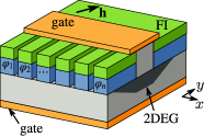
Figure 1: Schematic of a narrow semiconductor channel (2DEG/nanowire) contacted to ferromagnetic insulator–superconductor bilayers. Phase differences $\varphi_{j}$ of the superconducting $j$-th fingers are imposed across the semiconductor channel. Multiple fingers can be used to precisely control the position of the topological bound states in the junction.

Model. To model the junction of Fig. 1 we use the Bogoliubov–de-Gennes Hamiltonian of the proximized 2DEG in the basis $(\psi_{\uparrow},\psi_{\downarrow},-\psi_{\downarrow}^{\dagger},\psi_{\uparrow}^{\dagger})$,

$$\mathcal{H}=\hat{\nabla}\cdot\frac{-\tau_{3}}{2m(x,y)}\hat{\nabla}-\mu(x,y)\tau_{3}-\bm{h}(x,y)\cdot\bm{\sigma}+\hat{\Delta}(x,y)\,.$$ (1)

Here, $\hat{\nabla}=\nabla+i\hat{x}[\bm{\alpha}_{x}(x,y)\cdot\bm{\sigma}]+i\hat{y}[\bm{\alpha}_{y}(x,y)\cdot\bm{\sigma}]=\hat{x}\hat{\partial}_{x}+\hat{y}\hat{\partial}_{y}$ contains the spin-orbit su(2) vector potential. Fröhlich and Studer (1993) The superconducting order parameter is $\hat{\Delta}=\frac{1}{2}[\tau_{1}+i\tau_{2}]\Delta+\frac{1}{2}[\tau_{1}-i\tau_{2}]\Delta^{\dagger}$, $\bm{h}$ is the exchange field, and $m$ the effective mass. Moreover, $\tau_{1,2,3}$ and $\sigma_{x,y,z}$ are Pauli matrices in the Nambu and spin spaces, respectively. We assume that inside the “lead” region, $|y|>L/2$, the parameters are independent of $y$ but may vary along $x$.

Reduction to 1D. To study the Andreev bound states (ABS) localized in the $|y|<L/2$ region, we reduce the problem from 2D to 1D using the transfer matrix Lee and Joannopoulos (1981); Hatsugai (1993); Mora et al. (1985); Garcia-Moliner et al. (1990); Waxman (1994); Titov and Beenakker (2006). Consider first the 2D Schrödinger equation $G^{-1}(\epsilon)\psi=[\epsilon-\mathcal{H}]\psi=0$ and define the vector $\mathbf{u}=(\psi;\tau_{3}(2m)^{-1}\hat{\partial}_{y}\psi)$. $\psi$ satisfies the differential equation when $\partial_{y}\mathbf{u}(y)=\mathbf{W}(y)\mathbf{u}(y)$, where

$$\mathbf{W}(x,y)=\begin{pmatrix}-i\bm{\alpha}_{y}(x,y)\cdot\bm{\sigma}&2m(x,y)\tau_{3}\\ \mathcal{H}\rvert_{\hat{\partial}_{y}=0}-\epsilon&-i\bm{\alpha}_{y}(x,y)\cdot\bm{\sigma}\end{pmatrix}\,.$$ (2)

The fundamental matrix $\mathbf{\Psi}(y,y^{\prime})$, such that $\mathbf{u}(y)=\mathbf{\Psi}(y,y^{\prime})\mathbf{u}(y^{\prime})$, satisfies $\partial_{y}\mathbf{\Psi}(y,y^{\prime})=\mathbf{W}(y)\mathbf{\Psi}(y,y^{\prime})$ with $\mathbf{\Psi}(y,y)=\mathbf{1}$. Below we denote Pauli matrices in the above $2\times 2$ space with $\gamma_{1,2,3}$. Note that $\mathbf{W}$ and $\mathbf{\Psi}$ are operators in $x$-basis, and in a uniform system, $\det[\mathbf{W}(k_{x})-ik_{y}\mathbf{1}]=(2m)^{4}\det[\mathcal{H}(k_{x},k_{y})-\epsilon]$. At the interfaces with the leads, $y=\pm{}L/2$, $\psi$ satisfies boundary conditions of the form $\psi+A_{\pm}\hat{\partial}_{y}\psi=0$. The coefficients $A_{\pm}$ contain information about the FI/S leads and are determined by their $\mathbf{W}$ matrices. The boundary conditions can be expressed as $\mathbf{M}_{y}\mathbf{u}(y)\equiv{}[\mathbf{P}_{-}\mathbf{\Psi}(-L/2,y)+\mathbf{P}_{+}\mathbf{\Psi}(L/2,y)]\mathbf{u}(y)=0$, where

$$\mathbf{P}_{-} =\begin{pmatrix}1&2mA_{-}\tau_{3}\\ 0&0\end{pmatrix}\,, \mathbf{P}_{+} =\begin{pmatrix}0&0\\ (2m)^{-1}\tau_{3}A_{+}^{-1}&1\end{pmatrix}\,.$$ (3)

The bound state energies are then determined by $\operatorname{Det}\mathbf{M}_{y}(\epsilon)=0$ where $\operatorname{Det}$ is the (functional) determinant in the matrix and $x$ spaces. It is independent of $y$ because $\operatorname{Det}\mathbf{\Psi}(y,y^{\prime})=1$. We can characterize the ABS with a 1D boundary/defect Hamiltonian Lee and Joannopoulos (1981); Peng et al. (2017) based on the Green function $G$:

$$H_{y}=\epsilon-L^{-1}G(y,y)^{-1}\,.$$ (4)

The transformation (2) provides an explicit connection between $G$ and $\mathbf{M}_{y}$, typical Kosztin et al. (1998) for such differential equation systems: epa

$$H_{y} =\epsilon-2L^{-1}[\mathbf{M}_{y}^{-1}\gamma_{3}\mathbf{M}_{y}]_{12}^{-1}\,,$$ (5)

$$\operatorname{Det}(\epsilon-H_{y}) =\operatorname{Det}{}(\mathbf{M}_{y})\operatorname{Det}^{-1}([\frac{L}{2}\mathbf{P}_{-}\mathbf{\Psi}_{-}]_{12}[\mathbf{P}_{+}\mathbf{\Psi}_{+}]_{22})\,,$$ (6)

where $\mathbf{\Psi}_{\pm}=\mathbf{\Psi}(\pm\frac{L}{2},y)$ and $[\mathbf{X}]_{12}=\begin{pmatrix}1&0\end{pmatrix}\mathbf{X}\begin{pmatrix}0&1\end{pmatrix}^{T}$, $[\mathbf{X}]_{22}=\begin{pmatrix}0&1\end{pmatrix}\mathbf{X}\begin{pmatrix}0&1\end{pmatrix}^{T}$. Solutions to the eigenproblem $H_{y}(\epsilon)\psi=\epsilon\psi$ give the bound state energies. Zeros of the denominator of Eq. (6) correspond to a bound state in either half of the system cut into two with a hard-wall boundary condition $\psi(y)=0$. If the leads are topologically trivial so that the edge of the cut system is gapped, $H_{y}$ is typically nonsingular at low energies.

Topological order. Hamiltonian (1) has the charge-conjugation symmetry $\mathcal{H}=-C^{\dagger}\mathcal{H}^{*}C$, $C=-\sigma_{y}\tau_{y}$. As $H_{y}$ inherits the symmetry of $\mathcal{H}$, its topological properties can be characterized by the low-energy part of the 1D bulk invariant of class D: Kitaev (2001)

$$\chi(y)=-\mathop{\mathrm{sgn}}\mathop{\mathrm{pf}}{}CH_{y}(\epsilon=0,k_{x}=0)\,,$$ (7)

where $\mathop{\mathrm{pf}}$ is the Pfaffian of a $4\times 4$ matrix. Note that $\chi(y)$ can change sign only if bound states cross $\epsilon=0$, or when $H_{y}$ has a singularity there. As a consequence, zero-energy bound states are expected between regions with different $\chi$. This argument can be generalized to other symmetry classes and formally also to 0D invariants in systems of finite size along $x$.

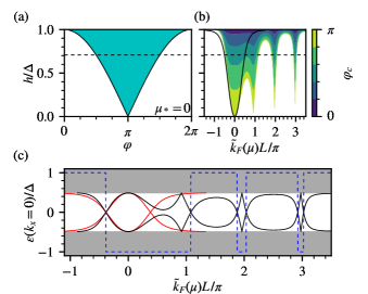
Figure 2: Topological phase diagram. (a) The quantity $\chi(y=0)$ (shaded: $-1$) and the 1D narrow-channel invariant $\mathcal{M}$ (solid line: sign change), for $\bm{\alpha}_{x}\perp\bm{h}$, $\bm{\alpha}_{y}=0$. Dotted line indicates the Chandrasekhar–Clogston limit $h=\Delta/\sqrt{2}$. (b) Threshold $\varphi_{c}$, such that $\chi=-1$ for $\varphi_{c}<\varphi<2\pi-\varphi_{c}$, for varying $\mu$. Here, $\tilde{k}_{F}(\mu)\equiv\sqrt{2m|\mu_{*}|}\mathop{\mathrm{sgn}}\mu_{*}$. The threshold for nontrivial state at $\varphi=\pi$ in the narrow-channel 1D model is also shown (solid line). (c) Mode spectrum at $k_{x}=0$, exact (solid black) and from $\mathcal{H}_{\rm eff}$ (solid red), and $\chi$ (dashed), for $h/\Delta=0.5$, $\varphi=\pi$. We set $k_{S}=5/\xi$, $\bm{\alpha}_{x}=\hat{x}0.5/\xi$, $\bm{\alpha}_{y}=0$, $L=0.25\xi$, $k_{x}=0$, and $\xi=\hbar/\sqrt{2m|\Delta|}$.

Infinite superconducting leads. For this specific case, we determine the $A_{\pm}$ factors from the $\mathbf{W}$ matrices in the leads, $\mathbf{W}_{\pm}$. We define the projectors $\tilde{\mathbf{P}}_{+(-)}=\frac{1+(-)\mathop{\mathrm{sgn}}{}\mathbf{W}_{+(-)}}{2}$ to growing(decreasing) modes with momenta $+(-)\mathop{\mathrm{Im}}{}k_{y}<0$ in the upper(lower) lead, where $\mathop{\mathrm{sgn}}$ is the matrix sign function. The mode matching conditions for bound states can then be written as $\tilde{\mathbf{P}}_{\pm}\mathbf{u}(\pm{}L/2)=0$. At energies where the spectrum of the leads is gapped, half of the modes are growing and half are decreasing. Since $\tilde{\mathbf{P}}_{\pm}$ are then half-rank matrices, one can generally find $\mathbf{R}$ such that $\tilde{\mathbf{P}}_{\pm}=\mathbf{R}\mathbf{P}_{\pm}$ where $\mathbf{P}_{\pm}$ have the structure of Eq. (3). For $\mu_{\rm lead}\to\infty$ and no spin-orbit interaction in the leads, direct calculation gives epa $A_{\pm}=\mp\frac{1}{ik_{S}}\tau_{3}g\tau_{3}$, where $g$ is the quasiclassical Eilenberger (1968) Green function $g=[(\epsilon-\bm{h}\cdot\bm{\sigma})\tau_{3}+\Delta\tau_{1}]/\sqrt{(\epsilon-\bm{h}\cdot\bm{\sigma})^{2}-|\Delta|^{2}}$ and $k_{S}=\frac{m}{m_{\rm lead}}\sqrt{2m_{\rm lead}\mu_{\rm lead}}$ a mismatch parameter.

Narrow-channel expansion. Consider now a narrow channel with a Hamiltonian constant on $|y|<L/2$. Then $\mathbf{\Psi}(y,y^{\prime})=e^{(y-y^{\prime})\mathbf{W}}$. Expanding to leading orders in $L$ ($\lesssim{}[2m(|\mu|+|\epsilon|)]^{-1/2}$) in Eq. (5) we obtain

$$\begin{split}\mathcal{H}_{\rm eff}&=H_{y=0}=\mathcal{H}\rvert_{\hat{\partial}_{y}=0}+\Sigma\,,\\ \Sigma&=-\frac{\tau_{3}}{2mL}(A_{-}^{-1}-A_{+}^{-1})-\frac{\tau_{3}}{4m}(A_{-}^{-2}+A_{+}^{-2})\\ &\quad+\frac{\tau_{3}}{4m}[A_{-}^{-1}+A_{+}^{-1},-i\bm{\alpha}_{y}\cdot\bm{\sigma}]+\mathcal{O}(L^{1})\,.\end{split}$$ (8)

When $\bm{\alpha}_{y}$ is parallel to the exchange field of the leads, it commutes with $A_{\pm}$ and does not contribute. Imperfections in the S/N interfaces may also be included in this model and will affect the precise form of $A_{\pm}$. The above Hamiltonian is obtained via operator manipulations, and we did not need to e.g. select a variational wave function basis.

Within the quasiclassical limit in the leads and by setting for simplicity $\bm{\alpha}_{y}\parallel\bm{h}$ , Eq. (8) can be written as

$$\mathcal{H}_{\rm eff}(\epsilon) =\Bigl{[}-\frac{1}{2m}(\partial_{x}+i\bm{\alpha}_{x}\cdot\bm{\sigma})^{2}-\mu+\frac{k_{S}^{2}}{2m}\Bigr{]}\tau_{3}$$ (9)

$$\quad-\bm{h}_{*}(\epsilon)\cdot\bm{\sigma}+\hat{\Delta}_{*}(\epsilon)-(Z_{*}^{-1}(\epsilon)-1)\epsilon\,$$

yielding an effective 1D Hamiltonian with an energy dependent order parameter $\hat{\Delta}_{*}$, an exchange field $\bm{h}_{*}$, a potential shift, and an energy renormalization [see Eqs. (S6) in epa for explicit expressions]. We have neglected the $k_{x}$ dependence of $A_{\pm}$, by assuming $k_{x}\ll{}k_{F,\mathrm{lead}}$. For leads with identical $|\Delta|$, $|\bm{h}|$ and phase difference $\varphi$, we find at $\epsilon\to 0$, $Z_{*}^{-1}=1+D_{*}|\Delta|^{2}/(|\Delta|^{2}-|\bm{h}|^{2})$ and $\Delta_{*}=D_{*}|\Delta|\cos\frac{\varphi}{2}$, $\bm{h}_{*}=D_{*}\bm{h}$, where $D_{*}=2\hbar^{2}k_{S}/[2mL\sqrt{\Delta^{2}-|\bm{h}|^{2}}]$. At low energies, Eq. (9) is similar to widely studied quantum wire models Oreg et al. (2010); Stanescu et al. (2010), and characterized by the same 1D topological invariant in class D Kitaev (2001) $\mathcal{M}=\mathop{\mathrm{sgn}}\mathop{\mathrm{pf}}C\mathcal{H}_{\rm eff}(k_{x}=0)\mathop{\mathrm{pf}}C\mathcal{H}_{\rm eff}(k_{x}=\infty)$.

The superconducting self-energy in Eq. (9) in the limit considered here ($L\to 0$, transparent NS interfaces) turns out to be similar in form to weak-coupling tunneling models, Stanescu et al. (2010); Sau et al. (2010); Alicea (2010); Sau et al. (2011); Stanescu and Tewari (2013) derived projecting onto lowest quantum well confined modes in the N-region. The explicit expressions for the prefactors, the shift in the potential, and $\alpha_{y}$ spin-orbit obtained here are not found in typical tunneling approaches. The magnetic proximity effect from ferromagnetic superconductors that affects the energy dependence of both the superconducting and exchange self-energies, on the other hand in principle can be captured also by a tunneling calculation.

Phase diagram and spectrum. Figure 2(a) shows $\chi$ and the 1D invariant $\mathcal{M}=\mathop{\mathrm{sgn}}[\mu_{*}^{2}+|\Delta_{*}|^{2}-h_{*}^{2}]$, where $\mu_{*}=\mu-\frac{k_{S}^{2}+\alpha_{x}^{2}}{2m}$, for a class D narrow Josephson junction, translationally invariant along $x$, under a phase difference $\varphi$. This is in agreement with the phase diagram presented in Ref. Pientka et al., 2017, for the specific value of $\mu_{*}$. The chemical potential dependence is shown in Fig. 2(b), together with the size of the $\chi=-1$ region around $\varphi=\pi$. The behavior as a function of $\mu$ with constant $k_{S}$ exhibits finite-size $k_{F}L$ oscillations from scattering at the NS interface, which are not present Sticlet et al. (2017); Pientka et al. (2017) in the result (not shown) for the matched case $\mu=\mu_{\mathrm{lead}}$, $m=m_{\mathrm{lead}}$ where $\mu_{*}=\mathrm{const}(\mu)$. The correspondence between $\chi$ and the mode spectrum at $k_{x}=0$ is shown in Fig. 2(c). The above narrow-channel approximation breaks down when $|k_{F}|L\gtrsim 1$, and is applicable for the first lobe. This limitation is also visible in Fig. 2(c), where the narrow-channel approximation predicts a zero-energy crossing between $0<\tilde{k}_{F}L<\pi$, whereas in the exact solution the system is in the nontrivial state for the whole interval. Nevertheless, states with $\chi=-1$ can be achieved also at higher doping and mismatch, but in a narrower parameter region.

It is important to note that S/FI bilayers have restrictions on the magnitude of the exchange field. The S/FI bilayer energy spectrum becomes gapless at $h>\Delta$. Moreover, thin S/FI bilayers at low temperatures support a thermodynamically stable superconducting state only below the limit $h<\Delta(T=0)/\sqrt{2}$ Clogston (1962); Chandrasekhar (1962); Maki and Tsuneto (1964) above which a first-order transition to normal state occurs at $T=0$. As the induced effective order parameter is $\Delta_{*}\propto|\cos\frac{\varphi}{2}|$, a change of the 1D invariant can however be achieved for any $h$ at phase differences close enough to $\varphi=\pi$.

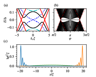
Figure 3: (a) Mode dispersion in the trivial state $\varphi=0.6\pi$ (dash-dotted), at gap closing $\varphi=\varphi_{c}=0.704\pi$ (dotted), non-trivial state $\varphi=0.8\pi$ (black), and second gap closing $\varphi=\pi$ (red). Here $\mu=15\Delta$ and other parameters are as in Fig. 2. (b) Bound state spectrum as a function of $\varphi=\varphi_{j}$ for system size $\ell=40\xi$. The $E_{g}(k_{x}=0)$ bulk gap (10) is also shown (red dashed). (c) Bound state wave function probability densities for $\varphi=0.8\pi$. Shown is the $E\approx 0$ MBS (localized at the ends), and the lowest-energy extended state.

The propagating mode spectrum of the 1D narrow-channel model is shown in Fig. 3(a) for different values of the phase difference. The behavior is typical to quantum wires Kitaev (2001); Oreg et al. (2010): the magnetic and superconducting proximity effects open energy gaps at $k_{x}=0$ and $k_{x}=k_{F}$. The energy gap at $k_{x}=0$

$$E_{g}(k_{x}=0)\simeq{}Z_{*}\Big{|}|\bm{h}_{*}|-\sqrt{|\Delta_{*}|^{2}+\mu_{*}^{2}}\Big{|}\,,$$ (10)

closes and reopens at the topological transition. The gap at $k_{F}$ closes at $\varphi=\pi$ where $\Delta_{*}$ vanishes.

Finite size. The bound state energies of a system with finite size in the $x$-direction are given by the zeros of the determinant of the effective 1D model, Gel’fand and Yaglom (1960); Forman (1987); Waxman (1994)

$$w(\epsilon)=\operatorname{Det}[\epsilon-\mathcal{H}_{\rm eff}(\epsilon)]=\det\Bigl{[}\begin{pmatrix}1&0\\ 0&0\end{pmatrix}+\begin{pmatrix}0&0\\ 1&0\end{pmatrix}\Psi(\epsilon)\Bigr{]}\,.$$ (11)

Here $\Psi(\epsilon)$ is the fundamental matrix connecting the ends of the 1D channel, for the 1D differential operator $\mathcal{H}_{\rm eff}$, defined analogously to Eq. (2) above. Roots $w(\epsilon_{j})=0$ of the above $8\times 8$ determinant can be found numerically. The bound state wave functions associated with each can be found from the corresponding singular vectors.

Figure 3(b) shows the bound state energy spectrum as a function of the phase difference $\varphi$. When the phase difference crosses the bulk topological transition point, one of the ABS crosses over to form a MBS pinned at $\epsilon\approx 0$ and localized at the ends of the 1D channel [see Fig. 3(c)].

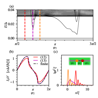
Figure 4: (a) Bound-state spectrum in a finite-size “3-finger” setup with finger widths $\ell_{j}=100\xi,4\xi,100\xi$ and phases $\varphi_{j}=0,\varphi_{2},0.8\pi$, (b) Current density–phase relations, at $T=10^{-3}\Delta$. Shown is the result for uniform junction [Eq. (12)], the same within the narrow-channel approximation [Eq. (13)], and $I_{S,2}/\ell_{2}$ in the 3-finger system. Parameters as in Fig. 3. (c) Sweeping the phase $\varphi_{2}=0.6\pi\mapsto 0.704\pi\mapsto 0.8\pi$, the $\epsilon\approx 0$ MBS localized at $x=\ell_{2}$ (red) moves toward $x=0$ (orange). Other parameters defined in caption of Fig. 2. Inset: schematic of the structure considered.

Supercurrent in a multiple-finger setup. Consider now the geometry of Fig. 1 with multiple superconducting fingers with widths $\ell_{j}$ and different order parameter phases $\varphi_{j}$ on one side. For a spatially piecewise constant Hamiltonian, we then have $\Psi(\epsilon)=\prod_{j}e^{W_{j}(\epsilon,\varphi_{j})\ell_{j}}$. Supercurrent exiting the $j$th superconducting finger is given by the corresponding derivative of the grand potential, which has a closed-form expression:

$$I_{S,j} =\frac{2e}{\hbar}T\partial_{\varphi_{j}}\ln\operatorname{tr}{}e^{-\beta H}=-\frac{e}{\hbar}T\sum_{\omega_{n}}\partial_{\varphi_{j}}\ln\operatorname{Det}\mathbf{M}(i\omega_{n})$$ (12)

$$\simeq-\frac{e}{\hbar}T\sum_{\omega_{n}}\partial_{\varphi_{j}}\ln w(i\omega_{n})\,.$$ (13)

The sum runs over the Matsubara frequencies $\omega_{n}=2\pi{}T(n+\frac{1}{2})$. Here, we used the fact that starting from a functional determinant approach Gel’fand and Yaglom (1960); Forman (1987), $\operatorname{Det}[i\omega-\mathcal{H}]\propto\operatorname{Det}\mathbf{M}(i\omega)\propto\operatorname{Det}[i\omega-\mathcal{H}_{\rm eff}]\propto{}w(i\omega)$, with overall proportionality constants independent epa of $\varphi_{j}$. Resulting current-phase relations are shown in Fig. 4(b), for infinite-length channels ($\ln\operatorname{Det}\mapsto\sum_{k_{x}}\ln\det$) and for a finite-length $\ell<\infty$ system. The results from (12) and (13) differ somewhat at $L=0.25\xi$, but approach each other as the channel width $L\to 0$. The finite-size system result is close to the infinite-size result.

Phase control of the MBS. Consider now a superconducting finger of width $\ell_{2}$ between a trivial ($\varphi_{1}=0$, $x<0$) and a nontrivial ($x>\ell_{2}$, $\varphi_{3}=0.8\pi$) segment. The bound state spectrum as a function of $\varphi_{2}$ is shown in Fig. 4(a). As $\varphi_{2}$ crosses the bulk transition point $\varphi_{c}\approx 0.7\pi$ of the segment, the MBS initially localized at $x=\ell_{2}$ re-localizes to $x=0$ (see Fig. 4(c)). We have assumed $\ell_{2}\sim\xi$ so that the energy gap remains large also when sweeping the phase. The result shows that in a multi-finger setup, the MBS location can be controlled, envisioning 2D channel networks with FI/S electrodes as a platform for a phase-controlled braiding of the MBS. Fu and Kane (2008); Hell et al. (2017b) To drive a segment into the non-trivial state ($\varphi\to\pi$) one can use a superconducting loop, connected to at least to some of the fingers. By controlling the supercurrent, it is likely possible to fine tune the MBS position.

InAs-2DEGDeon et al. (2011a); *Deontwo11; *Amado13; *Amadotwo2013; *Fornieri13 with Al/EuS leadsMoodera et al. (1988); Hao et al. (1990); Strambini et al. (2017) provide a topological gap of $E_{g}/k_{B}\gtrsim 60\,\mathrm{mK}$. The corresponding coherence length is $\xi\sim 80\,\mathrm{nm}$, making the fabrication of the devices compatible with the modern technologies. Phase biasing can be implemented with superconducting loops and, in combination with current injection, can be used to fine tune the MBS position.

Conclusions. In summary, we have used a transfer matrix approach to obtain an effective 1D boundary Hamiltonian. We have applied it to compute the spectrum of a S/FI–2DEG junction and to show how the topological properties of the structure can be tuned by the superconducting phase differences and the electrostatic gating. This enables the spatial control of the MBS, and 2D topological networks for braiding operations without requiring strong external magnetic fields. Our approach is quite general, not limited to any specific model or symmetry class, and can be extended to other 1D channel problems with continuum Hamiltonians that are polynomials in $k_{y}$. Moreover, the model can be applied to investigate the properties of Josephson junctions in two and three-dimensional systems, for example surfaces of topological insulators Fu and Kane (2008); Kurter et al. (2015); Amet et al. (2016), or graphene Titov and Beenakker (2006) junctions.

Appendix A Intermediate steps taken

As explained in the main text, we apply a scattering method closely related to mode matching approaches Lee and Joannopoulos (1981); Hatsugai (1993); Mora et al. (1985); Garcia-Moliner et al. (1990) and to computing functional determinants Gel’fand and Yaglom (1960); Forman (1987); Waxman (1994); Kosztin et al. (1998).

Bound state equation.

Let us point out the status of the bound state equation. The result of Refs. Forman (1987) can be written as (note that $\operatorname{tr}\mathbf{W}=0$ and $\det\mathbf{\Psi}=1$),

$$\operatorname{Det}G^{-1}(\epsilon)=\det\bigl{[}\mathbf{p}_{-}+\mathbf{p}_{+}\mathbf{\Psi}(L/2,-L/2)\bigr{]}\,,\quad\mathbf{p}_{-}=\begin{pmatrix}1&0\\ 0&0\end{pmatrix}e^{-\mathbf{W}_{-}L_{-}}\,,\quad\mathbf{p}_{+}=\begin{pmatrix}0&0\\ 1&0\end{pmatrix}e^{\mathbf{W}_{+}L_{+}}\,,$$ (S1)

where $L_{\pm}$ are the lengths of the upper$(+)$ and lower$(-)$ superconducting leads and $L$ that of the normal channel in between. The multiplicative normalization of $\operatorname{Det}$ depends on the highest-order derivative term in $\mathcal{H}$.

Consider the diagonalization $\mathbf{W}_{\pm}=\mathbf{\Phi}_{\pm}\operatorname{diag}(\Lambda_{\pm}^{<},\Lambda_{\pm}^{>})\mathbf{\Phi}_{\pm}^{-1}$ with growing $(\mathop{\mathrm{Re}}\Lambda_{\pm}^{>}>0)$ and decaying $(\mathop{\mathrm{Re}}\Lambda_{\pm}^{<}<0)$ modes, and write $\mathbf{\Phi}=\begin{pmatrix}\phi^{<}&\phi^{>}\\ w^{<}\phi^{<}&w^{>}\phi^{>}\end{pmatrix}$. For $L_{\pm}\to\infty$ and neglecting modes in the leads that decay when moving away from the N-region, $\mathbf{p}_{\pm}\to\mathbf{R}\mathbf{P}_{\pm}$ where $\mathbf{P}_{-}=\begin{pmatrix}1&-[w_{-}^{>}]^{-1}\\ 0&0\end{pmatrix}$, $\mathbf{P}_{+}=\begin{pmatrix}0&0\\ -w_{+}^{<}&1\end{pmatrix}$ are the projection matrices in Eq. (3) of the main text, and $\mathbf{R}=\operatorname{diag}(R_{-},R_{+})$, $R_{-}=\phi^{<}_{-}{}e^{-\Lambda_{-}^{<}{}L_{-}}(\phi_{-}^{<})^{-1}[1-(w_{-}^{>})^{-1}w_{-}^{<}]^{-1}$, $R_{+}=\phi^{>}_{+}{}e^{\Lambda_{+}^{>}{}L_{+}}(\phi_{+}^{>})^{-1}[1-(w_{+}^{<})^{-1}w_{+}^{>}]^{-1}(-w_{+}^{<})^{-1}$, depends only on the lead Hamiltonians. As a consequence, $\operatorname{Det}G^{-1}(\epsilon)\simeq\operatorname{Det}{}R_{+}\operatorname{Det}{}R_{-}\operatorname{Det}\mathbf{M}_{y}$, where $\operatorname{Det}{}R_{\pm}$ are independent of the phase of the order parameter.

Singular vectors.

Each zero $\epsilon_{j}$ of the determinant is associated with one or more singular vectors such that $[\mathbf{P}_{-}+\mathbf{P}_{+}\Psi(L/2,-L/2)]\mathbf{u}_{j}=0$. Each corresponds to a bound state wave function vector $\mathbf{u}(x)=\Psi(x,-L/2)\mathbf{u}_{j}$.

Green function.

The Green function of the original Hamiltonian at $|y|,|y^{\prime}|<L/2$ can be expressed as

$$G(y,y^{\prime})=\begin{pmatrix}1&0\end{pmatrix}\mathbf{\Psi}(y,y_{0})[\mathbf{C}_{+}\theta(y-y^{\prime})-\mathbf{C}_{-}\theta(y^{\prime}-y)]\mathbf{\Psi}(y_{0},y^{\prime})\begin{pmatrix}0&1\end{pmatrix}^{T}\,.$$ (S2)

The constants $\mathbf{C}_{\pm}$ such that $\mathbf{C}_{+}+\mathbf{C}_{-}=\mathbf{1}$ are determined by boundary conditions, and $y_{0}$ is an arbitrary fixed value. Direct calculation shows Eq. (S2) then satisfies $[\epsilon-\mathcal{H}]G(y,y^{\prime})=\mathbf{1}\delta(y-y^{\prime})$. Matching to boundary conditions $\psi+A_{\pm}\hat{\partial}_{y}\psi=0$ and setting $y_{0}=-L/2$, we have $\mathbf{C}_{+}=\mathbf{M}_{y_{0}}^{-1}\mathbf{P}_{-}$, $\mathbf{C}_{-}=\mathbf{M}_{y_{0}}^{-1}\mathbf{P}_{+}\mathbf{\Psi}(L/2,-L/2)$.

Local propagator.

The diagonal resolvent is $G(y,y)=\frac{1}{2}[G(y,y+0^{+})+G(y+0^{+},y)]=\frac{1}{2}\begin{pmatrix}1&0\end{pmatrix}\mathbf{q}(y)\begin{pmatrix}0&1\end{pmatrix}^{T}$. From Eq. (S2) and $\mathbf{C}_{+}-\mathbf{C}_{-}=\mathbf{M}_{y_{0}}^{-1}\gamma_{3}\mathbf{M}_{y_{0}}$ we obtain Eq. (5) in the main text. Eq. (6) follows after block matrix algebra:

$$\mathbf{P}_{-}\mathbf{\Psi}(-\frac{L}{2},y)=\begin{pmatrix}p&q\\ 0&0\end{pmatrix}\,,\quad\mathbf{P}_{+}\mathbf{\Psi}(\frac{L}{2},y)=\begin{pmatrix}0&0\\ r&s\end{pmatrix}\,,\quad G(y,y)^{-1}=q^{-1}p-s^{-1}r\,.$$ (S3)

Free energy.

The free energy can be expressed up to a constant as $\mathcal{F}=-\frac{1}{2}T\sum_{\omega_{n}}\ln\operatorname{Det}{}G^{-1}(i\omega_{n})$. Since $\det{}\mathbf{R}$ and the normalization of $\operatorname{Det}$ are independent of the order parameter phases, $\mathcal{F}(\varphi)=-\frac{1}{2}T\sum_{\omega_{n}}\ln\operatorname{Det}{\mathbf{M}}(i\omega_{n},\varphi)+\mathcal{F}_{0}$. As a consequence, supercurrents $I=\frac{2e}{\hbar}\partial_{\varphi}\mathcal{F}$ flowing in the structure are determined only by $\ln\operatorname{Det}\mathbf{M}$, and by extension, the phase-dependent part of its narrow-channel 1D approximation, $\mathcal{F}(\varphi)\simeq-\frac{1}{2}T\sum_{\omega_{n}}\ln\operatorname{Det}[\mathcal{H}_{\rm eff}-\epsilon]+\mathcal{F}_{0}^{\prime}$.

Supercurrent.

Note also that if restricting Eq. (13) of the main text to low energies, and diagonalizing $\mathcal{H}_{\rm eff}$ yields a well-known result for the supercurrent $I_{S,j}=-\frac{e}{2\hbar}\sum_{m}\tanh\bigl{(}\frac{\epsilon_{m}}{2T}\bigr{)}\partial_{\varphi_{j}}{\epsilon_{m}}$ where $\epsilon_{m}$ are the bound state energies.

Quasiclassical approximation.

In the limit $\mu_{\rm lead}\to\infty$ and $\bm{\alpha}_{x/y}=0$ we can compute the projectors $\tilde{\mathbf{P}}_{\pm}$. Using an integral representation of the matrix sign function, we have

$$\tilde{\mathbf{P}}_{\pm}=\int_{C_{\mp}}\frac{\mathrm{d}k_{y}\,}{2\pi}\frac{1}{ik_{y}\mathbf{1}-\mathbf{W}_{\pm}(k_{x})}=\int_{C_{\mp}}\frac{\mathrm{d}k_{y}\,}{2\pi}\begin{pmatrix}ik_{y}G(k_{x},k_{y})b&G(k_{x},k_{y})\\ -k_{y}^{2}bG(k_{x},k_{y})b&ik_{y}bG(k_{x},k_{y})\end{pmatrix}\,,$$ (S4)

where $b=\frac{\tau_{3}}{2m}$, and $C_{+(-)}$ are counter-clockwise semicircles enclosing the upper(lower) complex half-plane. Poles indicating propagating modes are displaced from the real axis by $\mathop{\mathrm{Im}}\epsilon\neq 0$. Moreover, $G(k_{x},k_{y})=[\epsilon-\mathcal{H}_{\rm lead}(k_{x},k_{y})]^{-1}$ is the Green function. Changing the integration variable to $\xi=\frac{k^{2}}{2m_{\mathrm{lead}}}-\mu_{\mathrm{lead}}$ and taking the limit $\mu_{\mathrm{lead}}\to\infty$ we find

$$\tilde{\mathbf{P}}_{\pm}=\begin{pmatrix}\frac{1}{2}&\mp\frac{im_{\mathrm{lead}}}{k_{F,\mathrm{lead}}}\tau_{3}g_{\pm}\\ \pm{}\frac{ik_{F,\mathrm{lead}}}{4m_{\mathrm{lead}}}g_{\pm}\tau_{3}&\frac{1}{2}\end{pmatrix}\,,$$ (S5)

where $g_{+(-)}=\frac{i}{\pi}\fint_{-\infty}^{\infty}\mathrm{d}\xi\,\tau_{3}G_{\mathrm{upper(lower)}}(\xi)$ are the quasiclassical functions in the leads, with $\fint_{-\infty}^{\infty}\equiv\frac{1}{2}\int_{C_{+}}-\frac{1}{2}\int_{C_{-}}$. Since $g_{\pm}^{2}=1$, reflecting the half-rank property of the projector $\tilde{\mathbf{P}}_{\pm}$, the first and second rows of $\tilde{\mathbf{P}}_{\pm}\mathbf{u}=0$ are the same equation. Reduction to the form discussed in the main text is then obtained by $\tilde{\mathbf{P}}_{\pm}=\begin{pmatrix}\frac{1}{2}&mA_{+}\tau_{3}\\ \frac{1}{4m}\tau_{3}A_{-}^{-1}&\frac{1}{2}\end{pmatrix}\mathbf{P}_{\pm}$.

Explicit quantum wire model.

The order parameter $\hat{\Delta}_{*}$, the effective exchange field $\bm{h}_{*}$, and the renormalization $Z_{*}$ read explicitly ($j=\mathrm{upper},\mathrm{lower}$)

$$M_{j,\pm} =\frac{D_{j}}{\sqrt{|\Delta_{j}|^{2}-(h_{j}\mp\epsilon)^{2}}}\,,\qquad\hat{\Delta}_{*}=\frac{1}{2}\sum_{j,\pm}M_{j,\pm}[1\pm\frac{\bm{h}_{j}}{h_{j}}\cdot\bm{\sigma}][\Delta_{j}\tau_{+}+\Delta_{j}^{*}\tau_{-}]\,,$$ (S6a)

$$\bm{h}_{*} =\sum_{j,\pm}M_{j,\pm}\frac{h_{j}\mp\epsilon}{2h_{j}}\bm{h}_{j}\,,\qquad Z_{*}^{-1}=1+\sum_{j,\pm}M_{j,\pm}\frac{\epsilon\mp h_{j}}{2\epsilon}\,.$$ (S6b)

Here, $D_{j}=\frac{\hbar^{2}k_{S}}{2mL}$ describes the effective strength of the the coupling to the S leads, and $h_{j}=|\bm{h}_{j}|$. The superconducting proximity effect in the presence of the exchange field also induces an odd-frequency triplet component in the pairing amplitude Bergeret et al. (2005). It is not important for the main physics here as the triplet component vanishes at $\epsilon\to 0$.

A matrix identity.

For piecewise constant Hamiltonians with fundamental matrix $\Psi=\prod_{j=1}^{n}\Psi_{j}$, one has $\det[M+N\Psi]=\det[M+N\Psi_{n}\cdots\Psi_{1}]$, $\Psi_{j}=\Phi_{j}e^{iK_{j}(x_{j+1}-x_{j})}\Phi_{j}^{-1}$ where $K_{j}=\operatorname{diag}(k_{j,1},\ldots,k_{j,m})$. For large $|\mathop{\mathrm{Im}}{}K||x_{j+1}-x_{j}|$, the matrix product is numerically unstable to evaluate. The following identity can be used to improve the conditioning:

$$\det[M+N\Psi_{n}\ldots\Psi_{1}]=\frac{\det B}{\prod_{j}\det\Phi_{j}}\exp(\sum_{j}\operatorname{tr}Q_{j})\,,$$ (S7)

$$B\equiv\begin{pmatrix}M\Phi_{1}(x_{1})&&&&N\Phi_{n}(x_{n+1})\\ -\Phi_{1}(x_{2})&\Phi_{2}(x_{2})&&&\\ &-\Phi_{2}(x_{3})&\Phi_{3}(x_{3})&&\\ &&\ddots&\ddots&\\ &&&-\Phi_{n-1}(x_{n})&\Phi_{n}(x_{n})\end{pmatrix}\,,$$ (S8)

where $\Phi_{j}(x)=\Phi_{j}e^{iK_{j}(x-x_{j})-Q_{j}}$ and $Q_{j}=\operatorname{diag}(q_{j,1},\ldots,q_{j,m})$ such that

$$q_{j,p}=\begin{cases}0\,,&\text{for $\mathop{\mathrm{Im}}k_{j,p}\geq 0$,}\\ -(x_{j+1}-x_{j})\mathop{\mathrm{Im}}k_{j,p}\,,&\text{for $\mathop{\mathrm{Im}}k_{j,p}<0$.}\\ \end{cases}\,.$$ (S9)

The matrix $B$ is typically better conditioned and its log-det can be evaluated via standard methods. Note that $B$ explicitly encodes the boundary and wave function matching conditions.

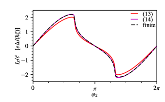
Figure S1: Same as Fig. 4(b), but for $L=0.1\xi$.