Asymptotics to all orders of the Hurwitz zeta function

Abstract

We present several formulae for the large-$t$ asymptotics of the modified Hurwitz zeta function $\zeta_{1}(x,s),x>0,s=\sigma+it,0<\sigma\leq 1,t>0,$ which are valid to all orders. In the case of $x=0$, these formulae reduce to the asymptotic expressions recently obtained for the Riemann zeta function, which include the classical results of Siegel as a particular case.

1 Introduction

The Hurwitz zeta function $\zeta(x,s)$ is a two-variable generalisation of the Riemann zeta function, defined by

$$\zeta(x,s)\coloneqq\sum_{n=0}^{\infty}(n+x)^{-s}\;,\;\;\mathrm{Re}(x)>0,s=\sigma+it,\sigma>1,t\in\mathbb{R},$$

and defined for all $s\in\mathbb{C}$ by analytic continuation. The modified Hurwitz zeta function $\zeta_{1}(x,s)$ is a variant of the Hurwitz zeta function, defined by

$$\zeta_{1}(x,s)\coloneqq\sum_{n=1}^{\infty}(n+x)^{-s}\;,\;\;\mathrm{Re}(x)>-1,s=\sigma+it,\sigma>1,t\in\mathbb{R},$$

and again defined for all $s\in\mathbb{C}$ by analytic continuation. It is clear that these two functions are related by the simple formula

$$\zeta(x,s)=\frac{1}{x^{s}}+\zeta_{1}(x,s)\;,\;\;\mathrm{Re}(x)>0,s\in\mathbb{C},$$

and that for $x=0$ the modified Hurwitz function reduces to the Riemann zeta function:

$$\zeta(s)=\zeta_{1}(x,s).$$

The following asymptotic formula for $\zeta(s)$, proved in e.g. Theorem 4.15 of [10], is known as the approximate functional equation:

$$\zeta(s)=\sum_{n\leq x}\frac{1}{n^{s}}+\chi(s)\sum_{n\leq y}\frac{1}{n^{1-s}}+O\Big{(}x^{-\sigma}+|t|^{\tfrac{1}{2}-\sigma}y^{\sigma-1}\Big{)},$$ (1.1)

where

$$xy=\tfrac{t}{2\pi},0<\sigma<1,t\rightarrow\infty,$$

and the entire function $\chi(s)$ is defined by

$$\chi(s)\coloneqq\tfrac{(2\pi)^{s}}{\pi}\Gamma(1-s)\sin\big{(}\tfrac{\pi s}{2}\big{)},\;s\in\mathbb{C}.$$ (1.2)

(Throughout this paper, $\Gamma(s)$ denotes the gamma function of a complex variable $s$ and $\lfloor k\rfloor$ denotes the floor function of a real number $k$.)

The analogous formula for the modified Hurwitz function is the following asymptotic expression, proved in e.g. [8]:

$$\zeta_{1}(\alpha,s)=\sum_{n=1}^{\lfloor x-\alpha\rfloor}(n+\alpha)^{-s}+\chi(s)\sum_{n=1}^{y}\tfrac{\sin\big{(}\tfrac{\pi s}{2}+2\pi n\alpha\big{)}}{\sin\big{(}\tfrac{\pi s}{2}\big{)}}n^{s-1}+O\big{(}x^{-\sigma}\log(y+2)+x^{1-\sigma}t^{-1/2}\big{)},$$ (1.3)

where

$$xy=\tfrac{t}{2\pi},0<\sigma<1,0<\alpha\leq 1,t\rightarrow\infty.$$

Siegel, in his classical paper [9] following Riemann’s unpublished notes, found expressions for the error term in (1.1) to all orders for the important particular case $x=y=\sqrt{\tfrac{t}{2\pi}}$. In [4], formulae analogous to those of Siegel were presented for any $x,y$ satisfying $xy=\tfrac{t}{2\pi}$. The starting point of the analysis of [4] was the following exact formula, proved in Theorem 2.1 of [4]:

$$\zeta(s)=\chi(s)\bigg{[}\sum_{n=1}^{\lfloor\eta/2\pi\rfloor}n^{s-1}+\frac{1}{(2\pi)^{s}}\bigg{(}-\frac{\eta^{s}}{s}+e^{i\pi s/2}\int_{-i\eta}^{\infty e^{i\phi_{1}}}\frac{z^{s-1}}{e^{z}-1}\,\mathrm{d}z+e^{-i\pi s/2}\int_{i\eta}^{\infty e^{i\phi_{2}}}\frac{z^{s-1}}{e^{z}-1}\,\mathrm{d}z\bigg{)}\bigg{]},$$ (1.4)

valid for

$$0<\eta<\infty,-\tfrac{\pi}{2}<\phi_{1},\phi_{2}<\tfrac{\pi}{2},s\in\mathbb{C}.$$

The existence of the additional parameter $x$ occurring in $\zeta_{1}(x,s)$ leads to interesting results which do not have analogues for $\zeta(s)$; see for example [11], [2], [1], [5], [6], and p. 73 in [3]. In this paper, we present analogous results with those of [4] for the modified Hurwitz function, obtaining asymptotics to all orders for the error term in (1.3). Our starting point is the following exact formula, which is proved in section 2:

$$\zeta_{1}(x,s)=\chi(s)\Bigg{(}\sum_{m=1}^{\lfloor\eta/2\pi\rfloor}e^{-2\pi imx}m^{s-1}-\tfrac{e^{-i\pi s/2}}{(2\pi)^{s}}\int_{\hat{C}^{0}_{\eta}}\frac{e^{(1+x)z}-e^{-xz}}{1-e^{z}}z^{s-1}\,\mathrm{d}z\\ +\tfrac{e^{i\pi s/2}}{(2\pi)^{s}}\int_{-i\eta}^{\infty e^{i\phi_{2}}}\frac{e^{-(1+x)z}}{1-e^{-z}}z^{s-1}\,\mathrm{d}z+\tfrac{e^{-i\pi s/2}}{(2\pi)^{s}}\int_{i\eta}^{\infty e^{i\phi_{1}}}\frac{e^{-(1+x)z}}{1-e^{-z}}z^{s-1}\,\mathrm{d}z,$$ (1.5)

valid for

$$0<\eta<\infty,-\tfrac{\pi}{2}<\phi_{1},\phi_{2}<\tfrac{\pi}{2},0<\sigma\leq 1,0<t<\infty,0<x<\infty.$$

We analyse this using an integration by parts method, as seen in [7], and eventually derive an expression for the large-$t$ asymptotics of $\zeta_{1}(x,s)$ to all orders.

We note the following comparisons between our analysis and the analysis in [4].

1. Equation (1.4) suggests separate analysis for the cases $t<\eta,t=\eta,t>\eta$. These three cases were indeed analysed separately in [4], but in our approach, we present a unified treatment. Our analysis requires a certain condition to be placed on $\eta$, but this condition is not very restrictive.

2. The asymptotic estimation of certain integrals appearing in [4] led to their analysis via the stationary point technique. Here, by rewriting such integrals in terms of integrals which can be computed explicitly and integrals which do not include stationary points, we have avoided the stationary point analysis.

3. The representations presented in [4] involve a finite series for the case of $\eta<t$ but an infinite series for the case of $\eta\geq t$. Since our approach for all values of $\eta$ is analogous to that used in [4] for the case of $\eta\geq t$, we first derive a representation which involves an infinite series. However, we are then able to replace this infinite series by a finite one, some of whose upper bounds depend on $\eta$. Thus, our final result is analogous to that of [4] in the case of $\eta<t$, since it is a finite series, but it is less uniform in the sense that the length of this finite series depends on $\eta$.

This paper is organised as follows: in section 2 we derive equation (1.5); in sections 3, 4, and 5 we present the asymptotic analysis to all orders of the first, second, and third integrals in the RHS of (1.5); and in section 6 we derive the main results. In the last section, we also show that in the case of $x=0$, our results are consistent with the formulae for the Riemann zeta function obtained in [4].

2 The modified Hurwitz zeta function

Definition 2.1.

The Hankel contour $H_{\alpha}$ is defined by the following three components:

$$L_{1} =\{\alpha e^{i\theta}:\tfrac{\pi}{2}<\theta<\pi\}\cup\{re^{i\pi}:\alpha<r<\infty\},$$

$$L_{2} =\{re^{-i\pi}:\alpha<r<\infty\}\cup\{\alpha e^{i\theta}:-\pi<\theta<-\tfrac{\pi}{2}\},$$

$$L_{3} =\{\alpha e^{i\theta}:-\tfrac{\pi}{2}<\theta<\tfrac{\pi}{2}\},$$

where $\alpha$ is a constant with $0<\alpha<2\pi$. We define $H_{\alpha}$ to be the union of the $L_{j}$, as shown in Figure 1.

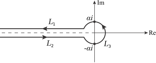
Figure 1: The contours $L_{1},L_{2},L_{3}$ which together form the Hankel contour $H_{\alpha}$

Lemma 2.1.

The meromorphic continuation of the modified Hurwitz zeta function to all $s\in\mathbb{C}$ is given by

$$\zeta_{1}(x,s)=\frac{\Gamma(1-s)}{2\pi i}\int_{H_{\alpha}}\frac{e^{xz}z^{s-1}}{e^{-z}-1}\,\mathrm{d}z,$$ (2.1)

for $\mathrm{Re}(x)>-1$, where $H_{\alpha}$ is the Hankel contour defined by Definition 2.1.

Proof.

For any $n\in\mathbb{N}$ and $s,x\in\mathbb{C}$ with $\mathrm{Re}(s)>1$ and $\mathrm{Re}(x)>-1$, we have

$$\frac{1}{(n+x)^{s}}=\frac{1}{\Gamma(s)}\int_{0}^{\infty}e^{-(n+x)z}z^{s-1}\,\mathrm{d}z.$$

Taking the sum over all $n\in\mathbb{N}$, and using the fact that $\sum_{n=1}^{\infty}e^{-nz}=\tfrac{1}{e^{z}-1}$ is a locally uniformly convergent series for $\mathrm{Re}(z)>0$, we find

$$\zeta_{1}(x,s)=\frac{1}{\Gamma(s)}\int_{0}^{\infty}e^{-xz}z^{s-1}\sum_{n=1}^{\infty}e^{-nz}\,\mathrm{d}z=\frac{1}{\Gamma(s)}\int_{0}^{\infty}\frac{e^{-xz}z^{s-1}}{e^{z}-1}\,\mathrm{d}z$$ (2.2)

for $\mathrm{Re}(s)>1$ and $\mathrm{Re}(x)>-1$. In what follows we shall show that the right-hand sides of equations (2.1) and (2.2) are identical and that the former is meromorphic for all $s,x\in\mathbb{C}$ with $\mathrm{Re}(x)>-1$; this will suffice to establish the required result.

For $\mathrm{Re}(s)>1$, we can let $\alpha\rightarrow 0$ in the Hankel-contour formula, so that the integral around the curved part $L_{3}$ of the contour can be computed using Cauchy’s theorem:

$$\int_{L_{3}}\frac{e^{xz}z^{s-1}}{e^{-z}-1}\,\mathrm{d}z=\lim_{\alpha\rightarrow 0}\Bigg{(}\int_{-\pi/2}^{\pi/2}\frac{e^{xz}z^{s}}{e^{-z}-1}\bigg{|}_{z=\alpha e^{i\theta}}\,\mathrm{d}\theta\Bigg{)}=\lim_{\alpha\rightarrow 0}\pi\Big{(}\frac{z^{s}}{-z}\Big{)}\bigg{|}_{z=\alpha e^{i\theta}}=0.$$

Hence, the Hankel contour integral expression yields:

$$\frac{\Gamma(1-s)}{2\pi i}\int_{H_{\alpha}}\frac{e^{xz}z^{s-1}}{e^{-z}-1}\,\mathrm{d}z =\frac{\Gamma(1-s)}{2\pi i}\bigg{(}\int_{0}^{\infty}\frac{e^{-xu}u^{s-1}e^{i\pi s}}{e^{u}-1}\,\mathrm{d}u-\int_{0}^{\infty}\frac{e^{-xu}u^{s-1}e^{-i\pi s}}{e^{u}-1}\,\mathrm{d}u\bigg{)}$$

$$=\frac{\Gamma(1-s)\sin(\pi s)}{\pi}\int_{0}^{\infty}\frac{e^{-xu}u^{s-1}}{e^{u}-1}\,\mathrm{d}u$$

$$=\frac{1}{\Gamma(s)}\int_{0}^{\infty}\frac{e^{-xz}z^{s-1}}{e^{z}-1}\,\mathrm{d}z,$$

where we have used the substitutions $z=e^{i\pi}u$ along $L_{1}$ and $z=e^{-i\pi}u$ along $L_{2}$, and have replaced the dummy variable $u$ by $z$ in the final line.

Thus, we have proved that (2.1) holds as an identity for $\mathrm{Re}(s)>1$ and $\mathrm{Re}(x)>-1$. Also, the right-hand side of (2.1) is analytic for $\mathrm{Re}(x)>-1$ and all $s\in\mathbb{C}\backslash\mathbb{N}$, since the integrand is finite along the contour and entire in $x$ and $s$. ∎

Lemma 2.2.

If $s=\sigma+it$ is a complex variable with $\sigma,t\in\mathbb{R}$ and $\sigma>0$, and $x$ is a real variable with $0<x<\infty$, then the modified Hurwitz zeta function $\zeta_{1}(x,s)$ can be expressed as

$$\zeta_{1}(x,s)=\frac{\chi(s)}{(2\pi)^{s}}\Bigg{(}\int_{0}^{\alpha}\frac{e^{i(1+x)u}-e^{-ixu}}{1-e^{iu}}u^{s-1}\,\mathrm{d}u\\ +e^{i\pi s/2}\int_{-i\alpha}^{\infty e^{i\phi_{2}}}\frac{e^{-(1+x)z}}{1-e^{-z}}z^{s-1}\,\mathrm{d}z+e^{-i\pi s/2}\int_{i\alpha}^{\infty e^{i\phi_{1}}}\frac{e^{-(1+x)z}}{1-e^{-z}}z^{s-1}\,\mathrm{d}z\Bigg{)},$$ (2.3)

for any given $\alpha,\phi_{1},\phi_{2}$ with $0<\alpha<2\pi$ and $-\tfrac{\pi}{2}<\phi_{1},\phi_{2}<\tfrac{\pi}{2}$.

Proof.

We start with the expression (2.1) for $\zeta_{1}(x,s)$, and split the Hankel contour into the three parts $L_{1}$, $L_{2}$, $L_{3}$ defined in Definition 2.1.

Firstly, by using Cauchy’s theorem and then substituting $z=e^{i\pi}u,z=e^{-i\pi}u$ respectively, the integrals along $L_{1}$ and $L_{2}$ become:

$$\int_{L_{1}}\frac{e^{xz}z^{s-1}}{e^{-z}-1}\,\mathrm{d}z =\int_{i\alpha}^{\infty e^{i\pi}}\frac{e^{(1+x)z}z^{s-1}}{1-e^{z}}\,\mathrm{d}z=e^{i\pi s}\int_{-i\alpha}^{\infty}\frac{e^{-(1+x)u}}{1-e^{-u}}u^{s-1}\,\mathrm{d}u;$$

$$\int_{L_{2}}\frac{e^{xz}z^{s-1}}{e^{-z}-1}\,\mathrm{d}z =-\int_{-i\alpha}^{\infty e^{-i\pi}}\frac{e^{(1+x)z}z^{s-1}}{1-e^{z}}\,\mathrm{d}z=-e^{-i\pi s}\int_{i\alpha}^{\infty}\frac{e^{-(1+x)u}}{1-e^{-u}}u^{s-1}\,\mathrm{d}u.$$

For the integral along $L_{3}$, we split the integrand as follows:

$$\int_{L_{3}}\frac{e^{xz}z^{s-1}}{e^{-z}-1}\,\mathrm{d}z=-\int_{L_{3}}\frac{e^{-(1+x)z}}{1-e^{-z}}z^{s-1}\,\mathrm{d}z+\int_{L_{3}}\frac{e^{-(1+x)z}-e^{xz}}{1-e^{-z}}z^{s-1}\,\mathrm{d}z.$$

By Cauchy’s theorem, the first of these integrals can be written as $\int_{L_{3}}=\int_{-i\alpha}^{\infty}-\int_{i\alpha}^{\infty}$. The integrand of the second integral behaves like $-(1+2x)z^{s-1}$ for $z$ close to $0$, so the integral of this function is finite even around $z=0$ (since we have assumed $\mathrm{Re}(s)>0$). This means the contour of integration can be deformed to the straight line-segment from $-i\alpha$ to $i\alpha$, and the integral can be simplified as follows:

$$\int_{-i\alpha}^{0}\frac{e^{-(1+x)z}-e^{xz}}{1-e^{-z}}z^{s-1}\,\mathrm{d}z+\int_{0}^{i\alpha}\frac{e^{-(1+x)z}-e^{xz}}{1-e^{-z}}z^{s-1}\,\mathrm{d}z$$

$$= -e^{-i\pi s/2}\int_{0}^{\alpha}\frac{e^{i(1+x)u}-e^{-ixu}}{1-e^{iu}}u^{s-1}\,\mathrm{d}u+e^{i\pi s/2}\int_{0}^{\alpha}\frac{e^{-i(1+x)u}-e^{ixu}}{1-e^{-iu}}u^{s-1}\,\mathrm{d}u$$

$$= -e^{-i\pi s/2}\int_{0}^{\alpha}\frac{e^{i(1+x)u}-e^{-ixu}}{1-e^{iu}}u^{s-1}\,\mathrm{d}u+e^{i\pi s/2}\int_{0}^{\alpha}\frac{e^{-ixu}-e^{i(1+x)u}}{e^{iu}-1}u^{s-1}\,\mathrm{d}u$$

$$= 2i\sin(\tfrac{\pi s}{2})\int_{0}^{\alpha}\frac{e^{i(1+x)u}-e^{-ixu}}{1-e^{iu}}u^{s-1}\,\mathrm{d}u.$$

Summing up the expressions derived for the integrals along $L_{1}$, $L_{2}$, and $L_{3}$, we find that (2.1) yields:

$$\begin{split}\zeta_{1}(x,s)&=\frac{\Gamma(1-s)}{2\pi i}\bigg{(}e^{i\pi s}\int_{-i\alpha}^{\infty}\frac{e^{-(1+x)u}}{1-e^{-u}}u^{s-1}\,\mathrm{d}u-e^{-i\pi s}\int_{i\alpha}^{\infty}\frac{e^{-(1+x)u}}{1-e^{-u}}u^{s-1}\,\mathrm{d}u\\ &\hskip 85.35826pt+\int_{i\alpha}^{\infty}\frac{e^{-(1+x)z}}{1-e^{-z}}z^{s-1}\,\mathrm{d}z-\int_{-i\alpha}^{\infty}\frac{e^{-(1+x)z}}{1-e^{-z}}z^{s-1}\,\mathrm{d}z\\ &\hskip 142.26378pt+2i\sin(\tfrac{\pi s}{2})\int_{0}^{\alpha}\frac{e^{i(1+x)u}-e^{-ixu}}{1-e^{iu}}u^{s-1}\,\mathrm{d}u\bigg{)}\end{split}$$

$$\begin{split}&=\tfrac{\Gamma(1-s)}{\pi}\sin(\tfrac{\pi s}{2})\bigg{(}e^{i\pi s/2}\int_{-i\alpha}^{\infty}\frac{e^{-(1+x)z}}{1-e^{-z}}z^{s-1}\,\mathrm{d}z+e^{-i\pi s/2}\int_{i\alpha}^{\infty}\frac{e^{-(1+x)z}}{1-e^{-z}}z^{s-1}\,\mathrm{d}z\\ &\hskip 227.62204pt+\int_{0}^{\alpha}\frac{e^{i(1+x)u}-e^{-ixu}}{1-e^{iu}}u^{s-1}\,\mathrm{d}u\bigg{)}.\end{split}$$

In the final expression above, the integrands of the first two integrals decay exponentially as $z$ tends to infinity in the right half plane. Thus, by Cauchy’s theorem, the upper limits of these integrals can be replaced by $\infty e^{i\phi_{1}}$ and $\infty e^{i\phi_{2}}$ respectively for any $\phi_{1},\phi_{2}\in\big{(}\tfrac{-\pi}{2},\tfrac{\pi}{2}\big{)}$. The expression outside the large parentheses is precisely $\tfrac{\chi(s)}{(2\pi)^{s}}$, so the result follows. ∎

Definition 2.2.

For $a,b\in\mathbb{R}$ with $a<b$, the curves $C_{a}^{b}$ and $\hat{C}_{b}^{a}$ are defined as follows:

$$C_{a}^{b} =\bigg{\{}\frac{i(a+b)}{2}+\frac{b-a}{2}e^{i\theta}\,:\,\theta\in\Big{(}-\frac{\pi}{2},\frac{\pi}{2}\Big{)}\bigg{\}};$$

$$\hat{C}_{b}^{a} =\bigg{\{}\frac{i(a+b)}{2}+\frac{b-a}{2}e^{i\theta}\,:\,\theta\in\Big{(}-\pi,-\frac{\pi}{2}\Big{)}\cup\Big{(}\frac{\pi}{2},\pi\Big{)}\bigg{\}}.$$

In other words, $C_{a}^{b}$ is the semicircular contour from $ia$ to $ib$ passing upwards through the right half plane, while $\hat{C}_{b}^{a}$ is the semicircular contour from $ib$ to $ia$ passing downwards through the left half plane. The two together form a full circular contour, as shown in Figure 2.

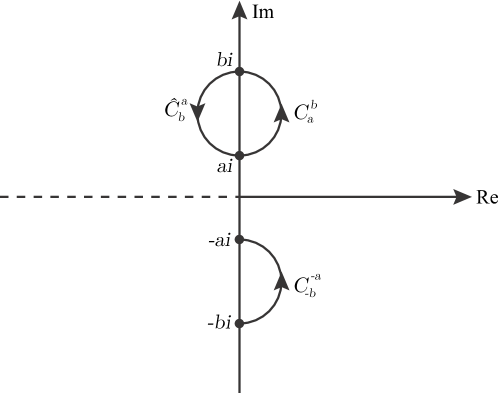
Figure 2: The contours $C_{a}^{b}$, $\hat{C}_{b}^{a}$, and $C_{-b}^{-a}$

Theorem 2.1.

If $s=\sigma+it$ is a complex variable with $\sigma,t\in\mathbb{R},0<\sigma\leq 1,0<t<\infty$, and $x$ is a real variable with $0<x<\infty$, then the modified Hurwitz zeta function $\zeta_{1}(x,s)$ can be expressed as

$$\zeta_{1}(x,s)=\chi(s)\Bigg{(}\sum_{m=1}^{\lfloor\eta/2\pi\rfloor}e^{-2\pi imx}m^{s-1}-G_{B}(\sigma,t;\eta;x)+G_{L}(\sigma,t;\eta;x)+G_{U}(\sigma,t;\eta;x)\Bigg{)},$$ (2.4)

for any given $\eta,\phi_{1},\phi_{2}$ with $0<\eta<\infty$ and $-\frac{\pi}{2}<\phi_{1},\phi_{2}<\frac{\pi}{2}$, where

$$G_{B}(\sigma,t;\eta;x) \coloneqq\tfrac{e^{-i\pi s/2}}{(2\pi)^{s}}\int_{\hat{C}^{0}_{\eta}}\frac{e^{(1+x)z}-e^{-xz}}{1-e^{z}}z^{s-1}\,\mathrm{d}z,$$ (2.5)

$$G_{L}(\sigma,t;\eta;x) \coloneqq\tfrac{e^{i\pi s/2}}{(2\pi)^{s}}\int_{-i\eta}^{\infty e^{i\phi_{2}}}\frac{e^{-(1+x)z}}{1-e^{-z}}z^{s-1}\,\mathrm{d}z,$$ (2.6)

$$G_{U}(\sigma,t;\eta;x) \coloneqq\tfrac{e^{-i\pi s/2}}{(2\pi)^{s}}\int_{i\eta}^{\infty e^{i\phi_{1}}}\frac{e^{-(1+x)z}}{1-e^{-z}}z^{s-1}\,\mathrm{d}z.$$ (2.7)

Proof.

We start with the result of Lemma 2.2. By Cauchy’s theorem, the contours of integrations in the second and third integrals in (2.3) can be deformed so as to run first from $\pm i\alpha$ to $\pm i\eta$ and then out to infinity:

$$\int_{-i\alpha}^{\infty e^{i\phi_{2}}}=-\int_{C_{-\eta}^{-\alpha}}+\int_{-i\eta}^{\infty e^{i\phi_{2}}}\,\text{ and }\,\int_{i\alpha}^{\infty e^{i\phi_{1}}}=\int_{C_{\alpha}^{\eta}}+\int_{i\eta}^{\infty e^{i\phi_{1}}}.$$

Hence, the sum of the last two terms in (2.3) is equal to the sum of $(2\pi)^{s}G_{L}(\sigma,t;\eta;x)$ and $(2\pi)^{s}G_{U}(\sigma,t;\eta;x)$ with the following expression:

$$-e^{i\pi s/2}\int_{C_{-\eta}^{-\alpha}}\frac{e^{-(1+x)z}}{1-e^{-z}}z^{s-1}\,\mathrm{d}z+e^{-i\pi s/2}\int_{C_{\alpha}^{\eta}}\frac{e^{-(1+x)z}}{1-e^{-z}}z^{s-1}\,\mathrm{d}z.$$ (2.8)

The first term of this expression, after the substitution $z=ue^{-i\pi}$, becomes

$$-e^{-i\pi s/2}\int_{\hat{C}_{\eta}^{\alpha}}\frac{e^{(1+x)u}}{1-e^{u}}u^{s-1}\,\mathrm{d}u$$

$$=\, e^{-i\pi s/2}\int_{\hat{C}_{\eta}^{\alpha}}\frac{e^{xu}}{1-e^{-u}}u^{s-1}\,\mathrm{d}u$$

$$=\, e^{-i\pi s/2}\int_{\hat{C}_{\eta}^{\alpha}}\frac{e^{-(1+x)z}}{1-e^{-z}}z^{s-1}\,\mathrm{d}z+e^{-i\pi s/2}\int_{\hat{C}_{\eta}^{\alpha}}\frac{e^{xz}-e^{-(1+x)z}}{1-e^{-z}}z^{s-1}\,\mathrm{d}z.$$

So the expression (2.8) can be rewritten as:

$$e^{-i\pi s/2}\int_{C^{\prime}}\frac{e^{-(1+x)z}}{1-e^{-z}}z^{s-1}\,\mathrm{d}z+e^{-i\pi s/2}\int_{\hat{C}_{\eta}^{\alpha}}\frac{e^{xz}-e^{-(1+x)z}}{1-e^{-z}}z^{s-1}\,\mathrm{d}z,$$

where $C^{\prime}$ is the circle with centre $\tfrac{\alpha+\eta}{2}$ formed by combining the two semicircles $C_{\alpha}^{\eta}$ and $\hat{C}_{\eta}^{\alpha}$. By the residue theorem, we can compute this circular integral explicitly:

$$\int_{C^{\prime}}\frac{e^{-(1+x)z}}{1-e^{-z}}z^{s-1}\,\mathrm{d}z=\sum_{m=1}^{\lfloor\eta/2\pi\rfloor}2\pi i\mathrm{Res}_{2\pi mi}\bigg{(}\frac{e^{-(1+x)z}}{1-e^{-z}}z^{s-1}\bigg{)}=\sum_{m=1}^{\lfloor\eta/2\pi\rfloor}e^{-2\pi imx}m^{s-1}(2\pi i)^{s}.$$

So the expression (2.8) can be rewritten as:

$$(2\pi)^{s}\sum_{m=1}^{\lfloor\eta/2\pi\rfloor}e^{-2\pi imx}m^{s-1}+e^{-i\pi s/2}\int_{\hat{C}_{\eta}^{\alpha}}\frac{e^{xz}-e^{-(1+x)z}}{1-e^{-z}}z^{s-1}\,\mathrm{d}z$$

$$=\, (2\pi)^{s}\sum_{m=1}^{\lfloor\eta/2\pi\rfloor}e^{-2\pi imx}m^{s-1}+e^{-i\pi s/2}\int_{\hat{C}_{\eta}^{0}}\frac{e^{xz}-e^{-(1+x)z}}{1-e^{-z}}z^{s-1}\,\mathrm{d}z+e^{-i\pi s/2}\int_{0}^{i\alpha}\frac{e^{xz}-e^{-(1+x)z}}{1-e^{-z}}z^{s-1}\,\mathrm{d}z.$$

The last term of this expression, after substituting $z=iu$, becomes exactly minus the first integral in (2.3). Hence, starting from the formula (2.3) for $\zeta_{1}(x,s)$, we find:

$$\zeta_{1}(x,s) =\frac{\chi(s)}{(2\pi)^{s}}\bigg{(}\int_{0}^{\alpha}\frac{e^{i(1+x)u}-e^{-ixu}}{1-e^{iu}}u^{s-1}\,\mathrm{d}u+(2\pi)^{s}G_{L}(\sigma,t;\eta;x)+(2\pi)^{s}G_{U}(\sigma,t;\eta;x)+(\ref{C-curve-integrals})\bigg{)}$$

$$\begin{split}&=\frac{\chi(s)}{(2\pi)^{s}}\bigg{(}(2\pi)^{s}G_{L}(\sigma,t;\eta;x)+(2\pi)^{s}G_{U}(\sigma,t;\eta;x)+(2\pi)^{s}\sum_{m=1}^{\lfloor\eta/2\pi\rfloor}e^{-2\pi imx}m^{s-1}\\ &\hskip 199.16928pt+e^{-i\pi s/2}\int_{\hat{C}_{\eta}^{0}}\frac{e^{xz}-e^{-(1+x)z}}{1-e^{-z}}z^{s-1}\,\mathrm{d}z\bigg{)}\end{split}$$

$$=\chi(s)\bigg{(}\sum_{m=1}^{\lfloor\eta/2\pi\rfloor}e^{-2\pi imx}m^{s-1}+G_{L}(\sigma,t;\eta;x)+G_{U}(\sigma,t;\eta;x)-G_{B}(\sigma,t;\eta;x)\bigg{)},$$

as required. ∎

Remark 2.1.

For the particular case of $x=0$, we find

$$G_{B}(\sigma,t;\eta;0)=\tfrac{e^{-i\pi s/2}}{(2\pi)^{s}}\int_{\hat{C}^{0}_{\eta}}\big{(}-z^{s-1}\big{)}\,\mathrm{d}z=\frac{1}{(2\pi)^{s}}\Big{(}-\frac{\eta^{s}}{s}\Big{)},$$

and therefore the identity (2.4) reduces, as expected, to the formula (1.4) proved in [4].

In the remainder of this paper, we shall construct the large-$t$ asymptotics of each of $G_{L},G_{U},G_{B}$, and hence derive a large-$t$ asymptotic formula for $\zeta_{1}(x,s)$.

Lemma 2.3.

The function $D_{N}$ defined by

$$D_{N}(z;\xi;\sigma,t)\coloneqq\big{(}\tfrac{\mathrm{d}}{\mathrm{d}z}\cdot\tfrac{1}{\xi-\frac{it}{z}}\big{)}^{N}(z^{\sigma-1})$$ (2.9)

can be expressed in the following form for any $N\geq 0$:

$$D_{N}=\sum_{b=0}^{N}\sum_{c=0}^{N}A_{bc}^{(N)}\Bigg{(}\frac{t^{b}\xi^{N-b}\sigma^{c}z^{N-b}}{(\xi z-it)^{2N}}\Bigg{)}z^{\sigma-1},$$ (2.10)

where $A_{bc}^{(N)}$ is a Gaussian integer with absolute value $\leq(2N-1)!!\coloneqq(1)(3)(5)\dots(2N-3)(2N-1)$ for each $b,c$.

Proof.

Following the argument of [4], we proceed by induction on $N$.

In the base case $N=0$, we must also have $b=c=0$ and so the expression (2.10) reduces to

$$D_{N}=A_{00}^{(0)}\Bigg{(}\frac{t^{0}\xi^{0}\sigma^{0}z^{0}}{(\xi z-it)^{0}}\Bigg{)}z^{\sigma-1}=A_{00}^{(0)}z^{\sigma-1}.$$

By (2.9), this is valid with $A_{00}^{(0)}=1=(-1)!!$. (It makes sense to define $(-1)!!=1$ in the same way as we ordinarily define $0!=1$, because $(2N+1)!!=(2N-1)!!(2N+1)$ for all $N$ and $1!!=1$.)

Now assume that $D_{N}$ can be written in the form (2.10) for some fixed $N\geq 0$, and consider $D_{N+1}$. Using the definition (2.9), we have:

$$D_{N+1} =\frac{\mathrm{d}}{\mathrm{d}z}\bigg{(}\frac{D_{N}}{\xi-\tfrac{it}{z}}\bigg{)}=\frac{\mathrm{d}}{\mathrm{d}z}\bigg{(}\frac{zD_{N}}{\xi z-it}\bigg{)}$$

$$=\frac{\mathrm{d}}{\mathrm{d}z}\Bigg{(}\sum_{b=0}^{N}\sum_{c=0}^{N}A_{bc}^{(N)}\Bigg{(}\frac{t^{b}\xi^{N-b}\sigma^{c}z^{N+1-b}}{(\xi z-it)^{2N+1}}\Bigg{)}z^{\sigma-1}\Bigg{)}$$

$$=\sum_{b=0}^{N}\sum_{c=0}^{N}A_{bc}^{(N)}\frac{\big{[}t^{b}\xi^{N-b}\sigma^{c}(N+\sigma-b)z^{N+\sigma-b-1}\big{]}(\xi z-it)-\big{[}t^{b}\xi^{N-b}\sigma^{c}z^{N+\sigma-b}\big{]}(2N+1)\xi}{(\xi z-it)^{2N+2}}$$

$$=\sum_{b=0}^{N}\sum_{c=0}^{N}A_{bc}^{(N)}\frac{t^{b}\xi^{N+1-b}\sigma^{c}(-N-1+\sigma-b)z^{N+\sigma-b}-it^{b+1}\xi^{N-b}\sigma^{c}(N+\sigma-b)z^{N+\sigma-b-1}}{(\xi z-it)^{2N+2}}$$

$$\begin{split}&=\sum_{b=0}^{N}\sum_{c=0}^{N}\Bigg{(}-(N+1+b)A_{bc}^{(N)}\frac{t^{b}\xi^{N+1-b}\sigma^{c}z^{N+1-b}}{(\xi z-it)^{2N+2}}+A_{bc}^{(N)}\frac{t^{b}\xi^{N+1-b}\sigma^{c+1}z^{N+1-b}}{(\xi z-it)^{2N+2}}\\ &\hskip 85.35826pt-i(N-b)A_{bc}^{(N)}\frac{t^{b+1}\xi^{N-b}\sigma^{c}z^{N-b}}{(\xi z-it)^{2N+2}}-iA_{bc}^{(N)}\frac{t^{b+1}\xi^{N-b}\sigma^{c+1}z^{N-b}}{(\xi z-it)^{2N+2}}\Bigg{)}z^{\sigma-1}.\end{split}$$

Thus, setting the values of $A_{bc}^{(N+1)}$ as suggested by this expression, we obtain a formula for $D_{N+1}$ in the form of (2.10). ∎

Assumption 2.1.

We shall fix $\epsilon>0$ and assume that the variable $\eta$ is never, for any integer $n$, within a factor of $1\pm\epsilon$ of the quantity $\tfrac{t}{x+n}$. In other words, we assume that

$$\forall n\in\mathbb{Z},\;\text{ either }\;\eta>(1+\epsilon)\tfrac{t}{x+n}\;\text{ or }\;\eta<(1-\epsilon)\tfrac{t}{x+n}.$$

The above assumption can be rewritten as

$$\mathrm{dist}\Big{(}x-\frac{t}{\eta},\mathbb{Z}\Big{)}>\frac{\epsilon t}{\eta},$$

or equivalently as

$$\forall n\in\mathbb{Z},\;\big{|}(x+n)\eta-t\big{|}>\epsilon t.$$ (2.11)

Note that to find out whether a given $\eta$ satisfies (2.11), it suffices to check for the particular value of $n$ such that $|(x+n)\eta-t|$ is minimal, i.e. for $n=\lfloor\tfrac{t}{\eta}-x+\tfrac{1}{2}\rfloor$, the closest integer to $\tfrac{t}{\eta}-x$. This $n$ may be either a positive or negative integer, depending on the values of $x$, $t$, and $\eta$.

3 Asymptotics for $G_{L}$

The series $\sum_{n=0}^{\infty}e^{-nz}=\frac{1}{1-e^{-z}}$ is locally uniformly convergent for $\mathrm{Re}(z)>0$, so we can interchange the series and integral to obtain

$$G_{L}(\sigma,t;\eta;x)=\tfrac{e^{i\pi s/2}}{(2\pi)^{s}}\sum_{n=1}^{\infty}\int_{-i\eta}^{\infty e^{i\phi_{2}}}e^{-(x+n)z}z^{s-1}\,\mathrm{d}z.$$ (3.1)

Repeatedly integrating by parts in the summand gives

$$\int_{-i\eta}^{\infty e^{i\phi_{2}}}e^{-(x+n)z}z^{s-1}\,\mathrm{d}z=\sum_{j=0}^{N-1}e^{-(x+n)z+it\log z}\Big{(}\tfrac{1}{x+n-\frac{it}{z}}\cdot\tfrac{\mathrm{d}}{\mathrm{d}z}\Big{)}^{j}\Big{(}\tfrac{z^{\sigma-1}}{x+n-\frac{it}{z}}\Big{)}\Bigg{|}_{z=-i\eta}\\ +\int_{-i\eta}^{\infty e^{i\phi_{2}}}e^{-(x+n)z+it\log z}D_{N}(z;x+n;\sigma,t)\,\mathrm{d}z$$ (3.2)

for any $N\in\mathbb{N}$, where $D_{N}$ is defined by (2.9).

In what follows, we shall take $\phi_{2}=0$, so that $z\in-i\eta+\mathbb{R}^{+}$.

Lemma 3.1.

$D_{N}$ can be uniformly estimated in either of the following ways, both valid for $\mathrm{Im}(z)<0$ and $\xi>0$:

$$D_{N}(z;\xi;\sigma,t) =O\big{(}(2N-1)!!(N+1)^{2}|z|^{\sigma-N-1}\xi^{-N}\big{)};$$ (3.3)

$$D_{N}(z;\xi;\sigma,t) =O\big{(}(2N-1)!!(N+1)^{2}|z|^{\sigma-1}t^{-N}\big{)}.$$ (3.4)

Proof.

By (2.10), we have the following two expressions for $D_{N}$:

$$D_{N}(z;\xi;\sigma,t) =O\Bigg{(}(2N-1)!!|z|^{\sigma-1}\sum_{b=0}^{N}\sum_{c=0}^{N}\Big{|}\tfrac{t}{\xi z}\Big{|}^{b}|\sigma|^{c}\Big{|}\tfrac{\xi z}{(\xi z-it)^{2}}\Big{|}^{N}\Bigg{)};$$

$$D_{N}(z;\xi;\sigma,t) =O\Bigg{(}(2N-1)!!|z|^{\sigma-1}\sum_{b=0}^{N}\sum_{c=0}^{N}\Big{|}\tfrac{\xi z}{t}\Big{|}^{N-b}|\sigma|^{c}\Big{|}\tfrac{t}{(\xi z-it)^{2}}\Big{|}^{N}\Bigg{)}.$$

Since $0<\sigma\leq 1$ and $|\xi z-it|$ is greater than both $|\xi z|$ and $t$ (by our assumption on $z$ and the fact that $\xi$ and $t$ are positive reals), we can simplify these estimates as follows.

Case 1: $\boldsymbol{|\xi z|>t}.$

In this case,

$$D_{N} =O\Bigg{(}(2N-1)!!|z|^{\sigma-1}\sum_{b=0}^{N}\Big{|}\tfrac{t}{\xi z}\Big{|}^{b}(N+1)\Big{|}\tfrac{\xi z}{(\xi z)^{2}}\Big{|}^{N}\Bigg{)}=O\Big{(}(2N-1)!!(N+1)^{2}|z|^{\sigma-N-1}\xi^{-N}\Big{)}.$$

Case 2: $\boldsymbol{|\xi z|<t}.$

In this case,

$$D_{N} =O\Bigg{(}(2N-1)!!|z|^{\sigma-1}\sum_{b=0}^{N}\Big{|}\tfrac{\xi z}{t}\Big{|}^{N-b}(N+1)\big{|}\tfrac{t}{t^{2}}\big{|}^{N}\Bigg{)}=O\Big{(}(2N-1)!!(N+1)^{2}|z|^{\sigma-1}t^{-N}\Big{)}.$$

In both cases, we have $D_{N}=O\Big{(}(2N-1)!!(N+1)^{2}|z|^{\sigma-1}\max\big{(}\xi|z|,t\big{)}^{-N}\Big{)}$, from which both the estimates (3.3), (3.4) follow. Note also that in each case the bound is uniform in all variables: in fact, the $O$-constant can be taken to be $1$. ∎

Lemma 3.2.

We have the following estimate for $G_{L}$, uniform in $\sigma$, $t$, $\eta$, $x$, and $N\geq 1$:

$$G_{L}(\sigma,t;\eta;x)=\frac{e^{i\pi\sigma/2}e^{it\log\eta}}{(2\pi)^{s}}\sum_{n=1}^{M}\sum_{j=0}^{N-1}e^{i(x+n)\eta}\Bigg{[}\Big{(}\tfrac{1}{x+n-\frac{it}{z}}\cdot\tfrac{\mathrm{d}}{\mathrm{d}z}\Big{)}^{j}\Big{(}\tfrac{z^{\sigma-1}}{x+n-\frac{it}{z}}\Big{)}\Bigg{]}_{z=-i\eta}\\ +O\Big{(}(2N-1)!!(N+1)^{2}\eta^{\sigma-N-1}\Big{)},$$

where $M$ is a finite number depending only on $N$ and $\eta$.

Proof.

Employing (3.1) and (3.2) (where we have set $\phi_{2}=0$), it suffices to estimate

$$\sum_{n=1}^{\infty}\int_{-i\eta}^{\infty}e^{-(x+n)z+it\log z}D_{N}(z;x+n;\sigma,t)\,\mathrm{d}z,$$

which can be achieved using Lemma 3.1. By equation (3.3), this expression is given by:

$$O \Bigg{(}\sum_{n=1}^{\infty}\int_{-i\eta}^{\infty}e^{-(x+n)z+it\log z}(2N-1)!!(N+1)^{2}|z|^{\sigma-N-1}(x+n)^{-N}\,\mathrm{d}z\Bigg{)}$$

$$=O \Bigg{(}(2N-1)!!(N+1)^{2}\sum_{n=1}^{\infty}\int_{-i\eta}^{\infty}e^{-(x+n)\mathrm{Re}(z)}e^{\pi t/2}\eta^{\sigma-N-1}(x+n)^{-N}\,\mathrm{d}z\Bigg{)}$$

$$=O \Bigg{(}(2N-1)!!(N+1)^{2}e^{\pi t/2}\eta^{\sigma-N-1}\sum_{n=1}^{\infty}(x+n)^{-N}\int_{0}^{\infty}e^{-(x+n)u}\,\mathrm{d}z\Bigg{)}$$

$$=O \Bigg{(}(2N-1)!!(N+1)^{2}e^{\pi t/2}\eta^{\sigma-N-1}\sum_{n=1}^{\infty}(x+n)^{-N-1}\Bigg{)}=O\Big{(}(2N-1)!!(N+1)^{2}e^{\pi t/2}\eta^{\sigma-N-1}\Big{)}.$$

Since $e^{i\pi s/2}=e^{i\pi\sigma/2}e^{-\pi t/2}$ and $e^{it\log(-i\eta)}=e^{it\log\eta}e^{\pi t/2}$, using the above estimate together with (3.1) and (3.2) yields:

$$G_{L}(\sigma,t;\eta;x) =\tfrac{e^{i\pi\sigma/2}e^{-\pi t/2}}{(2\pi)^{s}}\sum_{n=1}^{\infty}\int_{-i\eta}^{\infty e^{i\phi_{2}}}e^{-(x+n)z}z^{s-1}\,\mathrm{d}z$$

$$\begin{split}&=\frac{e^{i\pi\sigma/2}e^{it\log\eta}}{(2\pi)^{s}}\sum_{n=1}^{\infty}\sum_{j=0}^{N-1}e^{i(x+n)\eta}\Bigg{[}\Big{(}\tfrac{1}{x+n-\frac{it}{z}}\cdot\tfrac{\mathrm{d}}{\mathrm{d}z}\Big{)}^{j}\Big{(}\tfrac{z^{\sigma-1}}{x+n-\frac{it}{z}}\Big{)}\Bigg{]}_{z=-i\eta}\\ &\hskip 85.35826pt+\frac{e^{i\pi\sigma/2}e^{-\pi t/2}}{(2\pi)^{s}}\sum_{n=1}^{\infty}\int_{-i\eta}^{\infty e^{i\phi_{2}}}e^{-(x+n)z+it\log z}D_{N}(z;x+n;\sigma,t)\,\mathrm{d}z\end{split}$$

$$\begin{split}&=\frac{e^{i\pi\sigma/2}e^{it\log\eta}}{(2\pi)^{s}}\sum_{n=1}^{\infty}\sum_{j=0}^{N-1}e^{i(x+n)\eta}\Bigg{[}\Big{(}\tfrac{1}{x+n-\frac{it}{z}}\cdot\tfrac{\mathrm{d}}{\mathrm{d}z}\Big{)}^{j}\Big{(}\tfrac{z^{\sigma-1}}{x+n-\frac{it}{z}}\Big{)}\Bigg{]}_{z=-i\eta}\\ &\hskip 199.16928pt+O\Big{(}(2N-1)!!(N+1)^{2}\eta^{\sigma-N-1}\Big{)}.\end{split}$$

The uniformity of the $O$-bound is inherited from Lemma 3.1. In order to derive the final result, we just need to find $M(N,\eta)$ large enough so that

$$\sum_{n=M+1}^{\infty}\sum_{j=0}^{N-1}e^{i(x+n)\eta}\Bigg{[}\Big{(}\tfrac{1}{x+n-\frac{it}{z}}\cdot\tfrac{\mathrm{d}}{\mathrm{d}z}\Big{)}^{j}\Big{(}\tfrac{z^{\sigma-1}}{x+n-\frac{it}{z}}\Big{)}\Bigg{]}_{z=-i\eta}=O\Big{(}(2N-1)!!(N+1)^{2}\eta^{\sigma-N-1}\Big{)}.$$ (3.5)

Using the definition of $D_{N}$ and the bound (3.3) for $D_{N}$, we can estimate the left hand side of (3.5) as follows:

$${\color[rgb]{1,1,1}=}\sum_{n=M+1}^{\infty}\sum_{j=0}^{N-1}\frac{e^{i(x+n)\eta}}{x+n+\frac{t}{\eta}}D_{j}(-i\eta;x+n;\sigma,t)$$

$$=\sum_{n=M+1}^{\infty}\frac{e^{i(x+n)\eta}(-i\eta)^{\sigma-1}}{x+n+\frac{t}{\eta}}+\sum_{n=M+1}^{\infty}\sum_{j=1}^{N-1}O\bigg{(}\frac{1}{x+n+\frac{t}{\eta}}(2j-1)!!(j+1)^{2}\eta^{\sigma-j-1}(x+n)^{-j}\bigg{)}$$

$$=O\bigg{(}\eta^{\sigma-1}\sum_{n=M+1}^{\infty}\frac{e^{in\eta}}{x+n+\frac{t}{\eta}}\bigg{)}+\sum_{j=1}^{N-1}O\bigg{(}(2j-1)!!(j+1)^{2}\eta^{\sigma-j-1}\sum_{n=M+1}^{\infty}(x+n)^{-j-1}\bigg{)}$$

$$=O\bigg{(}\eta^{\sigma-1}\sum_{n=M+1}^{\infty}\frac{e^{in\eta}}{x+n}\bigg{)}+O\bigg{(}(2N-3)!!N^{2}\sum_{j=1}^{N-1}\eta^{\sigma-j-1}\sum_{n=M+1}^{\infty}(x+n)^{-j-1}\bigg{)}.$$

All of the infinite series in this expression are convergent, so we can simply choose $M$ large enough so that

$$\sum_{n=M+1}^{\infty}\frac{e^{in\eta}}{x+n}\leq\eta^{-N}$$

and

$$\sum_{n=M+1}^{\infty}(x+n)^{-j-1}\leq\eta^{j-N}$$

for $j=1,2,\dots,N-1$. In the second of these inequalities, the left hand side is decreasing in $j$ while the right hand side is increasing in $j$, so we can simplify the conditions to

$$\sum_{n=M+1}^{\infty}e^{in\eta}n^{-1}\leq\eta^{-N}$$ (3.6)

and

$$\sum_{n=M+1}^{\infty}n^{-2}\leq\eta^{1-N}.$$ (3.7)

For any $M$ satisfying (3.6) and (3.7), we have the required bound (3.5), and so the final result holds. ∎

4 Asymptotics for $G_{U}$

As before, the series $\sum_{n=0}^{\infty}e^{-nz}=\frac{1}{1-e^{-z}}$ is locally uniformly convergent for $\mathrm{Re}(z)>0$, so we can interchange the series and integral to obtain

$$G_{U}(\sigma,t;\eta;x)=\tfrac{e^{-i\pi s/2}}{(2\pi)^{s}}\sum_{n=1}^{\infty}\int_{i\eta}^{\infty e^{i\phi_{1}}}e^{-(x+n)z}z^{s-1}\,\mathrm{d}z.$$ (4.1)

Let us fix $\phi_{1}=\tfrac{\pi}{2}$, so that $z\in i[\eta,\infty)$. Now the integrand is $e^{-(x+n)z+it}z^{\sigma-1}$, which has a stationary point iff $-(x+n)+\tfrac{it}{z}=0$, i.e. at $z=\tfrac{it}{x+n}$. So there is a stationary point in the interval of integration iff

$$\tfrac{it}{x+n}\in i[\eta,\infty),\text{ i.e. }\eta\leq\tfrac{t}{x+n}<\infty,\text{ i.e. }n\leq\tfrac{t}{\eta}-x.$$

This is the first place we need to use Assumption 2.1. The inequality (2.11) can be rearranged in terms of $n$, since its opposite statement rearranges as follows:

$$|(x+n)\eta-t|\geq\epsilon t \Leftrightarrow(1-\epsilon)t\leq(x+n)\eta\leq(1+\epsilon)t$$

$$\Leftrightarrow(1-\epsilon)\tfrac{t}{\eta}-x\leq n\leq(1+\epsilon)\tfrac{t}{\eta}-x.$$

So we need to consider two separate cases, namely $n<(1-\epsilon)\tfrac{t}{\eta}-x$ and $n>(1+\epsilon)\tfrac{t}{\eta}-x$. In other words, the sum over $n$ appearing in (4.1) needs to be split into two separate subseries. When $n>(1+\epsilon)\tfrac{t}{\eta}-x$, there is no stationary point in the interval of integration and we can use integration by parts as before. When $n<(1-\epsilon)\tfrac{t}{\eta}-x$, we shall rewrite the integral along $i[\eta,\infty)$ as the difference of an integral along $i[0,\eta)$, which no longer contains a stationary point, and an integral along $i[0,\infty)$, which can be computed explicitly.

In analogy with equation (3.2), repeatedly integrating by parts in the summand of (4.1) gives

$$\int_{i\eta}^{i\infty}e^{-(x+n)z}z^{s-1}\,\mathrm{d}z=\sum_{j=0}^{N-1}e^{-(x+n)z+it\log z}\Big{(}\tfrac{1}{x+n-\frac{it}{z}}\cdot\tfrac{\mathrm{d}}{\mathrm{d}z}\Big{)}^{j}\Big{(}\tfrac{z^{\sigma-1}}{x+n-\frac{it}{z}}\Big{)}\Bigg{|}_{z=i\eta}\\ +\int_{i\eta}^{i\infty}e^{-(x+n)z+it\log z}D_{N}(z;x+n;\sigma,t)\,\mathrm{d}z.$$ (4.2)

Similarly,

$$\int_{0}^{i\eta}e^{-(x+n)z}z^{s-1}\,\mathrm{d}z=-\sum_{j=0}^{N-1}e^{-(x+n)z+it\log z}\Big{(}\tfrac{1}{x+n-\frac{it}{z}}\cdot\tfrac{\mathrm{d}}{\mathrm{d}z}\Big{)}^{j}\Big{(}\tfrac{z^{\sigma-1}}{x+n-\frac{it}{z}}\Big{)}\Bigg{|}_{z=i\eta}\\ +\int_{0}^{i\eta}e^{-(x+n)z+it\log z}D_{N}(z;x+n;\sigma,t)\,\mathrm{d}z,$$ (4.3)

each of (4.2) and (4.3) being valid for any $N\in\mathbb{N}$. To derive each of these identities, we have used the fact that for every $j$, the summand in the $\sum_{j}$ series tends to zero as $|\eta|$ tends to either $0$ or $\infty$ with $\eta$ on the imaginary axis. This follows by approximating each part of the summand, e.g. by a power of $z$.

Lemma 4.1.

If $n<(1-\epsilon)\tfrac{t}{\eta}-x$ and $z\in i[0,\eta]$, then

$$D_{N}(z;x+n;\sigma,t)=O\Big{(}(2N-1)!!(N+1)^{2}|z|^{\sigma-1}t^{-N}\epsilon^{-2N}\Big{)}.$$ (4.4)

If $n>(1+\epsilon)\tfrac{t}{\eta}-x$ and $z\in i[\eta,\infty)$, then

$$D_{N}(z;x+n;\sigma,t)=O\Big{(}(2N-1)!!(N+1)^{2}|z|^{\sigma-N-1}(x+n)^{-N}\epsilon^{-2N}(1+\epsilon)^{2N}\Big{)}.$$ (4.5)

Both of these estimates are uniform in all parameters.

Proof.

The argument here is similar to the argument used in Lemma 3.1, starting from the expression (2.10) for $D_{N}$.

Case 1: $\boldsymbol{n<(1-\epsilon)\tfrac{t}{\eta}-x,z\in i[0,\eta]}.$

In this case, $|(x+n)z|\leq(x+n)\eta<(1-\epsilon)t$, and thus

$$D_{N}(z;x+n;\sigma,t) =O\Bigg{(}(2N-1)!!|z|^{\sigma-1}\sum_{b=0}^{N}\sum_{c=0}^{N}\Big{|}\tfrac{(x+n)z}{t}\Big{|}^{N-b}|\sigma|^{c}\Big{|}\tfrac{t}{((x+n)z-it)^{2}}\Big{|}^{N}\Bigg{)}$$

$$=O\bigg{(}(2N-1)!!(N+1)^{2}|z|^{\sigma-1}\Big{|}\tfrac{t}{((x+n)z-it)^{2}}\Big{|}^{N}\bigg{)}.$$

Since $(x+n)z$ is positive imaginary with modulus at most $(1-\epsilon)t$, it follows that $\big{|}(x+n)z-it\big{|}>\epsilon t$, and thus

$$D_{N} =O\Big{(}(2N-1)!!(N+1)^{2}|z|^{\sigma-1}t^{N}(\epsilon t)^{-2N}\Big{)},$$

as required.

Case 2: $\boldsymbol{n>(1+\epsilon)\tfrac{t}{\eta}-x,z\in i[\eta,\infty)}.$

In this case, $|(x+n)z|\geq(x+n)\eta>(1+\epsilon)t$, and thus

$$D_{N}(z;x+n;\sigma,t) =O\Bigg{(}(2N-1)!!|z|^{\sigma-1}\sum_{b=0}^{N}\sum_{c=0}^{N}\Big{|}\tfrac{t}{(x+n)z}\Big{|}^{b}|\sigma|^{c}\Big{|}\tfrac{(x+n)z}{((x+n)z-it)^{2}}\Big{|}^{N}\Bigg{)}$$

$$=O\bigg{(}(2N-1)!!(N+1)^{2}|z|^{\sigma-1}\Big{|}\tfrac{(x+n)z}{((x+n)z-it)^{2}}\Big{|}^{N}\bigg{)}.$$

Since $(x+n)z$ is positive imaginary with modulus at least $(1+\epsilon)t$, it follows that $\big{|}(x+n)z-it\big{|}>\tfrac{\epsilon}{1+\epsilon}\big{|}(x+n)z\big{|}$, and thus

$$D_{N} =O\Big{(}(2N-1)!!(N+1)^{2}|z|^{\sigma-1}\big{|}(x+n)z\big{|}^{-N}\big{(}\tfrac{\epsilon}{1+\epsilon}\big{)}^{-2N}\Big{)},$$

which yields the desired estimate.

As in Lemma 3.1, all bounds are uniform and the $O$-constants can be taken to be $1$. ∎

Lemma 4.2.

We have the following two estimates, uniform in $\sigma$, $t$, $\eta$, $x$, $\epsilon$, and $N\geq 1$ satisfying Assumption 2.1:

$$\sum_{n=1}^{\big{\lfloor}\tfrac{t}{\eta}-x\big{\rfloor}}\int_{0}^{i\eta}e^{-(x+n)z+it\log z}D_{N}(z;x+n;\sigma,t)\,\mathrm{d}z=O\big{(}(2N+1)!!(N+1)^{2}e^{-\pi t/2}\sigma^{-1}\eta^{\sigma-N-1}\epsilon^{-2N-2}\big{)},$$

and

$$\sum_{n=\big{\lceil}\tfrac{t}{\eta}-x\big{\rceil}}^{\infty}\int_{i\eta}^{i\infty}e^{-(x+n)z+it\log z}D_{N}(z;x+n;\sigma,t)\,\mathrm{d}z=O\big{(}(2N+1)!!(N+1)^{2}e^{-\pi t/2}\eta^{\sigma-N-1}\epsilon^{-2N-2}(1+\epsilon)^{2N+2}\big{)}.$$

Proof.

We shall use the estimates from Lemma 4.1. Let ${}_{U}I_{1}$ and ${}_{U}I_{2}$ denote the two expressions we need to estimate. First, by (4.4) we find the following estimate:

$${}_{U}I_{1} =O\Bigg{(}\sum_{n=1}^{\big{\lfloor}\tfrac{t}{\eta}-x\big{\rfloor}}\int_{0}^{i\eta}e^{-(x+n)z+it\log z}(2N-1)!!(N+1)^{2}|z|^{\sigma-1}t^{-N}\epsilon^{-2N}\,\mathrm{d}z\Bigg{)}$$

$$=O\Bigg{(}(2N-1)!!(N+1)^{2}t^{-N}\epsilon^{-2N}\sum_{n=1}^{\big{\lfloor}\tfrac{t}{\eta}-x\big{\rfloor}}\int_{0}^{i\eta}e^{-\pi t/2}|z|^{\sigma-1}\,\mathrm{d}z\Bigg{)}$$

$$=O\Bigg{(}(2N-1)!!(N+1)^{2}e^{-\pi t/2}\big{(}\tfrac{\eta^{\sigma}}{\sigma}\big{)}t^{-N}\epsilon^{-2N}\sum_{n=1}^{\big{\lfloor}\tfrac{t}{\eta}-x\big{\rfloor}}1\Bigg{)}$$

$$=O\big{(}(2N-1)!!(N+1)^{2}e^{-\pi t/2}\sigma^{-1}\eta^{\sigma-1}t^{-N+1}\epsilon^{-2N}\big{)}.$$

We can assume $\eta<t$ (otherwise this expression is non-existent), so $t^{-N+1}<\eta^{-N+1}$ and therefore

$$_{U}I_{1}=O\big{(}(2N-1)!!(N+1)^{2}e^{-\pi t/2}\sigma^{-1}\eta^{\sigma-N}\epsilon^{-2N}\big{)}.$$ (4.6)

Applying integration by parts once to the original expression for ${}_{U}I_{1}$ gives the expression

$${}_{U}I_{1}=\sum_{n=1}^{\big{\lfloor}\tfrac{t}{\eta}-x\big{\rfloor}}\Bigg{(}-\Big{[}e^{-(x+n)z+it\log z}\Big{(}\tfrac{1}{x+n-\tfrac{it}{z}}\Big{)}D_{N}(z;x+n;\sigma,t)\Big{]}_{0}^{i\eta}\\ +\int_{0}^{i\eta}e^{-(x+n)z+it\log z}D_{N+1}(z;x+n;\sigma,t)\,\mathrm{d}z\Bigg{)}.$$

Using equation (4.4) again for the first half of this and equation (4.6) (with $N$ replaced by $N+1$) for the second half, we find:

$$\begin{split}{}_{U}I_{1}&=O\Bigg{(}\sum_{n=1}^{\big{\lfloor}\tfrac{t}{\eta}-x\big{\rfloor}}\Big{[}\tfrac{e^{-\pi t/2}z}{(x+n)z-it}(2N-1)!!(N+1)^{2}|z|^{\sigma-1}t^{-N}\epsilon^{-2N}\Big{]}_{z=i\eta}\Bigg{)}\\ &\hskip 199.16928pt+O\big{(}(2N+1)!!(N+2)^{2}e^{-\pi t/2}\sigma^{-1}\eta^{\sigma-N-1}\epsilon^{-2N-2}\big{)}\end{split}$$

$$=O\Big{(}\tfrac{e^{-\pi t/2}\eta}{\epsilon t}(2N+1)!!(N+1)\eta^{\sigma-2}t^{-N+1}\epsilon^{-2N}\Big{)}+O\big{(}(2N+1)!!(N+1)^{2}e^{-\pi t/2}\sigma^{-1}\eta^{\sigma-N-1}\epsilon^{-2N-2}\big{)}$$

$$=O\Big{(}(2N+1)!!e^{-\pi t/2}\big{[}(N+1)\eta^{\sigma-1}t^{-N}\epsilon^{-2N-1}+(N+1)^{2}\sigma^{-1}\eta^{\sigma-N-1}\epsilon^{-2N-2}\big{]}\Big{)}$$

$$=O\big{(}(2N+1)!!(N+1)^{2}e^{-\pi t/2}\sigma^{-1}\eta^{\sigma-N-1}\epsilon^{-2N-2}\big{)},$$

where we have again used the estimates $(x+n)\eta-t>\epsilon t$ and $t^{-N}<\eta^{-N}$. Once again, all $O$-constants are uniform.

Second, by (4.5) we have:

$${}_{U}I_{2} =O\Bigg{(}\sum_{n=\big{\lceil}\tfrac{t}{\eta}-x\big{\rceil}}^{\infty}\int_{i\eta}^{i\infty}e^{-(x+n)z+it\log z}(2N-1)!!(N+1)^{2}|z|^{\sigma-N-1}(x+n)^{-N}\epsilon^{-2N}(1+\epsilon)^{2N}\,\mathrm{d}z\Bigg{)}$$

$$=O\Bigg{(}(2N-1)!!(N+1)^{2}\epsilon^{-2N}(1+\epsilon)^{2N}\sum_{n=\big{\lceil}\tfrac{t}{\eta}-x\big{\rceil}}^{\infty}\int_{i\eta}^{i\infty}e^{-\pi t/2}|z|^{\sigma-N-1}(x+n)^{-N}\,\mathrm{d}z\Bigg{)}$$

$$=O\Bigg{(}(2N-1)!!(N+1)^{2}e^{-\pi t/2}(N-\sigma)^{-1}\eta^{\sigma-N}\epsilon^{-2N}(1+\epsilon)^{2N}\sum_{n=\big{\lceil}\tfrac{t}{\eta}-x\big{\rceil}}^{\infty}(x+n)^{-N}\Bigg{)}$$

$$=O\big{(}(2N-1)!!(N+1)^{2}e^{-\pi t/2}\eta^{\sigma-N}\epsilon^{-2N}(1+\epsilon)^{2N}\big{)},$$ (4.7)

provided that $N\geq 2$.

Applying integration by parts once to the original expression for ${}_{U}I_{2}$ gives the expression

$${}_{U}I_{2}=\sum_{n=\big{\lceil}\tfrac{t}{\eta}-x\big{\rceil}}^{\infty}\Bigg{(}-\Big{[}e^{-(x+n)z+it\log z}\Big{(}\tfrac{1}{x+n-\tfrac{it}{z}}\Big{)}D_{N}(z;x+n;\sigma,t)\Big{]}_{i\eta}^{i\infty}\\ +\int_{i\eta}^{i\infty}e^{-(x+n)z+it\log z}D_{N+1}(z;x+n;\sigma,t)\,\mathrm{d}z\Bigg{)}.$$

Using equation (4.5) again for the first half of this expression and equation (4.7) (with $N$ replaced by $N+1$, so that our $N\geq 2$ assumption becomes only $N\geq 1$) for the second half, we find:

$$\begin{split}{}_{U}I_{2}&=O\Bigg{(}\sum_{n=\big{\lceil}\tfrac{t}{\eta}-x\big{\rceil}}^{\infty}\Big{[}\tfrac{e^{-\pi t/2}z}{(x+n)z-it}(2N-1)!!(N+1)^{2}|z|^{\sigma-N-1}(x+n)^{-N}\epsilon^{-2N}(1+\epsilon)^{2N}\Big{]}_{z=i\eta}\Bigg{)}\\ &\hskip 142.26378pt+O\big{(}(2N+1)!!(N+2)^{2}e^{-\pi t/2}\eta^{\sigma-N-1}\epsilon^{-2N-2}(1+\epsilon)^{2N+2}\big{)}\end{split}$$

$$\begin{split}&=O\Bigg{(}\sum_{n=\big{\lceil}\tfrac{t}{\eta}-x\big{\rceil}}^{\infty}\tfrac{e^{-\pi t/2}\eta}{\tfrac{\epsilon}{1+\epsilon}(x+n)\eta}(2N+1)!!(N+1)\eta^{\sigma-N-1}(x+n)^{-N}\epsilon^{-2N}(1+\epsilon)^{2N}\Bigg{)}\\ &\hskip 142.26378pt+O\big{(}(2N+1)!!(N+1)^{2}e^{-\pi t/2}\eta^{\sigma-N-1}\epsilon^{-2N-2}(1+\epsilon)^{2N+2}\big{)}\end{split}$$

$$=O\Big{(}e^{-\pi t/2}(2N+1)!!\big{[}(N+1)\eta^{\sigma-N-1}\epsilon^{-2N-1}(1+\epsilon)^{2N+1}+(N+1)^{2}\eta^{\sigma-N-1}\epsilon^{-2N-2}(1+\epsilon)^{2N+2}\big{]}\Big{)}$$

$$=O\big{(}(2N+1)!!(N+1)^{2}e^{-\pi t/2}\eta^{\sigma-N-1}\epsilon^{-2N-2}(1+\epsilon)^{2N+2}\big{)},$$

where we have used again the estimate $(x+n)\eta-t>\tfrac{\epsilon}{1+\epsilon}(x+n)\eta$. Once again, all $O$-constants are uniform. ∎

Lemma 4.3.

We have the following estimate for $G_{U}$, uniform in $\sigma$, $t$, $\eta$, $x$, $\epsilon$, and $N\geq 1$ satisfying Assumption 2.1:

$$G_{U}(\sigma,t;\eta;x)=\frac{e^{-i\pi s/2}}{(2\pi)^{s}}\sum_{n=1}^{\big{\lfloor}\tfrac{t}{\eta}-x\big{\rfloor}}\frac{\Gamma(s)}{(x+n)^{s}}+\frac{e^{-i\pi\sigma/2}e^{it\log\eta}}{(2\pi)^{s}}\sum_{n=1}^{M}\sum_{j=0}^{N-1}e^{-i(x+n)\eta}\bigg{[}\Big{(}\tfrac{1}{x+n-\frac{it}{z}}\cdot\tfrac{\mathrm{d}}{\mathrm{d}z}\Big{)}^{j}\Big{(}\tfrac{z^{\sigma-1}}{x+n-\frac{it}{z}}\Big{)}\bigg{]}_{z=i\eta}\\ +O\big{(}(2N+1)!!(N+1)^{2}\sigma^{-1}\eta^{\sigma-N-1}\epsilon^{-2N-2}(1+\epsilon)^{2N+2}\big{)},$$

where $M$ is a finite number depending only on $N$ and $\eta$.

Proof.

By (4.1) with $\phi_{1}=\tfrac{\pi}{2}$, we find:

$$G_{U}(\sigma,t;\eta;x) =\tfrac{e^{-i\pi s/2}}{(2\pi)^{s}}\sum_{n=1}^{\infty}\int_{i\eta}^{i\infty}e^{-(x+n)z}z^{s-1}\,\mathrm{d}z$$

$$\begin{split}&=\frac{e^{-i\pi s/2}}{(2\pi)^{s}}\Bigg{[}\sum_{n=1}^{\big{\lfloor}\tfrac{t}{\eta}-x\big{\rfloor}}\bigg{(}\int_{0}^{i\infty}e^{-(x+n)z}z^{s-1}\,\mathrm{d}z-\int_{0}^{i\eta}e^{-(x+n)z}z^{s-1}\,\mathrm{d}z\bigg{)}\\ &\hskip 227.62204pt+\sum_{n=\big{\lceil}\tfrac{t}{\eta}-x\big{\rceil}}^{\infty}\int_{i\eta}^{i\infty}e^{-(x+n)z}z^{s-1}\,\mathrm{d}z\Bigg{]}\end{split}$$

$$=\frac{e^{-i\pi s/2}}{(2\pi)^{s}}\Bigg{[}\sum_{n=1}^{\big{\lfloor}\tfrac{t}{\eta}-x\big{\rfloor}}\bigg{(}\frac{\Gamma(s)}{(x+n)^{s}}-\int_{0}^{i\eta}e^{-(x+n)z}z^{s-1}\,\mathrm{d}z\bigg{)}+\sum_{n=\big{\lceil}\tfrac{t}{\eta}-x\big{\rceil}}^{\infty}\int_{i\eta}^{i\infty}e^{-(x+n)z}z^{s-1}\,\mathrm{d}z\Bigg{]}.$$

Substituting (4.2) and (4.3) into the above expression yields:

$$G_{U}=\frac{e^{-i\pi s/2}}{(2\pi)^{s}}\Bigg{[}\sum_{n=1}^{\big{\lfloor}\tfrac{t}{\eta}-x\big{\rfloor}}\frac{\Gamma(s)}{(x+n)^{s}}-\sum_{n=1}^{\big{\lfloor}\tfrac{t}{\eta}-x\big{\rfloor}}\bigg{(}-\sum_{j=0}^{N-1}e^{-(x+n)z+it\log z}\Big{(}\tfrac{1}{x+n-\frac{it}{z}}\cdot\tfrac{\mathrm{d}}{\mathrm{d}z}\Big{)}^{j}\Big{(}\tfrac{z^{\sigma-1}}{x+n-\frac{it}{z}}\Big{)}\Bigg{|}_{z=i\eta}\\ \hskip 199.16928pt+\int_{0}^{i\eta}e^{-(x+n)z+it\log z}D_{N}(z;x+n;\sigma,t)\,\mathrm{d}z\bigg{)}\\ +\sum_{n=\big{\lceil}\tfrac{t}{\eta}-x\big{\rceil}}^{\infty}\bigg{(}\sum_{j=0}^{N-1}e^{-(x+n)z+it\log z}\Big{(}\tfrac{1}{x+n-\frac{it}{z}}\cdot\tfrac{\mathrm{d}}{\mathrm{d}z}\Big{)}^{j}\Big{(}\tfrac{z^{\sigma-1}}{x+n-\frac{it}{z}}\Big{)}\Bigg{|}_{z=i\eta}\\ +\int_{i\eta}^{i\infty}e^{-(x+n)z+it\log z}D_{N}(z;x+n;\sigma,t)\,\mathrm{d}z\bigg{)}\Bigg{]},$$

where we have used Jordan’s lemma and the fact that $x+n$ is positive to obtain

$$\int_{0}^{i\infty}e^{-(x+n)z}z^{s-1}\,\mathrm{d}z=(n+x)^{-s}\Gamma(s).$$

Now substituting the results of Lemma 4.2 into the expression for $G_{U}$ yields

$$G_{U}=\frac{e^{-i\pi s/2}}{(2\pi)^{s}}\Bigg{[}\sum_{n=1}^{\big{\lfloor}\tfrac{t}{\eta}-x\big{\rfloor}}\frac{\Gamma(s)}{(x+n)^{s}}+\sum_{n=1}^{\infty}\sum_{j=0}^{N-1}e^{-(x+n)z+it\log z}\Big{(}\tfrac{1}{x+n-\frac{it}{z}}\cdot\tfrac{\mathrm{d}}{\mathrm{d}z}\Big{)}^{j}\Big{(}\tfrac{z^{\sigma-1}}{x+n-\frac{it}{z}}\Big{)}\Bigg{|}_{z=i\eta}\\ +O\big{(}(2N+1)!!(N+1)^{2}e^{-\pi t/2}\sigma^{-1}\eta^{\sigma-N-1}\epsilon^{-2N-2}(1+\epsilon)^{2N+2}\big{)}\Bigg{]}.$$

Finally, using $e^{-i\pi s/2}=e^{-i\pi\sigma/2}e^{\pi t/2}$ and $e^{it\log(i\eta)}=e^{it\log\eta}e^{-\pi t/2}$ gives

$$G_{U}=\frac{e^{-i\pi s/2}}{(2\pi)^{s}}\sum_{n=1}^{\big{\lfloor}\tfrac{t}{\eta}-x\big{\rfloor}}\frac{\Gamma(s)}{(x+n)^{s}}+\frac{e^{-i\pi\sigma/2}e^{it\log\eta}}{(2\pi)^{s}}\sum_{n=1}^{\infty}\sum_{j=0}^{N-1}e^{-i(x+n)\eta}\bigg{[}\Big{(}\tfrac{1}{x+n-\frac{it}{z}}\cdot\tfrac{\mathrm{d}}{\mathrm{d}z}\Big{)}^{j}\Big{(}\tfrac{z^{\sigma-1}}{x+n-\frac{it}{z}}\Big{)}\bigg{]}_{z=i\eta}\\ +O\big{(}(2N+1)!!(N+1)^{2}\sigma^{-1}\eta^{\sigma-N-1}\epsilon^{-2N-2}(1+\epsilon)^{2N+2}\big{)}.$$

The uniformity of the $O$-bound is inherited from Lemma 4.2. In order to derive the final result, we just need to find $M(N,\eta)$ large enough so that

$$\sum_{n=M+1}^{\infty}\sum_{j=0}^{N-1}e^{-i(x+n)\eta}\bigg{[}\Big{(}\tfrac{1}{x+n-\frac{it}{z}}\cdot\tfrac{\mathrm{d}}{\mathrm{d}z}\Big{)}^{j}\Big{(}\tfrac{z^{\sigma-1}}{x+n-\frac{it}{z}}\Big{)}\bigg{]}_{z=i\eta}\\ =O\big{(}(2N+1)!!(N+1)^{2}\sigma^{-1}\eta^{\sigma-N-1}\epsilon^{-2N-2}(1+\epsilon)^{2N+2}\big{)}.$$ (4.8)

Using the definition of $D_{N}$ and the bounds (4.4) and (4.5) for $D_{N}$, we can estimate the left hand side of (4.8) as follows:

$${\color[rgb]{1,1,1}=}\sum_{n=M+1}^{\infty}\sum_{j=0}^{N-1}\frac{e^{-i(x+n)\eta}}{x+n-\frac{t}{\eta}}D_{j}(i\eta;x+n;\sigma,t)$$

$$\begin{split}&=\sum_{n=M+1}^{\infty}\frac{e^{-i(x+n)\eta}(i\eta)^{\sigma-1}}{x+n-\frac{t}{\eta}}\\ &\hskip 42.67912pt+\sum_{n=M+1}^{\infty}\sum_{j=1}^{N-1}O\bigg{(}\frac{1}{x+n-\frac{t}{\eta}}(2j-1)!!(j+1)^{2}\eta^{\sigma-1}\max\big{(}t,(x+n)\eta\big{)}^{-j}\epsilon^{-2j}(1+\epsilon)^{2j}\bigg{)}\end{split}$$

$$\begin{split}&=O\bigg{(}\eta^{\sigma-1}\sum_{n=M+1}^{\infty}\frac{e^{in\eta}}{x+n-\frac{t}{\eta}}\bigg{)}\\ &\hskip 42.67912pt+\sum_{j=1}^{N-1}O\bigg{(}(2j-1)!!(j+1)^{2}\eta^{\sigma-1}\epsilon^{-2j}(1+\epsilon)^{2j}\sum_{n=M+1}^{\infty}\frac{1}{x+n-\frac{t}{\eta}}\big{(}(x+n)\eta\big{)}^{-j}\bigg{)}.\end{split}$$

In both Case 1 and Case 2 of Lemma 4.1, we have $\big{|}(x+n)\eta-t\big{|}>\frac{\epsilon}{1+\epsilon}(x+n)\eta$. So the left hand side of (4.8) is:

$$O\bigg{(}\eta^{\sigma-1}\sum_{n=M+1}^{\infty}\frac{e^{in\eta}}{\frac{\epsilon}{1+\epsilon}(x+n)}\bigg{)}\\ +O\bigg{(}(2N-3)!!N^{2}\epsilon^{-2N+2}(1+\epsilon)^{2N-2}\sum_{j=1}^{N-1}\eta^{\sigma-j-1}\sum_{n=M+1}^{\infty}\frac{1+\epsilon}{\epsilon}(x+n)^{-j-1}\bigg{)}.$$

All of the infinite series in this expression are convergent, so we can simply choose $M$ large enough so that

$$\sum_{n=M+1}^{\infty}\frac{e^{in\eta}}{x+n}\leq\eta^{-N}$$

and

$$\sum_{n=M+1}^{\infty}(x+n)^{-j-1}\leq\eta^{j-N}$$

for $j=1,2,\dots,N-1$. These are exactly the same conditions as we found in the proof of Lemma 3.2. So for any $M$ satisfying (3.6) and (3.7), we have the required bound (4.8), and the result holds. ∎

5 Asymptotics for $G_{B}$

The semicircle $\hat{C}^{0}_{\eta}$ is in the left half plane, and the series $\sum_{n=0}^{\infty}e^{nz}=\frac{1}{1-e^{z}}$ is locally uniformly convergent for $\mathrm{Re}(z)<0$. So we can interchange the series and integral and then use Cauchy’s theorem:

$$G_{B}(\sigma,t;\eta;x) =\tfrac{e^{-i\pi s/2}}{(2\pi)^{s}}\sum_{n=0}^{\infty}\int_{\hat{C}^{0}_{\eta}}\big{(}e^{(1+x)z}-e^{-xz}\big{)}e^{nz}z^{s-1}\,\mathrm{d}z$$

$$=\tfrac{e^{-i\pi s/2}}{(2\pi)^{s}}\sum_{n=0}^{\infty}\int_{i\eta}^{0}\big{(}e^{(n+1+x)z}-e^{(n-x)z}\big{)}z^{s-1}\,\mathrm{d}z.$$

Substituting $\tilde{z}=e^{-i\pi}z$ and then changing notation back to $z$, we find

$$G_{B} =\tfrac{e^{i\pi s/2}}{(2\pi)^{s}}\sum_{n=0}^{\infty}\int_{-i\eta}^{0}\big{(}e^{-(n+1+x)\tilde{z}}-e^{-(n-x)\tilde{z}}\big{)}\tilde{z}^{s-1}\,\mathrm{d}\tilde{z}$$

$$=\tfrac{e^{i\pi s/2}}{(2\pi)^{s}}\sum_{n=0}^{\infty}\bigg{(}\int_{-i\eta}^{0}e^{-(n+1+x)z}z^{s-1}\,\mathrm{d}z-\int_{-i\eta}^{0}e^{-(n-x)z}z^{s-1}\,\mathrm{d}z\bigg{)}.$$ (5.1)

The first integrand is $e^{-(n+1+x)z+it\log z}z^{\sigma-1}$, which has a stationary point at $z=\tfrac{it}{n+1+x}$, and this value of $z$ is not in the interval of integration since $\eta>0$. The second integrand is $e^{-(n-x)z+it\log z}z^{\sigma-1}$; this has a stationary point at $z=\tfrac{it}{n-x}$, which is within the interval of integration iff

$$\tfrac{it}{n-x}\in-i[0,\eta],\text{ i.e. }0\leq\tfrac{t}{x-n}\leq\eta,\text{ i.e. }n\leq x-\tfrac{t}{\eta}.$$

Hence, in analogy with the asymptotics of $G_{U}$, we shall split the sum over $n$. In this case, the situation is slightly more complicated, because we also need to consider different cases according to whether $n-x$ is positive or negative. We therefore have three different cases:

$$n<x-(1+\epsilon)\tfrac{t}{\eta};$$

$$x-(1-\epsilon)\tfrac{t}{\eta}<\; n\leq x;$$

$$x<\; n.$$

The possibility of $x-(1+\epsilon)\tfrac{t}{\eta}\leq n\leq x-(1-\epsilon)\tfrac{t}{\eta}$ is ruled out by Assumption 2.1.

We cannot consider the two sums

$$\sum_{n=0}^{\infty}\int_{-i\eta}^{0}e^{-(n+1+x)z}z^{s-1}\,\mathrm{d}z\;\;,\;\;\sum_{n=0}^{\infty}\int_{-i\eta}^{0}e^{-(n-x)z}z^{s-1}\,\mathrm{d}z$$

independently, since each of these series diverges on its own. Thus, for the case $n>x$, which is the only one of the three cases to permit infinitely many values of $n$, we need to analyse both of these series together. In this case, the first step involves substituting $w=(n+1+x)z$ and $w=(n-x)z$ respectively into the two integrals in the summand:

$$\int_{-i\eta}^{0}e^{-(n+1+x)z}z^{s-1}\,\mathrm{d}z-\int_{-i\eta}^{0}e^{-(n-x)z}z^{s-1}\,\mathrm{d}z$$

$$=(n+1+x)^{-s} \int_{-i\eta(n+1+x)}^{0}e^{-w}w^{s-1}\,\mathrm{d}w-(n-x)^{-s}\int_{-i\eta(n-x)}^{0}e^{-w}w^{s-1}\,\mathrm{d}w$$

$$=(n+1+x)^{-s} \int_{-i\eta(n+1+x)}^{-i\eta(n-x)}e^{-w}w^{s-1}\,\mathrm{d}w+\Big{(}(n+1+x)^{-s}-(n-x)^{-s}\Big{)}\int_{-i\eta(n-x)}^{0}e^{-w}w^{s-1}\,\mathrm{d}w.$$

For the case $n<x-(1+\epsilon)\tfrac{t}{\eta}$, we proceed in the same way as with $G_{U}$: we rewrite the integral $\int_{-i\eta}^{0}$, which contains a stationary point, as the difference of the integral $\int_{-\infty}^{-i\eta}$, which does not contain a stationary point, and the integral $\int_{-\infty}^{0}$, which can be computed explicitly.

Substituting the above into (5.1), we find:

$$G_{B}=\frac{e^{i\pi s/2}}{(2\pi)^{s}}\sum_{n=0}^{\big{\lfloor}x-\tfrac{t}{\eta}\big{\rfloor}}\bigg{[}\int_{-i\eta}^{0}e^{-(n+1+x)z}z^{s-1}\,\mathrm{d}z+\int_{-i\infty}^{-i\eta}e^{-(n-x)z}z^{s-1}\,\mathrm{d}z-\int_{-i\infty}^{0}e^{-(n-x)z}z^{s-1}\,\mathrm{d}z\bigg{]}\\ +\frac{e^{i\pi s/2}}{(2\pi)^{s}}\sum_{n=\big{\lceil}x-\tfrac{t}{\eta}\big{\rceil}}^{\lfloor x\rfloor}\bigg{[}\int_{-i\eta}^{0}e^{-(n+1+x)z}z^{s-1}\,\mathrm{d}z+\int_{0}^{-i\eta}e^{-(n-x)z}z^{s-1}\,\mathrm{d}z\bigg{]}\\ +\frac{e^{i\pi s/2}}{(2\pi)^{s}}\sum_{n=\lfloor x\rfloor+1}^{\infty}\bigg{[}(n+1+x)^{-s}\int_{-i\eta(n+1+x)}^{-i\eta(n-x)}e^{-w}w^{s-1}\,\mathrm{d}w\\ +\Big{(}(n+1+x)^{-s}-(n-x)^{-s}\Big{)}\int_{-i\eta(n-x)}^{0}e^{-w}w^{s-1}\,\mathrm{d}w\bigg{]}.$$ (5.2)

The explicit term in this sum is given by

$$-\int_{-i\infty}^{0}e^{(x-n)z}z^{s-1}\,\mathrm{d}z=e^{-i\pi s}(x-n)^{-s}\Gamma(s),$$ (5.3)

where we have used Jordan’s lemma and the assumption that $x-n$ is positive.

For the other terms, we use again repeated integration by parts:

$$\begin{split}&\int_{-i\eta}^{0}e^{-(x+n+1)z}z^{s-1}\,\mathrm{d}z=\sum_{j=0}^{N-1}e^{-(x+n+1)z+it\log z}\Big{(}\tfrac{1}{x+n+1-\frac{it}{z}}\cdot\tfrac{\mathrm{d}}{\mathrm{d}z}\Big{)}^{j}\Big{(}\tfrac{z^{\sigma-1}}{x+n+1-\frac{it}{z}}\Big{)}\Bigg{|}_{z=-i\eta}\\ &\hskip 170.71652pt+\int_{-i\eta}^{0}e^{-(x+n+1)z+it\log z}D_{N}(z;x+n+1;\sigma,t)\,\mathrm{d}z;\end{split}$$ (5.4)

$$\begin{split}&\int_{-i\infty}^{-i\eta}e^{(x-n)z}z^{s-1}\,\mathrm{d}z=-\sum_{j=0}^{N-1}e^{(x-n)z+it\log z}\Big{(}\tfrac{1}{n-x-\frac{it}{z}}\cdot\tfrac{\mathrm{d}}{\mathrm{d}z}\Big{)}^{j}\Big{(}\tfrac{z^{\sigma-1}}{n-x-\frac{it}{z}}\Big{)}\Bigg{|}_{z=-i\eta}\\ &\hskip 199.16928pt+\int_{-i\infty}^{-i\eta}e^{(x-n)z+it\log z}D_{N}(z;n-x;\sigma,t)\,\mathrm{d}z;\end{split}$$ (5.5)

$$\begin{split}&\int_{0}^{-i\eta}e^{(x-n)z}z^{s-1}\,\mathrm{d}z=-\sum_{j=0}^{N-1}e^{(x-n)z+it\log z}\Big{(}\tfrac{1}{n-x-\frac{it}{z}}\cdot\tfrac{\mathrm{d}}{\mathrm{d}z}\Big{)}^{j}\Big{(}\tfrac{z^{\sigma-1}}{n-x-\frac{it}{z}}\Big{)}\Bigg{|}_{z=-i\eta}\\ &\hskip 199.16928pt+\int_{0}^{-i\eta}e^{(x-n)z+it\log z}D_{N}(z;n-x;\sigma,t)\,\mathrm{d}z;\end{split}$$ (5.6)

$$\begin{split}&\int_{-i\eta(n+1+x)}^{-i\eta(n-x)}e^{-w}w^{s-1}\,\mathrm{d}w=\sum_{j=0}^{N-1}\bigg{[}e^{-w+it\log w}\Big{(}\tfrac{1}{1-\frac{it}{w}}\cdot\tfrac{\mathrm{d}}{\mathrm{d}w}\Big{)}^{j}\Big{(}\tfrac{w^{\sigma-1}}{1-\frac{it}{w}}\Big{)}\bigg{]}^{w=-i\eta(n+1+x)}_{w=-i\eta(n-x)}\\ &\hskip 199.16928pt+\int_{-i\eta(n+1+x)}^{-i\eta(n-x)}e^{-w+it\log w}D_{N}(w;1;\sigma,t)\,\mathrm{d}w;\end{split}$$ (5.7)

$$\begin{split}&\int_{-i\eta(n-x)}^{0}e^{-w}w^{s-1}\,\mathrm{d}w=\sum_{j=0}^{N-1}e^{-w+it\log w}\Big{(}\tfrac{1}{1-\frac{it}{w}}\cdot\tfrac{\mathrm{d}}{\mathrm{d}w}\Big{)}^{j}\Big{(}\tfrac{w^{\sigma-1}}{1-\frac{it}{w}}\Big{)}\Bigg{|}_{w=-i\eta(n-x)}\\ &\hskip 227.62204pt+\int_{-i\eta(n-x)}^{0}e^{-w+it\log w}D_{N}(w;1;\sigma,t)\,\mathrm{d}w.\end{split}$$ (5.8)

Lemma 5.1.

For $n\leq x$, the remainder term in (LABEL:GB-summand-IbP1) can be uniformly approximated by

$$O\big{(}(2N+1)!!(N+1)^{2}e^{\pi t/2}\sigma^{-1}t^{\sigma-N-1}(x+n+1)^{-\sigma}\big{)}.$$

Proof.

Let ${}_{B}I_{1}$ denote the expression we need to estimate, i.e.

$${}_{B}I_{1}\coloneqq\int_{-i\eta}^{0}e^{-(x+n+1)z+it\log z}D_{N}(z;x+n+1;\sigma,t)\,\mathrm{d}z.$$

By Lemma 3.1, we have

$$D_{N}(z;x+n+1;\sigma,t)=O\Big{(}(2N-1)!!(N+1)^{2}|z|^{\sigma-1}\max\big{(}(x+n+1)|z|,t\big{)}^{-N}\Big{)},$$

and therefore

$${}_{B}I_{1} =O\bigg{(}\int_{-i\eta}^{0}e^{-(x+n+1)z+it\log z}(2N-1)!!(N+1)^{2}|z|^{\sigma-1}\max\big{(}(x+n+1)|z|,t\big{)}^{-N}\,\mathrm{d}z\bigg{)}$$

$$=O\bigg{(}(2N-1)!!(N+1)^{2}e^{\pi t/2}\int_{-i\eta}^{0}|z|^{\sigma-1}\max((x+n+1)|z|,t\big{)}^{-N}\,\mathrm{d}z\bigg{)}.$$

If $(x+n+1)\eta\leq t$, the above yields

$${}_{B}I_{1} =O\bigg{(}(2N-1)!!(N+1)^{2}e^{\pi t/2}\int_{-i\eta}^{0}|z|^{\sigma-1}t^{-N}\,\mathrm{d}z\bigg{)}$$

$$=O\Big{(}(2N-1)!!(N+1)^{2}e^{\pi t/2}\big{(}\tfrac{\eta^{\sigma}}{\sigma}\big{)}t^{-N}\Big{)}=O\Big{(}(2N-1)!!(N+1)^{2}e^{\pi t/2}\sigma^{-1}t^{\sigma-N}(x+n+1)^{-\sigma}\Big{)}.$$

If $(x+n+1)\eta>t$, we find

$${}_{B}I_{1} =O\Bigg{(}(2N-1)!!(N+1)^{2}e^{\pi t/2}\bigg{(}\int_{\eta}^{t/(x+n+1)}(x+n+1)^{-N}z^{\sigma-N-1}\,\mathrm{d}z+\int_{t/(x+n+1)}^{0}z^{\sigma-1}t^{-N}\,\mathrm{d}z\bigg{)}\Bigg{)}$$

$$=O\Bigg{(}(2N-1)!!(N+1)^{2}e^{\pi t/2}\bigg{[}\tfrac{(x+n+1)^{-N}}{\sigma-N}\Big{(}\eta^{\sigma-N}-\big{(}\tfrac{t}{x+n+1}\big{)}^{\sigma-N}\Big{)}+\tfrac{t^{-N}}{\sigma}\big{(}\tfrac{t}{x+n+1}\big{)}^{\sigma}\bigg{]}\Bigg{)}$$

$$=O\Bigg{(}(2N-1)!!(N+1)^{2}e^{\pi t/2}\bigg{[}\frac{(x+n+1)^{\sigma-N}\eta^{\sigma-N}}{(N-\sigma)(x+n+1)^{\sigma}}+\frac{N}{N-\sigma}\cdot\frac{t^{\sigma-N}}{\sigma(x+n+1)^{\sigma}}\bigg{]}\Bigg{)}$$

$$=O\Big{(}(2N-1)!!(N+1)^{2}e^{\pi t/2}\sigma^{-1}t^{\sigma-N}(x+n+1)^{-\sigma}\Big{)},$$

where the $O$-bound is uniform provided $N\geq 2$. Thus, in both cases,

$$_{B}I_{1}=O\Big{(}(2N-1)!!(N+1)^{2}e^{\pi t/2}\sigma^{-1}t^{\sigma-N}(x+n+1)^{-\sigma}\Big{)}.$$ (5.9)

Applying integration by parts once to the original expression for ${}_{B}I_{1}$ gives

$${}_{B}I_{1}=-\Big{[}e^{-(x+n+1)z+it\log z}\Big{(}\tfrac{1}{x+n+1-\tfrac{it}{z}}\Big{)}D_{N}(z;x+n+1;\sigma,t)\Big{]}_{-i\eta}^{0}\\ +\int_{-i\eta}^{0}e^{-(x+n+1)z+it\log z}D_{N+1}(z;x+n+1;\sigma,t)\,\mathrm{d}z.$$

Using the results of Lemma 3.1 for the first half of this expression, and equation (5.9) (with $N$ replaced by $N+1$, so that our $N\geq 2$ assumption becomes only $N\geq 1$) for the second half, we find:

$$\begin{split}{}_{B}I_{1}&=O\bigg{(}\tfrac{e^{\pi t/2}z}{(x+n+1)z-it}(2N-1)!!(N+1)^{2}|z|^{\sigma-1}\max\big{(}(x+n+1)|z|,t\big{)}^{-N}\bigg{|}_{z=-i\eta}\bigg{)}\\ &\hskip 142.26378pt+O\Big{(}(2N+1)!!(N+2)^{2}e^{\pi t/2}\sigma^{-1}t^{\sigma-N-1}(x+n+1)^{-\sigma}\Big{)}\end{split}$$

$$\begin{split}&=O\Big{(}(2N+1)!!(N+1)e^{\pi t/2}\eta^{\sigma}\Big{(}\tfrac{\max((x+n+1)\eta,t)^{-N}}{(x+n+1)\eta+t}\Big{)}\Big{)}\\ &\hskip 142.26378pt+O\Big{(}(2N+1)!!(N+1)^{2}e^{\pi t/2}\sigma^{-1}t^{\sigma-N-1}(x+n+1)^{-\sigma}\Big{)}.\end{split}$$

If $(x+n+1)\eta\leq t$, the above yields

$${}_{B}I_{1} =O\Big{(}(2N+1)!!(N+1)e^{\pi t/2}\Big{[}\eta^{\sigma}\cdot\tfrac{t^{-N}}{t}+(N+1)\sigma^{-1}t^{\sigma-N-1}(x+n+1)^{-\sigma}\Big{]}\Big{)}$$

$$=O\Big{(}(2N+1)!!(N+1)e^{\pi t/2}\Big{[}\big{(}\tfrac{t}{x+n+1}\big{)}^{\sigma}t^{-N-1}+(N+1)\sigma^{-1}t^{\sigma-N-1}(x+n+1)^{-\sigma}\Big{]}\Big{)}$$

$$=O\big{(}(2N+1)!!(N+1)^{2}e^{\pi t/2}\sigma^{-1}t^{\sigma-N-1}(x+n+1)^{-\sigma}\big{)}.$$

If $(x+n+1)\eta>t$, we find

$${}_{B}I_{1} =O\Big{(}(2N+1)!!(N+1)e^{\pi t/2}\Big{[}\eta^{\sigma}\cdot\tfrac{(x+n+1)^{-N}\eta^{-N}}{(x+n+1)\eta}+(N+1)\sigma^{-1}t^{\sigma-N-1}(x+n+1)^{-\sigma}\Big{]}\Big{)}$$

$$=O\Big{(}(2N+1)!!(N+1)e^{\pi t/2}\Big{[}\big{(}\tfrac{t}{x+n+1}\big{)}^{\sigma-N-1}(x+n+1)^{-N-1}+(N+1)\sigma^{-1}t^{\sigma-N-1}(x+n+1)^{-\sigma}\Big{]}\Big{)}$$

$$=O\big{(}(2N+1)!!(N+1)^{2}e^{\pi t/2}\sigma^{-1}t^{\sigma-N-1}(x+n+1)^{-\sigma}\big{)}.$$

Thus, in both cases, we have the required estimate for ${}_{B}I_{1}$, and the $O$-bound is uniform in all parameters. ∎

Lemma 5.2.

For $n<x-(1+\epsilon)\tfrac{t}{\eta}$, the remainder term in (LABEL:GB-summand-IbP2) can be uniformly approximated by

$$O\big{(}(2N+1)!!(N+1)e^{\pi t/2}\eta^{\sigma-N-1}(x-n)^{-N-1}\epsilon^{-2N-2}(1+\epsilon)^{2N+2}\big{)}.$$

For $x-(1-\epsilon)\tfrac{t}{\eta}<n\leq x$, the remainder term in (LABEL:GB-summand-IbP3) can be uniformly approximated by

$$O\big{(}(2N+1)!!(N+1)^{2}e^{\pi t/2}\sigma^{-1}\eta^{\sigma}t^{-N-1}\epsilon^{-2N-2}\big{)}.$$

Proof.

Let ${}_{B}I_{2}$ and ${}_{B}I_{3}$ denote the two expressions we need to estimate, i.e.

$${}_{B}I_{2}\coloneqq\int_{-i\infty}^{-i\eta}e^{(x-n)z+it\log z}D_{N}(z;n-x;\sigma,t)\,\mathrm{d}z$$

and

$${}_{B}I_{3}\coloneqq\int_{0}^{-i\eta}e^{(x-n)z+it\log z}D_{N}(z;n-x;\sigma,t)\,\mathrm{d}z.$$

For ${}_{B}I_{2}$, we can use the same argument as in Case 2 of Lemma 4.1 to estimate $D_{N}$. Starting from the expression (2.10) and using the fact that $|(n-x)z|\geq(x-n)\eta>(1+\epsilon)t$, we find

$$D_{N}(z;n-x;\sigma,t) =O\bigg{(}(2N-1)!!|z|^{\sigma-1}\sum_{b=0}^{N}\sum_{c=0}^{N}\Big{|}\tfrac{t}{(n-x)z}\Big{|}^{b}|\sigma|^{c}\Big{|}\tfrac{(n-x)z}{((n-x)z-it)^{2}}\Big{|}^{N}\bigg{)}$$

$$=O\bigg{(}(2N-1)!!(N+1)^{2}|z|^{\sigma-1}\Big{|}\tfrac{(n-x)z}{((n-x)z-it)^{2}}\Big{|}^{N}\bigg{)}.$$

Since $(n-x)z$ is positive imaginary with modulus at least $(1+\epsilon)t$, it follows that

$$\big{|}(n-x)z-it\big{|}>\tfrac{\epsilon}{1+\epsilon}\big{|}(n-x)z\big{|},$$

and thus

$$D_{N} =O\Big{(}(2N-1)!!(N+1)^{2}|z|^{\sigma-1}\big{|}(n-x)z\big{|}^{-N}\big{(}\tfrac{\epsilon}{1+\epsilon}\big{)}^{-2N}\Big{)}$$

$$=O\big{(}(2N-1)!!(N+1)^{2}|z|^{\sigma-N-1}(x-n)^{-N}\epsilon^{-2N}(1+\epsilon)^{2N}\big{)}.$$

Therefore,

$${}_{B}I_{2} =O\bigg{(}\int_{-i\infty}^{-i\eta}e^{(x-n)z+it\log z}(2N-1)!!(N+1)^{2}|z|^{\sigma-N-1}(x-n)^{-N}\epsilon^{-2N}(1+\epsilon)^{2N}\,\mathrm{d}z\bigg{)}$$

$$=O\big{(}(2N-1)!!(N+1)e^{\pi t/2}\eta^{\sigma-N}(x-n)^{-N}\epsilon^{-2N}(1+\epsilon)^{2N}\big{)},$$

where the $O$-bound is uniform provided $N\geq 2$.

Applying integration by parts once to the original expression for ${}_{B}I_{2}$ gives

$${}_{B}I_{2}=-\Big{[}e^{(x-n)z+it\log z}\Big{(}\tfrac{1}{n-x-\tfrac{it}{z}}\Big{)}D_{N}(z;n-x;\sigma,t)\Big{]}_{-i\infty}^{-i\eta}\\ +\int_{-i\infty}^{-i\eta}e^{(x-n)z+it\log z}D_{N+1}(z;n-x;\sigma,t)\,\mathrm{d}z.$$

Using the estimates we just derived for $D_{N}$ and (with $N$ replaced by $N+1$, so that our $N\geq 2$ assumption becomes only $N\geq 1$) for ${}_{B}I_{2}$, this becomes

$$\begin{split}{}_{B}I_{2}&=O\bigg{(}\tfrac{e^{\pi t/2}z}{(n-x)z-it}(2N-1)!!(N+1)^{2}|z|^{\sigma-N-1}(x-n)^{-N}\epsilon^{-2N}(1+\epsilon)^{2N}\Big{|}_{z=-i\eta}\bigg{)}\\ &\hskip 113.81102pt+O\big{(}(2N+1)!!(N+2)e^{\pi t/2}\eta^{\sigma-N-1}(x-n)^{-N-1}\epsilon^{-2N-2}(1+\epsilon)^{2N+2}\big{)}\end{split}$$

$$\begin{split}&=O\bigg{(}\tfrac{e^{\pi t/2}\eta}{\tfrac{\epsilon}{1+\epsilon}(x-n)\eta}(2N+1)!!(N+1)\eta^{\sigma-N-1}(x-n)^{-N}\epsilon^{-2N}(1+\epsilon)^{2N}\bigg{)}\\ &\hskip 113.81102pt+O\big{(}(2N+1)!!(N+1)e^{\pi t/2}\eta^{\sigma-N-1}(x-n)^{-N-1}\epsilon^{-2N-2}(1+\epsilon)^{2N+2}\big{)}\end{split}$$

$$=O\Big{(}(2N+1)!!(N+1)e^{\pi t/2}\eta^{\sigma-N-1}(x-n)^{-N-1}\epsilon^{-2N-1}(1+\epsilon)^{2N+1}\big{[}1+\tfrac{1+\epsilon}{\epsilon}\big{]}\Big{)},$$

where we have again used the inequality $(x-n)\eta-t>\tfrac{\epsilon}{1+\epsilon}(x-n)\eta$. This gives us the required expression for ${}_{B}I_{2}$.

For ${}_{B}I_{3}$, we can use the same argument as in Case 1 of Lemma 4.1 to estimate $D_{N}$. Starting from the expression (2.10) and using the fact that $|(n-x)z|\leq(x-n)\eta<(1-\epsilon)t$, we find

$$D_{N}(z;n-x;\sigma,t) =O\Bigg{(}(2N-1)!!|z|^{\sigma-1}\sum_{b=0}^{N}\sum_{c=0}^{N}\Big{|}\tfrac{(n-x)z}{t}\Big{|}^{N-b}|\sigma|^{c}\Big{|}\tfrac{t}{((n-x)z-it)^{2}}\Big{|}^{N}\Bigg{)}$$

$$=O\bigg{(}(2N-1)!!(N+1)^{2}|z|^{\sigma-1}\Big{|}\tfrac{t}{((n-x)z-it)^{2}}\Big{|}^{N}\bigg{)}.$$

Since $(n-x)z$ is non-negative imaginary with modulus at most $(1-\epsilon)t$, it follows that $\big{|}(n-x)z-it\big{|}>\epsilon t$, and thus

$$D_{N} =O\Big{(}(2N-1)!!(N+1)^{2}|z|^{\sigma-1}t^{N}(\epsilon t)^{-2N}\Big{)}$$

$$=O\big{(}(2N-1)!!(N+1)^{2}|z|^{\sigma-1}t^{-N}\epsilon^{-2N}\big{)}.$$

Therefore,

$${}_{B}I_{3} =O\bigg{(}\int_{0}^{-i\eta}e^{(x-n)z+it\log z}(2N-1)!!(N+1)^{2}|z|^{\sigma-1}t^{-N}\epsilon^{-2N}\,\mathrm{d}z\bigg{)}$$

$$=O\Big{(}(2N-1)!!(N+1)^{2}e^{\pi t/2}\big{(}\tfrac{\eta^{\sigma}}{\sigma}\big{)}t^{-N}\epsilon^{-2N}\Big{)}.$$

Applying integration by parts once to the original expression for ${}_{B}I_{3}$ gives

$${}_{B}I_{3}=-\Big{[}e^{(x-n)z+it\log z}\Big{(}\tfrac{1}{n-x-\tfrac{it}{z}}\Big{)}D_{N}(z;n-x;\sigma,t)\Big{]}_{0}^{-i\eta}\\ +\int_{0}^{-i\eta}e^{(x-n)z+it\log z}D_{N+1}(z;n-x;\sigma,t)\,\mathrm{d}z.$$

Using the estimates we just derived for $D_{N}$ and (with $N$ replaced by $N+1$) for ${}_{B}I_{3}$, this becomes

$$\begin{split}{}_{B}I_{3}&=O\bigg{(}\tfrac{e^{\pi t/2}z}{(n-x)z-it}(2N-1)!!(N+1)^{2}|z|^{\sigma-1}t^{-N}\epsilon^{-2N}\Big{|}_{z=-i\eta}\bigg{)}\\ &\hskip 170.71652pt+O\big{(}(2N+1)!!(N+2)^{2}e^{\pi t/2}\sigma^{-1}\eta^{\sigma}t^{-N-1}\epsilon^{-2N-2}\big{)}\end{split}$$

$$=O\bigg{(}\tfrac{e^{\pi t/2}\eta}{\epsilon t}(2N+1)!!(N+1)\eta^{\sigma-1}t^{-N}\epsilon^{-2N}\bigg{)}+O\big{(}(2N+1)!!(N+1)^{2}e^{\pi t/2}\sigma^{-1}\eta^{\sigma}t^{-N-1}\epsilon^{-2N-2}\big{)}$$

$$=O\big{(}(2N+1)!!(N+1)^{2}e^{\pi t/2}\sigma^{-1}\eta^{\sigma}t^{-N-1}\epsilon^{-2N-2}\big{)},$$

where we have used again the inequality $\big{|}(n-x)z-it\big{|}>\epsilon t$. This gives us the required expression for ${}_{B}I_{3}$. ∎

Lemma 5.3.

For $n>x$, the remainder term in (LABEL:GB-summand-IbP4) can be uniformly approximated by

$$O\big{(}(2N+1)!!(N+1)e^{\pi t/2}\eta^{\sigma-N-1}(n-x)^{\sigma-N-1}\big{)},$$

and the remainder term in (LABEL:GB-summand-IbP5) can be uniformly approximated by

$$O\big{(}(2N+1)!!(N+1)^{2}e^{\pi t/2}\sigma^{-1}t^{\sigma-N-1}\big{)}.$$

Proof.

Let ${}_{B}I_{4}$ and ${}_{B}I_{5}$ denote the two expressions we need to estimate, i.e.

$${}_{B}I_{4}\coloneqq\int_{-i\eta(n+1+x)}^{-i\eta(n-x)}e^{-w+it\log w}D_{N}(w;1;\sigma,t)\,\mathrm{d}w$$

and

$${}_{B}I_{5}\coloneqq\int_{-i\eta(n-x)}^{0}e^{-w+it\log w}D_{N}(w;1;\sigma,t)\,\mathrm{d}w.$$

By the first half (3.3) of Lemma 3.1, we have

$$D_{N}(w;1;\sigma,t)=O\big{(}(2N-1)!!(N+1)^{2}|w|^{\sigma-N-1}\big{)}$$ (5.10)

for $\mathrm{Im}(w)<0$, which holds here since we have assumed $n-x>0$. Thus,

$${}_{B}I_{4} =O\bigg{(}\int_{-i\eta(n+1+x)}^{-i\eta(n-x)}e^{-w+it\log w}(2N-1)!!(N+1)^{2}|w|^{\sigma-N-1}\,\mathrm{d}w\bigg{)}$$

$$=O\Big{(}(2N-1)!!(N+1)e^{\pi t/2}\eta^{\sigma-N}\big{[}(n-x)^{\sigma-N}-(n+1+x)^{\sigma-N}\big{]}\Big{)},$$ (5.11)

where the $O$-bound is uniform provided $N\geq 2$. Applying integration by parts once to the original expression for ${}_{B}I_{4}$ gives

$${}_{B}I_{4}=-\Big{[}e^{-w+it\log w}\Big{(}\tfrac{1}{1-\tfrac{it}{w}}\Big{)}D_{N}(w;1;\sigma,t)\Big{]}_{-i\eta(n+1+x)}^{-i\eta(n-x)}+\int_{-i\eta(n+1+x)}^{-i\eta(n-x)}e^{-w+it\log w}D_{N+1}(w;1;\sigma,t)\,\mathrm{d}w.$$

Using equation (5.10) for the first half of this expression, and equation (5.11) (with $N$ replaced by $N+1$, so that our $N\geq 2$ assumption becomes only $N\geq 1$) for the second half, we find:

$$\begin{split}{}_{B}I_{4}&=O\Big{(}e^{\pi t/2}\big{[}(2N-1)!!(N+1)^{2}|w|^{\sigma-N-1}\big{]}_{-i\eta(n+1+x)}^{-i\eta(n-x)}\Big{)}\\ &\hskip 85.35826pt+O\Big{(}(2N+1)!!(N+2)e^{\pi t/2}\eta^{\sigma-N-1}\big{[}(n-x)^{\sigma-N-1}-(n+1+x)^{\sigma-N-1}\big{]}\Big{)}\end{split}$$

$$=O\Big{(}(2N+1)!!(N+1)e^{\pi t/2}\eta^{\sigma-N-1}\big{[}(n-x)^{\sigma-N-1}-(n+1+x)^{\sigma-N-1}\big{]}\Big{)},$$

which gives the required expression for ${}_{B}I_{4}$.

${}_{B}I_{5}$ is slightly harder to estimate, since we need to split into two separate cases. By Lemma 3.1, we have

$$D_{N}(w;1;\sigma,t)=O\Big{(}(2N-1)!!(N+1)^{2}|w|^{\sigma-1}\max\big{(}|w|,t\big{)}^{-N}\Big{)}$$

for $\mathrm{Im}(w)<0$, which again holds here by assumption. Thus,

$${}_{B}I_{5} =O\bigg{(}\int_{-i\eta(n-x)}^{0}e^{-w+it\log w}(2N-1)!!(N+1)^{2}|w|^{\sigma-1}\max\big{(}|w|,t\big{)}^{-N}\,\mathrm{d}w\bigg{)}$$

$$=O\bigg{(}(2N-1)!!(N+1)^{2}e^{\pi t/2}\int_{\eta(n-x)}^{0}w^{\sigma-1}\max(w,t)^{-N}\,\mathrm{d}w\bigg{)}.$$

Case 1: $\boldsymbol{\eta(n-x)\leq t}.$

In this case,

$${}_{B}I_{5} =O\bigg{(}(2N-1)!!(N+1)^{2}e^{\pi t/2}\int_{\eta(n-x)}^{0}w^{\sigma-1}t^{-N}\,\mathrm{d}w\bigg{)}$$

$$=O\Big{(}(2N-1)!!(N+1)^{2}e^{\pi t/2}\sigma^{-1}\eta^{\sigma}t^{-N}(n-x)^{\sigma}\Big{)}.$$ (5.12)

Applying integration by parts once to the original expression for ${}_{B}I_{5}$ gives

$${}_{B}I_{5}=\Big{[}e^{-w+it\log w}\Big{(}\tfrac{1}{1-\tfrac{it}{w}}\Big{)}D_{N}(w;1;\sigma,t)\Big{]}_{w=-i\eta(n-x)}+\int_{\eta(n-x)}^{0}e^{-w+it\log w}D_{N+1}(w;1;\sigma,t)\,\mathrm{d}w.$$

Using (3.4) from Lemma 3.1 for the first half of this expression, and (5.12) (with $N$ replaced by $N+1$) for the second half, we find:

$$\begin{split}{}_{B}I_{5}&=O\Big{(}e^{\pi t/2}\Big{(}\tfrac{\eta(n-x)}{t}\Big{)}(2N-1)!!(N+1)^{2}[\eta(n-x)]^{\sigma-1}t^{-N}\Big{)}\\ &\hskip 199.16928pt+O\Big{(}(2N+1)!!(N+2)^{2}e^{\pi t/2}\sigma^{-1}\eta^{\sigma}t^{-N-1}(n-x)^{\sigma}\Big{)}\end{split}$$

$$=O\Big{(}(2N+1)!!(N+1)^{2}e^{\pi t/2}\sigma^{-1}[\eta(n-x)]^{\sigma}t^{-N-1}\Big{)}$$

$$=O\big{(}(2N+1)!!(N+1)^{2}e^{\pi t/2}\sigma^{-1}t^{\sigma-N-1}\big{)}.$$

Case 2: $\boldsymbol{\eta(n-x)>t}.$

In this case,

$${}_{B}I_{5} =O\bigg{(}(2N-1)!!(N+1)^{2}e^{\pi t/2}\bigg{[}\int_{\eta(n-x)}^{t}w^{\sigma-N-1}\,\mathrm{d}w+\int_{t}^{0}w^{\sigma-1}t^{-N}\,\mathrm{d}w\bigg{]}\bigg{)}$$

$$=O\Big{(}(2N-1)!!(N+1)e^{\pi t/2}\Big{[}t^{\sigma-N}-\big{(}\eta(x-n)\big{)}^{\sigma-N}+(N+1)\sigma^{-1}t^{\sigma-N}\Big{]}\Big{)}$$

$$=O\Big{(}(2N-1)!!(N+1)^{2}e^{\pi t/2}\sigma^{-1}t^{\sigma-N}\Big{)},$$ (5.13)

where the $O$-bound is uniform provided $N\geq 2$. Applying integration by parts as before, and then using (3.3) from Lemma 3.1 for the first half of the resulting expression and (5.13) (with $N$ replaced by $N+1$, so that our $N\geq 2$ assumption becomes only $N\geq 1$) for the second half, we find:

$${}_{B}I_{5} =O\Big{(}e^{\pi t/2}(2N-1)!!(N+1)^{2}[\eta(n-x)]^{\sigma-N-1}\Big{)}+O\Big{(}(2N+1)!!(N+2)^{2}e^{\pi t/2}\sigma^{-1}t^{\sigma-N-1}\Big{)}$$

$$=O\big{(}(2N+1)!!(N+1)^{2}e^{\pi t/2}\sigma^{-1}t^{\sigma-N-1}\big{)}.$$

In both cases, we have the required estimate for ${}_{B}I_{5}$. ∎

Lemma 5.4.

We have the following uniform estimate for $G_{B}$:

$$G_{B}(\sigma,t;\eta;x)=\frac{e^{-i\pi s/2}}{(2\pi)^{s}}\sum_{n=0}^{\big{\lfloor}x-\tfrac{t}{\eta}\big{\rfloor}}\frac{\Gamma(s)}{(x-n)^{s}}-\frac{e^{i\pi\sigma/2}e^{it\log\eta}}{(2\pi)^{s}}\sum_{n=0}^{M}\sum_{j=0}^{N-1}e^{i(n-x)\eta}\bigg{[}\Big{(}\tfrac{1}{n-x-\frac{it}{z}}\cdot\tfrac{\mathrm{d}}{\mathrm{d}z}\Big{)}^{j}\Big{(}\tfrac{z^{\sigma-1}}{n-x-\frac{it}{z}}\Big{)}\bigg{]}_{z=-i\eta}\\ +\frac{e^{i\pi\sigma/2}e^{it\log\eta}}{(2\pi)^{s}}\sum_{n=0}^{M}\sum_{j=0}^{N-1}e^{i(x+n+1)\eta}\bigg{[}\Big{(}\tfrac{1}{x+n+1-\frac{it}{z}}\cdot\tfrac{\mathrm{d}}{\mathrm{d}z}\Big{)}^{j}\Big{(}\tfrac{z^{\sigma-1}}{x+n+1-\frac{it}{z}}\Big{)}\bigg{]}_{z=-i\eta}\\ +O\Big{(}(2N+1)!!(N+1)^{2}\sigma^{-1}\min(t,\eta)^{\sigma-N-1}\big{[}x^{1-\sigma}\\ +(x-\lfloor x\rfloor)^{-N-1}\big{(}\tfrac{1+\epsilon}{\epsilon}\big{)}^{2N+2}+x^{-\sigma}\big{(}\lfloor x\rfloor-x+1\big{)}^{-N-1}\big{]}\Big{)},$$

where $M$ is a finite number depending only on $N$, $x$, and $\eta$.

Proof.

We use Lemma 5.1 to establish that for $n\leq x$, equation (LABEL:GB-summand-IbP1) becomes:

$$\int_{-i\eta}^{0}e^{-(x+n+1)z}z^{s-1}\,\mathrm{d}z=e^{\pi t/2}e^{it\log\eta}\sum_{j=0}^{N-1}e^{i(x+n+1)\eta}\bigg{[}\Big{(}\tfrac{1}{x+n+1-\frac{it}{z}}\cdot\tfrac{\mathrm{d}}{\mathrm{d}z}\Big{)}^{j}\Big{(}\tfrac{z^{\sigma-1}}{x+n+1-\frac{it}{z}}\Big{)}\bigg{]}_{z=-i\eta}\\ +O\big{(}(2N+1)!!(N+1)^{2}e^{\pi t/2}\sigma^{-1}t^{\sigma-N-1}(x+n+1)^{-\sigma}\big{)}.$$ (5.14)

We use Lemma 5.2 to establish that for $n<x-(1+\epsilon)\tfrac{t}{\eta}$ and $x-(1-\epsilon)\tfrac{t}{\eta}<n\leq x$ respectively, equations (LABEL:GB-summand-IbP2) and (LABEL:GB-summand-IbP3) become:

$$\int_{-i\infty}^{-i\eta}e^{(x-n)z}z^{s-1}\,\mathrm{d}z=-e^{\pi t/2}e^{it\log\eta}\sum_{j=0}^{N-1}e^{-i(x-n)\eta}\bigg{[}\Big{(}\tfrac{1}{n-x-\frac{it}{z}}\cdot\tfrac{\mathrm{d}}{\mathrm{d}z}\Big{)}^{j}\Big{(}\tfrac{z^{\sigma-1}}{n-x-\frac{it}{z}}\Big{)}\bigg{]}_{z=-i\eta}\\ +O\big{(}(2N+1)!!(N+1)e^{\pi t/2}\eta^{\sigma-N-1}(x-n)^{-N-1}\epsilon^{-2N-2}(1+\epsilon)^{2N+2}\big{)}$$ (5.15)

and

$$\int_{0}^{-i\eta}e^{(x-n)z}z^{s-1}\,\mathrm{d}z=-e^{\pi t/2}e^{it\log\eta}\sum_{j=0}^{N-1}e^{-i(x-n)\eta}\Big{(}\tfrac{1}{n-x-\frac{it}{z}}\cdot\tfrac{\mathrm{d}}{\mathrm{d}z}\Big{)}^{j}\Big{(}\tfrac{z^{\sigma-1}}{n-x-\frac{it}{z}}\Big{)}\Bigg{|}_{z=-i\eta}\\ +O\big{(}(2N+1)!!(N+1)^{2}e^{\pi t/2}\sigma^{-1}\eta^{\sigma}t^{-N-1}\epsilon^{-2N-2}\big{)}.$$ (5.16)

We use Lemma 5.3 to establish that for $n>x$, equations (LABEL:GB-summand-IbP4) and (LABEL:GB-summand-IbP5) become:

$$\int_{-i\eta(n+1+x)}^{-i\eta(n-x)}e^{-w}w^{s-1}\,\mathrm{d}w=e^{\pi t/2}e^{it\log\eta}\sum_{j=0}^{N-1}e^{i(n+1+x)\eta}(n+1+x)^{it}\bigg{[}\Big{(}\tfrac{1}{1-\frac{it}{w}}\cdot\tfrac{\mathrm{d}}{\mathrm{d}w}\Big{)}^{j}\Big{(}\tfrac{w^{\sigma-1}}{1-\frac{it}{w}}\Big{)}\bigg{]}_{w=-i\eta(n+1+x)}\\ -e^{\pi t/2}e^{it\log\eta}\sum_{j=0}^{N-1}e^{i(n-x)\eta}(n-x)^{it}\bigg{[}\Big{(}\tfrac{1}{1-\frac{it}{w}}\cdot\tfrac{\mathrm{d}}{\mathrm{d}w}\Big{)}^{j}\Big{(}\tfrac{w^{\sigma-1}}{1-\frac{it}{w}}\Big{)}\bigg{]}_{w=-i\eta(n-x)}\\ +O\big{(}(2N+1)!!(N+1)e^{\pi t/2}\eta^{\sigma-N-1}(n-x)^{\sigma-N-1}\big{)}$$

and

$$\int_{-i\eta(n-x)}^{0}e^{-w}w^{s-1}\,\mathrm{d}w=e^{\pi t/2}e^{it\log\eta}\sum_{j=0}^{N-1}e^{i(n-x)\eta}(n-x)^{it}\bigg{[}\Big{(}\tfrac{1}{1-\frac{it}{w}}\cdot\tfrac{\mathrm{d}}{\mathrm{d}w}\Big{)}^{j}\Big{(}\tfrac{w^{\sigma-1}}{1-\frac{it}{w}}\Big{)}\bigg{]}_{w=-i\eta(n-x)}\\ +O\big{(}(2N+1)!!(N+1)^{2}e^{\pi t/2}\sigma^{-1}t^{\sigma-N-1}\big{)}.$$

Now, re-substituting $w=(n+1+x)z$ or $w=(n-x)z$ as appropriate, the first of these two expressions becomes

$$\begin{split}&e^{\pi t/2}e^{it\log\eta}\sum_{j=0}^{N-1}e^{i(n+1+x)\eta}(n+1+x)^{it}\bigg{[}\bigg{(}\tfrac{1/(n+1+x)}{1-\frac{it}{(n+1+x)z}}\cdot\tfrac{\mathrm{d}}{\mathrm{d}z}\bigg{)}^{j}\bigg{(}\tfrac{((n+1+x)z)^{\sigma-1}}{1-\frac{it}{(n+1+x)z}}\bigg{)}\bigg{]}_{z=-i\eta}\\ &\hskip 56.9055pt-e^{\pi t/2}e^{it\log\eta}\sum_{j=0}^{N-1}e^{i(n-x)\eta}(n-x)^{it}\bigg{[}\bigg{(}\tfrac{1/(n-x)}{1-\frac{it}{(n-x)z}}\cdot\tfrac{\mathrm{d}}{\mathrm{d}z}\bigg{)}^{j}\bigg{(}\tfrac{((n-x)z)^{\sigma-1}}{1-\frac{it}{(n-x)z}}\bigg{)}\bigg{]}_{z=-i\eta}\\ &\hskip 99.58464pt+O\big{(}(2N+1)!!(N+1)e^{\pi t/2}\eta^{\sigma-N-1}(n-x)^{\sigma-N-1}\big{)}\end{split}$$

$$\begin{split}=\;&e^{\pi t/2}e^{it\log\eta}(n+1+x)^{s}\sum_{j=0}^{N-1}e^{i(n+1+x)\eta}\bigg{[}\Big{(}\tfrac{1}{n+1+x-\frac{it}{z}}\cdot\tfrac{\mathrm{d}}{\mathrm{d}z}\Big{)}^{j}\Big{(}\tfrac{(z)^{\sigma-1}}{n+1+x-\frac{it}{z}}\Big{)}\bigg{]}_{z=-i\eta}\\ &\hskip 56.9055pt-e^{\pi t/2}e^{it\log\eta}(n-x)^{s}\sum_{j=0}^{N-1}e^{i(n-x)\eta}\bigg{[}\Big{(}\tfrac{1}{n-x-\frac{it}{z}}\cdot\tfrac{\mathrm{d}}{\mathrm{d}z}\Big{)}^{j}\Big{(}\tfrac{z^{\sigma-1}}{n-x-\frac{it}{z}}\Big{)}\bigg{]}_{z=-i\eta}\\ &\hskip 85.35826pt+O\big{(}(2N+1)!!(N+1)e^{\pi t/2}\eta^{\sigma-N-1}(n-x)^{\sigma-N-1}\big{)}.\end{split}$$ (5.17)

Similarly, after re-substituting $w=(n-x)z$, the second expression becomes

$$e^{\pi t/2}e^{it\log\eta}(n-x)^{s}\sum_{j=0}^{N-1}e^{i(n-x)\eta}\bigg{[}\Big{(}\tfrac{1}{n-x-\frac{it}{z}}\cdot\tfrac{\mathrm{d}}{\mathrm{d}z}\Big{)}^{j}\Big{(}\tfrac{z^{\sigma-1}}{n-x-\frac{it}{z}}\Big{)}\bigg{]}_{z=-i\eta}\\ +O\big{(}(2N+1)!!(N+1)^{2}e^{\pi t/2}\sigma^{-1}t^{\sigma-N-1}\big{)}.$$ (5.18)

Substituting (5.3), (5.14), (5.15), (5.16), (5.17), (5.18) into the expression (5.2) for $G_{B}$ and noting the cancellation of certain terms originating from (5.17) and (5.18), we find the following expression for $G_{B}$:

$$\begin{split}G_{B}&=\frac{e^{-i\pi s/2}}{(2\pi)^{s}}\sum_{n=0}^{\big{\lfloor}x-\tfrac{t}{\eta}\big{\rfloor}}\frac{\Gamma(s)}{(x-n)^{s}}\\ &\hskip 56.9055pt+\frac{e^{i\pi\sigma/2}}{(2\pi)^{s}}\sum_{n=0}^{\lfloor x\rfloor}\Bigg{(}e^{it\log\eta}\sum_{j=0}^{N-1}e^{i(x+n+1)\eta}\bigg{[}\Big{(}\tfrac{1}{x+n+1-\frac{it}{z}}\cdot\tfrac{\mathrm{d}}{\mathrm{d}z}\Big{)}^{j}\Big{(}\tfrac{z^{\sigma-1}}{x+n+1-\frac{it}{z}}\Big{)}\bigg{]}_{z=-i\eta}\Bigg{)}\\ &\hskip 56.9055pt-\frac{e^{i\pi\sigma/2}}{(2\pi)^{s}}\sum_{n=0}^{\lfloor x\rfloor}\Bigg{(}e^{it\log\eta}\sum_{j=0}^{N-1}e^{-i(x-n)\eta}\bigg{[}\Big{(}\tfrac{1}{n-x-\frac{it}{z}}\cdot\tfrac{\mathrm{d}}{\mathrm{d}z}\Big{)}^{j}\Big{(}\tfrac{z^{\sigma-1}}{n-x-\frac{it}{z}}\Big{)}\bigg{]}_{z=-i\eta}\Bigg{)}\\ &\hskip 56.9055pt+\frac{e^{i\pi\sigma/2}}{(2\pi)^{s}}\sum_{n=\lfloor x\rfloor+1}^{\infty}\Bigg{(}e^{it\log\eta}\sum_{j=0}^{N-1}e^{i(n+1+x)\eta}\bigg{[}\Big{(}\tfrac{1}{n+1+x-\frac{it}{z}}\cdot\tfrac{\mathrm{d}}{\mathrm{d}z}\Big{)}^{j}\Big{(}\tfrac{(z)^{\sigma-1}}{n+1+x-\frac{it}{z}}\Big{)}\bigg{]}_{z=-i\eta}\Bigg{)}\\ &\hskip 56.9055pt-\frac{e^{i\pi\sigma/2}}{(2\pi)^{s}}\sum_{n=\lfloor x\rfloor+1}^{\infty}\Bigg{(}e^{it\log\eta}\sum_{j=0}^{N-1}e^{i(n-x)\eta}\bigg{[}\Big{(}\tfrac{1}{n-x-\frac{it}{z}}\cdot\tfrac{\mathrm{d}}{\mathrm{d}z}\Big{)}^{j}\Big{(}\tfrac{z^{\sigma-1}}{n-x-\frac{it}{z}}\Big{)}\bigg{]}_{z=-i\eta}\Bigg{)}\\ &\hskip 56.9055pt+O\bigg{(}\sum_{n=0}^{\lfloor x\rfloor}(2N+1)!!(N+1)^{2}\sigma^{-1}t^{\sigma-N-1}(x+n+1)^{-\sigma}\bigg{)}\\ &\hskip 56.9055pt+O\Bigg{(}\sum_{n=0}^{\big{\lfloor}x-\tfrac{t}{\eta}\big{\rfloor}}(2N+1)!!(N+1)\eta^{\sigma-N-1}(x-n)^{-N-1}\epsilon^{-2N-2}(1+\epsilon)^{2N+2}\Bigg{)}\\ &\hskip 56.9055pt+O\Bigg{(}\sum_{n=\big{\lceil}x-\tfrac{t}{\eta}\big{\rceil}}^{\lfloor x\rfloor}(2N+1)!!(N+1)^{2}\sigma^{-1}\eta^{\sigma}t^{-N-1}\epsilon^{-2N-2}\Bigg{)}\\ &\hskip 56.9055pt+O\bigg{(}\sum_{n=\lfloor x\rfloor+1}^{\infty}(n+1+x)^{-s}(2N+1)!!(N+1)\eta^{\sigma-N-1}(n-x)^{\sigma-N-1}\bigg{)}\\ &\hskip 56.9055pt+O\bigg{(}\sum_{n=\lfloor x\rfloor+1}^{\infty}\Big{(}(n+1+x)^{-s}-(n-x)^{-s}\Big{)}(2N+1)!!(N+1)^{2}\sigma^{-1}t^{\sigma-N-1}\bigg{)}.\end{split}$$

Let us consider each of the remainder terms in turn, with the $O$-bound in each case being uniform. First,

$$\sum_{n=0}^{\lfloor x\rfloor}(x+n+1)^{-\sigma}=O\big{(}x^{1-\sigma}\big{)};$$

this follows by splitting the series into sums from $\tfrac{x}{2^{k}}$ to $\tfrac{x}{2^{k-1}}$ for $1\leq k\leq\log_{2}x$. Second,

$$\sum_{n=0}^{\big{\lfloor}x-\tfrac{t}{\eta}\big{\rfloor}}(x-n)^{-N-1}=O\big{(}(x-\lfloor x\rfloor)^{-N-1}\big{)}+O(1).$$

Third, if $\tfrac{t}{\eta}<1$, the sum

$$\sum_{n=\big{\lceil}x-\tfrac{t}{\eta}\big{\rceil}}^{\lfloor x\rfloor}1$$

is non-existent, while if $\tfrac{t}{\eta}\geq 1$ it is $O\big{(}\tfrac{t}{\eta})$. Fourth,

$$\sum_{n=\lfloor x\rfloor+1}^{\infty}(n+1+x)^{-s}(n-x)^{\sigma-N-1}=O\Big{(}x^{-\sigma}\big{(}\lfloor x\rfloor-x+1\big{)}^{\sigma-N-1}+1\Big{)}.$$

And finally,

$$\sum_{n=\lfloor x\rfloor+1}^{\infty}\Big{(}(n+1+x)^{-s}-(n-x)^{-s}\Big{)} =\sum_{n=\lfloor x\rfloor+1}^{\infty}n^{-\sigma}O\Big{(}(1+\tfrac{1+x}{n})^{-\sigma}-(1-\tfrac{x}{n})^{-\sigma}\Big{)}$$

$$=\sum_{n=\lfloor x\rfloor+1}^{\infty}\Big{(}O(n^{-\sigma-1})+O(n^{-\sigma-2})+\dots\Big{)}$$

$$=O(1).$$

Substituting all of the above estimates into the expression for $G_{B}$ gives:

$$\begin{split}G_{B}&=\frac{e^{-i\pi s/2}}{(2\pi)^{s}}\sum_{n=0}^{\big{\lfloor}x-\tfrac{t}{\eta}\big{\rfloor}}\frac{\Gamma(s)}{(x-n)^{s}}-\frac{e^{i\pi\sigma/2}e^{it\log\eta}}{(2\pi)^{s}}\sum_{n=0}^{\infty}\sum_{j=0}^{N-1}e^{i(n-x)\eta}\bigg{[}\Big{(}\tfrac{1}{n-x-\frac{it}{z}}\cdot\tfrac{\mathrm{d}}{\mathrm{d}z}\Big{)}^{j}\Big{(}\tfrac{z^{\sigma-1}}{n-x-\frac{it}{z}}\Big{)}\bigg{]}_{z=-i\eta}\\ &\hskip 56.9055pt+\frac{e^{i\pi\sigma/2}e^{it\log\eta}}{(2\pi)^{s}}\sum_{n=0}^{\infty}\sum_{j=0}^{N-1}e^{i(x+n+1)\eta}\bigg{[}\Big{(}\tfrac{1}{x+n+1-\frac{it}{z}}\cdot\tfrac{\mathrm{d}}{\mathrm{d}z}\Big{)}^{j}\Big{(}\tfrac{z^{\sigma-1}}{x+n+1-\frac{it}{z}}\Big{)}\bigg{]}_{z=-i\eta}\\ &\hskip 56.9055pt+O\Big{(}(2N+1)!!(N+1)^{2}\sigma^{-1}t^{\sigma-N-1}x^{1-\sigma}\Big{)}\\ &\hskip 56.9055pt+O\Big{(}(2N+1)!!(N+1)\eta^{\sigma-N-1}(x-\lfloor x\rfloor)^{-N-1}\epsilon^{-2N-2}(1+\epsilon)^{2N+2}\Big{)}\\ &\hskip 56.9055pt+O\Big{(}(2N+1)!!(N+1)^{2}\sigma^{-1}\eta^{\sigma-1}t^{-N}\epsilon^{-2N-2}\Big{)}\\ &\hskip 56.9055pt+O\Big{(}(2N+1)!!(N+1)\eta^{\sigma-N-1}x^{-\sigma}\big{(}\lfloor x\rfloor-x+1\big{)}^{\sigma-N-1}\Big{)}\\ &\hskip 56.9055pt+O\Big{(}(2N+1)!!(N+1)^{2}\sigma^{-1}t^{\sigma-N-1}\Big{)}.\end{split}$$

Each of the five error terms can be approximated by $(2N+1)!!(N+1)^{2}\sigma^{-1}$ times either $t^{\sigma-N-1}$ or $\eta^{\sigma-N-1}$ times one of $x^{1-\sigma}$, $(x-\lfloor x\rfloor)^{-N-1}\epsilon^{-2N-2}(1+\epsilon)^{2N+2}$, and $x^{-\sigma}\big{(}\lfloor x\rfloor-x+1\big{)}^{\sigma-N-1}$. Thus, we finally get the required form of the error terms. It remains to prove that the infinite series over $n$ can be reduced to a finite one by finding an appropriate upper bound $M(N,x,\eta)$: in other words, to find $M$ large enough that the series

$$\sum_{n=M+1}^{\infty}\sum_{j=0}^{N-1}e^{i(n-x)\eta}\bigg{[}\Big{(}\tfrac{1}{n-x-\frac{it}{z}}\cdot\tfrac{\mathrm{d}}{\mathrm{d}z}\Big{)}^{j}\Big{(}\tfrac{z^{\sigma-1}}{n-x-\frac{it}{z}}\Big{)}\bigg{]}_{z=-i\eta}$$ (5.19)

and

$$\sum_{n=M+1}^{\infty}\sum_{j=0}^{N-1}e^{i(x+n+1)\eta}\bigg{[}\Big{(}\tfrac{1}{x+n+1-\frac{it}{z}}\cdot\tfrac{\mathrm{d}}{\mathrm{d}z}\Big{)}^{j}\Big{(}\tfrac{z^{\sigma-1}}{x+n+1-\frac{it}{z}}\Big{)}\bigg{]}_{z=-i\eta}$$ (5.20)

can be swallowed up by the existing remainder term.

We assume

$$M>x,$$ (5.21)

so that both series above can be estimated using the definition of $D_{N}$ and the result (3.3) from Lemma 3.1. The expressions (5.19) and (5.20) can be rewritten as

$${\color[rgb]{1,1,1}=}\sum_{n=M+1}^{\infty}\sum_{j=0}^{N-1}\frac{e^{i(n-x)\eta}}{n-x+\frac{t}{\eta}}D_{j}(-i\eta;n-x;\sigma,t)$$

$$=\sum_{n=M+1}^{\infty}\frac{e^{i(n-x)\eta}(-i\eta)^{\sigma-1}}{n-x+\frac{t}{\eta}}+\sum_{n=M+1}^{\infty}\sum_{j=1}^{N-1}O\bigg{(}\frac{1}{n-x+\frac{t}{\eta}}(2j-1)!!(j+1)^{2}\eta^{\sigma-j-1}(n-x)^{-j}\bigg{)}$$

$$=O\bigg{(}\eta^{\sigma-1}\sum_{n=M+1}^{\infty}\frac{e^{in\eta}}{n-x}\bigg{)}+\sum_{j=1}^{N-1}O\bigg{(}(2j-1)!!(j+1)^{2}\eta^{\sigma-j-1}\sum_{n=M+1}^{\infty}(n-x)^{-j-1}\bigg{)}$$

and

$${\color[rgb]{1,1,1}=}\sum_{n=M+1}^{\infty}\sum_{j=0}^{N-1}\frac{e^{i(x+n+1)\eta}}{x+n+1+\frac{t}{\eta}}D_{j}(-i\eta;x+n+1;\sigma,t)$$

$$=\sum_{n=M+1}^{\infty}\frac{e^{i(x+n+1)\eta}(-i\eta)^{\sigma-1}}{x+n+1+\frac{t}{\eta}}+\sum_{n=M+1}^{\infty}\sum_{j=1}^{N-1}O\bigg{(}\frac{1}{x+n+1+\frac{t}{\eta}}(2j-1)!!(j+1)^{2}\eta^{\sigma-j-1}(x+n+1)^{-j}\bigg{)}$$

$$=O\bigg{(}\eta^{\sigma-1}\sum_{n=M+1}^{\infty}\frac{e^{in\eta}}{x+n+1}\bigg{)}+\sum_{j=1}^{N-1}O\bigg{(}(2j-1)!!(j+1)^{2}\eta^{\sigma-j-1}\sum_{n=M+1}^{\infty}(x+n+1)^{-j-1}\bigg{)}.$$

Both of these can be bounded by $O\big{(}(2N-1)!!(N+1)^{2}\eta^{\sigma-N-1}\big{)}$ just as in Lemma 3.2, provided that $M$ satisfies the conditions

$$\sum_{n=M+1}^{\infty}e^{in\eta}(n-x)^{-1}\leq\eta^{-N}$$ (5.22)

and

$$\sum_{n=M+1}^{\infty}(n-x)^{-2}\leq\eta^{1-N}.$$ (5.23)

Thus, for any $M$ satisfying the conditions (5.21) and (5.22) and (5.23), the remainder term from the tail of the $n$-series is swallowed up by the other remainder terms, and we have the desired result. ∎

6 Final result

Theorem 6.1.

The modified Hurwitz zeta function is given by the following finite asymptotic series:

$$\zeta_{1}(x,s)=\sum_{n=1}^{\big{\lfloor}\tfrac{t}{\eta}-x\big{\rfloor}}\frac{1}{(x+n)^{s}}-\sum_{n=0}^{\big{\lfloor}x-\tfrac{t}{\eta}\big{\rfloor}}\frac{1}{(x-n)^{s}}+\chi(s)\Bigg{(}\sum_{m=1}^{\lfloor\eta/2\pi\rfloor}e^{-2\pi imx}m^{s-1}\\ +\frac{e^{-i\pi\sigma/2}e^{it\log\eta}}{(2\pi)^{s}}\sum_{n=1}^{M}\sum_{j=0}^{N-1}e^{-i(x+n)\eta}\bigg{[}\Big{(}\tfrac{1}{x+n-\frac{it}{z}}\cdot\tfrac{\mathrm{d}}{\mathrm{d}z}\Big{)}^{j}\Big{(}\tfrac{z^{\sigma-1}}{x+n-\frac{it}{z}}\Big{)}\bigg{]}_{z=i\eta}\\ +\frac{e^{i\pi\sigma/2}e^{it\log\eta}}{(2\pi)^{s}}\sum_{n=0}^{M}\sum_{j=0}^{N-1}e^{i(n-x)\eta}\bigg{[}\Big{(}\tfrac{1}{n-x-\frac{it}{z}}\cdot\tfrac{\mathrm{d}}{\mathrm{d}z}\Big{)}^{j}\Big{(}\tfrac{z^{\sigma-1}}{n-x-\frac{it}{z}}\Big{)}\bigg{]}_{z=-i\eta}\\ +O\Big{(}(2N+1)!!(N+1)^{2}\sigma^{-1}\min(t,\eta)^{\sigma-N-1}x^{-\sigma}K_{N}(x)\big{(}\tfrac{1+\epsilon}{\epsilon}\big{)}^{2N+2}\Big{)}\Bigg{)},$$ (6.1)

where $s=\sigma+it$, $0<\sigma\leq 1$, $0<t<\infty$, $0<x<\infty$, $0<\eta<\infty$ satisfies Assumption 2.1 for some fixed $\epsilon>0$, $M$ is a natural number depending only on $N$, $x$, and $\eta$, the function $K_{N}(x)$ is defined by

$$K_{N}(x)=\max\Big{(}x,(x-\lfloor x\rfloor)^{-N-1},(\lfloor x\rfloor-x+1)^{-N-1}\Big{)},$$

and the $O$-constant is uniform in all variables.

Proof.

Substituting the results of Lemma 3.2, Lemma 4.3, and Lemma 5.4 into the identity (2.4), we find:

$$\begin{split}\zeta_{1}(x,s)&=\chi(s)\Bigg{(}\sum_{m=1}^{\lfloor\eta/2\pi\rfloor}e^{-2\pi imx}m^{s-1}+\frac{e^{-i\pi s/2}}{(2\pi)^{s}}\sum_{n=1}^{\big{\lfloor}\tfrac{t}{\eta}-x\big{\rfloor}}\frac{\Gamma(s)}{(x+n)^{s}}-\frac{e^{-i\pi s/2}}{(2\pi)^{s}}\sum_{n=0}^{\big{\lfloor}x-\tfrac{t}{\eta}\big{\rfloor}}\frac{\Gamma(s)}{(x-n)^{s}}\\ &\hskip 56.9055pt+\frac{e^{i\pi\sigma/2}e^{it\log\eta}}{(2\pi)^{s}}\sum_{n=1}^{M}\sum_{j=0}^{N-1}e^{i(x+n)\eta}\Bigg{[}\Big{(}\tfrac{1}{x+n-\frac{it}{z}}\cdot\tfrac{\mathrm{d}}{\mathrm{d}z}\Big{)}^{j}\Big{(}\tfrac{z^{\sigma-1}}{x+n-\frac{it}{z}}\Big{)}\Bigg{]}_{z=-i\eta}\\ &\hskip 56.9055pt+\frac{e^{-i\pi\sigma/2}e^{it\log\eta}}{(2\pi)^{s}}\sum_{n=1}^{M}\sum_{j=0}^{N-1}e^{-i(x+n)\eta}\bigg{[}\Big{(}\tfrac{1}{x+n-\frac{it}{z}}\cdot\tfrac{\mathrm{d}}{\mathrm{d}z}\Big{)}^{j}\Big{(}\tfrac{z^{\sigma-1}}{x+n-\frac{it}{z}}\Big{)}\bigg{]}_{z=i\eta}\\ &\hskip 56.9055pt+\frac{e^{i\pi\sigma/2}e^{it\log\eta}}{(2\pi)^{s}}\sum_{n=0}^{M}\sum_{j=0}^{N-1}e^{i(n-x)\eta}\bigg{[}\Big{(}\tfrac{1}{n-x-\frac{it}{z}}\cdot\tfrac{\mathrm{d}}{\mathrm{d}z}\Big{)}^{j}\Big{(}\tfrac{z^{\sigma-1}}{n-x-\frac{it}{z}}\Big{)}\bigg{]}_{z=-i\eta}\\ &\hskip 56.9055pt-\frac{e^{i\pi\sigma/2}e^{it\log\eta}}{(2\pi)^{s}}\sum_{n=0}^{M}\sum_{j=0}^{N-1}e^{i(x+n+1)\eta}\bigg{[}\Big{(}\tfrac{1}{x+n+1-\frac{it}{z}}\cdot\tfrac{\mathrm{d}}{\mathrm{d}z}\Big{)}^{j}\Big{(}\tfrac{z^{\sigma-1}}{x+n+1-\frac{it}{z}}\Big{)}\bigg{]}_{z=-i\eta}\\ &\hskip 56.9055pt+O\Big{(}(2N-1)!!(N+1)^{2}\eta^{\sigma-N-1}\Big{)}\\ &\hskip 56.9055pt+O\big{(}(2N+1)!!(N+1)^{2}\sigma^{-1}\eta^{\sigma-N-1}\epsilon^{-2N-2}(1+\epsilon)^{2N+2}\big{)}\\ &\hskip 56.9055pt+O\Big{(}(2N+1)!!(N+1)^{2}\sigma^{-1}\min(t,\eta)^{\sigma-N-1}\big{[}x^{1-\sigma}\\ &\hskip 142.26378pt+(x-\lfloor x\rfloor)^{-N-1}\big{(}\tfrac{1+\epsilon}{\epsilon}\big{)}^{2N+2}+x^{\sigma}\big{(}\lfloor x\rfloor-x+1\big{)}^{-N-1}\big{]}\Big{)}\Bigg{)}\end{split}$$

$$\begin{split}&=\chi(s)\Bigg{(}\sum_{m=1}^{\lfloor\eta/2\pi\rfloor}e^{-2\pi imx}m^{s-1}+\frac{e^{-i\pi s/2}}{(2\pi)^{s}}\sum_{n=1}^{\big{\lfloor}\tfrac{t}{\eta}-x\big{\rfloor}}\frac{\Gamma(s)}{(x+n)^{s}}-\frac{e^{-i\pi s/2}}{(2\pi)^{s}}\sum_{n=0}^{\big{\lfloor}x-\tfrac{t}{\eta}\big{\rfloor}}\frac{\Gamma(s)}{(x-n)^{s}}\\ &\hskip 56.9055pt+\frac{e^{-i\pi\sigma/2}e^{it\log\eta}}{(2\pi)^{s}}\sum_{n=1}^{M}\sum_{j=0}^{N-1}e^{-i(x+n)\eta}\bigg{[}\Big{(}\tfrac{1}{x+n-\frac{it}{z}}\cdot\tfrac{\mathrm{d}}{\mathrm{d}z}\Big{)}^{j}\Big{(}\tfrac{z^{\sigma-1}}{x+n-\frac{it}{z}}\Big{)}\bigg{]}_{z=i\eta}\\ &\hskip 56.9055pt+\frac{e^{i\pi\sigma/2}e^{it\log\eta}}{(2\pi)^{s}}\sum_{n=0}^{M}\sum_{j=0}^{N-1}e^{i(n-x)\eta}\bigg{[}\Big{(}\tfrac{1}{n-x-\frac{it}{z}}\cdot\tfrac{\mathrm{d}}{\mathrm{d}z}\Big{)}^{j}\Big{(}\tfrac{z^{\sigma-1}}{n-x-\frac{it}{z}}\Big{)}\bigg{]}_{z=-i\eta}\\ &\hskip 56.9055pt+O\Big{(}(2N+1)!!(N+1)^{2}\sigma^{-1}\min(t,\eta)^{\sigma-N-1}\big{[}x^{1-\sigma}\\ &\hskip 142.26378pt+(x-\lfloor x\rfloor)^{-N-1}\big{(}\tfrac{1+\epsilon}{\epsilon}\big{)}^{2N+2}+x^{-\sigma}\big{(}\lfloor x\rfloor-x+1\big{)}^{-N-1}\big{]}\Big{)}\Bigg{)}.\end{split}$$

The second and third series in this expression can be simplified by using (1.2) together with Euler’s reflection formula $\Gamma(1-s)\Gamma(s)=\frac{\pi}{\sin(\pi s)}\;,\;s\in\mathbb{C}\backslash\mathbb{Z},$ to obtain:

$$\chi(s)\tfrac{e^{-i\pi s/2}}{(2\pi)^{s}}\Gamma(s) =\tfrac{(2\pi)^{s}}{\pi}\Gamma(1-s)\sin\big{(}\tfrac{\pi s}{2}\big{)}\tfrac{e^{-i\pi s/2}}{(2\pi)^{s}}\Gamma(s)=\tfrac{e^{-i\pi s/2}}{\pi}\sin\big{(}\tfrac{\pi s}{2}\big{)}\tfrac{\pi}{\sin(\pi s)}$$

$$=\frac{e^{-i\pi s/2}}{2\cos\big{(}\tfrac{\pi s}{2}\big{)}}=\frac{e^{-i\pi s/2}}{e^{i\pi s/2}+e^{-i\pi s/2}}=\frac{1}{1+e^{i\pi\sigma}e^{-\pi t}}=1+O\big{(}e^{-\pi t}\big{)}.$$

Since exponential decay in $t$ is negligible in the large-$t$ asymptotics considered here, we can therefore rewrite the above formula for $\zeta_{1}(x,s)$ as follows:

$$\zeta_{1}(x,s)=\sum_{n=1}^{\big{\lfloor}\tfrac{t}{\eta}-x\big{\rfloor}}\frac{1}{(x+n)^{s}}-\sum_{n=0}^{\big{\lfloor}x-\tfrac{t}{\eta}\big{\rfloor}}\frac{1}{(x-n)^{s}}+\chi(s)\Bigg{(}\sum_{m=1}^{\lfloor\eta/2\pi\rfloor}e^{-2\pi imx}m^{s-1}\\ +\frac{e^{-i\pi\sigma/2}e^{it\log\eta}}{(2\pi)^{s}}\sum_{n=1}^{M}\sum_{j=0}^{N-1}e^{-i(x+n)\eta}\bigg{[}\Big{(}\tfrac{1}{x+n-\frac{it}{z}}\cdot\tfrac{\mathrm{d}}{\mathrm{d}z}\Big{)}^{j}\Big{(}\tfrac{z^{\sigma-1}}{x+n-\frac{it}{z}}\Big{)}\bigg{]}_{z=i\eta}\\ +\frac{e^{i\pi\sigma/2}e^{it\log\eta}}{(2\pi)^{s}}\sum_{n=0}^{M}\sum_{j=0}^{N-1}e^{i(n-x)\eta}\bigg{[}\Big{(}\tfrac{1}{n-x-\frac{it}{z}}\cdot\tfrac{\mathrm{d}}{\mathrm{d}z}\Big{)}^{j}\Big{(}\tfrac{z^{\sigma-1}}{n-x-\frac{it}{z}}\Big{)}\bigg{]}_{z=-i\eta}\\ +O\Big{(}(2N+1)!!(N+1)^{2}\sigma^{-1}\min(t,\eta)^{\sigma-N-1}\big{[}x^{1-\sigma}\\ +(x-\lfloor x\rfloor)^{-N-1}\big{(}\tfrac{1+\epsilon}{\epsilon}\big{)}^{2N+2}+x^{-\sigma}\big{(}\lfloor x\rfloor-x+1\big{)}^{-N-1}\big{]}\Big{)}\Bigg{)}.$$

Then the required result (6.1) follows. The dependence of $M$ on $N$, $x$, and $\eta$ is given by the equations (5.21), (5.22), and (5.23), since the previous conditions (3.6) and (3.7) are implied by these. ∎

Note that (6.1) certainly describes a valid asymptotic series – each term in the series over $j$ being smaller than the last, and the remainder term smaller than all of them – precisely because the result is valid for all $N$. The remainder term is of an order in $t$ which decreases as $N$ increases, and reducing $N$ is equivalent to removing terms from the end of the series, so the estimate for the remainder term gives us the order of each term in the series over $j$.

Corollary 6.1.

With all notation and assumptions as in Theorem 6.1, the leading-order asymptotics for the Hurwitz zeta function can be expressed by the formulae below.

Case 1: if $\eta>\frac{t}{x}$, then

$$\zeta_{1}(x,s)\sim-\sum_{n=0}^{\big{\lfloor}x-\tfrac{t}{\eta}\big{\rfloor}}\frac{1}{(x-n)^{s}}+\chi(s)\sum_{m=1}^{\lfloor\eta/2\pi\rfloor}e^{-2\pi imx}m^{s-1}.$$ (6.2)

Case 2: if $\eta<\frac{t}{x+1}$, then

$$\zeta_{1}(x,s)\sim\sum_{n=1}^{\big{\lfloor}\tfrac{t}{\eta}-x\big{\rfloor}}\frac{1}{(x+n)^{s}}+\chi(s)\sum_{m=1}^{\lfloor\eta/2\pi\rfloor}e^{-2\pi imx}m^{s-1}.$$ (6.3)

Case 3: if $\frac{t}{x+1}<\eta<\frac{t}{x}$, then

$$\zeta_{1}(x,s)\sim\chi(s)\sum_{m=1}^{\lfloor\eta/2\pi\rfloor}e^{-2\pi imx}m^{s-1}.$$ (6.4)

Proof.

If $\eta>\frac{t}{x}$, then $\frac{t}{\eta}-x<0$, thus the first sum in (6.1) vanishes.

If $\eta<\frac{t}{x+1}$, then $x-\frac{t}{\eta}<-1$, thus the second sum in (6.1) vanishes.

If $\frac{t}{x+1}<\eta<\frac{t}{x}$, then $\frac{t}{\eta}-x<1$ and $x-\frac{t}{\eta}<0$, thus the first and second sums in (6.1) both vanish. ∎

By Assumption 2.1, $\eta$ cannot be equal to either $\frac{t}{x}$ or $\frac{t}{x+1}$. Thus, the three cases above cover all possibilities for $\eta$.

Remark 6.1.

Let us consider the particular value $x=0$, and compare the results of Theorem 6.1 with the results for $\zeta(s)$ obtained in [4].

The three cases considered in the above corollary correspond to the cases into which the problem was separated in [4]. Case 1 above is not possible when $x=0$, but Case 2 above now becomes the $\eta<t$ case of [4], and Case 3 above becomes the $\eta>t$ case of [4]. The case $\eta=t$, which is considered in Theorem 3.2 of [4], is prohibited when $x=0$, under the terms of Assumption 2.1.

When $\eta<t$, the formulae for $\zeta(s)$ obtained in Theorems 4.1 and 4.4 of [4] were derived by entirely different methods from those used here, so it would be difficult to compare them with the result of our Theorem 6.1 without reducing the relevant expressions all the way back to the original form of $\zeta_{1}(x,s)$. However, we can easily check that the leading-order terms of the expressions derived in [4] are identical with those of Theorem 6.1: both the expressions proven in Theorems 4.1 and 4.4 of [4] yield

$$\zeta(s)\sim\sum_{n=1}^{\big{\lfloor}\tfrac{t}{\eta}\big{\rfloor}}\frac{1}{n^{s}}+\chi(s)\sum_{m=1}^{\lfloor\eta/2\pi\rfloor}m^{s-1},$$

and this is precisely the expression obtained from (6.3) under the assumption that $x=0$.

When $\eta>(1+\epsilon)t$ for some $\epsilon>0$, the formula for $\zeta(s)$ obtained in Theorem 3.1 of [4] can be written as follows:

$$\zeta(1-s)=\sum_{n=1}^{\big{\lfloor}\tfrac{\eta}{2\pi}\big{\rfloor}}n^{s-1}-\frac{1}{s}\Big{(}\frac{\eta}{2\pi}\Big{)}^{s}+\frac{e^{i\pi s/2}}{(2\pi)^{s}}\sum_{n=1}^{M}\sum_{j=0}^{N-1}e^{-nz+it\log z}\bigg{[}\Big{(}\tfrac{1}{n-\frac{it}{z}}\cdot\tfrac{\mathrm{d}}{\mathrm{d}z}\Big{)}^{j}\Big{(}\tfrac{z^{\sigma-1}}{n-\frac{it}{z}}\Big{)}\bigg{]}_{z=-i\eta}\\ +\frac{e^{-i\pi s/2}}{(2\pi)^{s}}\sum_{n=1}^{M}\sum_{j=0}^{N-1}e^{-nz+it\log z}\bigg{[}\Big{(}\tfrac{1}{n-\frac{it}{z}}\cdot\tfrac{\mathrm{d}}{\mathrm{d}z}\Big{)}^{j}\Big{(}\tfrac{z^{\sigma-1}}{n-\frac{it}{z}}\Big{)}\bigg{]}_{z=i\eta}\\ +O\Big{(}(2N+1)!!N\big{(}\tfrac{1+\epsilon}{\epsilon}\big{)}^{2(N+1)}\eta^{\sigma-N-1}\Big{)}.$$ (6.5)

On the other hand, our result (6.1), with $x=0$ and $\eta>t$, becomes:

$$\zeta(s)=\chi(s)\Bigg{(}\sum_{m=1}^{\lfloor\eta/2\pi\rfloor}m^{s-1}+\frac{e^{-i\pi\sigma/2}e^{it\log\eta}}{(2\pi)^{s}}\sum_{n=1}^{M}\sum_{j=0}^{N-1}e^{-in\eta}\bigg{[}\Big{(}\tfrac{1}{n-\frac{it}{z}}\cdot\tfrac{\mathrm{d}}{\mathrm{d}z}\Big{)}^{j}\Big{(}\tfrac{z^{\sigma-1}}{n-\frac{it}{z}}\Big{)}\bigg{]}_{z=i\eta}\\ +\frac{e^{i\pi\sigma/2}e^{it\log\eta}}{(2\pi)^{s}}\sum_{n=0}^{M}\sum_{j=0}^{N-1}e^{in\eta}\bigg{[}\Big{(}\tfrac{1}{n-\frac{it}{z}}\cdot\tfrac{\mathrm{d}}{\mathrm{d}z}\Big{)}^{j}\Big{(}\tfrac{z^{\sigma-1}}{n-\frac{it}{z}}\Big{)}\bigg{]}_{z=-i\eta}\\ +O\Big{(}(2N+1)!!(N+1)^{2}t^{\sigma-N-1}\big{(}\tfrac{1+\epsilon}{\epsilon}\big{)}^{2N+2}\Big{)}\Bigg{)}.$$ (6.6)

Note that our assumption $\eta>(1+\epsilon)t$ guarantees that Assumption 2.1 is valid, because $1>(1+\epsilon)\tfrac{t}{\eta}$ and $0<(1-\epsilon)\tfrac{t}{\eta}$. Using the well-known identity $\zeta(s)=\chi(s)\zeta(1-s)$, it is straightforward to check that equations (6.5) and (6.6) are equivalent. In particular, the term

$$-\frac{1}{s}\Big{(}\frac{\eta}{2\pi}\Big{)}^{s}$$

in (6.5) comes from the $n=0$ part of the second series in (6.6):

$$\frac{e^{i\pi\sigma/2}e^{it\log\eta}}{(2\pi)^{s}}\sum_{j=0}^{N-1}\bigg{[}\Big{(}\tfrac{1}{-\frac{it}{z}}\cdot\tfrac{\mathrm{d}}{\mathrm{d}z}\Big{)}^{j}\Big{(}\tfrac{z^{\sigma-1}}{-\frac{it}{z}}\Big{)}\bigg{]}_{z=-i\eta}$$

$$=\, \frac{e^{i\pi\sigma/2}\eta^{it}}{(2\pi)^{s}}\sum_{j=0}^{N-1}\bigg{[}(-it)^{-j-1}\Big{(}z\cdot\tfrac{\mathrm{d}}{\mathrm{d}z}\Big{)}^{j}\big{(}z^{\sigma}\big{)}\bigg{]}_{z=-i\eta}=\frac{e^{i\pi\sigma/2}\eta^{it}}{(2\pi)^{s}}\sum_{j=0}^{N-1}\bigg{[}(-it)^{-j-1}\sigma^{j}z^{\sigma}\bigg{]}_{z=-i\eta}$$

$$=\, \frac{e^{i\pi\sigma/2}\eta^{it}}{(2\pi)^{s}}\sum_{j=0}^{N-1}\frac{1}{-it}\Big{(}\frac{\sigma}{-it}\Big{)}^{j}e^{-i\pi\sigma/2}\eta^{\sigma}=\frac{\eta^{s}}{(2\pi)^{s}}\cdot\frac{1}{-it}\cdot\frac{1-\big{(}\tfrac{\sigma}{-it}\big{)}^{N}}{1-\tfrac{\sigma}{-it}}$$

$$=\, -\frac{1}{s}\Big{(}\frac{\eta}{2\pi}\Big{)}^{s}\Big{(}1-\big{(}\tfrac{\sigma}{-it}\big{)}^{N}\Big{)},$$

and the $t^{-N}$ part is absorbed by the error term.

Thus, we have shown that the results established here are consistent, as expected, with the existing results of [4] for the Riemann zeta function.

References

- [1] J. Andersson, ‘Mean value properties of the Hurwitz zeta-function’, Math. Scand., 71(2) (1992), pp. 295–300.
- [2] R. Balasubramanian, ‘A note on Hurwitz’s zeta-function’, Ann. Acad. Sci. Fenn. Math., 4 (1979), pp. 41–44.
- [3] H. Davenport, Multiplicative Number Theory (Markham, Chicago, 1967).
- [4] A. S. Fokas and J. Lenells, ‘On the asymptotics to all orders of the Riemann zeta function and of a two-parameter generalization of the Riemann zeta function’, Mem. Amer. Math. Soc. (submitted).
- [5] M. Katsurada and K. Matsumoto, ‘Explicit formulas and asymptotic expansions for certain mean square of Hurwitz zeta-functions I’, Math. Scand., 78(2) (1996), pp. 161–177.
- [6] I. Mező and A. Dil, ‘Hyperharmonic series involving Hurwitz zeta function’, J. Number Theory, 130(2) (2010), pp. 360–369.
- [7] P. D. Miller, Applied Asymptotic Analysis (AMS, Rhode Island, 2006).
- [8] V. V. Rane, Approximate functional equation for the product of functions and divisor problem, Arxiv preprint, 2005, arXiv:math/0502126 [math.NT], accessed 5 Dec 2016.
- [9] C. L. Siegel, ‘Über Riemanns Nachlaß zur analytischen Zahlentheorie’, Quellen Studien zur Geschichte der Math. Astron. und Phys. Abt. B: Studien 2 (1932), pp. 45–80; reprinted in Gesammelte Abhandlungen, Vol. 1., Springer-Verlag, Berlin, 1966.
- [10] E. C. Titchmarsh, The Theory of the Riemann Zeta Function [2nd ed.] (OUP, New York, 1986).
- [11] Y. Wang, ‘On the -th mean value of Hurwitz zeta function’, Acta Math. Hungar., 74(4) (1997), pp. 301–307.