Dynamic correlations in the highly dilute 2D electron liquid: loss function, critical wave vector and analytic plasmon dispersion

Abstract

Correlations, highly important in low–dimensional systems, are known to decrease the plasmon dispersion of two?dimensional electron liquids. Here we calculate the plasmon properties, applying the ?Dynamic Many-Body Theory?, accounting for correlated two-particle–two-hole fluctuations. These dynamic correlations are found to significantly lower the plasmon’s energy. For the data obtained numerically, we provide an analytic expression that is valid across a wide range both of densities and of wave vectors. Finally, we demonstrate how this can be invoked in determining the actual electron densities from measurements on an AlGaAs quantum well.

1 Introduction

The study of plasmon excitations in electron systems traces back 80 years, to Wood’s observation [1] of a characteristic reflectivity drop in alkali metals. Plasmons excited by electrons impinging on metals were found 15 years later [2, 3], and soon after explained by Bohm and Pines [4] with their mean field or ‘random phase’ approximation (RPA). When manufacturing of high-quality semiconductor- and metal interfaces became possible, the two–dimensional electron liquid (2DEL) provoked attention [5]. Electrons confined to a He surface remain another quintessential 2DEL [6].

RPA calculations of plasmons in single- and double-layer graphene were performed in Refs. [7, 8, 9] (with references to earlier work), which all included temperature effects. For the novel 3D Dirac liquids in semimetals, such as Na₃Bi, the RPA plasmon was studied in Ref. [10]; massive Dirac particles were treated in Ref. [11]. For recent work on 1D plasmons we refer to [12].

Angle-resolved photoemission spectra, containing periodic crystal as well as many-electron effects, also clearly show a plasmon’s fingerprint, essentially probing the single–particle propagator’s ‘spectral function’ [13]. Pertinent work for 2DELs is found in [14, 15, 16].

Premium data directly on 2D plasmons were obtained by Nagao et al. [17, 18], who studied the sheet plasmon in Ag surface state bands on Si and in DySi₂ monolayers on Si both with high resolution electron energy loss spectroscopy (HREELS), and by Hirjibehedin et al. [19, 20] for AlGaAs quantum wells (QWs) using inelastic light scattering. The former group measured a 2DEL of moderate areal density $n\!=1/\pi(a_{\scriptscriptstyle\rm B}^{*}r_{\mathrm{s}})^{2}$ with $r_{\mathrm{s}}\!\lesssim\!2$ ($a_{\scriptscriptstyle\rm B}^{*}$ is the effective Bohr radius), while the QW-2DELs were rather dilute with $n\!\approx 2\!\times\!10^{13}\ldots 8\!\times\!10^{8}\mathrm{cm}^{-2}$ ($r_{\mathrm{s}}\!\approx 10\ldots 20$).

When the ratio kinetic to potential energy decreases, correlations get increasingly important. They play a significant role in the above low density QWs (in contrast to dense oxide–interface electron gases [21, 22], which are well described by the RPA). The dilute electron liquids require correcting the RPA’s local field for the exchange–correlation hole, which changes dynamically. For perturbations with wavelengths as low as the interparticle distance, this is crucial. The Dynamic Many Body Theory of Krotscheck et al. [23, 24, 25] has proven excellent in this regime. The fermion version includes dynamically coupled 2-particle – 2-hole (2p2h) excitations. We here use it to study the 2DEL, focusing on the plasmon.

Beside the correlations, the layer width $L$ acts to decrease the plasmon energy (as the Coulomb interaction is better screened than in the strictly 2DEL). Higher temperatures $T$, attenuating the interaction-to-kinetic-ratio, similarly diminish correlation effects. In the plasmon dispersion of typical semiconductor QWs all these influences can mutually cancel [26], resulting in a ‘classical’ $\sqrt{q}-$plasmon dispersion ($q$ denotes the wave vector, $\omega$ the frequency).

Our aim here is a state-of-the-art calculation of the correlation contribution to the plasmon properties. We also present a genuine two-dimensional fit of the numerical results in the $(q,r_{\scriptscriptstyle\mathrm{S}})-$plane, for comparison with other works and applications. In order to clearly bring out where correlation effects can become important, $T$ and $L$ are mostly kept zero.

Our work is organized as follows: In Sec. 2 we investigate the plasmon dispersion including static electron correlations, using two models both based on the most accurate available simulation data [27, 28]. The dynamic 2p2h theory and its underlying physics are briefly introduced in Sec. 3, our numerical results for the 2D plasmon together with the analytic fit being presented in Sec. 4. In Sec. 5 we first adapt the expression to realistic QWs and then apply our approach to determine the electron density of experimental samples, followed by our conclusions in Sec. 6.

2 Theories of a G(eneral)RPA type

The density response of an electron gas to an external potential $V_{\mathrm{\!ext}}(q,\omega)$ defines its linear response function $\chi\,$,

$$\delta\rho(q,\omega)=\chi(q,\omega)\,V_{\mathrm{ext}}(q,\omega)\;,$$ (1a)

or, equivalently, the dielectric function $$\epsilon\,$$, via

$$\epsilon^{-1}(q,\omega)=1+v(q)\,\chi(q,\omega)\;.$$ (1b)

Denoting the response of non–interacting fermions as $\chi^{0}(q,\omega)$ and the Coulomb interaction as $v(q)$, the exact response in Eq. (1b) leads to $G(q,\omega)$ via

$$\chi=\,\frac{\chi^{0}}{1-v\,(1\!-\!G)\,\chi^{0}}\;,$$ (2a)

$$\epsilon=\,1-\,\frac{v\chi^{0}}{1+G\,v\chi^{0}}\;.$$ (2b)

Comparison with the Clausius-Mossotti form $$\epsilon\!=1\!+\widetilde{\alpha}/(1\!-\!\frac{1}{3}\widetilde{\alpha}) \epsilon_{0}\widetilde{\alpha}/n G V_{\!\epsilon}(q,\omega)$$ in solids showing a molecular polarizability , explains the name ‘local field correction’ (LFC) for [29]. If the interaction has no Fourier transform, (e.g. dipoles or hard-core particles), it is preferable to define a dynamic effective interaction ,

$$\chi=\,\frac{\chi^{0}}{1-V_{\!\epsilon}\,\chi^{0}}\;,$$ (2c)

By choosing $G(q,\omega)=\!0$, one recovers the bare RPA. It shows two main features, the particle–hole band (PHB), and an undamped plasmon:

$$\chi^{\scriptscriptstyle\mathrm{RPA}}(q,\omega)=\>\frac{\chi^{0}(q,\omega)}{1-v(q)\,\chi^{0}(q,\omega)}$$ (3a)

$$\epsilon^{\scriptscriptstyle\mathrm{RPA}}(q,\omega)=\>1-v(q)\,\chi^{0}(q,\omega)$$ (3b)

For high densities this describes plasmons well, however, it massively overestimates their energy for dilute systems.

The use of a static $V_{\!\epsilon}(q)=v(q)\,(1\!-\!G(q))$, termed here GRPA, allows to go beyond the bare RPA, while still retaining its formal simplicity. For static perturbations $G(q)$ coincides with $G(q,0)$. Davoudi et al. [27] derived its analytical expression in the 2DEL up to $r_{\mathrm{s}}\!\leq\!10$, based on quantum Monte Carlo (QMC) data for $\chi(q,0)$ [30] and accounting for the exact limits. The relation to the Fourier transform of the exchange–correlation kernel $f_{\mathrm{xc}}$ in density functional theory is given by

$$f_{\mathrm{xc}}(q)=\>\left\{\!\begin{array}[]{lll}-v(q)\>G(q,0)\vspace{0.1cm}\\ -v(q)+V_{\!\epsilon}(q,0)\end{array}\right.$$ (4)

A different choice of $G(q)$ is motivated by scattering experiments. The fluctuation–dissipation theorem relates the loss–function, $-\mathrm{Im}\,\chi(q,\omega)\propto\mathrm{Im}\,\epsilon(q,\omega)$, to the van Hove dynamic structure factor $S(q,\omega)$; this, in turn, determines the double differential scattering cross section:

$$-\hbar\,N\,\mathrm{Im}\chi(q,\omega)\>=\>\pi\,S(q,\omega)\>\propto\>\frac{d^{2}\sigma}{d\Omega\,d\hbar\omega}\;,$$ (5)

($\Omega$ is the solid angle, the prefactors depend on the type of measurement). The energy–integrated spectrum then yields the static structure factor,

$$S(q)=\>-\frac{1}{\pi}\!\int\limits_{0}^{\infty}\!d(\hbar\omega)\>\mathrm{Im}\,\chi(q,\omega)$$ (6)

(0th moment sum rule). The (static) ‘particle–hole potential’ [31] is defined to fulfill this relation,

$$-\frac{1}{\pi}\int\limits_{0}^{\infty}\!d(\hbar\omega)\>\mathrm{Im}\,\frac{\chi^{0}(q,\omega)}{1-V_{\!{}_{\mathrm{ph}\!}}(q)\,\chi^{0}(q,\omega)}\>=\>S(q)\;;$$ (7)

the corresponding LFC is obtained via $V_{\!{\scriptscriptstyle\mathrm{ph}\!}}\equiv v\,(1\!-\!G_{\!{\scriptscriptstyle\mathrm{ph}\!}})$. For many purposes $V_{\!{\scriptscriptstyle\mathrm{ph}\!}}$ is well approximated by

$$V^{0}_{\!{\scriptscriptstyle\mathrm{ph}\!}}\; \!=\>\phantom{+}\frac{\hbar^{2}q^{2}}{4m}\Big{[}\frac{1}{S(q)^{2}}\!-\!\frac{1}{S^{0}(q)^{2}}\Big{]}\vspace{0.2cm}$$ (8a)

$$\!\equiv\>-\frac{\hbar^{2}q^{2}}{4m}\,\Big{[}\frac{1}{S(q)}\!+\!\frac{1}{S^{0}(q)}\Big{]}\,X(q)\;,$$ (8b)

where $S^{0}(q)$ denotes non-interacting fermions and $X(q)$ the ’direct correlation function’.

The Fourier transform of $S(q)$ gives the pair distribution function, where, again, fits of state-of-the-art QMC data are available [28, 32]. Clearly, the such defined $G_{\scriptscriptstyle\!\mathrm{ph}\!}(q\!\to\!\infty)$ cannot diverge, as required for $G(q\!\to\!\infty,0)$, and appears more apt for usage with a Niklasson $\chi^{0}(q,\omega)$ [33, 34].

A large variety of other static $G(q)$ exists [13]; for recent work on finite-width 2DELs c.f. [35] and [36]. We here stick to $G(q,0)$ and $G_{\scriptscriptstyle\!\mathrm{ph}\!}(q)$ as these LFCs are based on high-quality simulation data.

For long wavelengths the exact and the RPA static structure factor of a 2DEL obey [37] (all $c,d$ are constant)

$$S(q)\>\xrightarrow{q\to 0}\>c_{{}_{\mathrm{pl}}}\,q^{3/2}+\,c_{{}_{\mathrm{1ph}}}\,q^{3}+\,c_{{}_{\mathrm{2p2h}}}\,q^{4}\;,$$ (9a)

with $$c_{{}_{\mathrm{pl}}}\!=\sqrt{a^{*}_{\scriptscriptstyle\mathrm{B}}/8\pi n}\,$$, and

$$S^{\scriptscriptstyle\mathrm{RPA}}(q)\>\xrightarrow{q\to 0}\>c_{{}_{\mathrm{pl}}}\,q^{3/2}\big{(}1\!+d^{\scriptscriptstyle\mathrm{RPA}}_{{}_{\mathrm{pl}}}\,q\big{)}+\,c^{\scriptscriptstyle\mathrm{RPA}}_{\mathrm{1ph}}\,q^{3}\;.$$ (9b)

The leading term arises from the classical $\sqrt{q}\,$-plasmon,

$$S(q)\>\xrightarrow{q\to 0}\>\frac{\hbar q^{2}}{2m\,\omega_{0\!}(q)}\,;\quad\omega_{0}^{2}\equiv\frac{2\pi e^{2}n}{m\,\varepsilon_{\scriptscriptstyle\mathrm{b}}}\,q$$ (10)

($\varepsilon_{\scriptscriptstyle\mathrm{b}}$ is the background dielectric constant and $m$ the effective mass). With decreasing $r_{\scriptscriptstyle\mathrm{S}}$ the exact $S(q)$ must approach that of the RPA, containing $q^{5/2}$. According to (9a) arbitrarily many particle–hole pairs yield higher order contributions only. We therefore expect such a term to arise from the plasmon also in dilute systems.

The poles of the response function, Eq. (2c), determine the plasmon’s dispersion, $\omega_{\mathrm{pl}}(q)$. All static LFCs yield a mode outside the PHB with

$$\omega_{\mathrm{pl}} =\;\omega_{0\!}(q)\,\Big{(}1+\frac{E_{\scriptscriptstyle\mathrm{F}}}{V_{\!\epsilon}(q)}\Big{)}\Big{(}\frac{V^{2}_{\!\epsilon}(q)/v(q)}{V_{\!\epsilon}(q)+E_{\scriptscriptstyle\mathrm{F}}/2}+\frac{\hbar^{2}q^{2}}{4m\,v(q)}\Big{)}^{\!1/2}$$ (11)

$$\approx\;\omega_{0\!}(q)\,\Big{(}1+\frac{3E_{\scriptscriptstyle\mathrm{F}}}{4V_{\!\epsilon}(q)}\Big{)}\Big{(}\frac{V_{\!\epsilon}(q)}{v(q)}\Big{)}^{\!1/2}\;.$$ (12)

The compressibility sum rule for $\epsilon(q\!\to\!0,0)$ [13] requires that for any static LFC

$$V_{\!\epsilon}(q\!\to\!0)\>=\>v(q)+\frac{1}{n\kappa}-\frac{1}{n\kappa^{0}}\;,$$ (13)

where $\kappa^{0}$ is the compressibility of the (free) system. This implies the long wavelength plasmon dispersion

$$\omega^{\!{}^{\mathrm{GRPA}}\!\!}_{\mathrm{pl}}(q\!\to\!0)\>=\>\omega_{0\!}(q)\,\Big{(}1+\frac{qa_{{}_{\mathrm{B}}}^{*}}{8}\big{(}1\!+\frac{2\kappa^{0}}{\kappa}\big{)}\Big{)}\;.$$ (14)

Due to finite size effects, QMC calculations cannot provide data for $q\!\to\!0$. The plasmon dispersion being highly sensitive to small changes in $V_{\!\mathrm{ph}}$, we therefore corrected the fit of Ref. [28] to ensure Eq. (14).

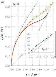
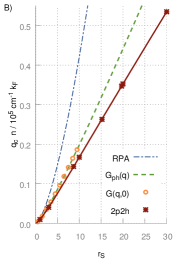
Figure 1: Plasmon dispersion (left) and critical wave vector (right) in different theories: bare RPA (dash-dotted blue lines), GRPA with $G_{\!\scriptscriptstyle\mathrm{ph}}(q)$ (dashed green lines) and with $G(q,0)$ [27] (orange short-dashed line (left) and, for a better distinction, orange circles (right)). The dark red results are from the dynamic pair theory of Sec. 3.

In Fig. 1 (left part) we compare $\omega_{\mathrm{pl}}(q)$ obtained with $G(q,0)$ and with $G_{\!\scriptscriptstyle\mathrm{ph}}(q)$ for $r_{\scriptscriptstyle\mathrm{S}}\!=\!10$. The agreement is amazing. The former approach uses $\omega\!=\!0$ data to describe an $\omega\!\gg qv_{\scriptscriptstyle\mathrm{F}}$ mode, while the latter is based on the $\omega-$integrated excitations to describe a single point $\omega_{\mathrm{pl}}(q)$. The inset shows the plasmon dispersion with RPA as well as $G_{\!\scriptscriptstyle\mathrm{ph}}(q)$ for $r_{\scriptscriptstyle\mathrm{S}}\!=\!1$. In this density regime, theories beyond RPA does not show much improvement. The critical wave vectors $q_{c}$ for Landau damping, again, almost coincide for all densities (where $G(q,0)$ is available). In the $G_{\!\scriptscriptstyle\mathrm{ph}}(q)$ approach $q_{c}$ measured in $k_{\scriptscriptstyle\mathrm{F}}=\sqrt{2\,\pi\,n}\,$ flattens around $2k_{\scriptscriptstyle\mathrm{F}}$ for large $r_{\scriptscriptstyle\mathrm{S}}$ (equivalent to a linear slope the units chosen).

Certainly, local field corrections massively lower the plasmon dispersion from its bare RPA value (blue lines in Fig. 1). Finite $T$ and $L$ effects, acting in different directions [26], cannot be expected to cancel the combined many-body correlations for all $(r_{\scriptscriptstyle\mathrm{S}},q)-$combinations.

The dispersion and thus $q_{c}$ are further significantly lowered by dynamic correlations (dark red lines in the figure). We therefore discuss the underlying theory next.

3 Dynamic Many Body Theory

All (static G)RPA approaches, Eqs. (3)–(2c), give no plasmon broadening outside the PHB. Scattering by impurities and phonons is beyond the jellium model; the lifetime $\tau\!\equiv\!\gamma^{-1}$ is often treated via replacing $\chi^{0}(q,\omega)\to\chi^{0\gamma}(q,\,\omega,\,i\gamma)$ (Lindhard-Mermin function [38]). A significant group of dynamic LFCs are of the so–called “quantum STLS” type [13]. In 3D these approaches describe the plasmon poorly [39], yielding $\mathrm{Im}\,\epsilon\propto-q^{5}/\omega^{7}$ near $\omega_{\mathrm{pl}}$ instead of the exact $+q^{2}/\omega^{11/2}$. We therefore refrain from discussing these theories further. (We are not aware of an analogous analytic 2D investigation, for a thorough numerical study, including finite width and finite $T$ effects, see [40]. These authors also study the dilute 2DEL in coupled bilayers [41].).

Intrinsic damping via multi–pair excitations requires a $q-$dependent lifetime and intricate response functions. A cornerstone, treating dynamic correlations, was presented by Neilson et al. [42]. Their density response function has the formal structure

$$\chi^{\scriptscriptstyle\mathrm{NSSS}}\;=\;\frac{\chi^{0\gamma}}{1-\big{[}V_{\!{}_{\mathrm{ph}}}-\frac{m\omega}{q^{2}}\,(\gamma\!-\!\gamma^{\mathrm{s}})\big{]}\,\chi^{0\gamma}}\;,$$ (15a)

$$\epsilon^{\scriptscriptstyle\mathrm{NSSS}}=\,1\!-\frac{v\,\chi^{0\gamma}}{1+\big{[}G_{\!{}_{\mathrm{ph}}}\!-\frac{m\omega}{\omega^{2}_{0}(q)}(\gamma\!-\!\gamma^{\mathrm{s}})\big{]}\,v\,\chi^{0\gamma}}\;,$$ (15b)

where $\gamma(q,\omega)$ is a mode-mode coupling memory function and $\chi^{0\gamma}$ is the Lindhard-Mermin function with the constant $\gamma$ replaced by the ,,self-motion” function $\gamma^{\mathrm{s}}(q,\omega)$.

The Dynamic Many Body Theory [23] accounts for correlated 2-particle – 2-hole (2p2h) excitations. Its strength lies in incorporating the best available static properties while determining the dynamic correlations via optimization. The derivation is sketched in A  and yields

$$\chi^{\scriptscriptstyle\mathrm{2p2h}}\;=\;\frac{\Pi_{\mathrm{s}}}{1-\big{[}V_{\!{}_{\mathrm{ph}}}+V_{\!{}_{\mathrm{2p2h}}}\big{]}\,\Pi_{\mathrm{s}}}\;,$$ (16a)

$$V_{\!{}_{\mathrm{2p2h}}}\>=\>\textstyle\frac{1}{4}\big{(}\frac{1}{S^{2}}\!-\!\frac{1}{{S^{0}}^{2}}\big{)}\,\displaystyle\big{(}W^{\scriptscriptstyle+}_{\mathrm{s}}\!+\!W^{\scriptscriptstyle-}_{\mathrm{s}}\big{)}\;,$$ (16b)

and

$$\epsilon^{\scriptscriptstyle\mathrm{2p2h}}=\,1\!-\frac{v\,\Pi_{\mathrm{s}}}{1+\big{[}G_{\!{}_{\mathrm{ph}}\!}+G_{\!{}_{\mathrm{2p2h\!}}}\big{]}\,v\,\Pi_{\mathrm{s}}}\;,$$ (16c)

$$\phantom{\Big{|}^{|}}\hskip 22.76228ptG_{\!{}_{\mathrm{2p2h\!}}}=\>\big{(}G^{0}_{\!{}_{\mathrm{ph}}\!}\!-\!1\big{)}\textstyle\frac{m}{\hbar^{2}q^{2}}\displaystyle\big{(}W^{\scriptscriptstyle+}_{\mathrm{s}}\!+\!W^{\scriptscriptstyle-}_{\mathrm{s}}\big{)}\;.\phantom{\bigg{|}_{|}}$$ (16d)

The ‘single–particle polarizability’ $\>\Pi_{\mathrm{s}}\!=\Pi_{\mathrm{s}}^{\scriptscriptstyle+}\!+\!\Pi_{\mathrm{s}}^{\scriptscriptstyle-}\>$ with

$$\Pi_{\mathrm{s}}^{\scriptscriptstyle\pm}\>=\>\frac{\chi^{0\scriptscriptstyle\pm}}{1-W^{\scriptscriptstyle\pm}_{\mathrm{s}}\chi^{0\scriptscriptstyle\pm}}\;,$$ (17a)

$$\vspace{-0.0cm}W^{\scriptscriptstyle\pm}_{\mathrm{s}}=\>\textstyle\frac{1}{2}\big{(}1\!+\!\frac{S}{S^{0}}\big{)}\displaystyle W^{\scriptscriptstyle\pm}+\textstyle\frac{1}{2}\big{(}1\!-\!\frac{S}{S^{0}}\big{)}\displaystyle W^{\scriptscriptstyle\mp}\phantom{\Big{|}_{|}}$$ (17b)

builds on the absorption and emission parts of $\chi^{0}$,

$$\chi^{0\scriptscriptstyle\pm}(q,\omega)=\>\frac{1}{N}\!\sum_{h}\frac{n_{h}(1\!-\!n_{h+q})}{\hbar\,\omega\pm(\varepsilon_{h}\!-\!\varepsilon_{h+q})+i0^{+}}\;,$$ (18)

($h$ includes the spin index) and the dynamic interactions,

$$W^{\scriptscriptstyle\pm\!}(q,\omega)\>=\>\frac{1}{2N}\!\!\sum\limits_{\mathbf{q}^{\prime},\mathbf{q}^{\prime\prime}}\delta_{{\bf q},\,{\bf q}^{\prime}+{\bf q}^{\prime\prime}}\,\big{|}\bar{K}_{\mathbf{q},\mathbf{q^{\prime}},\mathbf{q^{\prime\prime}}}\big{|}^{2}\,\mu^{\scriptscriptstyle\pm\!}(q^{\prime},q^{\prime\prime},\omega)\;.$$ (19)

We will no longer spell out the momentum conservation (but use ${\bf q}^{\prime\prime}$ as abbreviation for ${\bf q}\!+\!{\bf q^{\prime}}$). The pair propagator has, again, a mode-mode coupling structure: Its absorption part $\mu^{\scriptscriptstyle+}$ (an analogous form holds for $\mu^{\scriptscriptstyle-}$) is

$$\mu^{\scriptscriptstyle+\!}(q^{\prime},q^{\prime\prime},\omega)\>=\>-\!\int\limits_{-\infty}^{\infty}\!\!\frac{\mathrm{d}\hbar\omega^{\prime}}{2\pi i}\;\varkappa^{\scriptscriptstyle+\!}(q^{\prime},\omega^{\prime})\,\varkappa^{\scriptscriptstyle+\!}(q^{\prime\prime},\omega\!-\!\omega^{\prime})\;,$$ (20)

with

$$\varkappa^{\scriptscriptstyle+}\>=\>\frac{\chi^{\scriptscriptstyle 0+}\,S^{2}}{{S^{0}}^{2}+\hbar\omega\,S^{0}SX\,\chi^{\scriptscriptstyle 0+}}\;.$$ (21)

The function $\varkappa^{\scriptscriptstyle+}\!+\!\varkappa^{\scriptscriptstyle-}$ closely resembles $\chi^{\scriptscriptstyle\mathrm{GRPA}}$. In particular, their $\omega^{0}-$ and $\omega^{1}-$moments agree and their collective modes are also well matched [23]. In the plasmon-pole approximation (PPA, also termed ‘collective approximation’) they are identical, see B, Eq. (52).

The non–nodal (quantum Ornstein-Zernike) function $X(q)$, Eq. (8b), is the main ingredient for the three–body vertex in the dynamic interactions (19), together with equilibrium triplet correlations $\bar{u}^{(3)}$ [23],

$$\begin{array}[]{lllll}\displaystyle\!\!\!\!\bar{K}_{\mathbf{q},\mathbf{q^{\prime}},\mathbf{q^{\prime\prime}}}&\displaystyle\!\!\!=\>\mbox{\small$\displaystyle\frac{\hbar^{2}}{2m}$}\,\Big{[}\,\mathbf{q}\!\cdot\!\mathbf{q}^{\prime}\,X(q^{\prime})\,+\,\mathbf{q}\!\cdot\!\mathbf{q}^{\prime\prime}\,X(q^{\prime\prime})\vspace{0.2cm}\\ &\displaystyle\hfill-\,\;q^{2}\;\bar{u}^{(3)}_{\mathbf{q},\mathbf{q^{\prime}},\mathbf{q^{\prime\prime}}}\,\Big{]}\>.\!\!\!\!\end{array}$$ (22)

4 Results of the 2p2h Theory

For very short-lived plasmons caution is in order [43] whether they are defined as the real part of the complex zero of $\epsilon(q,z)$ with $z\!\equiv\omega\!+\!i\Gamma/2$, or as the maximum of the loss function,

$$\phantom{\big{|}_{|}}\epsilon(q,\,z_{\mathrm{pl}}) =0\;,$$ (23a)

$$-\mathrm{Im}\,\epsilon^{-1}(q,\omega_{\mathrm{pl}}) \rightarrow\mathrm{max}\;.$$ (23b)

For comparing calculated plasmon positions $\omega_{\mathrm{pl}}(q)$ with HREELS and X-ray scattering data, Eq. (23b) is adequate. We computed the 2p2h results with the same compressibility-corrected fit of the QMC data [28] for $S(q)$ as our GRPA values above (cf. C).

Figure 2 shows the imaginary part of $\chi^{\scriptscriptstyle\mathrm{2p2h}}$ for a highly dilute 2DEL. Above the PHB the plasmon is visible as a strong, sharp mode, broadened by the pair-excitations continuum. Beyond the critical wave vector $q_{\mathrm{c}}$ the mode travels, highly Landau damped, through the PHB and regains strength near its lower edge, as is most clearly seen in the left part of Fig. 1 : the rather broad orange peak is at a much lower energy than the sharp $q\!\approx\!0.25k_{\scriptscriptstyle\mathrm{F}}$ plasmon (dark red line), and of much higher strength than the $q\!=\!0.5k_{\scriptscriptstyle\mathrm{F}}$ and $1k_{\scriptscriptstyle\mathrm{F}}$ plasmons damped by 2-pair excitations (dashed lines).

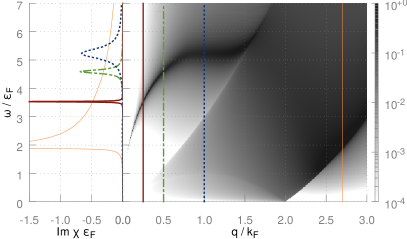
Figure 2: Scattering loss function -Im$\chi(q,\omega)$ (right, arbitrary values) together with cuts at 4 characteristic wave vectors $q_{i}$ (left) for a dilute 2DEL ($r_{\scriptscriptstyle\mathrm{S}}=20$) from the 2p2h theory. The line styles on the left agree with those marking these $q_{i}$ in the right part.

$r_{\mathrm{S_{\phantom{|}}}}$	2	5	10	20	30
$n_{\scriptscriptstyle\mathrm{GaAs}}$ $\left[10^{9}/\mathrm{cm}^{2}\right]$	75.2	12	3	0.75	0.33
$q_{\mathrm{c}}^{\scriptscriptstyle\mathrm{RPA}}\,\big{[}k_{\scriptscriptstyle\mathrm{F}}\big{]}$	1.50	2.45	3.55	5.09	6.28
$q_{\mathrm{c}}^{\scriptscriptstyle\mathrm{RPA}}\,[10^{5}/\mathrm{cm}]$	10.	6.8	4.9	3.5	2.9
$q_{\mathrm{c}}^{\scriptscriptstyle\mathrm{GRPA}}\,\big{[}k_{\scriptscriptstyle\mathrm{F}}\big{]}$, $\,G(q,0)$	1.13	1.47	1.70	–	–
$q_{\mathrm{c}}^{\scriptscriptstyle\mathrm{GRPA}}\,\big{[}k_{\scriptscriptstyle\mathrm{F}}\big{]}$, $\,G_{\scriptscriptstyle\mathrm{ph}}(q)$	1.28	1.54	1.77	1.93	2.00
$q_{\mathrm{c}}^{\scriptscriptstyle\mathrm{2p2h}}\,\big{[}k_{\scriptscriptstyle\mathrm{F}}\big{]}$	1.05	1.31	1.44	1.53	1.55
$q_{\mathrm{c}}^{\scriptscriptstyle\mathrm{2p2h}}\,[10^{5}/\mathrm{cm}]$	7.23	3.61	1.98	1.05	0.71

Table 1: Plasmon critical wave vector in reduced units and for a AlGaAs quantum well with areal density as given in the header. Upper two rows: bare RPA results. Middle two lines: Results from QMC based static local field corrections, Davoudi et al. [27] and Eq. (7). Lower two rows: results of this work.

In the static (G)RPA theories the critical wave vector $q_{\mathrm{c}}$ where the plasmon hits the PHB is given by the implicit equation

$$1+\,\frac{E_{\scriptscriptstyle\mathrm{F}}}{V_{\!\varepsilon}(q_{\mathrm{c}})}\>=\>\sqrt{1\!+\frac{2k_{\scriptscriptstyle\mathrm{F}}}{q_{\mathrm{c}}}}\;.$$ (24)

(Note that this also holds for layers of finite width). The $r_{\scriptscriptstyle\mathrm{S}}\!\to\!0$ (i.e.  high density) solution is given by the RPA as $q_{\mathrm{c}}\approx(2\,r_{\scriptscriptstyle\mathrm{S}})^{2/3\,}k_{\scriptscriptstyle\mathrm{F}}$. At intermediate densities, $r_{\scriptscriptstyle\mathrm{S}\!}\approx 1\ldots 5$, the two GRPA approaches and the dynamic pair theory yield comparable values, while $q_{\mathrm{c}}^{\scriptscriptstyle\mathrm{RPA}}$ is markedly too high ($>\!50\%$ at $r_{\scriptscriptstyle\mathrm{S}}\!=\!5$, see Tab. 1). For the highly dilute 2DELs of interest here, dynamic pair fluctuations flatten the plasmon dispersion (cf. Fig. 1) and, consequently, significantly lower $q_{\mathrm{c}}$ further. For densities with $r_{\scriptscriptstyle\mathrm{S}}\!\lesssim\!30$ the numerically obtained $q_{\mathrm{c}}^{\mathrm{2p2h}}$ can be accurately fitted by

$$q_{\mathrm{c}}^{\mathrm{2p2h}}(r_{\scriptscriptstyle\mathrm{S}})\>=\>\frac{(2\,r_{\scriptscriptstyle\mathrm{S}})^{2/3}+0.247117\,r_{\scriptscriptstyle\mathrm{S}}}{1+1.916638\,r_{\scriptscriptstyle\mathrm{S}}^{1/2}+0.290381\,r_{\scriptscriptstyle\mathrm{S}}}\,k_{\scriptscriptstyle\mathrm{F}}\;,$$ (25)

capturing both, $r_{\scriptscriptstyle\mathrm{S}}\!\to\!0$ as well as the nearly horizontal $q_{\mathrm{c}}^{\mathrm{2p2h}}\approx 1.5\,k_{\scriptscriptstyle\mathrm{F}}$ behavior for $r_{\scriptscriptstyle\mathrm{S}}\!\gtrsim\!20$. The comparison of the fit with the numerical results is shown in Fig. 1 (dark red line and markers, respectively).

In order to facilitate comparison with experiments or other theories, we next give an approximate analytic expression for the 2p2h plasmon dispersion obtained numerically from Eq. (23b). Finding a formula valid for a wide range in both $q$ and $r_{\scriptscriptstyle\mathrm{S}}$ is a formidable task. A Padé inspired expression with wave vectors measured in the critical $q_{\mathrm{c}}(r_{\scriptscriptstyle\mathrm{S}})$ given in Eq. (25) proved to work best. Denoting $\underline{q}\!\equiv\!q/q_{\mathrm{c}}$ and $\omega_{\mathrm{pl}}^{\mathrm{c}}\!\equiv\omega_{\mathrm{pl}}(q_{\mathrm{c}})$ the following ansatz with the Padé function of order $n\!+\!m$ fulfills the limit (14)

$$\omega^{\mathrm{fit}}_{\mathrm{pl}}\>=\>\omega_{\mathrm{pl}}^{\mathrm{c}}\,\sqrt{\underline{q}}\>P_{\!{}_{[n,m]\!}}\big{(}\underline{q},\,r_{\scriptscriptstyle\mathrm{S}}\big{)}\;,\phantom{\bigg{|}_{|}}$$ (26a)

$$P_{[n,m]}(\underline{q},r_{\mathrm{s}})\>=\>\frac{\sum_{i=0}^{n}\,p_{i}(r_{\scriptscriptstyle\mathrm{S}})\,\underline{q}^{i}}{1+\sum_{j=1}^{m}\,\tilde{p}_{j}(r_{\scriptscriptstyle\mathrm{S}})\,\underline{q}^{j}}\;.$$ (26b)

Details on the fitting procedure and the coefficients $p_{i}(r_{\scriptscriptstyle\mathrm{S}})$, $\tilde{p}_{j}(r_{\scriptscriptstyle\mathrm{S}})$ are given explicitly in D, Eq. (64), and Tab. 2. In the supplementary material we provide an implementation of our fit for several widely spread tools (Origin${}^{\text{\textregistered}}$,  MATLAB${}^{\text{\textregistered}}$, Mathematica${}^{\text{\textregistered}}$) plus another set of coefficients, specifically suited for ultra-low densities.

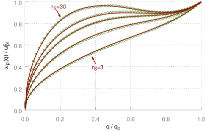
Figure 3: Plasmon dispersion from Eq. (26) (lines) compared to the numerical data (points) for the full validity range of the fit, in particular, $r_{\scriptscriptstyle\mathrm{S}}\!=\!3,\,8.7,\,15.2,\,19.7,30$. Increasing $r_{\mathrm{s}}$ corresponds to higher dispersions. The values $r_{\scriptscriptstyle\mathrm{S}}=8.7,\,15.2$ and $19.7$ were reported for the AlGaAs quantum well in [19].

As seen in Fig. 3, the dispersion given in Eq. (26a) accurately reproduces the numerical data over the wide density range of $r_{\scriptscriptstyle\mathrm{S}}\!\in[3,30]$. To ease comparison, all $\omega_{\mathrm{pl}}(q)$ were normalized to $\omega^{\mathrm{c}}_{\mathrm{pl}}$. For small $q$ and in the vicinity of $q_{\mathrm{c}}$ the error is well below 1% and never exceeds 2%.

In bulk systems, multi–pair damping is negligible compared to other sources, the contribution to the life-time’s dispersion, however, is significant [44]. We now investigate the sheet plasmon width and the $q-$dependence of the 2p2h plasmon peak. In its vicinity $\mathrm{Im}\chi^{\scriptscriptstyle\mathrm{2p2h}}(q,\omega)$ is well represented by a Lorentzian,

$$-\mathrm{Im}\chi^{\scriptscriptstyle\mathrm{2p2h}}(q,\omega)\;\approx\;\frac{\Gamma_{\!\scriptscriptstyle\mathrm{2p2h}}(q)/\pi}{\big{(}\omega\!-\!\omega^{\mathrm{2p2h}}_{\mathrm{pl}}(q)\big{)}^{2}\,+\,\Gamma^{2}_{\!\scriptscriptstyle\mathrm{2p2h}}(q)}\,,$$ (27)

confirmed both analyically as well as by fitting the numerically obtained $\mathrm{Im}\chi^{\scriptscriptstyle\mathrm{2p2h}}(q,\omega)$ (see Fig. 4). Unless very close to the Landau damping region, the agreement of $\Gamma_{\!\scriptscriptstyle\mathrm{2p2h}}$ with the true FWHM is excellent.

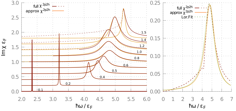
Figure 4: Full 2p2h loss function (dark red) and Lorentzian plasmon peak (orange) at $r_{\scriptscriptstyle\mathrm{S}}\!=20$. Left: Spectra for $q/k_{\scriptscriptstyle\mathrm{F}}$ as indicated, shifted by 0.2$\varepsilon_{\scriptscriptstyle\mathrm{F}}$ for better visibility. Full (dashed) lines hold outside (inside) the particle–hole band (note the asymmetry in $\omega$ near $q\!\approx\!q_{\mathrm{c}}$). Right: Close up for $q\!=\!1.3k_{\scriptscriptstyle\mathrm{F}}\!=0.85q_{\mathrm{c}}$: numerical (short-dashed), approximate (dotted) and fitted (full) curves.

The fit for $\Gamma_{\!\scriptscriptstyle\mathrm{2p2h}}(q;r_{\scriptscriptstyle\mathrm{S}})$ is given in the supplementary material (Eq. (LABEL:S-Seq:_lifetime_fit) with the coefficients of table LABEL:S-STab:_FWHMfit), where we also compare the width-dispersion $\Gamma_{\!\scriptscriptstyle\mathrm{2p2h}}(q)$ with experimental values. Similar to the bulk, this intrinsic damping is negligible compared to that caused by ‘external’ mechanisms (phonon and impurity scattering, inter-subband excitations, etc.). In contrast to 3D [44], however, adding $\Gamma(q\!=\!0)$ (either from experiment or theories beyond the electron liquid) to $\Gamma_{\!\scriptscriptstyle\mathrm{2p2h}}(q)$, does not explain the observations here.

5 Plasmon dispersion in semiconductor QWs

5.1 Comparison with the classical dispersion

A common method for determining the electron density from diffraction measurements is to fit the experimental plasmon dispersion to an RPA-like form. As discussed, the bare RPA (Eq. (11) with $V_{\!\epsilon}(q)\!\to\!v(q)$), underestimating correlations, grossly overestimates $\omega_{\mathrm{pl}}(q)$. Static correlations, further augmented by dynamic ones, act in the opposite direction. Temperature effects raise $\omega_{\mathrm{pl}}(q)$, while increasing the layer width softens it [26, 45]: The smeared out wave function $\varphi_{\!\scriptscriptstyle 0}(z)$ of the quantum well reduces the effective interaction and thus lowers the RPA correlations (approaching the bulk result for very wide wells would require to account for multiple subbands).

Obviously, comparing theory with measurements would require a precise, independent experimental determination of more parameters than possible.

Specifically, $r_{\scriptscriptstyle\mathrm{S}}$ (i.e. the areal electron density $n$) is subject to some ambiguity [26]. In [19] it was determined from fitting the plasmon dispersion to the empirical form

$$\omega^{\mathrm{exp}}_{\mathrm{pl}}(q)\>=\>\omega_{0}(q)\,\sqrt{1+q\,\xi\,}\;,$$ (28)

where the length $\xi$ contains all effects due to temperature $T$, well-width $L$, and correlations; the latter, in turn, are split into RPA ($\equiv$ ‘non-local’) and LFC contributions,

$$\xi\!\equiv\xi^{L,T}_{\,\mathrm{tot}} \equiv\>\xi^{0,0}_{\mathrm{tot}}+\xi^{0,T}-\xi^{L,0}\;,$$ (29a)

$$\xi^{0,0}_{\mathrm{tot}} =\big{(}\xi^{\scriptscriptstyle\mathrm{RPA}}_{\mathrm{cor}}-\xi^{\scriptscriptstyle\mathrm{LFC}}_{\mathrm{cor}}\big{)}^{\!0,0}\,\equiv\>+\xi_{\mathrm{nloc}}^{0,0}-\xi_{\mathrm{cor}}^{0,0}\;.$$ (29b)

(see E about terminology). For very low temperatures the observed $\xi$ scales with $k_{\scriptscriptstyle\mathrm{F}}^{-1}$; since in the 2DEG $\xi_{\mathrm{nloc}}$ is density–independent, the zero temperature limit is interpreted [19] as the correlation part

$$\xi_{\mathrm{exp}}\xrightarrow[\to 0]{T}\>-(0.17\!\pm\!0.04)\,\sqrt{2}/k_{\scriptscriptstyle\mathrm{F}}\>\equiv\>-\xi^{L,0}_{\,\mathrm{cor}}(r_{\scriptscriptstyle\mathrm{S}})\Big{|}_{\mathrm{exp}}\;.$$ (30)

The RPA term $\xi^{\scriptscriptstyle 0,0}_{\mathrm{nloc}}=3a_{\scriptscriptstyle\rm B}^{*}/8$ follows from Eq. (12) with $V_{\!\epsilon}(q)\!\to\!v(q)$. From the small $q$ expansion of Eq. (26)) we here provide a state-of-the-art result for the correlation coefficient due to two-pair excitations in the strictly 2DEL:

$$-\xi^{0,0}_{\,\mathrm{cor}}(r_{\scriptscriptstyle\mathrm{S}})\Big{|}_{\mathrm{2p2h}}\>=\>\frac{2}{q_{\mathrm{c}}(r_{\scriptscriptstyle\mathrm{S}})}\,\Big{(}\frac{p_{1}}{p_{0}}-\tilde{p}_{1}\Big{)}\,-\frac{3}{8}\,a_{\scriptscriptstyle\rm B}^{*}\;.$$ (31)

In Fig. 5  this is compared with $\xi^{L,0}_{\,\mathrm{cor}}$ determined from Eq. (30). As expected, the computed strictly 2D correlation effects are larger in magnitude than those measured for $L\!\approx 330$Å.

In a QW with lowest subband wave function $\varphi_{\!\scriptscriptstyle 0}$ the 3D density $\rho({\bf r},z)$ can often be approximated as $n\,|\varphi_{\!\scriptscriptstyle 0}(z)|^{2}$. The 2D Coulomb potential is then modified with an $r_{\scriptscriptstyle\mathrm{S}}-$independent ‘form factor’ $F(q)$,

$$v(q) \to v(q)\,F(q)$$ (32a)

$$F(q) =\int\!\!dz_{1}\!\int\!\!dz_{2}\>\big{|}\varphi_{{}_{0\!}}(z_{1})\big{|}^{2}\,e^{-q|z_{1}-z_{2}|}\,\big{|}\varphi_{{}_{0\!}}(z_{2})\big{|}^{2}\;.$$ (32b)

Clearly, this yields a density-independent dispersion coefficient $\xi^{L,0}$, where

$$F(q\!\to\!0) =1-q\,\xi^{L,0}\;;\quad\xi^{L,0}\!>\!0\phantom{\Big{|}_{|}}$$ (33a)

$$\omega^{L,0\!}_{\mathrm{pl}}(q\!\to\!0)\Big{|}_{\scriptscriptstyle\mathrm{RPA}} =\>\omega_{0}(q)\,\sqrt{1+\big{(}\textstyle\frac{3}{8}\displaystyle a_{\scriptscriptstyle\rm B}^{*}-\xi^{L,0}\big{)}\,q\,}\;.$$ (33b)

The full RPA finite $L$ plasmon is given by $V_{\!\epsilon}\to vF$ in Eq. (12) (cf. F for details).

While both these contributions to the plasmon dispersion are constant, the LFC part must increase with $r_{\scriptscriptstyle\mathrm{S}}$. Since correlations are the stronger the thinner the QW and/or the higher $r_{\scriptscriptstyle\mathrm{S}}$, the discrepancy in Fig. 5 increases for dilute systems. Cum grano salis, the computed $L\!=\!0,\,T\!=\!0$ data presented in the figure can thus be considered as a lower bound for measurements.

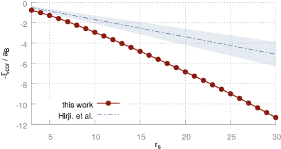
Figure 5: Plasmon correlation wavelength $\xi^{\scriptscriptstyle 0,0}_{\mathrm{cor}}$ from the 2p2h theory for a strictly 2DEL (solid line: fit (26), markers: numerical data) and measured estimate for a finite width AlGaAs 2DEL [19] (double-dashed line with shaded error bar).

We next turn to incorporating finite $L$ and finite $T$ effects into our approach. The static GRPA theories of Sec. 2 both rely on equilibrium QMC results, one needing $G(q,\omega;\,L\!=\!0,T\!=\!0)$, the other $S(q;\,L\!=\!0,T\!=\!0)$. The latter function is also input to the 2p2h theory. No QMC results for $G(q,0;L,T)$ and $S(q;L,T)$ are available. For the plasmon we therefore adopt the above intuitive strategy,

$$\omega^{L,T\!}_{\mathrm{pl}}(q;r_{\scriptscriptstyle\mathrm{S}})\>=\>\omega^{0,0\!}_{\mathrm{pl}}(q,r_{\scriptscriptstyle\mathrm{S}})\,\sqrt{1+\big{(}\xi^{0,T\!}(r_{\scriptscriptstyle\mathrm{S}})\!-\!\xi^{L,0}\big{)}\,q\,}.\;$$ (34)

The parameters $\xi^{\scriptscriptstyle 0,T}$ and $\xi^{\scriptscriptstyle L,0}$ are taken from the experiment under consideration, $\omega^{0,0\!}_{\mathrm{pl}}$ from the fit (26) of the 2p2h result. For long wavelengths (34) is exact and identical to

$$\omega_{0}\,\sqrt{1+\big{(}\xi^{0,0\!}_{\mathrm{tot}}(r_{\scriptscriptstyle\mathrm{S}})\!+\!\xi^{0,T}(r_{\scriptscriptstyle\mathrm{S}})\!-\!\xi^{L,0}\big{)}\,q\,},\;$$ (35)

(with the classical $\omega_{0}\propto\!\sqrt{q}/r_{\scriptscriptstyle\mathrm{S}}$ and notation as in Eq. (29)).

5.2 Application: electron density

We apply this to the $L\!=\!330$Å GaAs QW experimentally studied at $T\!=1.85K$ in [19, 20]. There, two samples were fitted to the empirical form (28), resulting in $r_{\scriptscriptstyle\mathrm{S}}\!=8.7$ and $19.7$, respectively (full thin blue lines in Fig. 6). Taking $\xi^{0,T}$ from Fig. 4 of [19], a least square fit of (34) yields the somewhat different values $r_{\scriptscriptstyle\mathrm{S}}\!=8.22$ ($n\approx 4.46\!\times\!10^{9}\mathrm{cm^{-2}}$) and $16.25$ ($n\approx 1.14\!\times\!10^{9}\mathrm{cm^{-2}}$) (full thick red lines in Fig. 6). For the denser sample (left panel), theory and experiment agree nicely; with an $r_{\scriptscriptstyle\mathrm{S}}-$difference of $\sim\!5$%.

The ultra-dilute case (where $r_{\scriptscriptstyle\mathrm{S}}$ differs by 15%) is less satisfactory, the 2p2h curve being too flat compared to the experiment. Conversely, in 2D ³He [46] dynamic pair correlations proved crucial to explain the measured spectrum. At a density of $1/a^{2}\pi\!\approx\!10^{9}\,\mathrm{cm}^{-2}$, the plasmon with $q\!=0.7\!\times\!10^{5}\,\mathrm{cm}^{-1}$ has a wavelength of $\lambda\!=2\pi/q\!\approx\!5a$ and thus definitely should ‘feel’ the two–body fluctuations. We attribute the discrepancy to the fact that the width $L$ not only diminishes the RPA $q\!\to\!0$ dispersion, but reduces correlations in general. Since larger $q$ are more affected by correlation effects, their reduction will also be larger there, diminishing the negative curvature of $\omega^{\scriptscriptstyle\mathrm{2p2h}\!}_{\mathrm{pl}}(q)$ (see F for further details).

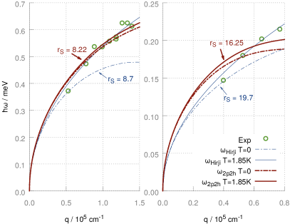
Figure 6: Measured plasmon energies (green dots) for two samples, fitted to Eq. (28), including both, finite temperature and finite width dispersion (blue solid lines), and for $\xi^{\scriptscriptstyle 0,T\!}\!=\!0\!=\!\xi^{\scriptscriptstyle L,0}$ (dashed–dotted blue lines) [19]. Dark-red dispersions: fit of the theoretical 2p2h results (34) to the experimental data, again with and without $\xi^{\scriptscriptstyle 0,T\!},\,\xi^{\scriptscriptstyle L,0}$ (solid and dashed–dotted lines, respectively).

6 Conclusions

We calculated the excitation spectrum of the 2DEL including 2p2h excitations, with special emphasis on the application to AlGaAs QWs. We found that dynamic pair correlations lower the sheet plasmon’s dispersion massively. The agreement with experiments is good, except for ultra-dilute sytems, where finite width effects should be better accounted for. This requires the availability of high-quality data for the $L\!\neq\!0$ pair distribution function; work in this direction is in progress. For zero well width we provided a fit of the plasmon dispersion $\omega^{\scriptscriptstyle\mathrm{2p2h}\!}_{\mathrm{pl}}(q;r_{\scriptscriptstyle\mathrm{S}})$, valid in the whole range of $r_{\scriptscriptstyle\mathrm{S}}\!\in[3,\ldots,30]$ and $q\in[0,\ldots,q_{\mathrm{c}}]$ (see download in the Supplementary Material).

An extension of the dynamic pair theory to spin-dependent effective dynamic interactions in partially spin–polarized 2DELs [47] appears of practical interest, due to the low–loss attribute of the magnetic antiresonance [32]. The input functions needed for such systems are available for $L\!=\!0$ [28] and currently studied in our group for $L\!\neq\!0$. Another topic worth pursuing is the influence of dynamic correlations on the effective mass enhancement [48, 49, 50].

Appendix A 2-Pair Fluctuations

Our approach extends the widely used Jastrow-Feenberg ansatz for a many–particle ground state to excited states [51, 52]. Both share the advantage of avoiding the summation of many, mutually cancelling diagrams by obtaining the correlations via an optimization procedure.

The ground state wave function is approximated as

$$|\Psi_{\rm g}\rangle\>=\>\textstyle\frac{1}{{\cal I}^{1/2}_{\!\rm g}}\;\displaystyle\exp\!\big{(}\overline{U}_{\!\rm g}\big{)}\>|\Phi_{\!{}_{0}}\rangle\;,$$ (36)

(${\cal I}_{\!\rm g}$ is the normalization integral, $\Phi_{\!{}_{0}}$ a Slater–determinant). The correlation operator [51] $\,\mathrm{exp}(\overline{U}_{\!\rm g})$ invokes n-body equilibrium correlation functions $\bar{u}_{n}({\bf r}_{1},\ldots,{\bf r}_{n})$

$$\overline{U}_{\!\rm g}\equiv\>\textstyle\frac{1}{2}\displaystyle\!\sum_{\scriptscriptstyle i<j}\bar{u}_{2}(|{\bf r}_{i}\!-\!{\bf r}_{j}|)\>+\textstyle\frac{1}{2}\displaystyle\!\!\sum_{\scriptscriptstyle i<j<k\!}\bar{u}_{3}({\bf r}_{i},{\bf r}_{j},{\bf r}_{k})\>+\>\ldots\;,$$ (37)

obtained optimally from minimizing the energy $E_{\rm g}$. This focuses right away on the comparably small correlations, avoiding the summation of large perturbational terms with opposite sign.

The Dynamic Many Body Theory [24, 23, 46, 52] generalizes this idea to a system perturbed by $H_{\rm ext}(t)$ (the full Hamiltonian is $\,\widehat{H}_{\rm tot}\!=\widehat{H}\!+\!\widehat{H}_{\rm ext}$). The perturbed wave function takes a form analogous to Eq. (36):

$$|\Psi(t)\rangle\>=\>\textstyle\frac{1}{{\cal I}^{1/2}_{\!t}}\displaystyle\;\exp\!\big{(}\overline{U}_{\!\rm g}\big{)}\>\exp\!\big{(}\widehat{U}_{t}\big{)}\>|\Phi_{\!{}_{0}}\rangle\;$$ (38)

(again, ${\cal I}_{t}$ ensures the normalization). We abbreviate $k\!\equiv({\bf k},\sigma_{\!\scriptscriptstyle k})$ for wave vector and spin. The excitation operator reads

$$\widehat{U}_{t} \equiv -\textstyle\frac{it}{\hbar}\displaystyle E_{\rm g}\,+\sum_{\scriptscriptstyle p_{1}h_{1}}u^{(1)}_{p_{1}h_{1}\!}(t)\;a^{\dagger}_{p_{1}\!}a^{\phantom{\dagger}}_{h_{1}}$$

$$+ \sum_{\scriptscriptstyle p_{1}\!h_{1}p_{2}h_{2}}\!\textstyle{1\over 2}\displaystyle u^{(2)}_{p_{1}h_{1}p_{2}h_{2}\!}(t)\;a^{\dagger}_{p_{1}\!}a^{\phantom{\dagger}}_{h_{1}}\,a^{\dagger}_{p_{2}\!}a^{\phantom{\dagger}}_{h_{2}}\phantom{\bigg{|}^{|}}\;.$$

It creates $n$-particle – $n$-hole excitations ($n\!=\!1,2$) from the free determinant $|\Phi_{\!{}_{0}}\rangle$, dynamically coupled by the “$n$-pair–fluctuations” $u^{\scriptscriptstyle(n)}_{\scriptscriptstyle p_{1}\ldots h_{n}}$, finally correlated by $\overline{U}_{\!\rm g}$. The fluctuations are again determined via functional optimization (‘least’ action principle).

The deviations $\delta A\!\equiv\langle\widehat{A}\!-\!A_{\rm g}\rangle$ of an observable $\widehat{A}$ from its unperturbed value $A_{\rm g}$ are now calculated with the wave function (38). In linear response, only first order terms in $u^{(n)}$ need to be kept. This results in a sum over $n-$pair fluctuations weighted with matrix elements,

$$\delta A=\>{\Re}e\sum_{n=1}^{2}\textstyle\frac{1}{n!}\displaystyle\!\!\sum_{p_{1}\ldots h_{n}}\overline{\cal A}_{0,\,p_{1}\ldots h_{n}}\>u^{(n)}_{p_{1}\ldots h_{n}}\,.$$ (40)

The transition integrals $\overline{\cal A}_{0,\,p_{1}\ldots h_{n}}$ involve, due to $\delta\widehat{U}$ in (A), $n-$pair excited states,

$$|\Phi_{p_{1}\ldots h_{n}}\rangle\equiv\>\exp\!\big{(}\overline{U}_{\!\rm g}\big{)}\>a^{\dagger}_{p_{1}\!}a^{\phantom{\dagger}}_{h_{1}}\!\ldots a^{\dagger}_{p_{n}\!}a^{\phantom{\dagger}}_{h_{n}}\,|\Phi_{\!{}_{0}}\rangle\;.$$ (41)

These form a complete but not orthogonal set (c.f. the “correlated basis functions” in [31]). We denote the plain overlaps, i.e. those of $\delta\widehat{A}\!=\!1$, as $\overline{\cal N}_{\!0,\,p_{1}\ldots h_{n}}$. Evaluating these high-dimensional integrals is rather uneconomical. Much more promising is a localization strategy.

A prime example involves the static structure factor,

$$S(q)\>\equiv\>\langle\delta\widehat{\rho}_{\bf q}\,\delta\widehat{\rho}_{-\bf q}\rangle/N\;.$$ (42)

Expressing the density fluctuations via creation– and annihilation operators and applying $\delta\widehat{\rho}_{\bf q}\delta\widehat{\rho}_{-\bf q}$ to $|\Psi_{\!\rm g}\rangle$ leads to

$$S(q)\>=\>S^{0}(q)+\>\textstyle\frac{1}{N}\displaystyle\!\sum_{h_{1}h_{2}}\overline{\cal N}_{\!0,\,p_{1}h_{1}p_{2}h_{2}}\,,\;\mbox{\footnotesize$\begin{array}[]{ccc}{\bf p_{1}}\equiv{\bf h_{1}}\!-\!{\bf q}\\ {\bf p_{2}}\equiv{\bf h_{2}}\!+\!{\bf q}\end{array}$}\;,$$ (43)

with the free structure factor $S^{0}(q)$ [13]. Knowledge of $S(q)$ from any state-of-the-art theory can therefore be used to replace the $h_{i}-$summed $\overline{\cal N}_{\!0,\,p_{1}\ldots h_{2}}\,$. This example captures the idea: Unknown non-local matrix elements $\,\overline{\cal A}\,$ are approximated by known local functions ${\cal A}_{\scriptscriptstyle\rm av}^{\scriptscriptstyle(\ell,n)}$, depending only on the transferred momenta:

$$\overline{\cal A}_{p^{\prime}_{1}\ldots h^{\prime}_{\ell},\,p_{1}^{\phantom{,\!}}\ldots h_{n}^{\phantom{,\!}}}\>\longrightarrow\;{\cal A}_{\scriptscriptstyle\rm av}^{\scriptscriptstyle(\ell,n)}(\mbox{\small${\bf q}^{\prime}_{1},\ldots,{\bf q}_{n-1}^{\phantom{,\!}}$})\,,\;\mbox{\footnotesize$\begin{array}[]{ccc}{\bf q_{i}}\equiv{\bf p_{i}}\!-\!{\bf h_{i}}\\ {\bf q_{i}^{\prime}}\equiv{\bf p_{i}^{\prime}}\!-\!{\bf h_{i}^{\prime}}\end{array}$}\qquad$$ (44)

(momentum conservation implies that the sum of all ${\bf q}_{i}$ equals that of all ${\bf q}^{\prime}_{i}$). For the ground state quantities ${\cal A}_{\scriptscriptstyle\rm av}^{\scriptscriptstyle(\ell,n)}$ the best available data (e.g. $S(q)$ from QMC simulations [28]) are taken.

The density response follows from Eq. (40) as

$$\delta\rho({\bf q};t) = {\Re}e\bigg{\{}\sum_{p_{1}^{\prime}\ldots h_{1}}\overline{\cal N}_{\!p^{\prime}_{1}h^{\prime}_{1},\,p_{1}^{\phantom{{}^{\prime}}}h_{1}^{\phantom{{}^{\prime}}}}\>u^{(1)}_{p_{1}h_{1}\!}(t)\>+\>$$

$$\sum_{p_{1}^{\prime}\ldots h_{2}}\overline{\cal N}_{\!p^{\prime}_{1}h^{\prime}_{1},\,p_{1}^{\phantom{{}^{\prime}}}h_{1}^{\phantom{{}^{\prime}}}p_{2}^{\phantom{{}^{\prime}}}h_{2}^{\phantom{{}^{\prime}}}}\>\textstyle\frac{1}{2}\displaystyle u^{(2)}_{p_{1}h_{1}p_{2}h_{2}\!}(t)\bigg{\}}\;.$$

The local approximations of the $\overline{\cal N}-$matrices are all closely related to the ground state $n-$particle structure factors [23]. Next, the fluctuation amplitudes $u^{(1)},\,u^{(2)}$ are determined from Euler–Lagrange equations (EL-eqs).

The Lagrangian corresponding to Schrödinger’s equation and the ansatz (38) give

$${\cal L}(t)=\>\langle\Psi(t)\big{|}\,\widehat{H}_{\rm tot}\!-i\hbar\frac{\partial}{\partial t}\,\big{|}\Psi(t)\rangle\;,$$ (46a)

$$\bigg{(}\,\mbox{\small$\displaystyle\frac{\delta}{\delta u^{*(n)}_{p_{1}\ldots h_{n}}}\,-\,\frac{d}{dt}\frac{\delta}{\delta\dot{u}^{*(n)}_{p_{1}\ldots h_{n}}}$}\,\bigg{)}\,{\cal L}(t)\>=\>0\;.$$ (46b)

For excitation operators of the type (A) the time derivative term yields for the lhs of (46b)

$$\textstyle\frac{i\hbar}{{\cal I}_{\!t}}\displaystyle\big{\langle}e^{\overline{U}_{\!\mathrm{g}}}e^{\widehat{U}^{\dagger}_{t}}a^{\dagger}_{p_{1}}\!\ldots a^{\phantom{\dagger}}_{h_{n}}\!\Phi_{\!{}_{0}}\,\big{|}\big{(}1\!-\!|\Psi\rangle\langle\Psi|\big{)}\big{|}\,e^{\overline{U}_{\!\mathrm{g}}}e^{\widehat{U}^{\dagger}_{t}}\,\widehat{\dot{U}}_{\!t\,}\Phi_{\!{}_{0}}\big{\rangle}.$$ (47)

In linear response this invokes the $\dot{u}^{(n)}_{p_{1}\ldots h_{n}}$ and the $\overline{\cal N}$-matrix elements of Eq. (A). Due to

$$\widehat{H}_{\rm ext}=\int\!\!d^{2}r\>V_{\!\rm ext}({\bf r},t)\,\widehat{\rho}({\bf r})\;,$$ (48)

these also enter the perturbation contribution of (46).

The remaining, essential parts of the EL-eqs arise from $\langle\Psi(t)|\widehat{H}|\Psi(t)\rangle$. We first take the functional derivative and then calculate the expectation value in linear response as outlined above, now for the operator $\widehat{A}\to a^{\dagger}_{p_{1}\!}\ldots a_{h_{n}}^{\phantom{{}^{\prime}}}\widehat{H}$. This brings the transition integrals of the Hamiltonian into play:

$$\overline{\cal H}_{p_{1}^{\phantom{{}^{\prime}}}\ldots h_{n}^{\phantom{{}^{\prime}}},p_{1}^{\prime}\ldots h_{n}^{\prime}}\quad\mbox{and}\quad\overline{\cal H}_{0,\,p_{1}\ldots h_{n}^{\phantom{{}^{\prime}}}}\;.$$ (49)

For $\widehat{H}_{\mathrm{ext}}\!=\!0$ the EL-eqs must be fulfilled with $\widehat{U}_{t}\!=\!0$ (equilibrium condition). From this the optimal local functions ${\cal H}_{\scriptscriptstyle\rm av}^{\scriptscriptstyle(\ell,n)}$ are determined in the spirit discussed above. With $t_{k}\!\equiv\hbar^{2}k^{2}/2m$, end up with the diagonal and off-diagonal Hamiltonian matrix elements approximated as

$$\begin{array}[]{rlllll}\displaystyle\overline{\cal H}_{p_{1}\ldots h_{n},p_{1}\ldots h_{n}}\!\rightarrow&\!\!\!\sum_{i=1}^{n}\big{(}t_{p_{i}}\!-t_{h_{i}}\big{)}\equiv\sum_{i=1}^{n}e_{p_{i},h_{i}}\;,\vspace{0.3cm}\\ \displaystyle\overline{\cal H}_{p_{1}^{\phantom{{}^{\prime}}}\ldots h_{n}^{\phantom{{}^{\prime}}},p_{1}^{\prime}\ldots h_{n}^{\prime}}\!\rightarrow&\!\!\!\!\frac{1}{2}\!\sum_{i=1}^{\scriptscriptstyle n+n^{\prime}\!}\big{(}e_{p_{i},h_{i}}\!-\textstyle\frac{t_{q_{i}}}{S^{0}(q_{i})}\displaystyle\big{)}\,{\cal N}_{\scriptscriptstyle\rm av\!}(\mbox{\footnotesize${\bf q_{1}},\ldots,{\bf q_{n}^{\prime}}$})\,,\end{array}$$ (50)

respectively. Here, the 2p2h-part $\overline{\cal H}_{p_{1}^{\phantom{{}^{\prime}}}\ldots h_{2}^{\phantom{{}^{\prime}}},p_{1}^{\prime}\ldots h_{2}^{\prime}}$ needs the 4–particle structure factor, which we take in a product approximation. For details beyond these key steps of the derivation, we refer to [23].

Appendix B Collective Approximation

Valuable insight on the 2p2h expressions is gained from their PPA forms. Using the Bijl-Feynman energies $\varepsilon_{q}^{\scriptscriptstyle\mathrm{BF}}\equiv\hbar^{2}q^{2}/2mS(q)$ and the PPA partial Lindhard functions,

$$\chi^{0\scriptscriptstyle\pm\!}_{\!\scriptscriptstyle\mathrm{PPA}\!}(q,\omega)\>=\>\frac{\pm S^{0}(q)}{\hbar\omega\mp\frac{1}{S^{0}(q)}\frac{\hbar^{2}q^{2}}{2m}+i0^{\pm}}$$ (51)

immediately yields

$$\varkappa^{\scriptscriptstyle\pm\!}_{\scriptscriptstyle\mathrm{PPA}\!}(q,\omega)\>=\>\frac{\pm S(q)}{\hbar\omega\mp\varepsilon_{q}^{\scriptscriptstyle\mathrm{BF}}+i0^{\pm}}\;.$$ (52)

Obviously, $\varkappa^{\scriptscriptstyle+}_{\scriptscriptstyle\mathrm{PPA}}\!+\varkappa^{\scriptscriptstyle-}_{\scriptscriptstyle\mathrm{PPA}}$ coincides with $\chi^{\scriptscriptstyle\mathrm{GRPA}}_{\scriptscriptstyle\mathrm{PPA}}$ with $V_{\!\epsilon}\!=\!V^{0}_{\!\scriptscriptstyle\mathrm{ph}}\,$ from Eq. (8a). The PPA polarizability $\Pi_{\mathrm{s}}$ reads

$$\Pi_{\mathrm{s,\scriptscriptstyle PPA}}^{\scriptscriptstyle\pm}\>=\>\frac{\pm S^{0}}{\hbar\omega\mp\frac{1}{S^{0}}\,\big{[}\frac{\hbar^{2}q^{2}}{2m}+W^{\scriptscriptstyle\pm}_{\mathrm{s}}\big{]}+i0^{\pm}}\;.$$ (53)

These simpliefied functions imply a boson-like 2p2h density response:

$$\chi^{\!{}^{\mathrm{2p2h}\!}}_{\!\scriptscriptstyle\mathrm{PPA}}(q,\omega)\>=\; +\frac{S(q)}{\hbar\omega-\varepsilon_{q}^{\scriptscriptstyle\mathrm{BF}}-\frac{1}{S(q)}W^{\scriptscriptstyle+\!}_{\phantom{s}}(q,\omega)+\!i0^{+}}\phantom{\Bigg{|}_{\big{|}}}$$

$$-\frac{S(q)}{\hbar\omega+\varepsilon_{q}^{\scriptscriptstyle\mathrm{BF}}+\frac{1}{S(q)}W^{\scriptscriptstyle-\!}_{\phantom{s}}(q,\omega)+\!i0^{+}}\;,$$ (54a)

where $$W^{\scriptscriptstyle\pm}_{\phantom{s}}$$ is calculated with the PPA pair propagator

$$\mu^{\scriptscriptstyle\pm\!}_{\!\scriptscriptstyle\mathrm{PPA}}(q^{\prime},q^{\prime\prime},\omega)\>=\>\frac{\pm\,S(q^{\prime})\,S(q^{\prime\prime})}{\hbar\omega\mp\varepsilon_{q^{\prime}}^{\scriptscriptstyle\mathrm{BF}}\mp\varepsilon_{q^{\prime\prime}}^{\scriptscriptstyle\mathrm{BF}}\,+\!i0^{+}}\;.$$ (54b)

Neglecting triplet correlations in the vertex (22) results in

$$W^{\scriptscriptstyle\pm\!}(q,\omega)\>=\>\textstyle\frac{1}{N}\!\!\sum\limits_{\mathbf{q}^{\prime}}\displaystyle\textstyle\frac{\hbar^{2}\mathbf{q}\cdot\mathbf{q}^{\prime}}{2m}\displaystyle X(q^{\prime}) \big{[}\,\textstyle\frac{\hbar^{2}\mathbf{q}\cdot\mathbf{q}^{\prime}}{2m}\displaystyle X(q^{\prime})$$ (55)

$$\,+\,\textstyle\frac{\hbar^{2}\mathbf{q}\cdot\mathbf{q}^{\prime\prime}}{2m}\displaystyle X(q^{\prime\prime})\big{]}\mu^{\scriptscriptstyle\pm\!}(q^{\prime},q^{\prime\prime},\omega)\;.$$

Appendix C GRPA Compressibility

For the response function (2a) with a static local field correction

$$\chi(q,\omega)=\frac{\chi^{0}(q,\omega)}{1-v(q)\,(1\!-\!G(q))\,\chi^{0}(q,\omega)}$$ (56)

the compressibility sum rule implies the condition

$$G(q\!\rightarrow\!0)=\frac{1}{2}\left(1-\frac{\kappa^{0}}{\kappa}\right)qa_{\scriptscriptstyle\mathrm{B}}^{*}\;.$$ (57)

The high frequency limit of the Lindhard function

$$\chi^{0}(q\!\to\!0,\omega)\approx\frac{q^{2}}{m\omega^{2}}\left[1+\frac{3}{4}\frac{q^{2}v_{\mathrm{F}}^{2}}{\omega^{2}}\right]$$ (58)

then leads to the long wavelength plasmon dispersion

$$\omega^{\scriptscriptstyle\mathrm{GRPA}}_{\mathrm{pl}}(q\!\to\!0)\>=\>\omega_{0}(q)\left[1+\frac{1+2\kappa/\kappa^{0}}{2^{5/2}\,r_{\scriptscriptstyle\mathrm{S}}}\frac{q}{k_{\scriptscriptstyle\mathrm{F}}}+\mathcal{O}\big{(}q^{2}\big{)}\right]\;.\;$$ (59)

For the dynamic local field factor

$$v(q)\,G_{\scriptscriptstyle\mathrm{2p2h}}(q,\omega)\,=\,\frac{1}{\chi^{\scriptscriptstyle\mathrm{2p2h}}(q,\omega)}-\frac{1}{\chi^{0}(q,\omega)}+v(q)\\ \phantom{\Bigg{|}_{|}}$$ (60)

the long wavelength limit

$$G_{\scriptscriptstyle\mathrm{2p2h}}(q\!\to\!0,\omega)\,=\,1-\frac{V_{\scriptscriptstyle\mathrm{ph}}(q)}{v(q)}\,=\,G_{\scriptscriptstyle\mathrm{ph}}(q)$$ (61)

coincides with its static counterpart. Therefore, the plasmon dispersion must recover Eq. (59).

Appendix D Fitting Details

For finding an analytical function fitting the numerical data over a broad range in the two–dimensional ($q,r_{\scriptscriptstyle\mathrm{S}})-$plane, the respective ends of the $\omega_{\mathrm{pl}}(q)-$curves deserve special care. We therefore start with investigating the plasmon energies there. They exhibit the following $q-$dependence

$$\omega_{\mathrm{pl}}(q\!\to\!0)\>=\>a_{1/2}\,q^{1/2}+a_{3/2}\,q^{3/2}+a_{5/2}\,q^{5/2}\;.$$ (62)

(with appropriate coefficients $a_{i/2}$). The first term is known analytically from the RPA (supplementary material, (LABEL:S-Seq:_pldisp_qto0)); the second one, determined by the compressibility Eq. (59) is related to the correlation energy. Compared to the GRPA results, including 2-pair fluctuations does not modify it perceptibly. The coefficient $a_{5/2}$ is obtained numerically and irrelevant here, as later replaced by the parameters given below.

In the vicinity of $q_{\mathrm{c}}$ the plasmon dispersion can be modelled with a polynomial of third degree

$$\omega_{\mathrm{pl}}(q\!\to\!q_{\mathrm{c}})\>\approx\>\omega_{\mathrm{pl}}(q_{\mathrm{c}})+a_{\mathrm{c1}}\,q+a_{\mathrm{c2}}\,q^{2}+a_{\mathrm{c3}}\,q^{3}\;.$$ (63)

Again, the prefactors are found numerically and then used to determine the best parameters of the overall fit.

For the order of the Padé type approximation (26a) we tested several model complexities $n+m$; the restriction $n\!+\!m=\!6$ turned out as sufficient. The combination $\{n,m\}=\{6,0\}$ works best for the widest density regime, $r_{\mathrm{s}}\in\{3,30\}$. For an ultra-high-density fit ($r_{\mathrm{s}}\!\gtrsim\!30$), shown in the supplementary material, $\{n,m\}=\{2,4\}$ is used.

Based on a power expansion of Eq. (26a) in $q$ and demanding that the just discussed limits are obeyed then yields the parameters $p_{i}\,,\tilde{p}_{j}$. Although solving the 6 equations for these 6 unknowns is possible with computer-algebra programs, the result is quite cumbersome. In order to achieve a more practical result, these coefficients were fitted in a second step to the density parameter $r_{\mathrm{s}}$ via the ansatz:

$$p_{i}=\>c_{0}^{(i)}+c_{1}^{(i)}\,r_{\scriptscriptstyle\mathrm{S}}+c_{3/2}^{(i)}\,r_{\scriptscriptstyle\mathrm{S}}^{3/2}+c_{2}^{(i)}\,r_{\scriptscriptstyle\mathrm{S}}^{2}$$ (64)

Interested readers can find details on the procedure in the Supplementary Material. The results for the $c_{j}^{(i)}$ for ($\{n,m\}=\{6,0\}$) are listed in table 2. The excellent agreement of the fit and the numerical data is seen in Fig. 3.

$p_{i}$	$c_{0}^{(i)}$	$c_{1}^{(i)}$	$c_{3/2}^{(i)}$	$c_{2}^{(i)}$
$p_{1}$	+ 0.177093	$-$ 0.0853141	+ 0.0159373	$-$ 0.00115804
$p_{2}$	$-$ 0.159385	+ 0.0353782	$-$ 0.00217463	+ 0.00371048
${p}_{3}$	+ 1.35441	+ 0.14042	$-$ 0.148764	+ 0.0252939
${p}_{4}$	+ 2.13343	$-$ 0.782333	+ 0.414165	$-$ 0.0501868
${p}_{5}$	+ 1.26389	+ 0.847607	$-$ 0.368082	+ 0.0396325
${p}_{6}$	$-$ 0.0800776	$-$ 0.273953	+ 0.10746	$-$ 0.0109972

Table 2: Meta–Parameters for the plasmon fit given in Eq. (64).

Appendix E Plasmon dispersion coefficients

Conceptionally, non-local means quantities at space point $\bf r$ depend on changes of the electromagnetic fields at $\bf r^{\prime}$. Mathematically a convolution in homogeneous systems and in Fourier space manifest as $q-$dependent response functions, this results in a dispersive $\omega_{\mathrm{pl}}(q)$ [53]. While $\omega_{0}^{\mathrm{\scriptscriptstyle 3D}}\!=\,$const, $\omega_{0}^{\mathrm{\scriptscriptstyle 2D}}\!\propto\!\sqrt{q}\,$ is intrinsically non-local. Certainly, all higher order contributions to $\omega_{\mathrm{pl}}(q)$ are dispersive, too.

By definition, correlations are all effects beyond independent particle properties (an RPA calculation yields a DFT exchange–correlation energy). Calling $\xi^{\scriptscriptstyle\mathrm{RPA}}$ ‘the non-local part’ and terms beyond RPA ‘the correlation part’ is customary, but historically motivated only.

Appendix F Bare RPA finite width dispersion

In realistic quantum wells the confining potential is determined self-consistently with the lowest subband (,,envelope”) wave function $\varphi_{{}_{0\!}}(z)$, which then may depend on $r_{\scriptscriptstyle\mathrm{S}}$. If this effect is weak, $\varphi_{{}_{0\!}}(z)$ in Eq. (32) for $F(q)$ can be modelled by a density-independent analytical function. The 2D Coulomb potential $v(q)/\varepsilon_{\scriptscriptstyle\mathrm{F}}$ in (11)–(12) does not depend on $r_{\scriptscriptstyle\mathrm{S}}$ either, so that the bare RPA finite $L$ dispersion reads

$$\frac{\omega^{L,0\!}_{\mathrm{pl}}(q)}{\omega_{0\!}(q)} =\>\Big{(}1+\frac{qa_{\scriptscriptstyle\mathrm{B}}^{*}}{2F(q)}\Big{)}\Big{(}\frac{F(q)}{1+\frac{qa_{\scriptscriptstyle\mathrm{B}}^{*}}{4F(q)}}\,+\,\frac{(qa_{\scriptscriptstyle\mathrm{B}}^{*})^{3}\,r_{\scriptscriptstyle\mathrm{S}}^{2}}{8}\Big{)}^{\!1/2}$$

$$a_{\scriptscriptstyle\mathrm{B}}^{*} =\frac{m_{0}\varepsilon_{b}}{m}\,a_{0},\;\;a_{0}\!=5.29\,10^{-11}\,\mathrm{m}\;.$$ (65)

Clearly, the density dependence on the rhs is ${\cal O}(q^{3})$ only. Using the spatial variance $\Delta z^{2}$ of $\varphi_{{}_{0\!}}(z)$, any form factor obeys

$$F(q\!\to\!0) =\>1-q\,\xi^{L,0}_{\scriptscriptstyle\mathrm{width}}+(q\Delta z)^{2}\;,$$ (66a)

$$\xi^{L,0} =\>\int\!\!dz_{1}\!\int\!\!dz_{2}\>\big{|}\varphi_{{}_{0\!}}(z_{1})\big{|}^{2}\,|z_{12}|\,\big{|}\varphi_{{}_{0\!}}(z_{2})\big{|}^{2}\;.$$ (66b)

If for a given sample the leading RPA (‘non-local’) and finite $L$ dispersion correction cancel, $\xi^{\scriptscriptstyle L,0}\!=3a_{\scriptscriptstyle\mathrm{B}}^{*}/8$, then

$$\frac{\omega^{L,0}_{\mathrm{pl}}(q)}{\omega_{0\!}(q)}\approx\>1+q^{2}\,\Big{(}\frac{{a_{\scriptscriptstyle\mathrm{B}}^{*}\!}^{2}}{32}+\frac{\Delta z^{2}}{2}\Big{)}+{\cal O}(q^{3},r_{\scriptscriptstyle\mathrm{S}}^{2})\;.$$ (67)

For any confining potential, we define $L_{0}$ as this particular width ($L_{0}\!=9a_{\scriptscriptstyle\mathrm{B}}^{*}/(4\!-\!15/\pi^{2})=3.6a_{\scriptscriptstyle\mathrm{B}}^{*}$ in an infinite square well; $37\!\cdot\!10^{-7}$cm for the samples under consideration.)

Figure 7 compares $\omega^{L,0\!}_{\mathrm{pl}}(q)$ for different $L$ and four of the densities shown in Fig. 3 . While indeed hardly distinguishable from the classical dispersion over a wide $(q,r_{\scriptscriptstyle\mathrm{S}})-$range for $L\!=\!L_{0}$, the RPA (“non-local”) correlations are clearly overcompensated for larger $L$. The deviation from $\omega_{0}(q)$ increases with $q$, also for $L_{0}$.

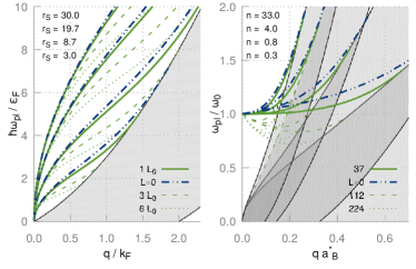
Figure 7: RPA plasmon with $\varphi_{{}_{0\!}}(z)$ of an infinite square well of width $L\!=\!0$ (dashed-dotted blue lines), $L_{0},\,3L_{0}$ and $6L_{0}$ (green full, dashed and dotted lines, respectively), corresponding to 370Å,  1120Å and 2240Å in AlGaAs. Left: $\omega_{\mathrm{pl}}(q)$ in Fermi units; the highest (lowest) group of curves are the highest (lowest) $r_{\scriptscriptstyle\mathrm{S}}$. Right: Ratio with the classical $\omega_{0}(q)\!\propto\!\sqrt{q}\,$; highest (lowest) group of curves: highest (lowest) density $n$ (in $10^{9}$cm^-2). Shaded: particle–hole band(s).

To get a quantitative estimate how large $q$ are influenced by the well width, Fig. 8 shows the critical $q_{c}^{L,0}$ for $L\!=\!0,\,L_{0},\,3L_{0}$ and $6L_{0}$. Note that, although $\omega^{L_{0},0\!}_{\mathrm{pl}}(q)$ is nearly identical with $\omega_{0}(q)$ for small and intermediate $q$, the difference in $q_{c}$ is substantial. This is a consequence of the tangential approach of the (G)RPA plasmon to the single–particle band. It demonstrates that for larger $q$ correlations are more important and differently affected by $L$ than for small ones.

Figure 8: Critical wave vector for Landau damping for the QWs of Fig. 7 (same line styles). The thin black line is where $\omega_{0}(q)$ hits the particle–hole band.

We conclude with an expression for the $L\!=\!0$ RPA critical wave vector,

$$q^{0,0}_{\mathrm{c}}\,a_{\scriptscriptstyle\mathrm{B}}^{*}\>\approx\>\frac{2\,\big{(}2^{1/6}\!-r_{\scriptscriptstyle\mathrm{S}}^{1/3}+2^{9/4}\,r_{\scriptscriptstyle\mathrm{S}}\big{)}}{r_{\scriptscriptstyle\mathrm{S}}^{1/3}\,\big{(}1+2^{5/2}\,r_{\scriptscriptstyle\mathrm{S}}\big{)}}\;,$$ (68)

which has an error of $\leq\!2\%$ except for very small $r_{\scriptscriptstyle\mathrm{S}}$.

References

- Wood [1933] R. Wood, Remarkable optical properties of the alkali metals, Physical Review 44 (1933) 353.
- Lang [1948] W. Lang, Geschwindigkeitsverluste mittelschneller Elektronen beim Durchgang durch dünne Metallfolien, Optik 3 (1948) 233–246.
- Ruthemann [1948] G. Ruthemann, Diskrete Energieverluste mittelschneller Elektronen beim Durchgang durch dünne Folien, Annalen der Physik 437 (1948) 113–134.
- Bohm and Pines [1953] D. Bohm, D. Pines, A collective description of electron interactions: III. Coulomb interactions in a degenerate electron gas, Physical Review 92 (1953) 609.
- Allen Jr et al. [1977] S. Allen Jr, D. Tsui, R. Logan, Observation of the two-dimensional plasmon in silicon inversion layers, Physical Review Letters 38 (1977) 980.
- Armbrust et al. [2016] N. Armbrust, J. Güdde, U. Höfer, S. Kossler, P. Feulner, Spectroscopy and Dynamics of a Two-Dimensional Electron Gas on Ultrathin Helium Films on Cu(111), Physical Review Letters 116 (2016) 256801.
- Sarma and Li [2013] S. D. Sarma, Q. Li, Intrinsic plasmons in two-dimensional Dirac materials, Physical Review B 87 (23) (2013) 235418.
- Ta Ho et al. [2014] S. Ta Ho, H. Anh Le, T. Le, D. Chien Nguyen, V. Nam Do, Effects of temperature, doping and anisotropy of energy surfaces on behaviors of plasmons in graphene, Physica E 58 (2014) 101–105.
- Van Tuan and Khanh [2013] D. Van Tuan, Q. N. Khanh, Plasmon modes of double-layer graphene at finite temperature, Physica E 54 (2013) 267–272.
- Hofmann and Das Sarma [2015] J. Hofmann, S. Das Sarma, Plasmon signature in Dirac-Weyl liquids, Physical Review B 91 (2015) 241108.
- Thakur et al. [2017] A. Thakur, R. Sachdeva, A. Agarwal, Dynamical polarizability, screening and plasmons in one, two and three dimensional massive Dirac systems, Journal of Physics: Condensed Matter 29 (2017) 105701.
- Grosu and Tugulan [2008] I. Grosu, L. Tugulan, Plasmon dispersion in quasi-one- and one-dimensional systems with non-magnetic impurities, Physica E 40 (3) (2008) 474–477.
- Giuliani and Vignale [2005] G. Giuliani, G. Vignale, Quantum theory of the electron liquid, Cambridge University Press, 2005.
- Lošić [2014] Ž. B. Lošić, Spectral function of the two-dimensional system of massless Dirac electrons, Physica E 58 (2014) 138–145.
- Vigil-Fowler et al. [2016] D. Vigil-Fowler, S. G. Louie, J. Lischner, Dispersion and line shape of plasmon satellites in one, two, and three dimensions, Physical Review B 93 (2016) 235446.
- Polini et al. [2008] M. Polini, R. Asgari, G. Borghi, Y. Barlas, T. Pereg-Barnea, A. H. MacDonald, Plasmons and the spectral function of graphene, Physical Review B 77 (2008) 081411.
- Nagao et al. [2001] T. Nagao, T. Hildebrandt, M. Henzler, S. Hasegawa, Dispersion and Damping of a Two-Dimensional Plasmon in a Metallic Surface-State Band, Physical Review Letters 86 (2001) 5747–5750.
- Rugeramigabo et al. [2008] E. P. Rugeramigabo, T. Nagao, H. Pfnür, Experimental investigation of two-dimensional plasmons in a DySi2 monolayer on Si(111), Phys. Rev. B 78 (2008) 155402.
- Hirjibehedin et al. [2002] C. F. Hirjibehedin, A. Pinczuk, B. S. Dennis, L. N. Pfeiffer, K. W. West, Evidence of electron correlations in plasmon dispersions of ultralow density two-dimensional electron systems, Physical Review B 65 (2002) 161309.
- Eriksson et al. [2000] M. Eriksson, A. Pinczuk, B. Dennis, C. Hirjibehedin, S. Simon, L. Pfeiffer, K. West, Collective excitations in low-density 2D electron systems, Physica E 6 (1) (2000) 165–168.
- Hao et al. [2015] X. Hao, Z. Wang, M. Schmid, U. Diebold, C. Franchini, Coexistence of trapped and free excess electrons in , Physical Review B 91 (2015) 085204.
- Faridi and Asgari [2017] A. Faridi, R. Asgari, Plasmons at the LaAlO3/SrTiO3 interface and in the graphene-LaAlO3/SrTiO3 double layer, Physical Review B 95 (2017) 165419.
- Böhm et al. [2010] H. M. Böhm, R. Holler, E. Krotscheck, M. Panholzer, Dynamic many-body theory: Dynamics of strongly correlated Fermi fluids, Physical Review B 82 (2010) 224505.
- Campbell et al. [2015] C. E. Campbell, E. Krotscheck, T. Lichtenegger, Dynamic many-body theory: Multiparticle fluctuations and the dynamic structure of , Physical Review B 91 (2015) 184510.
- Halinen et al. [2003] J. Halinen, V. Apaja, M. Saarela, Effect of external screening on plasmons, Physica E 18 (1) (2003) 346–347.
- Hwang and Das Sarma [2001] E. H. Hwang, S. Das Sarma, Plasmon dispersion in dilute two-dimensional electron systems: quantum–classical and Wigner crystal – electron liquid crossover, Physical Review B 64 (2001) 165409.
- Davoudi et al. [2001] B. Davoudi, M. Polini, G. F. Giuliani, M. P. Tosi, Analytical expressions for the charge-charge local-field factor and the exchange-correlation kernel of a two-dimensional electron gas, Physical Review B 64 (2001) 153101.
- Gori-Giorgi et al. [2004] P. Gori-Giorgi, S. Moroni, G. B. Bachelet, Pair-distribution functions of the two-dimensional electron gas, Physical Review B 70 (2004) 115102.
- Polini and Tosi [2006] M. Polini, M. Tosi, Many-body physics in condensed matter systems (Publications of the Scuola Normale Superiore) (v.4), Edizioni della Normale, ISBN 9788876421921, 2006.
- Moroni et al. [1992] S. Moroni, D. M. Ceperley, G. Senatore, Static response from quantum Monte Carlo calculations, Physical Review Letters 69 (1992) 1837–1840.
- Fabrocini et al. [2002] A. Fabrocini, S. Fantoni, E. Krotscheck, Introduction to Modern Methods of Quantum Many–Body Theory and their Applications, vol. 7 of Advances in Quantum Many–Body Theory, World Scientific, Singapore, 2002.
- Kreil et al. [2015] D. Kreil, R. Hobbiger, J. T. Drachta, H. M. Böhm, Excitations in a spin-polarized two-dimensional electron gas, Physical Review B 92 (2015) 205426.
- Senatore et al. [1996] G. Senatore, S. Moroni, D. M. Ceperly, The local field of the electron gas, in: W. D. W. D. Kraeft, M. Schlanges (Eds.), Proceedings of the (Binz Germany) International Conference on the Physics of Strongly Coupled Plasmas, World Scientific, Singapore, 429–434, 1996.
- Niklasson [1974] G. Niklasson, Dielectric function of the uniform electron gas for large frequencies or wave vectors, Physical Review B 10 (1974) 3052–3061.
- Bhukal et al. [2015] N. Bhukal, Priya, R. Moudgil, Dispersion of two-dimensional plasmons in GaAs quantum well and Ag monolayer, Physica E 69 (2015) 13–18.
- Aharonyan [2011] K. Aharonyan, Dielectric function and collective plasmon modes of a quasi-two-dimensional finite confining potential semiconductor quantum well, Physica E 43 (9) (2011) 1618–1624.
- Iwamoto [1984] N. Iwamoto, Sum rules and static local-field corrections of electron liquids in two and three dimensions, Physical Review A 30 (1984) 3289–3304.
- Mermin [1970] N. D. Mermin, Lindhard Dielectric Function in the Relaxation-Time Approximation, Physical Review B 1 (1970) 2362–2363.
- Holas and Rahman [1987] A. Holas, S. Rahman, Dynamic local-field factor of an electron liquid in the quantum versions of the Singwi-Tosi-Land-Sjölander and Vashishta-Singwi theories, Phys. Rev. B 35 (1987) 2720–2731.
- Yurtsever et al. [2003] A. Yurtsever, V. Moldoveanu, B. Tanatar, Dynamic correlation effects on the plasmon dispersion in a two-dimensional electron gas, Physical Review B 67 (2003) 115308.
- Tas and Tanatar [2010] M. Tas, B. Tanatar, Plasmonic contribution to the van der Waals energy in strongly interacting bilayers, Physical Review B 81 (2010) 115326.
- Neilson et al. [1991] D. Neilson, L. Świerkowski, A. Sjölander, J. Szymański, Dynamical theory for strongly correlated two-dimensional electron systems, Physical Review B 44 (1991) 6291–6305.
- Hobbiger et al. [2017] R. Hobbiger, J. T. Drachta, D. Kreil, H. M. Böhm, Phenomenological plasmon broadening and relation to the dispersion, Solid State Communications 252 (2017) 54 – 58.
- Sturm [1982] K. Sturm, Electron energy loss in simple metals and semiconductors, Advances in Physics 31 (1982) 1–64.
- Fukuda et al. [2007] T. Fukuda, N. Hiraiwa, T. Mitani, T. Toyoda, Plasmon dispersion of a two-dimensional electron system with finite layer width, Physical Review B 76 (2007) 033416.
- Godfrin et al. [2012] H. Godfrin, M. Meschke, H.-J. Lauter, A. Sultan, H. M. Böhm, E. Krotscheck, M. Panholzer, Observation of a roton collective mode in a two-dimensional Fermi liquid, Nature 483 (2012) 576–579.
- Agarwal et al. [2014] A. Agarwal, M. Polini, G. Vignale, M. E. Flatté, Long-lived spin plasmons in a spin-polarized two-dimensional electron gas, Physical Review B 90 (15) (2014) 155409.
- Asgari et al. [2005] R. Asgari, B. Davoudi, M. Polini, G. F. Giuliani, M. P. Tosi, G. Vignale, Quasiparticle self-energy and many-body effective mass enhancement in a two-dimensional electron liquid, Physical Review B 71 (2005) 045323.
- Asgari et al. [2009] R. Asgari, T. Gokmen, B. Tanatar, M. Padmanabhan, M. Shayegan, Effective mass suppression in a ferromagnetic two-dimensional electron liquid, Physical Review B 79 (2009) 235324.
- Krotscheck and Springer [2003] E. Krotscheck, J. Springer, Physical Mechanisms for Effective Mass Enhancement in 3He, Journal of Low Temperature Physics 132 (5) (2003) 281–295.
- Feenberg [1969] E. Feenberg, Theory of quantum fluids, Pure and applied physics, Academic Press, ISBN 9780122508509, 1969.
- Chang and Campbell [1976] C. C. Chang, C. E. Campbell, Density dependence of the roton spectrum in liquid , Physical Review B 13 (1976) 3779–3782.
- Wang et al. [2011] Y. Wang, E. W. Plummer, K. Kempa, Foundations of Plasmonics, Advances in Physics 60 (5) (2011) 799–898.