Fully Convolutional Measurement Network for Compressive Sensing Image Reconstruction

Abstract

Recently, deep learning methods have made a significant improvement in compressive sensing image reconstruction task. In the existing methods, the scene is measured block by block due to the high computational complexity. This results in block-effect of the recovered images. In this paper, we propose a fully convolutional measurement network, where the scene is measured as a whole. The proposed method powerfully removes the block-effect since the structure information of scene images is preserved. To make the measure more flexible, the measurement and the recovery parts are jointly trained. From the experiments, it is shown that the results by the proposed method outperforms those by the existing methods in PSNR, SSIM, and visual effect.

1 Introduction

Compressive sensing (CS) theory [1, 2, 3, 4] is able to acquire measurements of signals at sub-Nyquist rates and recover signals with high probability when the signals are sparse in a certain domain. Greedy algorithms [5, 6], convex optimization algorithms [7, 8], and iterative algorithms [9, 10] have been used for recovering images in conventional CS. However, almost all these methods recover images by solving an optimization problem, which is time-consuming. In order to reduce the computational complexity in the reconstruction stage, convolutional neural networks (CNNs) are applied to replace the optimization process. CNN-based methods [11, 12, 13, 14, 15] use big data [16] to train the networks that speed up the reconstruction stage. Mousavi, Patel, and Baraniuk [11] firstly propose deep learning approach to solve the CS recovery problem. They use stacked denoising autoencoders (SDA) to recover signals from undersampled measurements. ReconNet [12] and DeepInverse [13] introduce CNNs to the reconstruction problem, where the random Gaussian measurement matrix is used to generate the measurements. Instead, the methods [14, 15] using adaptive measurement learn a transformation from signals to the measurements. This mechanism allows measurements to retain more information from images. The methods mentioned above divide an image into blocks, which breaks the structure information of the image. This will cause the block effect in the reconstructed image.

In this paper, we propose a fully convolutional measurement network for CS image reconstruction. Instead of block-wise methods, a convolutional layer is applied to obtain the measurement from a full image, which keeps the integrity of structure information of the original image. Furthermore, motivated by the residual learning proposed by ResNet [17], we apply residual connection block (Resblock) in the proposed network for improvement. Experimental results show that the proposed method outperforms the state-of-the-art method 1$\sim$2dB in PSNR at different measurement rates.

The organization of this paper is as follows. The related works using deep learning methods for the CS reconstruction problem are introduced in Section 2. Section 3 presents the proposed fully convolutional measurement network. Section 4 shows experimental results of the proposed method and the previous works. The conclusion of this paper is drawn in Section 5.

2 Related Work

Recently, deep learning methods have been applied in CS image reconstruction tasks and achieve promising results such as [11, 12, 14]. Among them, CNN-based methods present superior performance. ReconNet [12] is a representative work that applies CNNs in reconstructing low-resolution mixed image measured by random Gaussian matrix. The framework is shown in Fig. 1.

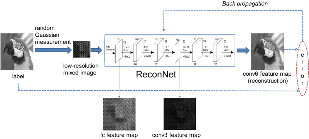
Figure 1: Framework of random Gaussian based network.

The training of the network is driven by the error between the label and the reconstructed image. And the loss function is given by

$$L(\{W\})=\frac{1}{T}\sum_{i=1}^{T}{\lVert f(y_{i},\{W\})-x_{i}\rVert}^{2},$$ (1)

where $f(y_{i},\{W\})$ is the $i-th$ reconstructed image of ReconNet. $x_{i}$ is the $i-th$ original signal as well as the $i-th$ label. $\{W\}$ means the training parameters in ReconNet. $T$ is the total number of image blocks in the training dataset. The loss function is minimized by tuning $\{W\}$ using back propagation.

Based on the way the original image is measured, deep learning methods for CS reconstruction can be divided into two categories: fixed random Gaussian measurement and adaptive measurement.

Fixed random Gaussian measurement

Mousavi et al. [11] firstly use SDA to recover signals from undersampled measurements. ReconNet [12] and DeepInverse [13] utilizes CNNs to recover signals from Gaussian measurements. DR²-Net [18], inheriting ReconNet, adds residual connection blocks (Resblock) to its reconstruction stage and achieves better performance. Instead of learning to directly reconstruct the high-resolution image from the low-resolution one, DR²-Net learns the residual between the ground truth image and the preliminary reconstructed image. However, the measurements of these methods are randomly measured, which is not optimally designed for natural images.

Adaptive measurement

In order to keep the information of the training data, the adaptive measurement is proposed. Methods including improved ReconNet [19], Adp-Rec [15], and DeepCodec [14] are all based on adaptive measurement. In cases of the improved ReconNet and Adp-Rec, a fully-connected layer is used to measure the signals, which allows for a jointly learning of the measurement and reconstruction stages. With the learned measurement matrix, a significant gain in terms of PSNR is achieved. DeepCodec, closely related to the DeepInverse, learns a transformation for dimensionality reduction. Learning measurements from the original signals helps to preserve more information compared with taking random measurements.

3 Fully Convolutional Measurement

The exsiting CNN-based CS methods always adopt block-wise pattern due to the limitation of GPU memory. The block effect comes accordingly. In order to overcome this shortcoming, we propose a fully convolutional measurement network in which a convolutional layer is used to get the adaptive measurements. It is different from our previous work using fully-connected layers [15]. Fig. 2 shows the proposed network which is composed of a convolutional layer, a deconvolutional layer [20], and a residual block. The first layer ‘conv’ is used to obtain measurements. The second layer ‘deconv’ is used to recover a low resolution image from the measurements. Furthermore, we apply a residual network (ResNet) to reconstruct the high resolution image. Because batch normalization would get rid of range flexibility from networks [21], we remove the batch normalization layer in Resblock. Our framework is different from super-resolution (SR) [22] [23] [24] [25], since SR just learns a transform form the low-resolution images to high-resolution images, while the proposed framework is jointly trained from the measurement to the recovery part.

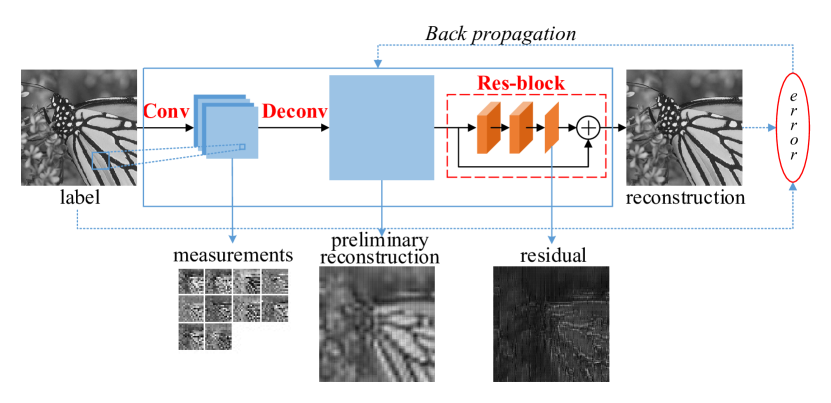
Figure 2: Framework of the proposed network.

The loss function of the proposed network is given by

$$L(\{W\})=\frac{1}{T}\sum_{i=1}^{T}{\lVert f(x_{i},\{W,K\})-x_{i}\rVert}^{2},$$ (2)

where $K$ is the parameter of the convolutional measurement network, and $W$ is the parameters of the reconstruction network. The Euclidian distance between the label and the reconstruction is back propagated to train the whole network.

The main advantage of the proposed network is the use of convolutional layer as the measurement matrix. By means of the overlapped convolutional kernels, this structure can remove block effect of the reconstructed images. In details, one feature map contains several measurements of each pixel, which is similar to the idea proposed by He et al. [26] that the feature map preserves the explicit per-pixel spatial correspondence. Another advantage is that the fully convolutional neural network can deal with images of any size, which breaks the limitation that fully-connected layer is only capable of measuring the fixed size of images. Once the network is trained, we can test images with different sizes without changing the structure of the network.

Fig. 3 shows an example of reconstruction results at three kinds of measurements. The original image and those by random Gaussian, Adp-Rec, and the proposed method are shown respectively in Fig. 3(a), (b), (c), and (d). The measurement rate is 10%. We can see that the proposed method performs better than the others.

(a) Origin

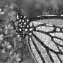
(b) ReconNet
(21.49dB)

(c)  Adp-Rec
 (26.65dB)

(d) Proposed
(27.61dB)

Figure 3: The reconstruction results of monarch at measurement rate 10%.

The better performance can be proved through a visualization of the kernels in convolutional layer of the measurement network, as shown in Fig. 4. Since the original signal in random Gaussian and adaptive measurements is a cloumn vector (Fig. 4(a) and (b)), we reshape the row vectors of measurement matrix to size $33\times 33$. Fig. 4(a) shows two reshaped row vectors of the random Gaussian measurement matrix at measurement rates 1% , 10%, and 25% in both time and frequency domain. The content of random Gaussian measurement matrix is obviously irregular. Fig. 4(b) shows two reshaped row vectors of adaptive measurement matrix in Adp-Rec. When measurement rate is set to 1%, low frequency information is already extracted. As the measurement rate increases, much high frequency information is captured. Fig. 4(c) shows two kernels of the proposed measurement matrix. Compared with the adaptive measurements in Adp-Rec, the measurements by the proposed method provide more concentrated energy in the low frequency area at different measurement rates. As for the directional information, when measurement rate is 1%, two extracted typical directions ‘horizontal’ and ‘vertical’ can be easily observed in time domain.

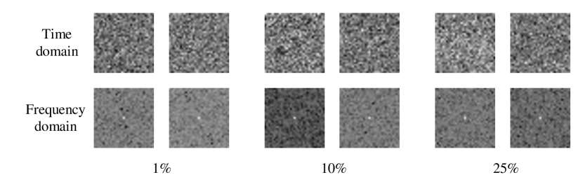
(a) Random Gaussian measurements.

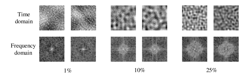
(b) Adaptive measurements in Adp-Rec.

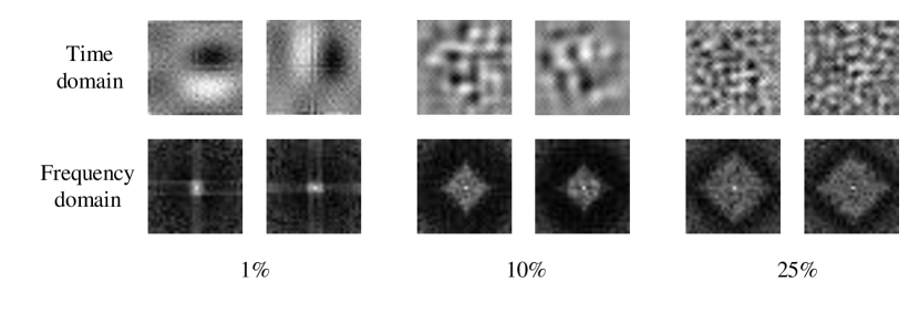
(c) Proposed

Figure 4: Reshaped row vectors of measurement matrix at measurement rates 1%, 10%, and 25% in both time and frequency domain.

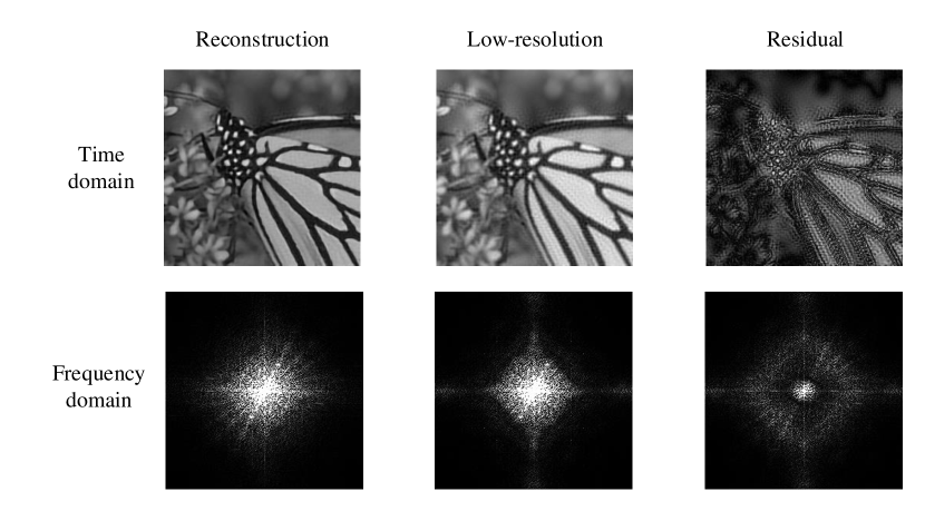
Figure 5: Reconstruction image, low-resolution image and residual image at measurement rate 10% in both time and frequency domain.

Fig. 5 shows the reconstruction of image ‘Monarch’, its low-resolution, and the corresponding residual. From residual image in frequency domain, we can see that the high frequency component is mainly learned by the residual network. Rather than ReconNet which reconstructs the high resolution image from the low resolution one directly, ResNet just reconstruct the residual between the low resolution image and the high resolution image, that is the reconstruction image. Thus, all its energy is concentrated on the residual. That is why ResNet has better performance.

4 Experiments

In this section, we perform experiments on the reconstruction of compressive sensing images with existing typical methods. The results show the outstanding performance by the proposed method.

The experiments are conducted on caffe framework [27]. Our computer is equipped with Intel Core i7-6700 CPU with frequency of 3.4GHz, 4 NVidia GeForce GTX Titan XP GPUs, 128 GB RAM, and the framework runs on Ubuntu 16.04 operating system. The training dataset consists of 800 pieces of $256\times 256$ size images downsampled and divided from 800 images in DIV2K dataset [28].

The performance of the proposed method is compared with those by ReconNet and Adp-Rec which are the typical CNN-based CS methods. We give the testing results using image ‘parrots’, ‘flinstones’, and ‘cameraman’ at measurement rates 1%, 10%, and 25%, as shown in Fig. 6, Fig. 7, and Fig. 8, respectively. The proposed method provides the best reconstruction results in terms of PSNR and the results are most visually attractive.

From the results shown in Fig. 6, with measurement rate being 1%, it can be seen that the block effect is removed (Fig 6(d) vs. (b) and (c)). From Fig. 7, when the measurement rate is 10%, the proposed method shows the advantage in reconstructing the image, typically in those smooth areas such as nose, hands, and legs of the man. From Fig. 8, when measurement rate rises to 25%, the proposed method still outperforms other methods, which can be easily seen in the edge of the man’s arm.

(a) Origin

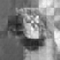
(b) ReconNet
(18.93dB)

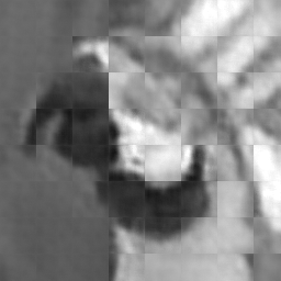
(c)  Adp-Rec
 (21.67dB)

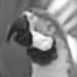
(d) Proposed
(22.49dB)

Figure 6: The reconstruction results of parrots at measurement rate 1%.

(a) Origin

(b) ReconNet
(19.04dB)

(c)  Adp-Rec
 (23.83dB)

(d) Proposed
(24.98dB)

Figure 7: The reconstruction results of flinstones at measurement rate 10%.

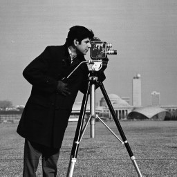
(a) Origin

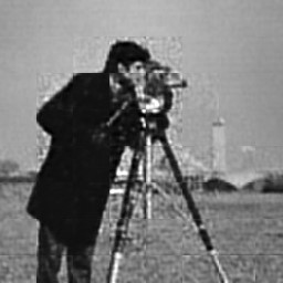
(b) ReconNet
(23.48dB)

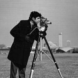
(c)  Adp-Rec
 (27.11dB)

(d) Proposed
(28.99dB)

Figure 8: The reconstruction results of cameraman at measurement rate 25%.

For an overall look on the performance, the reconstruction results of 11 test images at measurement rates 1%, 10%, and 25% with the methods including ReconNet, DR²-Net, Adp-Rec, Fully-Conv, and the proposed one are shown in Table 1. The mean PSNR is given in the type of blue background. It is obvious that the proposed method shows greatest performance in almost all test images.

Table 1: The PSNR results at measurement rates (MR) 1%, 10%, and 25%, where Red is ranked the first and blue is ranked the second.

MR	Samples	ReconNet	$\bf{DR^{2}}$-Net	Adp-Rec	Fully-Conv	Proposed
1%	Monarch	15.61dB	15.33dB	17.70dB	17.98dB	18.46dB
	Parrots	18.93dB	18.01dB	21.67dB	21.80dB	22.49dB
	Barbara	19.08dB	18.65dB	21.36dB	21.61dB	22.06dB
	Boats	18.82dB	18.67dB	21.09dB	21.73dB	22.3dB
	Cameraman	17.51dB	17.08dB	19.74dB	19.88dB	20.63dB
	Fingerprint	15.01dB	14.73dB	16.22dB	16.24dB	16.33dB
	Flinstones	14.14dB	14.01dB	16.12dB	16.55dB	16.92dB
	Foreman	22.03dB	20.59dB	25.53dB	25.18dB	27.26dB
	House	20.30dB	19.61dB	22.93dB	22.93dB	23.67dB
	Lena	18.51dB	17.97dB	21.49dB	21.77dB	22.51dB
	Peppers	17.39dB	16.90dB	19.75dB	20.80dB	21.38dB
	Mean(all)	17.94dB	17.44dB	20.33dB	20.59dB	21.27dB
10%	Monarch	21.49dB	23.10dB	26.65dB	25.20dB	27.61dB
	Parrots	23.36dB	23.94dB	27.59dB	26.82dB	27.92dB
	Barbara	22.17dB	22.69dB	24.28dB	24.39dB	24.28dB
	Boats	24.56dB	25.58dB	28.80dB	28.52dB	29.48dB
	Cameraman	21.54dB	22.46dB	24.97dB	24.58dB	25.62dB
	Fingerprint	20.99dB	22.03dB	26.55dB	26.92dB	27.36dB
	Flinstones	19.04dB	21.09dB	23.83dB	23.08dB	24.98dB
	Foreman	29.02dB	29.20dB	33.51dB	31.96dB	34.00dB
	House	26.74dB	27.53dB	31.43dB	30.81dB	32.36dB
	Lena	24.48dB	25.39dB	28.50dB	27.76dB	28.97dB
	Peppers	22.72dB	24.32dB	26.67dB	26.69dB	28.72dB
	Mean(all)	23.28dB	24.32dB	27.53dB	26.98dB	28.30dB
25%	Monarch	24.95dB	27.95dB	29.25dB	28.47dB	32.63dB
	Parrots	26.66dB	28.73dB	30.51dB	29.90dB	32.13dB
	Barbara	23.58dB	25.77dB	27.40dB	27.11dB	28.59dB
	Boats	27.83dB	30.09dB	32.47dB	31.75dB	33.88dB
	Cameraman	23.48dB	25.62dB	27.11dB	26.73dB	28.99dB
	Fingerprint	26.15dB	27.65dB	32.31dB	30.92dB	32.91dB
	Flinstones	22.74dB	26.19dB	27.94dB	27.02dB	30.26dB
	Foreman	32.08dB	33.53dB	36.18dB	35.08dB	38.10dB
	House	29.96dB	31.83dB	34.38dB	33.63dB	36.22dB
	Lena	27.47dB	29.42dB	31.63dB	30.65dB	33.00dB
	Peppers	25.74dB	28.49dB	29.65dB	29.71dB	32.90dB
	Mean(all)	26.42dB	28.66dB	30.80dB	30.09dB	32.69dB

Table 2: The SSIM and MOS results. Here measurement rates (MR) 1% is taken as an example. The highest is marked red, while the second is marked blue.

	Samples	Original	ReconNet	$\bf{DR^{2}}$-Net	Adp-Rec	Proposed
MOS	Monarch	4.9615	1.0000	1.1538	1.7307	2.4615
	Parrots	4.9615	1.0384	1.2307	2.1538	2.9230
	Barbara	4.9615	1.0769	1.0769	2.0000	2.6538
	Boats	4.9230	1.0769	1.0384	1.5000	2.3846
	Cameraman	5.0000	1.1538	1.1923	1.8461	2.7692
	Fingerprint	4.8461	1.1538	1.0384	1.4230	1.6823
	Flinstones	5.0000	1.1923	1.1538	2.0769	3.1538
	Foreman	4.9230	1.1538	1.1538	1.9230	2.7692
	House	4.9615	1.0000	1.1153	2.0769	2.7307
	Lena	5.0000	1.0384	1.0384	1.8076	2.8461
	Peppers	4.9615	1.0000	1.1153	1.8076	2.5769
	Mean(all)	4.9545	1.0734	1.1188	1.8496	2.6328
SSIM	Monarch	1.0000	0.3801	0.3931	0.4755	0.5058
	Parrots	1.0000	0.5328	0.5617	0.6739	0.7135
	Barbara	1.0000	0.3729	0.3847	0.4648	0.5007
	Boats	1.0000	0.4140	0.4319	0.4888	0.5405
	Cameraman	1.0000	0.4516	0.4783	0.5578	0.5867
	Fingerprint	1.0000	0.1548	0.1727	0.1628	0.1700
	Flinstones	1.0000	0.2502	0.2718	0.3230	0.3801
	Foreman	1.0000	0.5647	0.6051	0.6912	0.7396
	House	1.0000	0.5278	0.5526	0.6350	0.6624
	Lena	1.0000	0.4418	0.4552	0.5554	0.6081
	Peppers	1.0000	0.4002	0.4127	0.5053	0.5839
	Mean(all)	1.0000	0.4083	0.4291	0.5031	0.5447

From Table 1, it can be concluded that Adp-Rec beats DR²-Net and ReconNet about 3dB in all measurement rates because of its adaptive measurement. Based on the standard ReconNet [12], the improved ReconNet [19] adds several tricks such as adaptive measurement and adversarial loss. Its performance is even lower than Adp-Rec. Despite its promising results, Adp-Rec still divides image into blocks, ignoring the relevance between neighbouring blocks, which causes to the block effect in reconstructed images. For this reason, Fully-Conv uses a convolution layer as measurement matrix to deal with this problem. It achieves comparable results with Adp-Rec even though it contains no additional operation.

To further improve the reconstruction results, we put Resblock after Fully-Conv structure because of the brilliant performance of Resblock in reconstruction task. With this enhancement, the proposed method obtains the best performance in terms of PSNR at all measurement rates, as shown in Table 1.

We also measure the quality of images with Mean Opinion Score (MOS). The test results of different images are shown in Table 2. In this experiment, 26 volunteers take part in ranking the images. The quality of the images is divided into five levels, from 1 to 5, with the quality from low to high. All the test images are randomly ranked before being scored and they are displayed group by group. Each group has four reconstruction images, in different methods, and one original scene image. All participants take this test on the same computer screen, from the same angle and distance. Here the distance from the screen to the tested persons is 50 cm and the eyes of those persons are of the same height of the center of the screen. In addition, we also use structural similarity index (SSIM) to evaluate our method and existing block-wised methods as shown in Table 2. The case of MR = 1% is taken as an example.

In terms of hardware implementation, we follow the approach of the previous work proposed in [29] in which sliding window is used to measure the scene. Similarly, we can replace the random Gaussian measurement matrix with the learned pre-defined parameters in the conv layer of the measurement network. The reconstruction part is not on optical device, so only the measurement part needs to be implemented with the approach above.

5 Conclusion

This paper proposes a novel CNN-based deep neural network for high-quality compressive sensing image reconstruction. The network uses a fully convolutional architecture, which removes the block effect caused by block-wise methods. For a further improvement, we add Resblock after the deconvolutional layer, making the network learn the residual information between low and high resolution images. With this enhancement, the network shows best performance in reconstruction task compared with other methods. In future work, we are going to apply perceptual loss into the network for better reconstruction result. And semantics-oriented reconstruction will be also considered.

References

- [1] R. G. Baraniuk, V. Cevher, M. F. Duarte, C. Hegde, Model-based compressive sensing, IEEE Trans. Inform. Theory 56 (4) (2010) 1982–2001.
- [2] R. G. Baraniuk, More is less: Signal processing and the data deluge, Science 331 (6018) (2011) 717–719.
- [3] E. Candes, J. Romberg, Sparsity and incoherence in compressive sampling, Inverse Probl. 23 (3) (2007) 969.
- [4] J. Haupt, W. U. Bajwa, G. Raz, R. Nowak, Toeplitz compressed sensing matrices with applications to sparse channel estimation, IEEE Trans. Inform. Theory 56 (11) (2010) 5862–5875.
- [5] D. Needell, J. A. Tropp, Cosamp: iterative signal recovery from incomplete and inaccurate samples, Commun. ACM 53 (12) (2010) 93–100.
- [6] S. D. Babacan, R. Molina, A. K. Katsaggelos, Bayesian compressive sensing using laplace priors, IEEE Trans. Image Processing 19 (1) (2010) 53–63.
- [7] E. J. Candes, T. Tao, Decoding by linear programming, IEEE Trans. Inform. Theory 51 (12) (2005) 4203–4215.
- [8] M. A. Figueiredo, R. D. Nowak, S. J. Wright, Gradient projection for sparse reconstruction: Application to compressed sensing and other inverse problems, IEEE J. Sel. Top. Sign. Proces. 1 (4) (2007) 586–597.
- [9] D. L. Donoho, A. Maleki, A. Montanari, Message-passing algorithms for compressed sensing, P. Natl. A. Sci. 106 (45) (2009) 18914–18919.
- [10] I. Daubechies, M. Defrise, C. De Mol, An iterative thresholding algorithm for linear inverse problems with a sparsity constraint, Commun. Pur. Appl. Math. 57 (11) (2004) 1413–1457.
- [11] A. Mousavi, A. B. Patel, R. G. Baraniuk, A deep learning approach to structured signal recovery, in: Annual Allerton Conference on Communication, Control, and Computing, IEEE, 2015, pp. 1336–1343.
- [12] K. Kulkarni, S. Lohit, P. Turaga, R. Kerviche, A. Ashok, Reconnet: Non-iterative reconstruction of images from compressively sensed measurements, in: Proceedings of the IEEE Conference on Computer Vision and Pattern Recognition, 2016, pp. 449–458.
- [13] A. Mousavi, R. G. Baraniuk, Learning to invert: Signal recovery via deep convolutional networks, in: Proceedings of the IEEE International Conference on Acoustics, Speech and Signal Processing, 2017.
- [14] A. Mousavi, G. Dasarathy, R. G. Baraniuk, Deepcodec: Adaptive sensing and recovery via deep convolutional neural networks, in: arXiv preprint arXiv:1707.03386, 2017.
- [15] X. Xie, Y. Wang, G. Shi, C. Wang, J. Du, X. Han, Adaptive measurement network for cs image reconstruction, in: China Conference on Computer Vision, 2017.
- [16] A. Stevens, N. D. Browning, Less is more: Bigger data from compressive measurements, Microscopy and Microanalysis 23 (S1) (2017) 166–167.
- [17] K. He, X. Zhang, S. Ren, J. Sun, Deep residual learning for image recognition, in: Proceedings of the IEEE conference on computer vision and pattern recognition, 2016, pp. 770–778.
- [18] H. Yao, F. Dai, D. Zhang, Y. Ma, S. Zhang, Y. Zhang, DR2-net: Deep residual reconstruction network for image compressive sensing, in: arXiv preprint arXiv:1702.05743, 2017.
- [19] S. Lohit, K. Kulkarni, R. Kerviche, P. Turaga, A. Ashok, Convolutional neural networks for non-iterative reconstruction of compressively sensed images, in: arXiv preprint arXiv:1708.04669, 2017.
- [20] L. Xu, J. S. Ren, C. Liu, J. Jia, Deep convolutional neural network for image deconvolution, in: Advances in Neural Information Processing Systems, 2014, pp. 1790–1798.
- [21] B. Lim, S. Son, H. Kim, S. Nah, K. M. Lee, Enhanced deep residual networks for single image super-resolution, in: IEEE Conference on Computer Vision and Pattern Recognition Workshops, 2017.
- [22] C. Deng, J. Xu, K. Zhang, D. Tao, X. Gao, X. Li, Similarity constraints-based structured output regression machine: An approach to image super-resolution, IEEE transactions on neural networks and learning systems 27 (12) (2016) 2472–2485.
- [23] X. Fan, Y. Yang, C. Deng, J. Xu, X. Gao, Compressed multi-scale feature fusion network for single image super-resolution, Signal Processing.
- [24] C. Dong, C. C. Loy, K. He, X. Tang, Image super-resolution using deep convolutional networks, IEEE transactions on pattern analysis and machine intelligence 38 (2) (2016) 295–307.
- [25] C. Ledig, L. Theis, F. Huszar, J. Caballero, A. Cunningham, A. Acosta, A. Aitken, A. Tejani, J. Totz, Z. Wang, W. Shi, Photo-realistic single image super-resolution using a generative adversarial network, in: The IEEE Conference on Computer Vision and Pattern Recognition (CVPR), 2017.
- [26] K. He, G. Gkioxari, P. Dollár, R. Girshick, Mask r-cnn, in: IEEE International Conference on Computer Vision, 2017.
- [27] Y. Jia, E. Shelhamer, J. Donahue, S. Karayev, J. Long, R. Girshick, S. Guadarrama, T. Darrell, Caffe: Convolutional architecture for fast feature embedding, in: Proceedings of the 22nd ACM international conference on Multimedia, 2014, pp. 675–678.
- [28] R. Timofte, E. Agustsson, L. Van Gool, M.-H. Yang, L. Zhang, B. Lim, S. Son, H. Kim, S. Nah, K. M. Lee, et al., Ntire 2017 challenge on single image super-resolution: Methods and results, in: IEEE Conference on Computer Vision and Pattern Recognition Workshops, 2017, pp. 1110–1121.
- [29] G. Shi, D. Gao, X. Song, X. Xie, X. Chen, D. Liu, High-resolution imaging via moving random exposure and its simulation, IEEE Transactions on Image Processing 20 (1) (2011) 276–282.