Bubble propagation on a rail: a concept for sorting bubbles by size^†

Andrés Franco-Gómez^a, Alice B. Thompson^b, Andrew L. Hazel^b, and Anne Juel^∗a

Received Xth XXXXXXXXXX 20XX, Accepted Xth XXXXXXXXX 20XX
First published on the web Xth XXXXXXXXXX 200X

DOI: 10.1039/b000000x

We demonstrate experimentally that the introduction of a rail, a small height constriction, within the cross-section of a rectangular channel could be used as a robust passive sorting device in two-phase fluid flows. Single air bubbles carried within silicone oil are generally transported on one side of the rail. However, for flow rates marginally larger than a critical value, a narrow band of bubble sizes can propagate (stably) over the rail, while bubbles of other sizes segregate to the side of the rail. The width of this band of bubble sizes increases with flow rate and the size of the most stable bubble can be tuned by varying the rail width. We present a complementary theoretical analysis based on a depth-averaged theory, which is in qualitative agreement with the experiments. The theoretical study reveals that the mechanism relies on a non-trivial interaction between capillary and viscous forces that is fully dynamic, rather than being a simple modification of capillary static solutions.

1 Introduction

The development of methods for sorting bubbles, droplets or particles within a suspending fluid is of fundamental importance to applications in biology, chemistry and industry. Consequently, a vast array of techniques for the active sorting of suspended components in microfluidic devices have been developed¹, often with particular applications in flow cytometry². Active sorting methods rely on inducing local motion of the suspended components via external forcing, e. g. electrical, magnetic and acoustic forces or external pressure; and typically require additional detection methods to ensure that the external forcing is actuated at the appropriate point in time. In contrast, passive approaches rely on harnessing the local motions of the suspended objects that arise through pure hydrodynamic interactions between the flow, the suspended object itself and the bounding geometry³; hence, the presence of the particles does not need to be detected. Thus passive sorting methods are simpler, and potentially more robust and energy efficient than their active counterparts.

For flows within channels and tubes, hydrodynamic interactions can lead to migration of particles, bubbles and droplets normal to the predominant direction of flow and their accumulation at particular locations within the channel cross-section⁴. Once such spatial localisation has been achieved, it is straightforward to use geometric separators to collect the suspended objects with the desired properties. Applications of passive methods include segregation of blood components⁵, trapping of micro-organisms in water⁶, and purification of emulsions or colloids.

The small scale of microfluidic devices means that inertial migration mechanisms^{7, 8} do not necessarily operate effectively, although recent work has shown that inertial microfluidics is feasible⁹. In this paper we shall concentrate on hydrodynamic mechanisms that operate on suspended gas bubbles and rely on an interplay between surface tension and viscous forces. The relative importance of viscous forces compared to surface tension can be quantified by a non-dimensional flow rate, $Q=\mu^{*}U^{*}_{0}/\sigma^{*}$, where $\mu^{*}$ is the viscosity of the suspending fluid, $U^{*}_{0}$ is the average flow velocity and $\sigma^{*}$ is the surface tension at the interface between the suspending fluid and gas bubble. In the absence of fluid inertia, rigid spherical particles do not migrate normal to the direction of flow⁷ and hence, as highlighted by many authors, the deformation of droplets or bubbles is an essential part of their underlying migration mechanism in slow flows^{3, 4}. For pressure-driven flow, in geometrically symmetric channels a deformable object will migrate away from the walls towards the centre of the channel¹⁰. Hence, the development of passive sorting techniques that can take advantage of the interaction between surface tension and viscous forces requires a means to induce new geometrically distinct, off-centre, propagation modes where bubbles or droplets displace steadily near the channel walls and parallel to the fluid flow.

One method for passively controlling bubble or droplet location in the absence of inertia is to induce geometric variation within the channel cross-section. The introduction of grooves and holes into the top surface of a microchannel allows droplets or vesicles to reduce their surface energy by expanding into the available space^{11, 12}. Thus, by placing these grooves off-centre, droplets are anchored to the groove and can be guided to desired locations under moderate flow rates¹¹. Furthermore, multiple grooves of different widths can be used to sort droplets by their size or capillary number¹³. The fundamental anchoring mechanism is based on modification of the capillary-static solution, a mechanism that operates for bubbles at both millimetric and micrometric scales¹⁴. If the bubble is forced instead to contract via the introduction of a localised obstacle, capillary forces will drive the bubble away from the constricted region. This effect has recently been used to facilitate faster fluorescence-activated sorting by Sciambi & Abate¹⁵, who used what they termed a “gapped divider” that occluded approximately one third of the channel’s height.

In this work, we study the propagation of finite air bubbles using silicone oil as a carrier fluid in a channel with a rectangular cross-section of high aspect ratio (width of the channel over its height $\alpha\gg 1$) in which a small centred height constriction that we term a “rail” is introduced in the longitudinal direction of the channel. We restrict attention to bubbles with diameters (when viewed from above) between 70% and 180% of the width of the rail. Our selected channel geometry is sometimes known as a Hele-Shaw cell, where in the absence of height variation, only centred bubbles will propagate stably for non-zero values of the surface tension¹⁶. In this geometry, static bubbles that do not span the full channel width are neutrally stable and can be located anywhere within the cross-section provided that they do not interact with the sidewalls. Thus, there must be a dynamic (flow-induced) restoring mechanism which ensures that off-centre bubbles return to the centreline of the channel. The restoring mechanism involves an interplay between the viscous pressure gradient, droplet shape and capillary pressure drop over the interface and does not appear to have been comprehensively elucidated in the Hele-Shaw-cell literature, although it is fundamentally the same as mechanisms operating in two-dimensional¹⁷ and three-dimensional¹⁸ Stokes flows. As described above, the introduction of a central rail leads to modification of the capillary-static solutions such that bubbles are driven away from the centre of the channel for low to moderate flow rates¹⁵. However, higher flow rates offer the possibility of dynamic stabilisation of the central “on-rail” propagation mode through a similar interaction between viscous and surface tension forces to that in the unoccluded Hele-Shaw cell. The stabilisation of the “on-rail” propagation mode at high flow rates is the principal focus of this paper.

In fact, our experimental results reveal that stable propagation over the rail is only possible for a limited range of bubble sizes. We find that the critical flow-rate for stable propagation depends non-monotonically on bubble size and that for a fixed flow rate marginally larger than the minimum critical flow rate, only a narrow range of bubble sizes will propagate stably over the rail. Numerical computations using a depth-averaged model reveal that this feature arises through the evolving location of a symmetry-breaking bifurcation as a function of bubble size and, moreover, that the dynamic stabilisation of these intermediate-sized bubbles arises through a non-trivial interaction between both viscous and surface-tension forces. In contrast, bubbles of all sizes considered can always propagate stably in an off-centred position. Thus, the introduction of the rail can be used to design a passive bubble sorting device that selects a restricted range of bubble sizes, as sketched in figure 1.

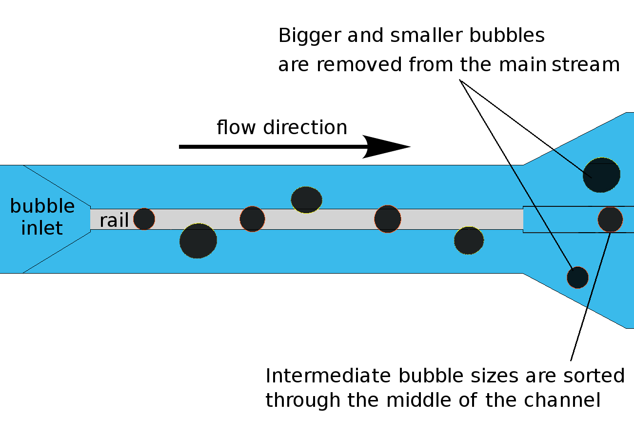
Fig.  1: In a channel of rectangular cross section bubbles typically propagate along the centreline. Upon the introduction of a centred rail within such a channel, we find that near a critical flow rate only a limited range of bubble sizes can propagate along the centreline, which provides a passive (geometric) mechanism for sorting bubbles by size. The critical flow rate and range of selected bubble sizes are set by the rail width.

In sections 2 and 3 we describe our experimental setup and numerical model, respectively. In section 4, we describe our results starting with the experimental evidence supporting passive bubble sorting. This is followed by a comparison with the results of our depth-averaged model, which in turn provides an explanation of the mechanisms underlying the process. Finally, we draw our conclusions in section 5.

2 Experimental methods

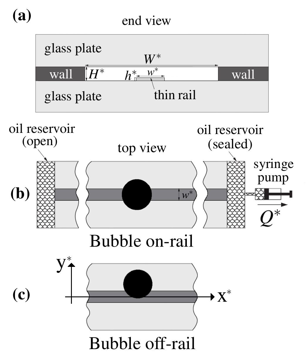
Fig.  2: Schematic diagram of the experimental system. (a) Cross-sectional view of the channel with a prescribed depth variation: an axially uniform, thin rail is positioned on the bottom boundary, symmetrically about the centreline of the channel. (b) Top view of the experimental system. An air bubble is propagated in an on-rail position by withdrawing liquid with constant volume-flux from one end of the channel using a syringe pump. (c) Schematic diagram of a bubble propagating in an off-rail position, indicating the Cartesian coordinate system used.

A schematic diagram of the experimental setup is shown in figure 2. Note that all dimensional variables are starred. The flow channel was made of two parallel glass plates of dimensions $60$ cm $\times$ $10$ cm $\times$ $2$ cm separated by brass sheets of uniform height $H^{*}=1$ mm, so that the depth of the channel was accurate to within $0.1\%$. The width of the channel was set to $W^{*}=30\pm 0.1$ mm, and thus the aspect ratio was $\alpha=W^{*}/H^{*}=30$. A prescribed depth profile was introduced by bonding a rectangular strip of polypropylene film of thickness $h^{*}=24\pm 1$ $\mu$m (i.e. $2.4$ % of the total height of the channel) along the centreline of the bottom boundary, which hereinafter will be referred to as the rail (figure 2a). Two different rail widths were used: $w^{*}=6.9\pm 0.1$ mm and $10.7\pm 0.1$ mm. The positional accuracy of the rail was such that the widths of the full-height channels on both sides of the rail differed by less than $1$ % ($<100$ $\mu$m) over the entire length of the channel. The channel was levelled horizontally to within $\pm 0.05^{\circ}$.

A syringe pump (KDS210) was used to fill the channel with silicone oil (Basildon Chemicals Ltd.) of viscosity $\mu^{*}=5\times 10^{-2}$ Pa s, density $\rho^{*}=961$ kg m^-3 and surface tension $\sigma^{*}=2.1\times 10^{-2}$ N m^-1 at the laboratory temperature of $21^{\circ}$C, via the sealed reservoir at one end of the channel (figure 2b). At the other end of the channel, oil was allowed to accumulate in an open reservoir. A single bubble was introduced in the channel with a $5$ ml glass syringe (Hamilton Gastight) connected to a $10$ cm long needle with a diameter of $0.8$ mm, inserted into the open end of the channel. The bubble was then propagated by withdrawing oil using the syringe pump at a constant value of the flow rate $Q^{*}$ in the range $1\leq Q^{*}\leq 50$ ml/min. Once the bubble had travelled the length of the channel, it was returned to the inlet by infusing oil back into the channel. At the start of each experiment, the bubble was approximately at rest and positioned either centrally in the channel (on-rail, figure 2b), or asymmetrically about the centreline of the channel (off-rail, figure 2c). For the range of bubble sizes investigated, the on-rail initial position was unstable, and thus it could only be imposed transiently (see Supplementary Material for details).

The propagation of bubbles was recorded with a DALSA Genie TS-M3500 camera with a $35$ mm f/1.4 lens (Carl Zeiss T^∗ Distagon) mounted at a distance of $0.94$ m above the experiment. The channel was back-lit with white light of uniform intensity provided by a custom-made LED light box aligned under the channel. The field of view of the camera was a channel section of dimensions $262.0$ mm $\times$ $30.0$ mm, and the image resolution of $1920\times 220$ pixels yielded $136.4$ $\mu$m/px. Depending on the value of $Q^{*}$, time-sequences of $400\geq N\geq 120$ images were recorded at frame rates $1\leq f^{*}\leq 10$ frames per second. An image processing algorithm developed in Matlab (MATLAB R2014a) was used to extract the outline of the propagating bubbles ¹⁹ as a function of time. The edge of the bubble coincides with the external edge of the outline, determined to within $0.14$ mm. The projected area $A^{*}$ of the bubble was calculated from the extracted outline. The centroid of this projected area was then determined to yield its displacement from the centreline of the channel, $y_{c}^{*}$. The size of the bubble was characterised by its diameter $D^{*}=2\sqrt{A^{*}/\pi}$ at rest off the rail. The range of diameters investigated was between $18\%$ and $49\%$ of the channel width. Given that the depth of the channel was $1/30$ of its width, this meant that the bubbles were strongly confined into a quasi-two-dimensional shape with thin liquid films separating the bubble interface from the top and bottom boundaries of the channel. Hereafter, we will quote diameters relative to the width of the rail, $D=D^{*}/w^{*}$. The evolution of the dimensionless centroid position $y_{c}=2y_{c}^{*}/W^{*}$ in time was examined in order to determine which propagating bubbles reached a steady state within the length of the channel. Results will be discussed in terms of a non-dimensional flow rate $Q=\mu^{*}U^{*}_{\rm 0}/\sigma^{*}$, where $U^{*}_{\rm 0}=Q^{*}/(W^{*}H^{*})$ is the average speed of the fluid flow within the channel in the absence of the rail. The Reynolds number of the channel flow remained within the range $0.16\leq Re_{\infty}=(\rho^{*}U^{*}_{\rm 0)}d_{h}^{*})/\mu^{*}\leq 0.39$, where $d_{h}^{*}=(2W^{*}H^{*})/(W^{*}+H^{*})=1.94$ mm is the hydraulic diameter of the channel, suggesting that inertial forces were negligible in the experiments ⁸.

3 Depth-averaged model

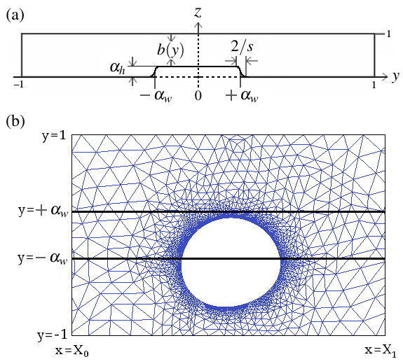
Fig.  3: (a) Cross-section of the channel including a rail with relative width $\alpha_{w}$, relative height $\alpha_{h}$ and sharpness $s$. The channel depth profile is given by $b(y)$. (b) Top view of the channel, showing a typical finite element mesh and bubble contour. Solid black lines at $\alpha_{w}$ and $-\alpha_{w}$ represent the edges of the rail. Both (a) and (b) are plotted in a dimensionless coordinate system.

We model the motion of finite bubbles on a rail by extending our two-dimensional lubrication model²⁰, initially developed to describe propagation of air fingers (open-ended bubbles) in similar channels. The model described below was later shown to be quantitatively accurate in channels of sufficiently large aspect ratio $\alpha\geq 40$, for thin rails with $\alpha_{h}<0.12$, and moderate values of the capillary number $Ca<0.012$¹⁹.

The geometry of a typical channel cross-section is shown in figure 3a. We introduce a Cartesian coordinate system aligned with the channel such that $x$ is the axial coordinate and $y$ and $z$ span the cross-section. The $x$ and $y$ (width) coordinates have been non-dimensionalised by $W^{*}/2$, whereas the $z$ coordinate (height) has been non-dimensionalised by $H^{*}$. The rail is represented by a smooth tanh-profile leading to a channel depth profile of the form

$$b(y)=1-\frac{\alpha_{h}}{2}[\tanh s(y+\alpha_{w})-\tanh s(y-\alpha_{w})],$$ (1)

where $s$ is the sharpness of profile edges, $\alpha_{h}=h^{*}/H^{*}$ is the fractional height of the obstacle, and $\alpha_{w}$ is the fractional width of the rail at half its maximum height.

We define a reference velocity scale as $U_{0}^{*}=Q^{*}/(W^{*}H^{*})$, and non-dimensionalise the depth-averaged horizontal velocity $\bf{u^{*}}$ on the scale $U_{0}^{*}$, pressure $p^{*}$ on the scale $6\alpha\mu^{*}U_{0}^{*}/(H_{0}^{*})^{2}$ and time on the scale $W^{*}/(2U_{0}^{*})$.

After applying the lubrication approximation ²¹, the governing equation for the viscous, incompressible fluid in the frame of reference moving with the bubble tip $\mathbf{U}_{b}=(U_{b},0)$, where $U_{b}=U_{b}^{*}/U_{0}^{*}$, is

$$\bm{u}=-b^{2}\bm{\nabla}p,\quad\bm{\nabla}\cdot(b(y)^{3}\bm{\nabla}p)=0\quad\mathrm{in}\quad\Omega,$$ (2)

where $\Omega$ denotes the fluid domain. The fluid domain is $X_{0}\leq x\leq X_{1}$, $-1\leq y\leq 1$, excluding the region occupied by the bubble, where $X_{0}$ and $X_{1}$ are truncation coordinates behind and ahead of the centre of the bubble (figure 3b).

The conditions at the bubble interface $\mathbf{R}=(x,y)$ and on the channel boundaries are

$$p_{b}-p=\frac{1}{3\alpha Q}\left(\frac{1}{b(y)}+\frac{\kappa}{\alpha}\right)\quad\mathrm{on}\quad\partial\Omega_{b},$$ (3)

$${\bf\hat{n}}\cdot\frac{\partial\mathbf{R}}{\partial t}+{\bf\hat{n}}\cdot\mathbf{U_{b}}+b^{2}{\bf\hat{n}}\cdot\bm{\nabla}p=0\quad\mathrm{on}\quad\partial\Omega_{b},$$ (4)

$$\frac{\partial p}{\partial y}=0\quad\mathrm{on}\quad y=\pm 1.$$ (5)

where $\partial\Omega_{b}$ denotes the bubble boundary with unit normal ${\bf\hat{n}}$ directed into the fluid.

The dynamic boundary condition (3) is the non-dimensional form of the Young-Laplace equation, where $p_{b}$ is the pressure inside the bubble, $Q=\mu^{*}U_{0}^{*}/\sigma^{*}$ is the dimensionless flow rate based on the net volume flux, and $\kappa$ is the dimensionless curvature of the interface in the $(x,y)$ plane. We assume for both kinematic and dynamic boundary conditions that the bubble occupies the full height of the channel, which neglects the effects of the thin films known to develop above and below the bubble.

The interfacial conditions in the moving frame have been previously derived¹⁹ and the only difference from the interfacial conditions in the fixed lab frame²⁰, is in equation (4), which adds the velocity of the frame moving with the tip of the bubble, $\mathbf{u}=-\mathbf{U}_{b}-b^{2}\bm{\nabla}p$, into the kinematic boundary condition $\displaystyle{\frac{\partial\mathbf{R}}{\partial t}\cdot\mathbf{\hat{n}}=\mathbf{u}\cdot\mathbf{\hat{n}}}$.

In the experiments, the control parameter is the volume flux $Q^{*}$ imposed by the syringe pump. In the model, we set the fluid pressure to zero at the rear of the domain, and applying a pressure gradient $-\Lambda\bf{e}_{x}$ far ahead of the bubble tip, where the value of $\Lambda$ is chosen to satisfy the dimensionless volume constraint:

$$\frac{1}{2}\int_{-1}^{1}b(y)\mathbf{u}\cdot\mathbf{e}_{x}\,\mathrm{d}y=1.$$ (6)

By recalling that $\mathbf{u}\cdot\mathbf{e}_{x}=-b^{2}p_{x}\rightarrow-b^{2}\Lambda$, we can in fact solve for $\Lambda$ in terms of an integral:

$$\Lambda=\frac{2}{\int_{-1}^{1}b^{3}(y)\,\mathrm{d}y}.$$ (7)

The dimensionless constant $\Lambda$ is a function of channel geometry only, taking the value $1$ for a rectangular channel, and increasing with obstacle height.

The dynamic boundary condition (3) does not include the correction factor of $\pi/4$ first derived by Park and Homsy ²² required to match to the static solution in large aspect-ratio channels in the absence of any depth variations. A constant factor of this form can be accommodated within our model by rescaling $\alpha$ and $Q$ as discussed by Franco-Gómez et al. ¹⁹, and so would not qualitatively alter the results; however Franco-Gómez et al. found that its inclusion actually increased the error between model results and the experimental data for air fingers at the typical flowrates considered here. A bigger difficulty is that the correction factor itself could be altered by the presence of the rail and the flow rate, and can display significant spatial variation even without topographic variations ²³. In principle, we could dynamically adjust the curvature term according to measured film thicknesses, but this is not a predictive model and is complicated by the existence of multiple solutions for bubble shape and hence for film thickness. Any such adjustment would therefore be somewhat ad hoc and we prefer to keep the model as simple as possible in order to explore underlying mechanisms, rather than pursuing exact quantitative agreement. Nevertheless, we should remark that de Lózar et al. ²⁴ did find quantitative agreement between the uncorrected model presented here and three-dimensional Stokes flow simulations of air fingers for channel aspect ratios greater than or equal to $8$ and capillary numbers above $0.01$, for channels without obstacles.

A second adjustment to the basic depth-averaged model that has been proposed²⁵ is the use of Brinkman equations, involving the ad-hoc inclusion of higher order lateral diffusion terms. The advantage of the Brinkman equations is that both the no-slip boundary condition on the wall and the tangential stress boundary condition on the bubble boundary can be satisfied. The bubble diameters considered here are much smaller than the channel width, so wall slip is unlikely to be significant. However, it is unclear how significant the tangential stress boundary layer would be, nor is it clear how the Brinkman equations should be modified by the presence of the obstacle. Again, we will omit Brinkman terms here for the sake of simplicity; the question of the validity of various depth-averaged models, the importance of dynamic film thickness, and how these interact with topographic variations, would best be explored by detailed full three-dimensional numerical computations.

The term $\partial\mathbf{R}/\partial t$ is the only time derivative in the problem and drives the unsteady evolution of the bubble. In this work we focus on steady solutions computed by setting $\partial\mathbf{R}/\partial t=0$, but we also present results using time-dependent simulations in figures 9, 12 and 13. Note that the time-derivative term also features in the stability analysis of the steady states.

The bubble velocity $U_{b}$ is an unknown with the associated constraint that the centroid of the bubble is fixed at $x=0$. The fluid pressure is fixed to zero far ahead of the bubble, which means that the bubble pressure $p_{b}$ is also an unknown with the associated constraint that the bubble volume must remain a prescribed constant, $V_{0}$, during the evolution

$$\iint_{\Omega_{b}}b(y)\mbox{d}A=V_{0},$$ (8)

assuming that the bubble occupies the full height of the channel. Note that the numerical values for $y_{c}$ are calculated using the height-weighted centroid position (see Supplementary Material); this differs from the experimental definition by at most 1.1%.

The model is solved using the finite element library oomph-lib²⁶ and implementation details are given in the supplementary material as well as in our previous papers ^{20, 19}.

4 Results

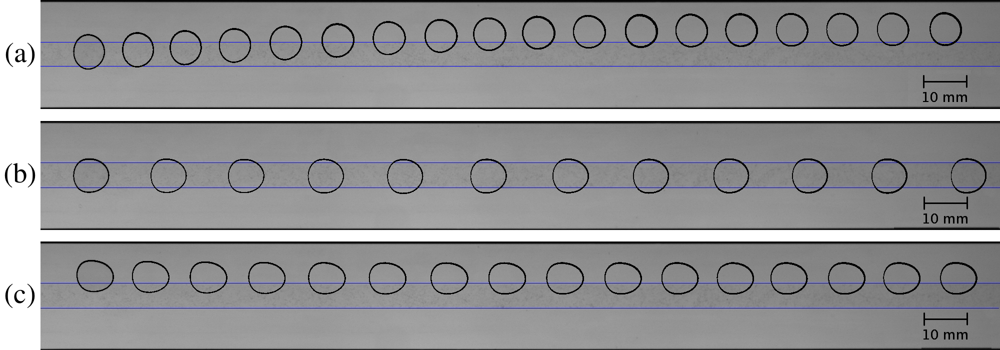
Fig.  4: Time-lag images of a propagating bubble with diameter $D=D^{*}/w^{*}=1.33$ in a channel with aspect ratio $\alpha=30$, rail width $w^{*}=6.9\pm 0.1$ mm and rail height $h^{*}=24.0$ $\mu$m. The solid blue lines delineate the edges of the rail. (a) $Q^{*}=3.0$ ml/min: the bubble starts in the on-rail position and is displaced towards an off-rail stable state (images taken every $5$ s) . (b) $Q^{*}=19.0$ ml/min: the bubble starts in the on-rail position and propagates on-rail (images taken every $1$ s). (c) $Q^{*}=13.0$ ml/min: the bubble starts in the off-rail position and propagates off-rail (snapshots every $1$ s).

4.1 On and off-rail bubble propagation

As described in the introduction, in a channel of uniform depth bubbles are transported along the centreline ($y=0$) of the channel ^{27, 4} and adopt states that are symmetric about the centreline. In contrast, we have found that the introduction of a thin rail along the bottom of the channel enables three modes of propagation: an on-rail symmetric mode analogous to bubble propagation in channels of uniform depth; and two asymmetric off-rail modes, one on each side of the rail. In a given experimental system, only one of the off-rail modes is generally observed, as illustrated in figure 4, because of a small, unavoidable bias in the experimental channel.

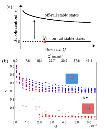
Fig.  5: (a) Schematic diagram summarising the experimental observations illustrated in figure 4. (b) Quantitative data corresponding to the schematic diagram: the centroid position $y_{c}=2y^{*}_{c}/W^{*}$ of steadily propagating bubbles of different sizes as a function of flow rate $Q^{*}$ in the experimental channel with a rail of width $w^{*}=6.9\pm 0.1$ mm and height $h^{*}=24.0$ $\mu$m. The bubble size is quantified by the diameter of the bubble at rest, relative to the width of the rail, $D=D^{*}/w^{*}$, in the on-rail position: ($\bigstar$) $D=0.77$, ($\blacktriangledown$) $D=1.04$, ($\bullet$) $D=1.33$, ($\blacksquare$) $D=1.65$ and ($\blacktriangle$) $D=1.81$. Red (blue) symbols correspond to initial conditions being on-rail (off-rail). Open symbols denote experiments where a steadily propagating state was not reached within the length of the channel. The cluster of open stars in the vicinity of $y_{c}=0$ denote experiments on the smallest bubble with $D=0.77$, for which a steady on-rail state was not observed, but where the migration towards the off-rail state was very slow.

The stability of the different propagation modes depends on the channel geometry, bubble size and flow rate, but the mode selected also depends on the initial conditions. If a bubble of diameter $D=D^{*}/w^{*}=1.33$ is started from an on-rail position, it migrates towards an off-rail position for low flow rates (figure 4a), whereas above a critical flow rate $Q_{c}$, the bubble propagates steadily on the rail (figure 4b). By contrast, if started in an off-rail position, the bubble is transported steadily in an off-rail position for all values of $Q$ investigated (figure 4c). Hence, for $Q>Q_{c}$, the device exhibits bistability, with on-rail (off-rail) propagation reached from on-rail (off-rail) initial conditions, respectively, while for $Q<Q_{c}$, the on-rail mode of bubble propagation is unstable. This scenario is summarised in a schematic bifurcation diagram in figure 5a.

Quantification of the existence of the on and off-rail modes of propagation is provided in figure 5b, where the centroid position $y_{c}$ of steadily propagating bubbles is plotted as a function of flow rate for a range of static bubble diameters relative to the rail width, $0.77<D=D^{*}/w^{*}<1.81$, for the case of rail width $w^{*}=6.9$ mm. Red (blue) symbols correspond to on-rail (off-rail) initial conditions, respectively. For off-rail initial conditions all bubbles propagated in the steady off-rail state. For on-rail initial conditions, the smallest bubble $D=0.77$ does not attain a steadily propagating state. Bubbles with $1.04\leq D\leq 1.65$ propagate steadily on the rail for sufficiently large flow rates. The largest bubble $D=1.81$ did not propagate steadily on the rail, but instead rapidly migrated sideways to attain a steady off-rail propagation state (figure 4a). Open symbols indicate bubbles that have not reached a steady state within the visualisation window. In the main, these are bubbles near the stability threshold, with the exception of the smallest bubble, $D=0.77$, for which the migration to an off-rail state was very slow.

4.2 On-rail stability tongues: a concept for sorting bubbles by size

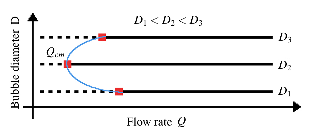
Fig.  6: Schematic diagram summarising the stability of the on-rail mode of propagation as a function of flow rate for three different bubble diameters. The red squares indicate the critical flow $Q_{c}$ rate beyond which the on-rail mode is stable for each bubble. The variation of $Q_{c}$ with bubble diameter observed in figure 5 is non-monotonic, resulting in a tongue-shaped stability boundary between unstable and stable on-rail modes in the parameter plane spanned by bubble diameter and flow rate. The minimum value of the critical flow rate $Q_{cm}$ occurs for an intermediate bubble size.

Figure 5b suggests that $Q_{c}$, the smallest value of flow rate for which an initially centred bubble remains on the rail during propagation to the end of the channel, varies non-monotonically with bubble diameter. Inspection of the data suggests a tongue-shaped stability boundary in the parameter plane spanning bubble diameter and flow rate, with a minimum value of the critical flow rate, $Q_{cm}$, for an intermediate bubble size, illustrated schematically in figure 6. Hence, for a flow rate marginally larger than $Q_{cm}$, only those bubbles within a narrow band of sizes can propagate steadily on-rail; bubbles of other sizes will migrate to off-rail positions.

The experimental stability boundaries, showing $Q_{c}$ as a function of bubble diameter, are presented in figure 7. The range of bubble diameters tested for $w^{*}=6.9$ mm (figure 7a) and $w^{*}=10.7$ mm (figure 7b) was $1.07\leq D\leq 1.65$ and $1.02\leq D\leq 1.39$, respectively. The stability boundaries demarcate regions of stable on-rail bubble propagation, which lie inside the tongues, from regions of stable off-rail propagation for bubbles set into motion in an on-rail position. Both graphs are qualitatively similar but exhibit different dimensional values of $Q_{cm}^{*}=14.7$ ml/min and $Q_{cm}^{*}=8.0$ ml/min associated with distinct (dimensional) bubble diameters $D=1.29$ ($D^{*}=8.94$ mm) and $D=1.13$ ($D^{*}=12.12$ mm), respectively. The increase in the dimensional size of the bubble at $Q_{cm}$ with the widening of the rail suggests that the band of bubble sizes that can be segregated through propagation on the rail can be tuned by varying the rail width.

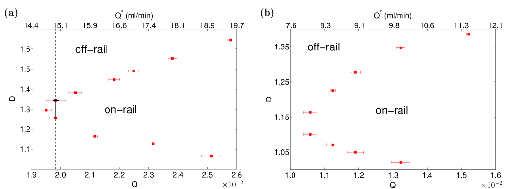
Fig.  7: Experimental stability boundaries in the parameter plane spanning bubble area and flow rate, which demarcate regions of bistability (inside the tongue) from regions of off-rail propagation (outside the tongue). (a) $w^{*}=6.9\pm 0.1$ mm, where $Q_{cm}^{*}=14.7$ ml/min for $D^{*}=8.94$ mm. The dashed line highlights the narrowest band of bubble diameters that may be stabilised robustly in this device. (b) $w^{*}=10.7\pm 0.1$ mm, where $Q_{cm}^{*}=8.0$ ml/min for $D^{*}=12.12$ mm.

For the smaller bubble diameters, the time required to reach a steady off-rail propagation mode from an on-rail initial condition, was generally found to increase as the bubble size decreased. For bubbles with $D=0.77$, a precise value of $Q_{c}^{*}$ could not be determined due to the length of the transient migration of the bubbles towards a steady state, but a study of the time evolution of the centroid position for increasing values of $Q^{*}$ suggests a value $43.0<Q_{c}^{*}<50$ ml/min. These long durations and thus extended lengths of migration could prevent the sorting of bubbles near the size thresholds in practical devices. In all cases, however, the duration of transient migration near the threshold $Q^{*}_{c}$ could be reduced by biasing the symmetric on-rail initial condition, thus enabling segregation by size in channels of finite length. For example, when the initial centroid displacement from the channel centreline was increased from the experimental tolerance of $500\;\mu$m to $1000\;\mu$m, the duration, and thus length, of transients were reduced by up to 40%.

Bubbles with larger diameters than those shown in figure 7, i.e. $D>1.65$ for $w^{*}=6.9$ mm, and $D>1.39$ for $w^{*}=10.7$ mm, did not propagate steadily on-rail. However, for bubbles large enough to span the entire width of the channel in the static configuration, $D\alpha_{w}\approx 1$, a symmetric (on-rail) propagation mode can be supported at low values of the flow rate; above a critical flow rate, this symmetric mode loses stability to a pair of asymmetric propagation states through either a supercritical or subcritical pitchfork bifurcation depending on the rail height ¹⁹. These observations highlight the complex dependence of the modes of propagation on the size of the bubble and hint at the rich nonlinear dynamics of bubble propagation exhibited by this system.

4.3 Comparison between experimental and numerical stability tongues

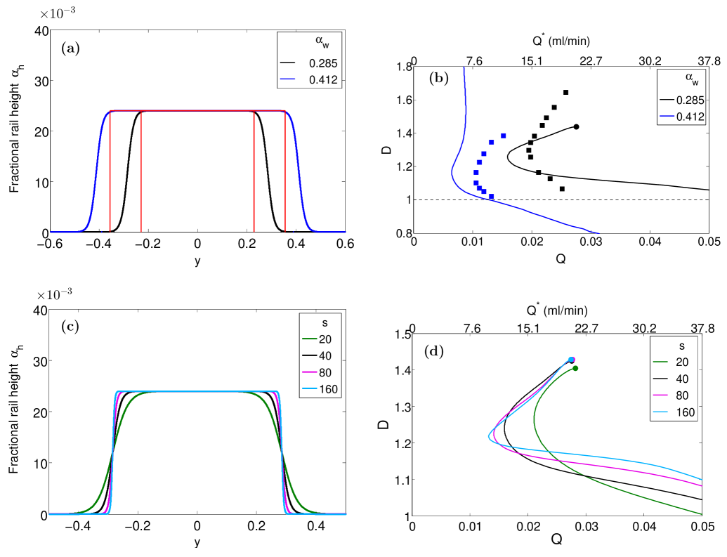
Fig.  8: (a) Comparison between the model rail profiles with $\alpha_{h}=0.024$, shown with thick solid lines ($\alpha_{w}=0.285$, $s=40$ (black), $\alpha_{w}=0.310$, $s=40$ (blue)), and the corresponding experimental rail profiles measured by profilometry (red lines). (b) Comparison for the rail geometries shown in (a) between the path of the pitchfork bifurcation that stabilises the on-rail mode of propagation (lines), plotted in the parameter plane spanned by flow rate and bubble diameter, and the experimental stability boundaries (symbols), previously plotted in figure 7. The horizontal dashed line marks the width of the rail, while the solid circles mark the ends of the pitchfork bifurcation paths, which are discussed in 4.4. (c) Model rail profiles with varying levels of sharpness with $\alpha_{w}=0.285$. (d) Paths of the pitchfork bifurcation corresponding to the rail profiles in (c), showing the sensitivity of the results to the sharpness of the rail.

We first evaluate the predictive capability of our depth-averaged model for finite bubbles with diameters ranging between one and two rail widths. The model has been shown to be quantitatively accurate when modelling air finger propagation in channels of larger aspect ratios, $\alpha\geq 40$, at relatively low flow rates, so that liquid films above and below the finger may be neglected¹⁹. In these simulations, the results were unaltered²⁰ for sufficiently sharp changes in channel depth, $s\geq 40$ in equation (1). In the present study, however, we cannot rely on the quantitative accuracy of the model because the steady on-rail state is stabilised at relatively large values of $Q$; the small finite bubbles used here may be more sensitive to details of the rail geometry than the long air fingers; and the aspect ratio is only $\alpha=30$. For large bubbles (with diameters approaching the channel width) at low flow rates ($Q\lesssim 0.01$), we have recently demonstrated quantitative agreement between the model and experimental data ²⁸

The rail height in the model was chosen based on micrometer measurements of the height of the experimental rail, so that $\alpha_{h}=0.024$. Measurements of the the height profile at six different locations along the rail length using a step profilometer (DekTak IIA), with a resolution of $0.1\mu$m (see Supplementary Material), are consistent with the micrometer measurements, but they indicate that the top surface of the rail is rough with a standard deviation of the height from its mean value of approximately $3\mu$m. Moreover, the profilometry measurements show that the sidewalls of the rails are approximately vertical. Hence, although we follow Franco-Gómez et al. ¹⁹ in choosing a rail sharpness of $s=40$, and choosing $\alpha_{w}$ in order to match the top width of the rail, we also present a sensitivity analysis of the stability of the on-rail mode of bubble propagation to increases in the value of $s$ at fixed $\alpha_{w}$ (see figure 8c,d).

Figure 8a shows the rail profiles used in the model when $s=40$ by comparison with the two experimental rail profiles based on micrometer measurements. The model predicts that for low flow rates the symmetric on-rail state is unstable and it gains stability via a pitchfork bifurcation at a critical value of the flow rate that depends on the bubble size, for a fixed channel geometry. Thus, the path of the pitchfork bifurcation should coincide with the boundary of the stability tongue found experimentally. Bifurcation-tracking calculations were performed to determine the location of this bifurcation as a function of bubble size, and numerical stability results are compared with experimental data in figure 8b. We find broad qualitative, but not quantitative, agreement. For example, the numerical simulations systematically underpredict the critical flow rates for stability, but as the width of the rail increases, the critical flow rates decrease in both the experiments and the model, as does the relative size of the bubble at minimum critical flow rate. The detailed bifurcation structure underlying on and off-rail propagation modes in the model is more complex than the results shown in figure 8b and will be discussed further in section 4.4.

For the narrower rail, the numerical computations yield a narrower stability tongue and a smaller minimum value of the critical flow rate than the experiments. Nonetheless, the bubble diameters corresponding to the minimum value of the critical flow rate agree to within 2% of the numerical value. In order to explore the sensitivity to the rail geometry, we adjusted the value of $s$ within the range $20\leq s\leq 160$, while keeping $\alpha_{w}$ constant – this is equivalent to maintaining the width of the obstacle between the two points corresponding to half the maximum height (see figure 8c). The paths of the pitchfork bifurcation corresponding to these profiles are shown in figure 8d. As $s$ increases, the paths converge towards a pointed triangular tongue shape which has a lower cutoff size that is only weakly dependent on flow rate, while the upper bound on drop size increases with flow rate. The experimental results show a much rounder tongue, reminiscent of the numerical results for smoother profiles.

For the wider rail, one aspect of the qualitative agreement is lost because, in the model, the path of the pitchfork bifurcation is such that larger bubbles remain stable above a critical flow rate. Hence, according to the model, the system no longer has a large-diameter cut-off. Nonetheless, the remnants of a tongue-like region remain and its approximate width is in better agreement with the experimental data than for the narrow rail.

A further comparison between experiment and model can be obtained by studying the transient evolution into the off-rail state. Figure 9 shows results for $y_{c}$ as a function of dimensionless time for a bubble with $D=1.33$ during its migration to an off-rail state at a low flow rate ($Q^{*}=3\,\mathrm{ml/min}$, $Q=4.0\times 10^{-3}$), and (a)-(f) shows snapshots of bubble shape during this transition. The timescales of bubble motion are in broad agreement, with the predicted migration being faster than the experiments by a factor of approximately 1.6, and the shapes are in reasonable agreement given the evident difference in timescales. The discrepancy in timescales reduces as flow rate is increased for the three cases we have data for, with factors of $1.2$ at $Q=6.6\times 10^{-3}$ and $1.0$ at $Q=9.3\times 10^{-3}$. The shapes shown in (g) and (h) in figure 9 correspond to steady propagation rather than transient migration, and also correspond to (b) and (c) in figure 4. The main difference between the observed and predicted shapes is that the predicted bubbles have smaller projected area, which will be discussed shortly.

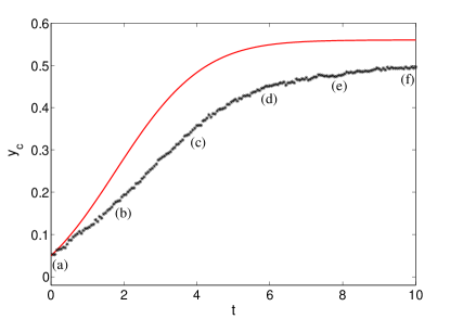
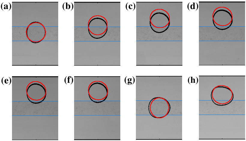
Fig.  9: Experiments (black) and model predictions (red line) for the evolution of bubble offset $y_{c}$ as a function of dimensionless time $t$. Here $D=1.33$ and $Q^{*}=3\,\mathrm{ml/min}$ ($Q=4.0\times 10^{-3}$). Snapshots (a)-(f) correspond to times indicated in the first plot. (g) and (h) show steady states for larger flow rates: $Q^{*}=19\,\mathrm{ml/min}$ ($Q=6.6\times 10^{-3}$) and $Q^{*}=13\,\mathrm{ml/min}$ ($Q=9.3\times 10^{-3}$) respectively. Sequences of experimental snapshots corresponding to (g) and (h) can be found in figure 4.

The numerical results presented in figures 8 and 9 suggest that the model captures the qualitative features of bubble propagation in the channel with a centred rail, and thus may be used as a design guide rather than a predictive tool. The depth-averaged lubrication model is convenient because it significantly reduces computational costs compared with a three-dimensional model based on the Navier–Stokes equations. It also dissociates the effect of the rail on the bulk viscous flow from its effect on surface tension forces through cross-sectional curvature variations which are accounted for in the dynamic boundary condition. This facilitates numerical investigation into the physical mechanisms of on-rail bubble propagation because the effect of the channel topography may be removed from either equation independently, as will be discussed in section 4.5. However, the quantitative discrepancies between the depth-averaged model and the experiment are most likely to be due to three-dimensional effects. Although the channel has an aspect ratio $\alpha=30$, the width to depth ratio of the confined bubbles is as low as $7$. Moreover, the depth-averaged model does not account for the liquid films that separate the bubble from the boundaries of the channel and the rail. For finger propagation, the presence of such films has been found to generate quantitative discrepancies with the model for comparable values of the non-dimensional flow rate investigated here ¹⁹.

Film thicknesses were estimated by measuring the increase in mean bubble diameter (relative to the static bubble diameter) with increasing flow rate, for a bubble that retains a constant volume. For $Q=2.50\times 10^{-2}$ (or $Q^{*}=19$ ml/min), which is a typical experimental flow rate in figure 8b,d, and also shown in figure 9g, the film thickness is approximately four times larger than the rail height (see Supplementary Material). This suggests that the bubble may not feel the solid rail but an effective rail profile covered by a fluid film. It also concurs with the stability results of figure 8b,d, which indicate that wider rails with gently sloping side walls are required to approximate the experimental measurements. Although it would be possible to apply an optimisation procedure to find an effective geometry for the depth-averaged model that best fits the experimental data, this does not lead to a predictive model. Hence, it appears that a detailed simulation of the thin films would be essential to achieve a quantitative prediction of the stability tongues. The feasibility of such simulations in the absence of rails where lateral symmetry can be assumed has recently been demonstrated²⁹, but the simulations remain too computationally expensive to conduct a detailed bifurcation analysis in reasonable time.

4.4 Bifurcation diagram

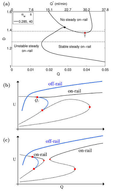
Fig.  10: (a) Bifurcation diagram for a channel with $\alpha=30$, $\alpha_{w}=0.285$, $\alpha_{h}=0.024$ and $s=40$ spanning flow rate and bubble diameter. The path of a pitchfork bifurcation separates regions of unstable and stable steady on-rail propagation. The path of a limit point encloses a region in which there are no steady on-rail states. Schematic bifurcation diagrams of the bubble speed as a function of flow rate are shown for two values of the bubble diameter indicated with dashed lines: (b) $D=1.27$ ($D^{*}=8.74$ mm) and (c) $D=1.37$ ($D^{*}=9.44$ mm). Solid (dashed) lines denote stable (unstable) solutions, while blue (black) lines denote off-rail (on-rail) states, respectively. In (b), the upper $\blacksquare$ denotes the pitchfork bifurcation point that stabilises the on-rail state. Upon the increase of the bubble diameter, the stable on-rail solution branch interacts with the unstable RVB solutions in the lower part of diagram (b), which results in its disconnection in (c) so that there is no simple steady on-rail solution in the region delimited by the upper two saddle node points $\bullet$ in (c), although the unstable RVB solution remains in the lower part of the diagram. The disconnection of the stable on-rail solution branch arises through a transcritical bifurcation at $D\approx$ 1.365 ($Q=0.039$), marked as T in (a).

The stabilisation of the symmetric on-rail propagation modes occurs via a symmetry-breaking pitchfork bifurcation, but an obvious question is what happens to this bifurcation for small and large bubbles. In other words: how is the stability of the on-rail solutions lost as the bubble size changes? From a dynamical systems point of view, the easiest scenario would be that the symmetry-breaking bifurcation rapidly moves to a very high flow rate as the critical bubble sizes are reached, leading to the parallel-sided tongue sketched in figure 6. In our model we do indeed find this to be the case for small bubble diameters, but the scenario for larger bubble sizes is more complex.

Figure 10a shows the results of steady bifurcation tracking calculations extending the results for the narrower rail ($s=40$, $\alpha_{h}=0.024$ and $\alpha_{w}=0.285$) shown in figure 8b. We find that there is a region, bounded by a path of limit points, where the steady on-rail solution previously investigated is completely absent. For large bubble diameters the pitchfork bifurcation is annihilated at this path of limit points at a finite value of the flow rate (black solid circle). In time-dependent simulations, we find that bubbles in the region in which there are no steady on-rail solution evolve until they reach a point at which they would be expected split into multiple bubbles, but bubble pinch-off is not included in our current model.

The gap in steady on-rail solutions can be further understood by considering the bubble velocities as functions of flow rate for all computed steady solutions at a fixed bubble size, see figures 10b,c, which correspond to $D=1.27$ and $D=1.37$, respectively. In figures 10b,c, solid (dashed) lines denote stable (unstable) propagation modes, and on-rail (off-rail) bubbles are shown with black (blue) lines, respectively. In both cases, the off-rail mode of propagation is stable for all values of $Q$. On-rail (symmetric) bubbles generally travel with lower speeds than the off-rail (asymmetric) bubbles because they are confined to a shallower channel over the rail, and thus viscous resistance is relatively increased. In figure 10b, the on-rail bubble is unstable for flow rates below a critical value $Q_{c}$ and stable above. In fact, the loss of stability of the stable on-rail bubble at $Q_{c}$, represented by a stability tongue as a function of bubble size in figure 10a, occurs through a subcritical pitchfork bifurcation at $Q_{c}$, where two unstable asymmetric branches emerge (these branches have the same bubble velocity $U$). These asymmetric solution branches connect via a second pitchfork bifurcation to another type of symmetric solution of lower bubble velocity. This symmetric solution is unstable, and exhibits the characteristically dimpled bubble tips of unstable Romero–Vanden-Broeck solutions (RVB) uncovered in the context of Saffman–Taylor fingering in Hele-Shaw channels ^{30, 31}. As the bubble size increases from $D=1.27$ to $D=1.37$, interaction between the stable on-rail solution branch and the unstable RVB solution branch leads to a transcritical exchange of stability at an intermediate value of $D$. A further increase in bubble size towards $D=1.37$ disconnects the transcritical bifurcation through the emergence of two limit points, which bound an interval of intermediate values of $Q$ where stable on-rail bubbles are not found, as illustrated in figure 10c. The variation of these limit points with increasing bubble size form the stability boundary in figure 10a that encloses the ‘no steady on-rail’ region. As the bubble size increases further the two pitchforks move closer together and annihilate each other as they interact with the limit point.

4.5 Physical mechanism of on-rail propagation

We now investigate the physical mechanisms that enable on-rail bubble propagation. For consistency with the numerical results, we shall describe the mechanisms via the depth-averaged model described in section 3. In this framework, the deformation of the bubble is driven by the kinematic condition, equation (4), and in the lab frame the normal velocity is given by the term $-b^{2}{\bf\hat{n}}\cdot\bm{\nabla}p$. Hence the behaviour of the bubble can be inferred from the local pressure gradients and channel depth. Note that the depth-averaged velocity profile that results from this model in the absence of obstacles and bubbles is uniform and not parabolic.

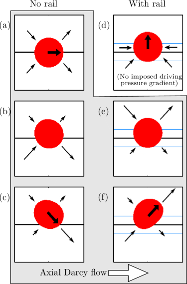
Fig.  11: Schematic diagram of migration mechanisms in an unoccluded Hele-Shaw cell (a)–(c) and in presence of a rail (d)–(f). The system is subject to an imposed pressure gradient driving a net flow from left to right in all cases except (d). Small arrows are normal velocity vectors and the large arrow indicates net direction of travel of the bubble. The centreline is shown as a solid line and in (d)–(f) the limits of the centred rail are shown as dotted lines. (a) Symmetric velocity field for a centred bubble. (b) Displacing the bubble reduces the normal pressure gradients and hence the normal velocities on the side of the bubble nearest the side wall, which leads to a net inclination of the bubble shown in (c). The surface-tension-induced pressure jump serves to enhance the pressure gradients, and hence normal velocities, near the tips, driving propagation in the direction of inclination: back towards the centreline. If there is no imposed driving pressure gradient (d), the presence of the rail leads to an increased cross-sectional curvature, which locally lowers the fluid pressure leading to positive pressure gradients away from the bubble and hence normal velocities over the rail directed towards the bubble, as shown. These drive net migration into the side channel. (e) Displacing the bubble when the rail is present leads to a net increase in normal velocities on the side of the bubble nearer the wall owing to the presence of the deeper side channels, provided that the increase in depth is sufficient to overcome the reduction in normal pressure gradient described in (b). The higher velocities nearer the wall lead to a net inclination of the bubble towards the side channel shown in (f), in the opposite direction to that in the unoccluded case (c). Thus, in this case when the bubble migrates in the direction of inclination it moves into the side channel.

In unoccluded Hele-Shaw cells an interaction between viscous and capillary effects underlies the dynamic mechanism that acts to return off-centre bubbles to the centreline. An initially circular bubble (when viewed from above) travelling along the centreline of an unoccluded Hele-Shaw call is driven by pressure and velocity fields that are symmetric about the centreline, which induce a symmetric deformation, see figure 11a. For small bubbles, this results in a slight decrease in the in-plane curvature (when viewed from above) at the front of the bubble and an increase in the in-plane curvature at the rear. If the bubble is displaced from the centreline, the magnitude of the pressure gradients normal to the bubble will decrease on the side of the bubble nearest the side walls where $\partial p/\partial y=0$, see figure 11b. The ensuing asymmetric velocity field will cause the bubble to incline relative to the centreline such that the point of maximum in-plane curvature at the rear moves towards the sidewall and the point of minimum in-plane curvature at the front moves towards the centreline, i.e. the bubble “points” towards the centreline, see figure 11c. The surface-tension-induced pressure jump over the interface means that the fluid pressure adjacent to the bubble will be lowest at point of maximum curvature and highest at the point of minimum curvature, which increases the magnitudes of the local pressure gradients and hence drives the bubble in the direction of inclination, eventually returning the bubble to the centreline.

Outside the depth-averaged framework the no-slip boundary condition on the channel walls leads to a non-uniform velocity profile with the fastest flow along the channel centreline. The velocity profile causes a bubble displaced from the centreline to incline in the same direction as a displaced bubble in the depth-averaged model and subsequently the same mechanism drives the conventional migration towards the centreline for Stokes flows in unoccluded channels ^{17, 18}. The propagation of bubbles in the direction of inclination has also recently been implicated as a key mechanism in Leonardo’s paradox: the onset of zigzag or helical trajectories for rising bubbles in still liquid³². These migration effects do not occur for rigid particles because they do not change their shape in response to the velocity field. We remark that the interaction between deformation and capillary-induced pressure jump is essential for the mechanism to operate.

The introduction of a rail alters both capillary forces via changes in cross-sectional curvature and also viscous forces via changes to the bulk resistance of the channel. Thus, we should expect the restoring mechanism just described to be disrupted for sufficiently large rails. In order to investigate the physical mechanisms leading to the migration of bubbles in the presence of the rail, we conducted a number of time-dependent simulations, selecting which terms are affected by the rail. For this numerical experiment, we chose the narrow rail, a fixed bubble size ($D=1.27$), a fixed flow rate ($Q=2.60\times 10^{-2}$), and a range of initial centroid positions. The results are shown in figure 12, where the centroid position $y_{c}$ of the bubble is shown as a function of time.

In figure 12a, cross-sectional depth variations in the channel are retained both in the bulk equations (2, 4) and in the dynamic boundary condition (3). Only a nearly symmetric initial bubble placement ($|y_{ci}|\leq 0.06$) results in stable on-rail bubble propagation; in other words, the basin of attraction of this stable solution is relatively small. As expected, the duration of transient migration is greatest for initial conditions near the basin boundary value of $y_{ci}$ separating stable on and off-rail bubble propagation. In figure 12b, the effect of depth variation is removed in the bulk equations (2,4) by setting $b(y)=1$, but the depth-profile is retained in the dynamic boundary condition (3). Removal of the variations in viscous resistance more than doubles the range of initial centroid positions ($|y_{ci}|\leq 0.15$) for which stable on-rail propagation is achieved. Hence, depth variations in the bulk enhances destabilisation of on-rail states. Finally, in figure 12c, the effect of cross-sectional depth variations is retained in the bulk but not in the dynamic boundary condition by setting $b(y)=1$ in eq. (3). In this case, all initial bubble positions lead to stable off-rail propagation. This demonstrates that the cross-sectional curvature variation introduced by the depth profile is essential to promote stable on-rail propagation for the system at these particular parameter values; a rather surprising result given that the very same curvature variation is responsible for destabilisation of the static bubble.

Fig.  12: Bubble centroid position (y-coordinate) as a function of nondimensional time from time-dependent numerical simulations. The channel parameters parameters are $\alpha=30$, $\alpha_{w}=0.285$ (narrow rail), $\alpha_{h}=0.024$ and $s=40$. The bubble has diameter $D=1.27$ ($D^{*}=8.74$ mm) and propagates with a fixed flow rate of $Q=2.60\times 10^{-2}$ ($Q^{*}=20$ ml/min), but note that we conduct this numerical experiment at fixed pressure gradient. (a) The prescribed channel depth variation $b(y)$ is included in both the bulk equations (2,4) and the dynamic boundary condition (3). The bubble remains on-rail for initial centroid positions $y_{c}\leq 0.06$ ($6$ %) and the steady-state off-rail position is $y_{c}=0.405$. (b) The prescribed depth variation is retained in the dynamic boundary condition but removed from the bulk equations by setting $b(y)=1$. The bubble remains on-rail for initial centroid positions $y_{c}\leq 0.15$ ($15$ %) and the steady-state off-rail position is $y_{c}=0.333$. (c) The prescribed depth variation is retained in the bulk equations but removed from the dynamic boundary condition by setting $b(y)=1$. The bubble migrates to an off-rail steady state with $y_{c}=0.369$ for all initial centroid positions.

Thus, the variation of viscous resistance caused by introduction of the rail in the absence of changes in cross-sectional curvature may lead to destabilisation of the on-rail propagation mode and eventual migration towards the off-rail propagation modes, despite the fact that the on-rail propagation mode is not significantly different from that shown in figure 11a. The non-uniform viscous resistance means that for a constant axial pressure gradient the velocity is faster in the off-rail regions, see figure 11e. If the bubble is displaced from the centreline and partially enters the off-rail region then the resulting speed differential over the interface will cause it to incline relative to the centreline so that it appears to be directed into the off-rail region, see figure 11f. The surface-tension-induced pressure jumps over the interface will again cause the bubble to migrate in the direction of inclination, which is now towards the off-rail region. As the bubble moves laterally more of the interface enters the off-rail region and travels at the higher speed, meaning that the bubble will become less inclined. Thus, the lateral propagation velocity decreases until the stable off-rail propagation mode is reached. If the viscous resistance remains uniform then this destabilisation mechanism is absent, which explains why the basin of attraction of the on-rail state increases in this case. For the parameters chosen in figure 12 we find that by reducing the rail height to less than one third of its former value, the standard centering mechanism is able to overcome these effects of bulk variation, and the on-rail state is again stabilised.

In the absence of flow, the increased cross-sectional curvature caused by confinement leads to locally lower pressures near the regions of the interface over the rail. The resulting pressure gradients drive flows that destabilise a bubble displaced from the centreline, which moves into an off-rail position, see figure 11d. If there is no variation in the viscous resistance, however, then in the presence of flow, as in the unoccluded channel, the bubble inclines so that its tip is nearer the centreline, which acts to drive the bubble towards an on-rail position. Thus, the capillary-driven and viscous-pressure-driven flows act in opposite directions near the downstream end of the bubble; compare the arrows on the right-hand-side of the bubbles in figures 11c and 11d. Hence, for sufficiently large flow rates, the on-rail position is always stabilised when there is no variation in viscous resistance.

When variations in depth are included in both bulk equations and interfacial boundary conditions then the final direction of inclination of the bubble caused by the interplay between viscous and capillary effects, and hence stability of the on-rail state, depends crucially on the bubble size and position, which gives rise to the observed complex behaviour for which we have no simpler predictive model than solving the full set of two-dimensional governing equations.

The time-dependent numerical simulations shown in figure 12a were repeated for a wide range of bubble sizes. Figure 13 shows the largest initial off-centre centroid position $y_{ci}^{\mathrm{m}ax}$ for which stable on-rail propagation occurs as a function of bubble size, within the range of bubble sizes for which stable on-rail propagation could be achieved. The variation of $y_{ci}^{\mathrm{m}ax}$ is small and there is a sudden drop in $y_{ci}^{\mathrm{m}ax}$ at $D=1.12$ and $D=1.41$ which are the smallest and largest bubble sizes that allow stable on-rail propagation, respectively. This suggests that the sensitivity to positioning perturbations remains essentially constant within the stability tongues previously shown in figure 8b.

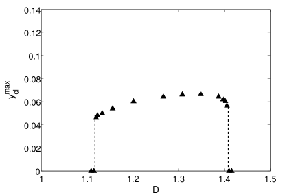
Fig.  13: Maximum initial centroid position allowing a bubble to return to a stable on-rail propagation mode as a function of bubble diameter in the numerical simulations. The flow rate and channel parameters are the same as in figure 12.

5 Conclusions

The transport of bubbles, capsules and droplets by driving carrier fluid within a confined geometry is a universal process in industry and nature. The channel geometry influences the possible propagation modes and for a large-aspect-ratio rectangular channel, or Hele-Shaw cell, the solution structure is particularly rich ^{33, 34}. A panoply of different propagation modes has been uncovered, but for Hele-Shaw channels without rails or grooves, the vast majority of these modes are unstable and the only observed propagation mode is centred and symmetric about the channel’s centreline.

In the present paper, we find that introduction of a rail on the base of the channel introduces stable asymmetric, off-rail propagation modes for all flow rates and bubble sizes considered. In contrast, the centred, on-rail propagation modes are only stable for a limited range of bubble sizes and above a minimum flow rate $Q_{cm}$. Thus, bubbles within a narrow size band may be segregated from others by fixing the flow rate at a value marginally larger than $Q_{cm}$. Under these conditions, the propagation of a train of bubbles of different sizes, which are sufficiently separated to avoid bubble interactions, will result in only those bubbles within the band remaining on the rail after reaching a steady propagation state. Both smaller and larger bubbles will migrate into the side channels allowing their removal from the main stream as illustrated schematically in figure 1. The experiments presented in this paper were performed with quasi-static initial conditions, but in practice, bubbles propagating steadily in a channel of rectangular cross-section would be centred ^{18, 4}, and they could thus encounter the rail at a small distance downstream of the inlet of the channel, where segregation would occur.

In contrast to transport along grooves ¹¹, which relies on stabilisation of the capillary static solution, the present mechanism is dynamic, requiring sufficiently large viscous restoring forces to compensate for destabilising capillary-driven flows. The restoring mechanism is subtle, however, because both capillary and viscous forces can act as destabilising or stabilising in different regimes. The mechanism relies on an interplay between the viscous pressure gradient and surface-tension-induced capillary pressure drop, which leads to a critical flow rate for stable on-rail propagation that is not a monotonic function of bubble size.

We have restricted attention to bubbles of a comparable size to the rail width. As the bubbles increase in size and eventually interact with the sidewalls of the channel then they can no longer be segregated using this mechanism. In fact, large bubbles in Hele-Shaw cells under the introduction of a rail exhibit different but equally complex behaviour, similar to that of air fingers ¹⁹. Their dynamics are currently under investigation.

6 Acknowledgements

A.F-G. was funded by CONICYT. We thank Pallav Kant for performing the profilometry measurements of the thin-film rail, and Lucie Ducloué for helpful discussions. This work was supported by the Leverhulme Trust (Grant RPG-2014-081) and EPSRC (Grant EP/P026044/1).

References

- Xi et al. 2017 H.-D. Xi, H. Zheng, W. Guo, A. M. Ganan-Calvo, Y. Ai, C.-W. Tsao, J. Zhou, W. Li, Y. Huang, N.-T. Nguyen and S. H. Tan, Lab Chip, 2017, 17, 751–771.
- Piyasena and Graves 2014 M. E. Piyasena and S. W. Graves, Lab Chip, 2014, 14, 1044–1059.
- Leal 1980 L. G. Leal, Annu. Rev. Fluid Mech, 1980, 12, 435–476.
- Stan et al. 2011 C. A. Stan, L. Guglielmini, A. K. Ellerbee, D. Caviezel, H. A. Stone and G. M. Whitesides, Phys. Rev. E, 2011, 84, 036302.
- Di Carlo et al. 2007 D. Di Carlo, D. Irimia, R. G. Tompkins and M. Toner, PNAS., 2007, 104, 18892–18897.
- Kim et al. 2014 J. Kim, J. Erath, A. Rodriguez and C. Yang, Lab Chip., 2014, 14, 2480–2490.
- Cox and Mason 1971 R. G. Cox and S. G. Mason, Annu. Rev. Fluid Mech, 1971, 3, 291–316.
- Amini et al. 2014 H. Amini, W. Lee and D. Di Carlo, Lab Chip., 2014, 14, 2739–2761.
- Di Carlo 2009 D. Di Carlo, Lab Chip, 2009, 9, 3038–3046.
- Karnis and Mason 1967 A. Karnis and S. G. Mason, J. Colloid Interface Sci., 1967, 24, 164–169.
- Abbyad et al. 2011 P. Abbyad, R. Dangla, A. Alexandrou and C. N. Baroud, Lab Chip., 2011, 11, 813–821.
- Yamada et al. 2014 A. Yamada, S. Lee, P. Bassereau and C. Baroud, Soft Matter, 2014, 10, 5878–5885.
- Yoon et al. 2014 D. H. Yoon, S. Numakunai, A. Nakahara, T. Sekiguchi and S. Shoji, RSC Adv., 2014, 4, 37721–37725.
- Dawson et al. 2013 G. Dawson, S. Lee and A. Juel, J. Fluid Mech., 2013, 722, 437–460.
- Sciambi and Abate 2015 A. Sciambi and A. R. Abate, Lab Chip, 2015, 15, 47–51.
- Tanveer and Saffman 1987 S. Tanveer and P. G. Saffman, Phys. Fluids, 1987, 30, 2624–2635.
- Richardson 1973 S. Richardson, J. Fluid Mech., 1973, 58, 115–127.
- Chan and Leal 1979 P. C.-H. Chan and L. G. Leal, J. Fluid Mech., 1979, 92, 131–170.
- Franco-Gómez et al. 2016 A. Franco-Gómez, A. B. Thompson, A. L. Hazel and A. Juel, J. Fluid Mech., 2016, 794, 343–368.
- Thompson et al. 2014 A. B. Thompson, A. Juel and A. L. Hazel, J. Fluid Mech., 2014, 746, 123–164.
- Reynolds 1886 O. Reynolds, Phil. Trans. R. Soc., 1886, 177, 157–234.
- Park and Homsy 1984 C. W. Park and G. M. Homsy, J. Fluid Mech., 1984, 139, 291–308.
- Zhu and Gallaire 2016 L. Zhu and F. Gallaire, J. Fluid Mech., 2016, 798, 955–969.
- de Lózar et al. 2008 A. de Lózar, A. Juel and A. L. Hazel, J. Fluid Mech., 2008, 614, 173–195.
- Nagel et al. 2014 M. Nagel, P.-T. Brun and F. Gallaire, Phys. Fluids, 2014, 26, 032002.
- Heil and Hazel 2006 M. Heil and A. L. Hazel, Lecture Notes on Computational Science and Engineering. Springer, 2006, 53, 19–49.
- Goldsmith and Mason 1962 H. Goldsmith and S. Mason, J. Colloid Sci., 1962, 17, 448 – 476.
- Franco-Gómez et al. 2017 A. Franco-Gómez, A. B. Thompson, A. L. Hazel and A. Juel, Propagation of a finite bubble in a Hele-Shaw channel of variable depth., Submitted to Fluid Dyn. Res., 2017.
- Ling et al. 2016 Y. Ling, J.-M. Fullana, S. Popinet and C. Josserand, Phys. Fluids, 2016, 28, 062001.
- Romero 1982 L. A. Romero, PhD thesis, California Institute of Technology, 1982.
- Vanden-Broeck 1983 J. M. Vanden-Broeck, Phys. Fluids, 1983, 26, 2033–2034.
- Cano-Lozano et al. 2016 J. C. Cano-Lozano, C. Martínez-Bazán, J. Magnaudet and J. Tchoufag, Phys. Rev. Fluids, 2016, 1, 053604.
- Tanveer 1987 S. Tanveer, Phys. Fluids, 1987, 30, 651–658.
- Kopf-Sill and Homsy 1988 A. R. Kopf-Sill and G. M. Homsy, Phys. Fluids, 1988, 31, 18–26.