Teleportation simulation of bosonic Gaussian channels:
Strong and uniform convergence

Abstract

We consider the Braunstein-Kimble protocol for continuous variable teleportation and its application for the simulation of bosonic channels. We discuss the convergence properties of this protocol under various topologies (strong, uniform, and bounded-uniform) clarifying some typical misinterpretations in the literature. We then show that the teleportation simulation of an arbitrary single-mode Gaussian channel is uniformly convergent to the channel if and only if its noise matrix has full rank. The various forms of convergence are then discussed within adaptive protocols, where the simulation error must be propagated to the output of the protocol by means of a “peeling” argument, following techniques from PLOB [arXiv:1510.08863]. Finally, as an application of the peeling argument and the various topologies of convergence, we provide complete rigorous proofs for recently-claimed strong converse bounds for private communication over Gaussian channels.

I Introduction

Quantum teleportation Tele1 ; Tele2 ; telereview ; oldrev ; teleCV2 is a fundamental operation in quantum information theory NielsenChuang ; CVbook ; RMP and quantum Shannon theory HolevoBOOK ; Hayashi . It is a central tool for simulating quantum channels with direct applications to quantum/private communications TQC and quantum metrology ReviewMETRO . In a seminal paper, Bennett et al. ref1 showed how to simulate Pauli channels and reduce quantum communication protocols into entanglement distillation. Similar ideas can be found in a number of other investigations ref2 ; ref3 ; ref4 ; ref5 ; ref6 ; ref7 ; ref8 ; ref9 ; ref10 ; ref11 ; ref12 ; ref13 ; ref14 ; ref15 (see Ref. (TQC, , Sec. IX) for a detailed discussion of the literature on channel simulation). More recently, in 2015, Pirandola-Laurenza-Ottaviani-Banchi (PLOB) PLOB showed how to transform these precursory ideas into a completely general formulation.

PLOB showed how to simulate an arbitrary quantum channel (in arbitrary dimension) by means of local operations and classical communication (LOCC) applied to the channel input and a suitable resource state. For instance, this approach allowed one to deterministically simulate the amplitude damping channel for the very first time. The LOCC simulation of a quantum channel is then exploited in the technique of teleportation stretching PLOB , where an arbitrary adaptive protocol (i.e., based on the use of feedback) is simplified into a simpler block version, where no feedback is involved.

Teleportation stretching is a very flexible technique whose combination with suitable entanglement measures (such as the relative entropy of entanglement REE1 ; REE2 ; REE3 ) and other functionals (such as the quantum Fisher information qfi1 ; qfi2 ; qfi3 ; qfi4 ; qfi5 ) has recently led to the discovery of a number of results. For instance, PLOB established the two-way assisted quantum/private capacities of various fundamental channels, such as the lossy channel, the quantum-limited amplifier, dephasing and erasure channels PLOB . In particular, the PLOB bound of $-\log(1-\tau)$ bits per use of a lossy channel with transmissivity $\tau$ sets the ultimate limit of point-to-point quantum communications or, equivalently, a fundamental benchmark for quantum repeaters Briegel ; Rep2 ; Rep3 ; Rep4 ; Rep5 ; Rep6 ; Rep7 ; Rep8 ; Rep9 ; Rep10 ; Rep12 ; Rep13 ; Rep13bis ; Rep14 ; Rep15 ; Rep16 ; Rep17 ; Rep18 ; Rep19 . In the setting of quantum metrology, Ref. PirCo used teleportation stretching to show that parameter estimation with teleportation-covariant channels cannot beat the standard quantum limit, establishing the adaptive limits achievable in many scenarios. Other results were established for quantum networks netPAPER , such as a quantum version of the max flow/min cut theorem. See also Refs. next1 ; next2 ; next3 ; next4 for other studies.

It is clear that continuous variable (CV) quantum teleportation telereview , also known as the Braunstein-Kimble (BK) protocol Tele2 , is central in many of the previous results and in several other important applications. The BK protocol is a tool for optical quantum communications, from realistic implementations of quantum key distribution, e.g., via swapping in untrusted relays MDI1 ; CVMDIQKD ; CVMDIQKD2 ; CVMDIQKD3 to more ambitious goals such as the design of a future quantum Internet HybridINTERNET ; Kimble2008 . That being said, the BK protocol is still the subject of misunderstandings by some authors. Typical misuses arise from confusing the different forms of convergence that can be associated with this protocol, an error which is connected with a specific order of the limits to be carefully considered when teleportation is performed within an infinite-dimensional Hilbert space.

In this work, we discuss and clarify the convergence properties of the BK protocol and its consequences for the simulation of bosonic channels. As a specific case, we investigate the simulation of single-mode bosonic Gaussian channels, which can be fully classified in different canonical forms HolevoCanonical ; Caruso ; HolevoVittorio up to input/output Gaussian unitaries. We show that the teleportation simulation of a single-mode Gaussian channel uniformly converges to the channel as long as its noise matrix has full rank. This matrix is generally connected with the covariance matrix of the Gaussian state describing the environment in a single-mode symplectic dilation of the quantum channel.

Assuming various topologies of convergence (strong, uniform, and bounded-uniform), we then study the teleportation simulation of bosonic channels in adaptive protocols. Here we discuss the crucial role of a peeling argument that connects the channel simulation error, associated with the single channel transmissions, to the overall simulation error accumulated on the final quantum state at the output of the protocol. This argument is needed in order to rigorously prove strong converse upper bounds for two-way assisted private capacities. As a direct application of our analysis, we then provide various complete proofs for the strong converse bounds claimed in Wilde-Tomamichel-Berta (WTB) WildeFollowup . In particular, we show how the bounds claimed in WTB can be rigorously proven for adaptive protocols, and how their illness (divergence to infinity) is fixed by a correct use of the BK teleportation protocol. In this regard, our study extends the one already given in Ref. TQC to also include the topologies of strong and uniform convergence.

The paper is organized as follows. In Sec. II, we provide some preliminary notions on bosonic systems, Gaussian states, and Gaussian channels, including the classification in canonical forms HolevoCanonical ; Caruso ; HolevoVittorio , as revisited in terms of matrix ranks in Ref. RMP . In Sec. III, we discuss the convergence properties of the BK protocol for CV teleportation, also discussing the interplay between the different limits associated with this protocol. In Sec. IV, we consider the teleportation simulation of bosonic channels under the topologies of strong and bounded-uniform convergence. In Sec. V, we present the main result of our work, which is the necessary and sufficient condition for the uniform convergence of the teleportation simulation of a Gaussian channel. In Sec. V, we present the peeling argument for adaptive protocols, considering the various forms of convergence. Next, in Sec. VI, we present implications for quantum/private communications, showing the rigorous proofs of the claims presented in WTB. Finally, Sec. VII is for conclusions.

II Preliminaries

II.1 Bosonic systems and Gaussian states

CV systems have an infinite-dimensional Hilbert space $\mathcal{H}$. The most important example of CV systems is given by the bosonic modes of the radiation field. In general, a bosonic system of $n$ modes is described by a tensor product Hilbert space $\mathcal{H}^{\otimes n}$ and a vector of quadrature operators $\mathbf{\hat{x}}^{T}:=(\hat{q}_{1},\hat{p}_{1},\ldots,\hat{q}_{n},\hat{p}_{n})$ satisfying the commutation relations

$$[\hat{x}_{l},\hat{x}_{m}]=2i\Omega_{lm}~{}~{}(1\leq l,m\leq 2n)~{},$$ (1)

where $\mathbf{\Omega}$ is the symplectic form

$$\mathbf{\Omega}:=\bigoplus\limits_{k=1}^{n}\bm{\omega}~{},~{}\bm{\omega}:=\left(\begin{array}[c]{cc}0&1\\ -1&0\end{array}\right).$$ (2)

An arbitrary bosonic state is characterized by a density operator $\rho\in\mathcal{D}(\mathcal{H}^{\otimes n})$ or, equivalently, by its Wigner representation. Introducing the Weyl operator Weyl

$$\hat{D}(\bm{\xi}):=\exp(i\mathbf{\hat{x}}^{T}\bm{\xi}),~{}~{}\bm{\xi}\in\mathbb{R}^{2n},$$ (3)

an arbitrary $\rho$ is equivalent to a characteristic function

$$\chi(\bm{\xi})=\mathrm{Tr}\left[\rho\hat{D}(\bm{\xi})\right]~{},$$ (4)

or to a Wigner function

$$W(\mathbf{x})=\int\limits_{\mathbb{R}^{2n}}\frac{d^{2n}\bm{\xi}}{(2\pi)^{2n}}~{}\exp\left(-i\mathbf{x}^{T}\bm{\xi}\right)\chi(\bm{\xi})~{},$$ (5)

where the continuous variables $\mathbf{x}^{T}:=(q_{1},p_{1},\ldots,q_{n},p_{n})$ span the real symplectic space $\mathcal{K}:=(\mathbb{R}^{2n},\mathbf{\Omega})$ which is called the phase space.

The most relevant quantities that characterize the Wigner representations are the statistical moments. In particular, the first moment is the mean value

$$\mathbf{\bar{x}}:=\left\langle\mathbf{\hat{x}}\right\rangle=\mathrm{Tr}(\mathbf{\hat{x}}\rho)~{},$$ (6)

and the second moment is the covariance matrix (CM) $\mathbf{V}$, whose arbitrary element is defined by

$$V_{lm}:=\tfrac{1}{2}\left\langle\left\{\Delta\hat{x}_{l},\Delta\hat{x}_{m}\right\}\right\rangle~{},$$ (7)

where $\Delta\hat{x}_{l}:=\hat{x}_{l}-\left\langle\hat{x}_{l}\right\rangle$ and $\{,\}$ is the anti-commutator. The CM is a $2n\times 2n$, real symmetric matrix which must satisfy the uncertainty principle

$$\mathbf{V}+i\mathbf{\Omega}\geq 0~{},$$ (8)

coming directly from Eq. (1). For a particular class of states, the first two moments are sufficient for a complete characterization. These are the Gaussian states which, by definition, are those bosonic states whose Wigner representation ($\chi$ or $W$) is Gaussian, i.e.,

$$\chi(\bm{\xi}) =\exp\left[-\frac{1}{2}\bm{\xi}^{T}\mathbf{V}\bm{\xi}+i\mathbf{\bar{x}}^{T}\bm{\xi}\right]~{},$$ (9)

$$W(\mathbf{x}) =\frac{\exp\left[-\frac{1}{2}(\mathbf{x}-\mathbf{\bar{x}})^{T}\mathbf{V}^{-1}(\mathbf{x}-\mathbf{\bar{x}})\right]}{(2\pi)^{n}\sqrt{\det\mathbf{V}}}~{}.$$ (10)

It is also very important to identify the quantum operations that preserve the Gaussian character of such quantum states. In the Heisenberg picture, Gaussian unitaries correspond to canonical linear unitary Bogoliubov transformations, i.e., affine real maps of the quadratures

$$(\mathbf{S},\mathbf{d}):\mathbf{\hat{x}}\rightarrow\mathbf{S\hat{x}+d}~{},$$ (11)

that preserve the commutation relations of Eq. (1). It is easy to show that such a preservation occurs when the matrix $\mathbf{S}$ is symplectic, i.e., when it satisfies

$$\mathbf{S\Omega S}^{T}=\mathbf{\Omega}~{}.$$ (12)

By applying the map of Eq. (11) to the Weyl operator of Eq. (3), we find the corresponding transformations for the Wigner representations. In particular, the arbitrary vector $\mathbf{x}$ of the phase space $\mathcal{K}=(\mathbb{R}^{2n},\mathbf{\Omega})$ undergoes exactly the same affine map as above

$$(\mathbf{S},\mathbf{d}):\mathbf{x}\rightarrow\mathbf{Sx+d}\bm{~{}}.$$ (13)

In other words, an arbitrary Gaussian unitary $\hat{U}_{\mathbf{S},\mathbf{d}}$ acting on the Hilbert space $\mathcal{H}$ of the system is equivalent to a symplectic affine map $(\mathbf{S},\mathbf{d})$ acting on the corresponding phase space $\mathcal{K}$. Notice that such a map is composed by two different elements, i.e., the phase-space displacement $\mathbf{d}\in\mathbb{R}^{2n}$ which corresponds to a displacement operator $\hat{D}(\mathbf{d})$, and the symplectic transformation $\mathbf{S}$ which corresponds to a canonical unitary $\hat{U}_{\mathbf{S}}$ in the Hilbert space. In particular, the phase-space displacement does not affect the second moments of the quantum state since the CM is transformed by the simple congruence

$$\mathbf{V\rightarrow SVS}^{T}~{}.$$ (14)

Fundamental properties of the bosonic states can be easily expressed via the symplectic manipulation of their CM. In fact, according to the Williamson’s theorem Williamson ; Arnold ; Alex , any CM $\mathbf{V}$ can be diagonalized by a symplectic transformation. This means that there always exists a symplectic matrix $\mathbf{S}$ such that

$$\mathbf{\mathbf{S}V\mathbf{S}}^{T}=\mathrm{diag}(\nu_{1},\nu_{1},\cdots,\nu_{n},\nu_{n})~{},$$ (15)

where the set $\{\nu_{1},\cdots,\nu_{n}\}$ is called the symplectic spectrum and satisfies $\prod\nolimits_{k=1}^{n}\nu_{k}=\sqrt{\det\mathbf{V}}$ (since $\det\mathbf{\mathbf{S}}=1$ for symplectic $\mathbf{S}$). By applying the symplectic diagonalization of Eq. (15) to Eq. (8), one can write the uncertainty principle in the simple form of RMP

$$\nu_{k}\geq 1~{}~{}\text{and~{}}~{}\mathbf{V}>0~{}.$$ (16)

II.2 Gaussian channels and canonical forms

A single-mode bosonic channel is a completely positive trace preserving (CPTP) map $\mathcal{E}:\rho\rightarrow\mathcal{E}(\rho)$ acting on the density matrix $\rho$ of a single bosonic mode. In particular, it is Gaussian ($\mathcal{E}=\mathcal{G}$) if it transforms Gaussian states into Gaussian states. The general form of a single-mode Gaussian channel can be expressed by the following transformation of the characteristic function HolevoCanonical

$$\mathcal{G}:\chi(\bm{\xi})\rightarrow\chi(\mathbf{T}\bm{\xi})\exp\left(-\tfrac{1}{2}\bm{\xi}^{T}\mathbf{N}\bm{\xi}+i\mathbf{d}^{T}\bm{\xi}\right)~{},$$ (17)

where $\mathbf{d}\in\mathbb{R}^{2}$ is a displacement, while $\mathbf{T}$ and $\mathbf{N}$ are $2\times 2$ real matrices, with $\mathbf{N}^{T}=\mathbf{N}\geq 0$ and

$$\det\mathbf{N}\geq\left(\det\mathbf{T}-1\right)^{2}.$$ (18)

These are the transmission matrix $\mathbf{T}$ and the noise matrix $\mathbf{N}$. At the level of the first two statistical moments, the transformation of Eq. (17) takes the simple form

$$\mathbf{\bar{x}\rightarrow\mathbf{T}\bar{x}+d},~{}~{}\mathbf{V}\rightarrow\mathbf{TVT}^{T}+\mathbf{N.}$$ (19)

Any single-mode Gaussian channel $\mathcal{G}=\mathcal{G}[\mathbf{T},\mathbf{N},\mathbf{d}]$ can be transformed into a simpler canonical form HolevoCanonical ; Caruso ; HolevoVittorio via unitary transformations at the input and the output (see Fig. 1). In fact, for any physical $\mathcal{G}$ there are (non-unique) finite-energy Gaussian unitaries $\hat{U}_{A}$ and $\hat{U}_{B}$ such that

$$\mathcal{G}(\rho)=\hat{U}_{B}\left[\mathcal{C}(\hat{U}_{A}\rho\hat{U}_{A}^{\dagger})\right]\hat{U}_{B}^{\dagger}~{},$$ (20)

where the canonical form $\mathcal{C}$ is the CPTP map

$$\mathcal{C}:\chi(\bm{\xi})\rightarrow\chi(\mathbf{T}_{c}\bm{\xi})\exp\left(-\tfrac{1}{2}\bm{\xi}^{T}\mathbf{N}_{c}\bm{\xi}\right)~{},$$ (21)

characterized by zero displacement ($\mathbf{d}=\mathbf{0}$) and diagonal matrices $\mathbf{T}_{c}$ and $\mathbf{N}_{c}$.

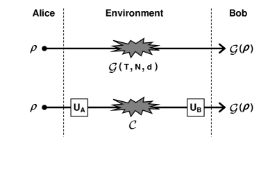
Figure 1: Reduction of a one-mode Gaussian channel $\mathcal{G}$ to its corresponding canonical form $\mathcal{C}$ by means of input-output Gaussian unitaries $\hat{U}_{A}$ and $\hat{U}_{B}$.

Depending on the values of the symplectic invariants $\det\mathbf{T}$, rank($\mathbf{T}$) and rank($\mathbf{N}$), we have six different expressions for the diagonal matrices $\mathbf{T}_{c},\mathbf{N}_{c}$ and, therefore, six inequivalent classes of canonical forms $\mathcal{C}=\mathcal{C}[\mathbf{T}_{c},\mathbf{N}_{c}]$, which are denoted by $A_{1},A_{2},B_{1},B_{2},C$ and $D$. From Ref. HolevoVittorio we report the classification of these forms in Table 1, where $\mathbf{Z}:=\mathrm{diag}(1,-1)$, $\mathbf{I}$ the identity matrix, and $\mathbf{0}$ the zero matrix. In this table $\tau:=\det\mathbf{T}$ is the (generalized) transmissivity, while $\bar{n}\geq 0$ is the thermal number of the environment and $\xi\geq 0$ is additive noise notation .

$$\tau:=\det\mathbf{T}$$ rk() rk() class

Table 1: Classification of canonical forms HolevoCanonical ; Caruso ; HolevoVittorio .

Let us also introduce the symplectic invariant

$$r:=\frac{\text{rank}(\mathbf{T})~{}\text{rank}(\mathbf{N})}{2}~{},$$ (22)

that we call the rank of the Gaussian channel formsREF ; RMP . Then, every class is simply determined by the pair $\{\tau,r\}$ according to the refined Table 2. Note that classes $B_{2}$ and $C$ have been divided into subclasses. In fact, class $B_{2}$ includes the identity channel (for $r=0$), while class $C$ describes an attenuator (amplifier) channel for $0<\tau<1$ ($\tau>1$). In common terminology the forms $A_{1}$, $B_{2}$ and $C$ are known as phase-insensitive, because they act symmetrically on the two input quadratures. By contrast, the forms $A_{2}$, $B_{1}$ and $D$ (conjugate of the amplifier) are all phase-sensitive. The form $B_{2}$ is an additive form. In fact it is also known as the additive-noise Gaussian channel, which is a direct generalization of the classical Gaussian channel in the quantum setting.

$$\tau$$ class sub

Id

Id

Att

Amp

      

Table 2: Refined classification of canonical forms.

II.3 Single-mode dilation of a canonical form

All the non-additive forms $\mathcal{C}[\tau,r,\bar{n}]$ admit a simple single-mode physical representation where the degrees of freedom $\hat{x}_{a}^{T}:=(\hat{q}_{a},\hat{p}_{a})$ of the input bosonic mode “$a$” unitarily interacts with the degrees of freedom $\hat{x}_{e}^{T}:=(\hat{q}_{e},\hat{p}_{e})$ of a single environmental bosonic mode “$e$” described by a mixed state $\rho_{e}$ Caruso ; HolevoVittorio  (see Fig. 2). In particular, such a physical representation can always be chosen to be Gaussian. This means that $\mathcal{C}[\tau,r,\bar{n}]$ can be represented by a canonical unitary $\hat{U}_{ae}$ mixing the input state $\rho_{a}$ with a thermal state $\rho_{e}(\bar{n})$, i.e.,

$$\mathcal{C}:\rho_{a}\rightarrow\mathcal{C}(\rho_{a})=\text{Tr}_{e}\left\{\hat{U}_{ae}\left[\rho_{a}\otimes\rho_{e}(\bar{n})\right]\hat{U}_{ae}^{\dagger}\right\},$$ (23)

where

$$\hat{U}_{ae}\left(\begin{array}[c]{c}\hat{x}_{a}\\ \hat{x}_{e}\end{array}\right)\hat{U}_{ae}^{\dagger}=\mathbf{M}\left(\begin{array}[c]{c}\hat{x}_{a}\\ \hat{x}_{e}\end{array}\right),$$ (24)

with $\mathbf{M}$ symplectic and $\rho_{e}(\bar{n})$ is a thermal state with CM $\mathbf{V}_{e}(\bar{n})=(2\bar{n}+1)\mathbf{I}$ (see Fig. 2).

In fact, by writing $\mathbf{M}$ in the blockform

$$\mathbf{M}=\left(\begin{array}[c]{cc}\mathbf{m}_{1}&\mathbf{m}_{2}\\ \mathbf{m}_{3}&\mathbf{m}_{4}\end{array}\right),$$ (25)

so that

$$\hat{x}_{a} \rightarrow\hat{x}_{b}:=\mathbf{m}_{1}\hat{x}_{a}+\mathbf{m}_{2}\hat{x}_{e}~{},$$ (26)

$$\hat{x}_{e} \rightarrow\hat{x}_{\tilde{e}}:=\mathbf{m}_{3}\hat{x}_{a}+\mathbf{m}_{4}\hat{x}_{e}~{},$$ (27)

one finds that Eq. (23) corresponds to the following input-output transformation for the characteristic function

$$\chi_{a}(\bm{\xi})\rightarrow\chi_{a}(\mathbf{m}_{1}^{T}\bm{\xi})\exp\left[-\tfrac{1}{2}(2\bar{n}+1)\left|\mathbf{m}_{2}^{T}\bm{\xi}\right|^{2}\right].$$ (28)

Then, by setting $\mathbf{m}_{1}^{T}=\mathbf{T}_{c}$ and

$$\mathbf{m}_{2}^{T}=\sqrt{\frac{\mathbf{N}_{c}}{2\bar{n}+1}}\mathbf{O},~{}~{}\mathbf{O}^{T}=\mathbf{O}^{-1},$$ (29)

one easily verifies that Eq. (28) has the form of Eq. (21), where the bona fide condition of Eq. (18) is assured by the symplectic nature of $\mathbf{M}$ NoteSympl . In Eq. (29) the orthogonal transformation $\mathbf{O}$ is chosen in a way to preserve the symplectic condition for $\mathbf{M}$. Such a condition also restricts the possible forms of the remaining blocks $\mathbf{m}_{3}$ and $\mathbf{m}_{4}$, which can be fixed up to a canonical local unitary.

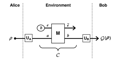
Figure 2: Single-mode physical representation of a non-additive canonical form $\mathcal{C}$ (all forms but $B_{2}$). This is also the physical representation of a non-additive Gaussian channel up to the input-output unitaries $\hat{U}_{A}$ and $\hat{U}_{B}$.

Altogether, any non-additive canonical form $\mathcal{C}[\tau,r,\bar{n}]$ can be described by a single-mode physical representation $\{\mathbf{M}(\tau,r),\rho_{e}(\bar{n})\}$ where the type of symplectic transformation $\mathbf{M}(\tau,r)$ is determined by its class $\{\tau,r\}$ while the thermal noise $\bar{n}$ only characterizes the environmental state. From the point of view of the second order statistical moments, the CM $\mathbf{V}_{a}$ of an input state $\rho_{a}$ undergoes the transformation

$$\mathbf{V}_{a}\rightarrow\mathrm{Tr}_{e}\left\{\mathbf{M}_{ae}(\tau,r)\left[\mathbf{V}_{a}\mathbf{\oplus}(2\bar{n}+1)\mathbf{I}_{e}\right]\mathbf{M}_{ae}(\tau,r)^{T}\right\},$$ (30)

where the partial trace $\mathrm{Tr}_{e}$ must be interpreted as deletion of rows and columns associated with mode $e$.

In particular, one has the following symplectic matrices for the various forms HolevoVittorio

$$\mathbf{M}(0<\tau<1,2)=\mathbf{M}(C)=\left(\begin{array}[c]{cc}\sqrt{\tau}\mathbf{I}&\sqrt{1-\tau}\mathbf{I}\\ -\sqrt{1-\tau}\mathbf{I}&\sqrt{\tau}\mathbf{I}\end{array}\right),$$ (31)

describing a beam-splitter,

$$\mathbf{M}(\tau>1,2)=\mathbf{M}(C)=\left(\begin{array}[c]{cc}\sqrt{\tau}\mathbf{I}&\sqrt{\tau-1}\mathbf{Z}\\ \sqrt{\tau-1}\mathbf{Z}&\sqrt{\tau}\mathbf{I}\end{array}\right),$$ (32)

describing an amplifier,

$$\mathbf{M}(\tau<0,2)=\mathbf{M}(D)=\left(\begin{array}[c]{cc}\sqrt{-\tau}\mathbf{Z}&\sqrt{1-\tau}\mathbf{I}\\ -\sqrt{1-\tau}\mathbf{I}&-\sqrt{-\tau}\mathbf{Z}\end{array}\right),$$ (33)

describing the complementary of an amplifier. Finally HolevoVittorio

$$\mathbf{M}(0,0) =\mathbf{M}(A_{1})=\left(\begin{array}[c]{cc}\mathbf{0}&\mathbf{I}\\ \mathbf{I}&\mathbf{0}\end{array}\right),$$ (36)

$$\mathbf{M}(0,1) =\mathbf{M}(A_{2})=\left(\begin{array}[c]{cc}\frac{\mathbf{I+Z}}{2}&\mathbf{I}\\ \mathbf{I}&\frac{\mathbf{Z-I}}{2}\end{array}\right),$$ (39)

$$\mathbf{M}(1,1) =\mathbf{M}(B_{1})=\left(\begin{array}[c]{cc}\mathbf{I}&\frac{\mathbf{I+Z}}{2}\\ \frac{\mathbf{I-Z}}{2}&\mathbf{-I}\end{array}\right).$$ (42)

II.4 Asymptotic dilation of the additive $B_{2}$ form

The additive-noise Gaussian channel or $B_{2}$ canonical form $\mathcal{C}[1,2,\xi]$ can be dilated into a two-mode environment HolevoVittorio . Another possibility is to describe this form by means of an asymptotic single-mode dilation. In fact, consider the dilation of the attenuator channel, which is a beam-splitter $\hat{U}_{ae}^{\text{BS}}(\tau)$ with transmissivity $\tau$ coupling the input mode $a$ with an environmental mode $e$ prepared in a thermal state $\rho_{e}(\bar{n})$ with $\bar{n}$ mean photons. In this dilation, let us consider a thermal state with $\bar{n}_{\xi,\tau}:=[\xi(1-\tau)^{-1}-1]/2$ so that we realize $(1-\tau)(2\bar{n}+1)=\xi$. Then, taking the limit for $\tau\rightarrow 1$ (so that $\bar{n}\rightarrow+\infty$), we represent the $B_{2}$ canonical form as

$$\mathcal{C}[1,2,\xi](\rho_{a})=\lim_{\tau\rightarrow 1}\text{Tr}_{e}\left\{\hat{U}_{ae}^{\text{BS}}(\tau)\left[\rho_{a}\otimes\rho_{e}(\bar{n}_{\xi,\tau})\right]\hat{U}_{ae}^{\text{BS}}(\tau)^{\dagger}\right\}.$$ (43)

In fact it is clear that, in this way, we may realize the asymptotic transformations $\mathbf{x}\rightarrow\mathbf{x}$ and $\mathbf{V}\longrightarrow\mathbf{V+}\xi\mathbf{I}$.

III Convergence of CV teleportation

III.1 Braunstein-Kimble teleportation protocol

Let us review the BK protocol for CV quantum teleportation Tele2 ; telereview . Alice and Bob share a resource state which is a two-mode squeezed vacuum (TMSV) state $\Phi_{AB}^{\mu}$. Recall that this is a zero-mean Gaussian state with CM RMP

$$\mathbf{V}^{\mu}=\left(\begin{array}[c]{cc}\mu\mathbf{I}&\sqrt{\mu^{2}-1}\mathbf{Z}\\ \sqrt{\mu^{2}-1}\mathbf{Z}&\mu\mathbf{I}\end{array}\right).$$ (44)

Here the variance parameter $\mu$ determines both the squeezing (or entanglement) and the energy associated with the state. In particular, we may write $\mu=2\bar{n}+1$, where $\bar{n}$ is the mean number of photons in each mode, $A$ (for Alice) and $B$ (for Bob).

Then, Alice has an input bipartite state $\rho_{Ra}$, where $R$ is an arbitrary multimode system while $a$ is a single mode that she wants to teleport to Bob. To teleport, she combines modes $a$ and $A$ in a joint CV Bell detection, whose complex outcome $\alpha$ is classically communicated to Bob (this can be realized by a balanced beam splitter followed by two conjugate homodyne detectors telereview ). Finally, Bob applies a displacement $D(-\alpha)$ on his mode $B$, so that the output state $\rho_{RB}$ is the teleported version $\rho_{Ra}^{\mu}$ of the input $\rho_{Ra}$.

One has perfect teleportation in the limit of infinite squeezing $\mu$. In other words, for any input state $\rho_{Ra}$ (with finite energy) we may write the trace norm limit

$$\lim_{\mu\rightarrow\infty}\left\|\rho_{Ra}^{\mu}-\rho_{Ra}\right\|=0,$$ (45)

or equivalently, we may write

$$\lim_{\mu\rightarrow\infty}F(\rho_{Ra}^{\mu},\rho_{Ra})=1,$$ (46)

where $F(\rho,\sigma):=\mathrm{Tr}\sqrt{\sqrt{\sigma}\rho\sqrt{\sigma}}$ is the Bures fidelity. This is a well known result which has been proven in Ref. Tele2 .

III.2 Strong convergence of CV teleportation

Let us denote by $\mathcal{T}$ the overall LOCC associated with the BK protocol, as in  Fig. 3(a). The application of this LOCC onto a finite-energy TMSV state $\Phi^{\mu}$ generates a teleportation channel $\mathcal{I}^{\mu}$ which is not the bosonic identity channel $\mathcal{I}$ but a point-wise (local) approximation of $\mathcal{I}$. In other words, for any (energy-bounded) input state $\rho_{Ra}$, we may consider the output

$$\rho_{Ra}^{\mu}:=\mathcal{I}_{R}\otimes\mathcal{I}_{a}^{\mu}(\rho_{Ra})=\mathcal{I}_{R}\otimes\mathcal{T}_{aAB}(\rho_{Ra}\otimes\Phi_{AB}^{\mu}),$$ (47)

and write the trace-norm limit

$$\lim_{\mu\rightarrow\infty}\left\|\mathcal{I}_{R}\otimes\mathcal{I}_{a}^{\mu}(\rho_{Ra})-\rho_{Ra}\right\|=0.$$ (48)

It is clear that this point-wise limit immediately implies the convergence in the strong topology Tele2

$$\sup_{\rho_{Ra}}\lim_{\mu\rightarrow\infty}\left\|\mathcal{I}_{R}\otimes\mathcal{I}_{a}^{\mu}(\rho_{Ra})-\rho_{Ra}\right\|=0.$$ (49)

Similarly, we may introduce the Bures distance qfi1

$$d_{\text{B}}(\rho,\sigma):=\sqrt{2[1-F(\rho,\sigma)]},$$ (50)

and write the previous limit as

$$\sup_{\rho_{Ra}}\lim_{\mu\rightarrow\infty}d_{\text{B}}[\mathcal{I}_{R}\otimes\mathcal{I}_{a}^{\mu}(\rho_{Ra}),\rho_{Ra}]=0.$$ (51)

Figure 3: BK protocol and teleportation simulation of bosonic channels. (a) We depict the BK protocol, where Alice’s mode $a$ of a bipartite input state $\rho_{Ra}$ is teleported to Bob’s mode $B$. This is performed by detecting mode $a$ along with mode $A$ of a TMSV state $\Phi^{\mu}$ via a Bell measurement. The complex output $\alpha$ is then used to apply the conditional displacement $D(-\alpha)$ on mode $B$. The output state $\rho_{RB}$ is an approximate version $\rho_{Ra}^{\mu}$ of the input state $\rho_{Ra}$. This output can be written as in Eq. (47) where $\mathcal{I}^{\mu}$ is the BK channel and $\mathcal{T}_{aAB}$ is the overall teleportation LOCC (Bell detection plus conditional displacements). (b) Consider a bosonic channel $\mathcal{E}$ applied to the output mode $B$, so that we may define the composite channel $\mathcal{E}^{\mu}=\mathcal{E}\circ\mathcal{I}^{\mu}$ as in Eq. (68). (c) If $\mathcal{E}$ is teleportation-covariant, we may write its teleportation simulation $\mathcal{E}^{\mu}$ as in Eq. (71) where the modified teleportation LOCC $\mathcal{\tilde{T}}$ (Bell detection and unitary corrections $V_{\alpha}$) is applied to the input and the quasi-Choi state $\rho_{\mathcal{E}}^{\mu}:=\mathcal{I}\otimes\mathcal{E}(\Phi^{\mu})$.

Remark 1

Let us stress that the strong convergence of the BK protocol is known since 1998. It is well-known that, for any given energy-constrained input state, if we send the squeezing of the resource state (TMSV state) to infinite, then we can perfectly teleport the input state. In Eqs. (4) and (8) of Ref. Tele2 , there is a convolution between the Wigner function $W_{\text{in}}$ of an arbitrary normalized input state and the Gaussian kernel $G_{\sigma}$, where $\sigma$ goes to zero for increasing squeezing $r$ (and ideal homodyne detectors). Taking the limit for large $r$, the teleportation fidelity goes to $1$ as we can also see from Eq. (11) of Ref. Tele2 . This is just a standard delta-like limit that does not really need explicit steps to be shown and fully provides the (strong) convergence of the BK protocol.

III.3 Bounded-uniform convergence of CV teleportation

Consider an energy-constrained alphabet of states

$$\mathcal{D}_{N}:=\{\rho_{Ra}~{}|~{}\mathrm{Tr}(\hat{N}\rho_{Ra})\leq N\},$$ (52)

where $\hat{N}$ is the total number operator associated with the input mode $a$ and the reference modes $R$. Then, we define an energy-constrained diamond distance PLOB ; TQC between two arbitrary bosonic channels $\mathcal{E}$ and $\mathcal{E}^{\prime}$, as

$$\left\|\mathcal{E}-\mathcal{E}^{\prime}\right\|_{\diamond N}:=\sup_{\rho_{Ra}\in\mathcal{D}_{N}}\left\|\mathcal{I}_{R}\otimes\mathcal{E}_{a}(\rho_{Ra})-\mathcal{I}_{R}\otimes\mathcal{E}_{a}^{\prime}(\rho_{Ra})\right\|~{}.$$ (53)

See also Ref. MaximNORM ; WinterNORM  for an alternate definition of energy-constrained diamond norm. It is easy to show that, for any finite energy $N$, one may write PLOB

$$\lim_{\mu\rightarrow\infty}\left\|\mathcal{I}^{\mu}-\mathcal{I}\right\|_{\diamond N}=0,$$ (54)

so that the BK channel $\mathcal{I}^{\mu}$ converges to the identity channel in the bounded-uniform topology. In fact, this comes from the point-wise limit in Eq. (48) combined with the fact that $\mathcal{D}_{N}$ is a compact set HolevoCOMPACT ; HolBook ; Werner .

III.4 Non-uniform convergence of CV teleportation

Can we relax the energy constraint $N$ in Eq. (54)? The answer is no. As already discussed in Ref. TQC , we have

$$\lim_{\mu\rightarrow\infty}\left\|\mathcal{I}^{\mu}-\mathcal{I}\right\|_{\diamond}=2,$$ (55)

where

$$\left\|\mathcal{E}-\mathcal{E}^{\prime}\right\|_{\diamond} =\lim_{N\rightarrow\infty}\left\|\mathcal{E}-\mathcal{E}^{\prime}\right\|_{\diamond N}$$ (56)

$$=\sup_{\rho_{Ra}}\left\|\mathcal{I}_{R}\otimes\mathcal{E}_{a}(\rho_{Ra})-\mathcal{I}_{R}\otimes\mathcal{E}_{a}^{\prime}(\rho_{Ra})\right\|$$ (57)

is the standard diamond distance. In fact, Ref. TQC provided a simple proof that the BK protocol does not uniformly converge to the identity channel. For this proof, it is sufficient to take the input state to be a TMSV state $\Phi^{\tilde{\mu}}$ with diverging energy $\tilde{\mu}$. Then, Eq. (55) is implied by the fact that, for any $\mu$-energy BK protocol, we have

$$\lim_{\tilde{\mu}\rightarrow\infty}\left\|\mathcal{I}_{R}\otimes\mathcal{I}_{a}^{\mu}(\Phi_{Ra}^{\tilde{\mu}})-\Phi_{Ra}^{\tilde{\mu}}\right\|=2,$$ (58)

which is equivalent to $\left\|\mathcal{I}^{\mu}-\mathcal{I}\right\|_{\diamond}=2$ for any $\mu$.

In order to show Eq. (58) we directly report the steps given in Ref. TQC but adapted to our different notation. The first observation is that, when applied to an energy-constrained quantum state (i.e., a “point”), the $\mu$-energy BK channel $\mathcal{I}^{\mu}$ is locally equivalent to an additive-noise Gaussian channel (form $B_{2}$) with added noise

$$\xi=2[\mu-\sqrt{\mu^{2}-1}]~{}.$$ (59)

For instance, see Refs. GerLimited ; next3 . Then, from the CM $\mathbf{V}^{\tilde{\mu}}$ of $\Phi_{Ra}^{\tilde{\mu}}$, it is easy to compute the CM of the output state $\rho_{Ra}^{\mu,\tilde{\mu}}:=\mathcal{I}_{R}\otimes\mathcal{I}_{a}^{\mu}(\Phi_{Ra}^{\tilde{\mu}})$ yielding

$$\mathbf{V}^{\mu,\tilde{\mu}}=\left(\begin{array}[c]{cc}\tilde{\mu}\mathbf{I}&\sqrt{\tilde{\mu}^{2}-1}\mathbf{Z}\\ \sqrt{\tilde{\mu}^{2}-1}\mathbf{Z}&(\tilde{\mu}+\xi)\mathbf{I}\end{array}\right).$$ (60)

Using the formula for the quantum fidelity between arbitrary Gaussian states banchiPRL2015 , we compute

$$F(\tilde{\mu},\mu):=F(\rho_{Ra}^{\mu,\tilde{\mu}},\Phi_{Ra}^{\tilde{\mu}})$$ (61)

$$=\frac{1}{\sqrt[4]{1-4\tilde{\mu}\left[\sqrt{4\mu^{2}-1}+\tilde{\mu}-2\mu(1+4\mu\tilde{\mu}-2\tilde{\mu}\sqrt{4\mu^{2}-1})\right]}}.$$

Here we notice the expansion $F(\tilde{\mu},\mu)\simeq O(\tilde{\mu}^{-1/2})$ at any fixed $\mu$. Now using the Fuchs-van de Graaf relations Fuchs

$$2[1-F(\rho,\sigma)]\leq\left\|\rho-\sigma\right\|\leq 2\sqrt{1-F(\rho,\sigma)^{2}},$$ (62)

we get, for any finite $\mu$, the following expansion

$$\left\|\rho_{Ra}^{\mu,\tilde{\mu}}-\Phi_{Ra}^{\tilde{\mu}}\right\|\geq 2-O(\tilde{\mu}^{-1/2}),$$ (63)

which implies Eq. (58).

Here it is important to observe the radically different behavior of the teleportation protocol with respect to exchanging the limits in the energy $\mu$ of the resource state $\Phi_{AB}^{\mu}$ and in the energy $\tilde{\mu}$ of the input state $\Phi_{Ra}^{\tilde{\mu}}$. In fact, by taking the limit in $\mu$ before the one in $\tilde{\mu}$ in Eq. (61), we get

$$F(\tilde{\mu},\mu)\simeq 1-O(\mu^{-1}).$$ (64)

Because of the non-commutation between these two limits

$$\lim_{\mu}\left[\lim_{\tilde{\mu}}F(\tilde{\mu},\mu)\right]\neq\lim_{\tilde{\mu}}\left[\lim_{\mu}F(\tilde{\mu},\mu)\right],$$ (65)

we have a difference between the strong convergence in Eq. (49) and the uniform non-convergence in Eq. (55). This also means that joint limits such as

$$\lim_{\mu,\tilde{\mu}}F(\tilde{\mu},\mu),~{}~{}~{}\underset{\mu,\tilde{\mu}}{\lim\sup}~{}F(\tilde{\mu},\mu)$$ (66)

are not defined. While this problem has been known since the early days of CV teleportation, technical errors related to this issue can still be found in recent literature (see the “case study” discussed in Sec. VII D).

IV Teleportation simulation of bosonic channels

The BK teleportation protocol is a fundamental tool for the simulation of bosonic channels (not necessarily Gaussian). Consider a teleportation-covariant bosonic channel $\mathcal{E}$ PLOB . This means that, for any random displacement $D(-\alpha)$, we may write

$$\mathcal{E}[D(-\alpha)\rho D(\alpha)]=V_{\alpha}\mathcal{E}(\rho)V_{\alpha}^{\dagger},$$ (67)

where $V_{\alpha}$ is an output unitary. If this is the case, then the bosonic channel $\mathcal{E}$ can be simulated by teleporting the input state with a modified teleportation LOCC $\mathcal{\tilde{T}}$ over the (asymptotic) Choi matrix $\rho_{\mathcal{E}}$ of the channel $\mathcal{E}$. In particular, Eq. (67) is true for Gaussian channels, for which $V_{\alpha}$ is just another displacement.

In order to correctly formulate this type of simulation, we need to start from an imperfect finite-energy simulation and then take the asymptotic limit for large energy. Therefore, let us consider a $\mu$-energy BK protocol $(\mathcal{T},\Phi^{\mu})$ generating a BK channel $\mathcal{I}^{\mu}$ at the input of a bosonic channel $\mathcal{E}$. Let us consider the composite channel

$$\mathcal{E}^{\mu}=\mathcal{E}\circ\mathcal{I}^{\mu}.$$ (68)

As shown in Fig. 3(b), for any input state $\rho_{Ra}$, we may write the output state as

$$\mathcal{I}_{R}\otimes\mathcal{E}_{a}^{\mu}(\rho_{Ra})=\mathcal{I}_{R}\otimes\mathcal{E}_{B}\circ\mathcal{T}_{aAB}(\rho_{Ra}\otimes\Phi_{AB}^{\mu}).$$ (69)

If the bosonic channel $\mathcal{E}$ is teleportation covariant, then we can swap it with the displacements $D(-\alpha)$, up to re-defining the teleportation corrections as $V_{\alpha}$. On the one hand this changes the teleportation LOCC $\mathcal{\tilde{T}}$, on the other hand the resource state becomes a quasi-Choi state

$$\rho_{\mathcal{E}}^{\mu}:=\mathcal{I}_{A}\circ\mathcal{E}_{B}(\Phi_{AB}^{\mu}).$$ (70)

Therefore, as depicted in Fig. 3(c), we may re-write the teleportation simulation of the output as

$$\mathcal{I}_{R}\otimes\mathcal{E}_{a}^{\mu}(\rho_{Ra})=\mathcal{I}_{R}\otimes\mathcal{\tilde{T}}_{aAB}\left[\rho_{Ra}\otimes(\rho_{\mathcal{E}}^{\mu})_{AB}\right].$$ (71)

Now, using Eq. (68) and the monotonicity of the trace distance under CPTP maps, we may write

$$\left\|\mathcal{I}_{R}\otimes\mathcal{E}_{a}^{\mu}(\rho_{Ra})-\mathcal{I}_{R}\otimes\mathcal{E}_{a}(\rho_{Ra})\right\|$$

$$=\left\|\mathcal{I}_{R}\otimes\mathcal{E}_{a}\circ\mathcal{I}_{a}^{\mu}(\rho_{Ra})-\mathcal{I}_{R}\otimes\mathcal{E}_{a}\circ\mathcal{I}_{a}(\rho_{Ra})\right\|$$

$$\leq\left\|\mathcal{I}_{R}\otimes\mathcal{I}_{a}^{\mu}(\rho_{Ra})-\rho_{Ra}\right\|\overset{\mu\rightarrow\infty}{\rightarrow}0,$$ (72)

where we exploit Eq. (48) in the last step. Therefore, for any bipartite (energy-constrained) input state $\rho_{Ra}$, we may write the point-wise limit

$$\lim_{\mu\rightarrow\infty}\left\|\mathcal{I}_{R}\otimes\mathcal{E}_{a}^{\mu}(\rho_{Ra})-\mathcal{I}_{R}\otimes\mathcal{E}_{a}(\rho_{Ra})\right\|=0.$$ (73)

IV.1 Strong convergence in the teleportation simulation of bosonic channels

The strong convergence in the simulation of (teleportation-covariant) bosonic channels (not necessarily Gaussian) is an immediate consequence of the point-wise limit in Eq. (73). In fact, because Eq. (73) holds for any bipartite (energy-constrained) input state $\rho_{Ra}$, we may write

$$\sup_{\rho_{Ra}}\lim_{\mu\rightarrow\infty}\left\|\mathcal{I}_{R}\otimes\mathcal{E}_{a}^{\mu}(\rho_{Ra})-\mathcal{I}_{R}\otimes\mathcal{E}_{a}(\rho_{Ra})\right\|=0,$$ (74)

or similarly in terms of the Bures distance

$$\sup_{\rho_{Ra}}\lim_{\mu\rightarrow\infty}d_{\text{B}}[\mathcal{I}_{R}\otimes\mathcal{E}_{a}^{\mu}(\rho_{Ra}),\mathcal{I}_{R}\otimes\mathcal{E}_{a}(\rho_{Ra})]=0.$$ (75)

In other words, the teleportation simulation $\mathcal{E}^{\mu}$ of a bosonic channel $\mathcal{E}$, strongly converges to it in the limit of large $\mu$.

IV.2 Bounded-uniform convergence in the teleportation simulation of bosonic channels

Consider now an energy constrained input alphabet $\mathcal{D}_{N}$ as in Eq. (52) and the energy-constrained diamond distance defined in Eq. (53). Given an arbitrary (teleportation-covariant) bosonic channel $\mathcal{E}$ and its teleportation simulation $\mathcal{E}^{\mu}$ as in Eq. (71), we define the simulation error as PLOB ; TQC

$$\delta(\mu,N):=\left\|\mathcal{E}^{\mu}-\mathcal{E}\right\|_{\diamond N}~{}.$$ (76)

Because of the monotonicity of the trace-distance under CPTP maps, we may certainly write

$$\delta(\mu,N) =\sup_{\rho_{Ra}\in\mathcal{D}_{N}}\left\|\mathcal{I}_{R}\otimes\mathcal{E}_{a}^{\mu}(\rho_{Ra})-\mathcal{I}_{R}\otimes\mathcal{E}_{a}(\rho_{Ra})\right\|$$ (77)

$$\leq\sup_{\rho_{Ra}\in\mathcal{D}_{N}}\left\|\mathcal{I}_{R}\otimes\mathcal{I}_{a}^{\mu}(\rho_{Ra})-\rho_{Ra}\right\|$$ (78)

$$:=\left\|\mathcal{I}^{\mu}-\mathcal{I}\right\|_{\diamond N}.$$ (79)

Therefore, from Eq. (54) we have that, for any finite energy $N$, we may write

$$\lim_{\mu\rightarrow\infty}\delta(\mu,N)=0.$$ (80)

In other words, for any (tele-covariant) bosonic channel $\mathcal{E}$, its teleportation simulation $\mathcal{E}^{\mu}$ converges to $\mathcal{E}$ in energy-bounded diamond norm. The question is: Can we remove the energy constraint? In the next section we completely characterize the condition that a bosonic Gaussian channel needs to satisfy in order to be simulated by teleportation according to the uniform topology (unconstrained diamond norm).

V Uniform convergence in the teleportation simulation of bosonic Gaussian channels

Let us now consider the convergence of the teleportation simulation in the uniform topology, i.e., according to the unconstrained diamond norm ($N\rightarrow\infty$). As we already know, this is a property that only certain bosonic channels may have. The simplest counter-example is certainly the identity channel for which the teleportation simulation via the BK protocol strongly but not uniformly converges. See Eqs. (49) and (55). As we will see below, this is also a problem for many Gaussian channels, including all the channels that can be represented as Gaussian unitaries, and those that can be reduced to the $B_{1}$ canonical form via unitary transformations. The theorem below establishes the exact condition that a single-mode Gaussian channel must have in order to be simulated by teleportation according to the uniform topology.

Theorem 2

Consider a single-mode bosonic Gaussian channel $\mathcal{G}[\mathbf{T},\mathbf{N},\mathbf{d}]$ and its teleportation simulation

$$\mathcal{G}^{\mu}(\rho)=\mathcal{\tilde{T}}_{aAB}\left[\rho_{a}\otimes(\rho_{\mathcal{G}}^{\mu})_{AB}\right],$$ (81)

where $\mathcal{\tilde{T}}_{aAB}$ is the LOCC  of a modified BK protocol implemented over the resource state$\ \rho_{\mathcal{G}}^{\mu}:=\mathcal{I}\otimes\mathcal{G}(\Phi^{\mu})$, with $\Phi^{\mu}$ being a TMSV state with energy $\mu$. Then, we have uniform convergence

$$\lim_{\mu\rightarrow\infty}\left\|\mathcal{G}^{\mu}-\mathcal{G}\right\|_{\diamond}=0,$$ (82)

if and only if the noise matrix $\mathbf{N}$ of the Gaussian channel $\mathcal{G}$ has full rank, i.e., $\mathrm{rank}(\mathbf{N})=2$.

Proof.  Let us start by showing the implication

$$\mathrm{rank}(\mathbf{N})=2\Longrightarrow\text{Eq.~{}(\ref{theo}).}$$ (83)

Consider an arbitrary single-mode Gaussian channel $\mathcal{G}[\mathbf{T},\mathbf{N},\mathbf{d}]$, so that it transforms the statistical moments as in Eq. (19). As we know from Eq. (69), for any input state $\rho_{Ra}$, we may write

$$\mathcal{I}_{R}\otimes\mathcal{G}^{\mu}(\rho_{Ra}) =\mathcal{I}_{R}\otimes\mathcal{G}_{B}\circ\mathcal{T}_{aAB}(\rho_{Ra}\otimes\Phi_{AB}^{\mu})$$ (84)

$$=\mathcal{I}_{R}\otimes(\mathcal{G}_{a}\circ\mathcal{I}_{a}^{\mu})(\rho_{Ra})$$ (85)

$$=\mathcal{I}_{R}\otimes\mathcal{G}_{a}^{\mu}(\rho_{Ra})$$ (86)

where $\mathcal{T}$ is the LOCC of the standard BK protocol and $\mathcal{I}^{\mu}$ is the BK channel, which is locally equivalent to an additive-noise Gaussian channel ($B_{2}$ form) with added noise $\xi$ as in Eq. (59). Therefore, for the Gaussian channel $\mathcal{G}^{\mu}$ we may write the modified transformations

$$\mathbf{\bar{x}\rightarrow\mathbf{T}\bar{x}}+\mathbf{d,}~{}~{}\mathbf{V}\rightarrow\mathbf{TVT}^{T}+\mathbf{N+}\xi\mathbf{TT}^{T}.$$ (87)

As we can see, the transformation of the first moments is identical. By contrast, the transformation of the second moments is characterized by the modified noise matrix

$$\mathbf{N}^{\xi}=\mathbf{N+}\xi\mathbf{TT}^{T}.$$ (88)

In order words, we may write $\mathcal{G}^{\mu}[\mathbf{\mathbf{T}},\mathbf{N}^{\xi},\mathbf{d}]$.

Because $\mathcal{G}$ and $\mathcal{G}^{\mu}$ have the same displacement, we can set $\mathbf{d}=\mathbf{0}$ without losing generality. Consider the unitary reduction of $\mathcal{G}[\mathbf{T},\mathbf{N},\mathbf{0}]$ into the corresponding canonical form $\mathcal{C}$ by means of two Gaussian unitaries $\hat{U}_{A}$ and $\hat{U}_{B}$ as in Eq. (20). Because $\mathbf{d}=\mathbf{0}$, we may assume that these unitaries are canonical (i.e., with zero displacement), so that they are one-to-one with two symplectic transformations, $\mathbf{S}_{A}$ and $\mathbf{S}_{B}$, in the phase space. To simplify the notation define the Gaussian channels

$$\mathcal{U}_{A}(\rho):=\hat{U}_{A}\rho\hat{U}_{A}^{\dagger},~{}\mathcal{U}_{B}(\rho):=\hat{U}_{B}\rho\hat{U}_{B}^{\dagger}.$$ (89)

Then we may write

$$\mathcal{G} =\mathcal{U}_{B}\circ\mathcal{C}\circ\mathcal{U}_{A},$$ (90)

$$\mathcal{G}^{\mu} =\mathcal{U}_{B}\circ\mathcal{C}\circ\mathcal{U}_{A}\circ\mathcal{I}^{\mu}.$$ (91)

Then notice that we may re-write

$$\mathcal{G}^{\mu}=\mathcal{U}_{B}\circ\mathcal{C}^{\mu}\circ\mathcal{U}_{A},$$ (92)

where we have defined

$$\mathcal{C}^{\mu}:=\mathcal{C}\circ\mathcal{U}_{A}\circ\mathcal{I}^{\mu}\circ\mathcal{U}_{A}^{-1}.$$ (93)

In Appendix A we prove the following.

Lemma 3

Consider a Gaussian channel $\mathcal{G}$ with $\tau:=\det\mathbf{T}\neq 1$ and $\mathrm{rank}(\mathbf{N})=2$. Then $\mathcal{C}$ and $\mathcal{C}^{\mu}$ have the same unitary dilation but different environmental states $\rho_{e}$ and $\rho_{e}^{\mu}$, i.e., for any input state $\rho$ we may write

$$\mathcal{C}(\rho)=\mathcal{D}(\rho\otimes\rho_{e}),~{}~{}\mathcal{C}^{\mu}(\rho)=\mathcal{D}(\rho\otimes\rho_{e}^{\mu}),$$ (94)

where $\mathcal{D}(\rho_{ae}):=\mathrm{Tr}_{e}\left(\hat{U}_{ae}\rho_{ae}\hat{U}_{ae}^{\dagger}\right)$ with $\hat{U}_{ae}$ unitary. Furthermore

$$\lim_{\mu\rightarrow\infty}F(\rho_{e}^{\mu},\rho_{e})=1.$$ (95)

Using this lemma in Eqs. (90) and (92) leads to

$$\mathcal{G}(\rho) =\mathcal{U}_{B}\circ\mathcal{D}[\mathcal{U}_{A}(\rho)\otimes\rho_{e}],$$ (96)

$$\mathcal{G}^{\mu}(\rho) =\mathcal{U}_{B}\circ\mathcal{D}[\mathcal{U}_{A}(\rho)\otimes\rho_{e}^{\mu}].$$ (97)

Clearly these relations can be extended to the presence of a reference system $R$, so that for any input $\rho_{Ra}$, we may write

$$\mathcal{I}_{R}\otimes\mathcal{G}_{a}(\rho_{Ra}) =\mathcal{I}_{R}\otimes\mathcal{U}_{B}\circ\mathcal{D}[\mathcal{U}_{A}(\rho_{Ra})\otimes\rho_{e}],$$ (98)

$$\mathcal{I}_{R}\otimes\mathcal{G}_{a}^{\mu}(\rho_{Ra}) =\mathcal{I}_{R}\otimes\mathcal{U}_{B}\circ\mathcal{D}[\mathcal{U}_{A}(\rho_{Ra})\otimes\rho_{e}^{\mu}].$$ (99)

As a result for any $\rho_{Ra}$, we may bound the trace distance as follows

$$\left\|\mathcal{I}_{R}\otimes\mathcal{G}_{a}^{\mu}(\rho_{Ra})-\mathcal{I}_{R}\otimes\mathcal{G}_{a}(\rho_{Ra})\right\|$$ (100)

$$=\left\|\mathcal{I}_{R}\otimes\mathcal{U}_{B}\circ\mathcal{D}[\mathcal{U}_{A}(\rho_{Ra})\otimes\rho_{e}^{\mu}]\right.$$

$$\left.-\mathcal{I}_{R}\otimes\mathcal{U}_{B}\circ\mathcal{D}[\mathcal{U}_{A}(\rho_{Ra})\otimes\rho_{e}]\right\|$$ (101)

$$\overset{(1)}{\leq}\left\|\mathcal{U}_{A}(\rho_{Ra})\otimes\rho_{e}^{\mu}-\mathcal{U}_{A}(\rho_{Ra})\otimes\rho_{e}\right\|$$ (102)

$$\overset{(2)}{=}\left\|\rho_{e}^{\mu}-\rho_{e}\right\|\overset{(3)}{\leq}2\sqrt{1-F(\rho_{e}^{\mu},\rho_{e})^{2}},$$ (103)

where we use: (1) the monotonicity under CPTP maps (including the partial trace) (2) multiplicity over tensor products; and (3) one of the Fuchs-van der Graaf relations. This is a very typical computation in teleportation stretching PLOB which has been adopted by several other authors in follow-up analyses.

As we can see the upper-bound in Eq. (103) does not depend on the input state $\rho_{Ra}$. Therefore, we may extend the result to the supremum and write

$$\left\|\mathcal{G}^{\mu}-\mathcal{G}\right\|_{\diamond} :=\sup_{\rho_{Ra}}\left\|\mathcal{I}_{R}\otimes\mathcal{G}_{a}^{\mu}(\rho_{Ra})-\mathcal{I}_{R}\otimes\mathcal{G}_{a}(\rho_{Ra})\right\|$$

$$\leq 2\sqrt{1-F(\rho_{e}^{\mu},\rho_{e})^{2}}.$$ (104)

Now, using Eq. (95), we obtain

$$\lim_{\mu\rightarrow\infty}\left\|\mathcal{G}^{\mu}-\mathcal{G}\right\|_{\diamond}=0,$$ (105)

proving the result for $\tau:=\det\mathbf{T}\neq 1$ and $\mathrm{rank}(\mathbf{N})=2$, i.e.,

$$\left.\begin{array}[c]{c}\tau:=\det\mathbf{T}\neq 1\\ \mathrm{rank}(\mathbf{N})=2{}{}{}\end{array}\right\}\Longrightarrow\text{Eq.~{}(\ref{theo}).}$$ (106)

Let us now remove the assumption $\tau:=\det\mathbf{T}\neq 1$. Note that the Gaussian channels with $\tau=1$ and $\mathrm{rank}(\mathbf{N})=2$ are those $\mathcal{\tilde{G}}$ unitarily equivalent to the $B_{2}$ form $\mathcal{C}[1,2,\xi^{\prime}]$ with added noise $\xi^{\prime}\geq 0$. In this case, we dilate the form in the asymptotic single-mode representation described in Sec. II.4. In other words, we may write

$$\mathcal{\tilde{G}} =\mathcal{U}_{B}\circ\mathcal{C}[1,2,\xi^{\prime}]\circ\mathcal{U}_{A}$$ (107)

$$=\mathcal{U}_{B}\circ\lim_{\tau\rightarrow 1}\mathcal{C}[\tau,2,\bar{n}_{\xi^{\prime},\tau}]\circ\mathcal{U}_{A}$$ (108)

$$=\lim_{\tau\rightarrow 1}~{}\mathcal{U}_{B}\circ\mathcal{C}[\tau,2,\bar{n}_{\xi^{\prime},\tau}]\circ\mathcal{U}_{A}$$ (109)

where $\bar{n}_{\xi^{\prime},\tau}:=[\xi^{\prime}(1-\tau)^{-1}-1]/2$ and it is easy to check the commutation of the limit. Let us call $\mathcal{B}_{\tau}$ the beam-splitter dilation associated with the attenuator $C$ form $\mathcal{C}[\tau,2,\bar{n}]$, and call $\rho_{e}(\bar{n})$ the corresponding thermal state of the environment. Then, we may write the approximation

$$\mathcal{\tilde{G}} =\lim_{\tau\rightarrow 1}~{}\mathcal{\tilde{G}}^{\tau},$$ (110)

$$\mathcal{\tilde{G}}^{\tau}(\rho) :=\mathcal{U}_{B}\circ\mathcal{B}_{\tau}[\mathcal{U}_{A}(\rho)\otimes\rho_{e}(\bar{n}_{\xi^{\prime},\tau})].$$ (111)

Similarly, for the teleportation-simulated channel, we may write

$$\mathcal{\tilde{G}}^{\mu} =\lim_{\tau\rightarrow 1}~{}\mathcal{\tilde{G}}^{\mu,\tau},$$ (112)

$$\mathcal{\tilde{G}}^{\mu,\tau}(\rho) :=\mathcal{U}_{B}\circ\mathcal{B}_{\tau}[\mathcal{U}_{A}(\rho)\otimes\rho_{e}^{\mu}(\bar{n}_{\xi^{\prime},\tau})],$$ (113)

where $\rho_{e}^{\mu}(\bar{n}_{\xi^{\prime},\tau})$ is a modified environmental state.

We can now exploit the triangle inequality. For any input $\rho$ and any $\tau<1$, we may write

$$\left\|\mathcal{\tilde{G}}^{\mu}(\rho)-\mathcal{\tilde{G}}(\rho)\right\| \leq\left\|\mathcal{\tilde{G}}^{\mu}(\rho)-\mathcal{\tilde{G}}^{\mu,\tau}(\rho)\right\|$$ (114)

$$+\left\|\mathcal{\tilde{G}}^{\mu,\tau}(\rho)-\mathcal{\tilde{G}}^{\tau}(\rho)\right\|+\left\|\mathcal{\tilde{G}}^{\tau}(\rho)-\mathcal{\tilde{G}}(\rho)\right\|.$$

By taking the limit for $\tau\rightarrow 1$ and using Eqs. (110) and (112), we find

$$\left\|\mathcal{\tilde{G}}^{\mu}(\rho)-\mathcal{\tilde{G}}(\rho)\right\|\leq\lim_{\tau\rightarrow 1}\left\|\mathcal{\tilde{G}}^{\mu,\tau}(\rho)-\mathcal{\tilde{G}}^{\tau}(\rho)\right\|~{}.$$ (115)

Repeating previous arguments, from Eqs. (111) and (113), we easily derive

$$\left\|\mathcal{\tilde{G}}^{\mu,\tau}(\rho)-\mathcal{\tilde{G}}^{\tau}(\rho)\right\|\leq 2\sqrt{1-F[\rho_{e}^{\mu}(\bar{n}_{\xi^{\prime},\tau}),\rho_{e}(\bar{n}_{\xi^{\prime},\tau})]^{2}},$$ (116)

so that

$$\left\|\mathcal{\tilde{G}}^{\mu}(\rho)-\mathcal{\tilde{G}}(\rho)\right\|\leq\lim_{\tau\rightarrow 1}~{}2\sqrt{1-F[\rho_{e}^{\mu}(\bar{n}_{\xi^{\prime},\tau}),\rho_{e}(\bar{n}_{\xi^{\prime},\tau})]^{2}}.$$ (117)

The previous inequality holds for any input state and can be easily extended to the presence of a reference system $R$, so that we may write

$$\left\|\mathcal{\tilde{G}}^{\mu}-\mathcal{\tilde{G}}\right\|_{\diamond}\leq\lim_{\tau\rightarrow 1}~{}2\sqrt{1-F[\rho_{e}^{\mu}(\bar{n}_{\xi^{\prime},\tau}),\rho_{e}(\bar{n}_{\xi^{\prime},\tau})]^{2}}.$$ (118)

One can easily check (see Appendix B), that the previous inequality leads to uniform convergence

$$\lim_{\mu\rightarrow\infty}\left\|\mathcal{\tilde{G}}^{\mu}-\mathcal{\tilde{G}}\right\|_{\diamond}=0~{},$$ (119)

completing the proof of the implication in Eq. (83).

Let us now show the opposite implication

$$\mathrm{rank}(\mathbf{N})=2\Longleftarrow\text{Eq.~{}(\ref{theo}),}$$ (120)

or, equivalently,

$$\mathrm{rank}(\mathbf{N})<2\Longrightarrow\text{No uniform convergence.}$$ (121)

Note that Gaussian channels with $\mathrm{rank}(\mathbf{N})<2$ are the identity channel $B_{2}(Id)$, having zero rank, and the $B_{1}$ form, having unit rank. We already know that there is no uniform convergence in the teleportation simulation of the identity channel and this property trivially extends to the teleportation simulation $\mathcal{U}^{\mu}=\mathcal{U}\circ\mathcal{I}^{\mu}$ of any Gaussian unitary $\mathcal{U}$. In fact, it is easy to check that

$$\left\|\mathcal{U}^{\mu}-\mathcal{U}\right\|_{\diamond}=\left\|\mathcal{I}^{\mu}-\mathcal{I}\right\|_{\diamond}=2~{},$$ (122)

due to invariance under unitaries. For the $B_{1}$ form $\mathcal{\tilde{C}}=\mathcal{C}[1,1,0]$, we now explicitly show that there is no uniform convergence in its teleportation simulation. Let us consider the simulation $\mathcal{\tilde{C}}^{\mu}$ by means of a $\mu$-energy BK protocol and consider an input TMSV state $\Phi_{Ra}^{\tilde{\mu}}$ with diverging energy $\tilde{\mu}$. We have the two output states

$$\rho_{Ra}^{\tilde{\mu}}:=\mathcal{I}_{R}\otimes\mathcal{\tilde{C}}_{a}(\Phi_{Ra}^{\tilde{\mu}}),~{}\rho_{Ra}^{\mu,\tilde{\mu}}:=\mathcal{I}_{R}\otimes\mathcal{\tilde{C}}_{a}^{\mu}(\Phi_{Ra}^{\tilde{\mu}}).$$ (123)

In particular, note that $\rho_{Ra}^{\mu,\tilde{\mu}}$ is a Gaussian state with CM

$$\mathbf{V}^{\mu,\tilde{\mu}}=\left(\begin{array}[c]{cccc}\tilde{\mu}&0&\sqrt{\tilde{\mu}^{2}-1}&0\\ 0&\tilde{\mu}&0&-\sqrt{\tilde{\mu}^{2}-1}\\ \sqrt{\tilde{\mu}^{2}-1}&0&\tilde{\mu}+\xi&0\\ 0&-\sqrt{\tilde{\mu}^{2}-1}&0&\tilde{\mu}+\xi+1\end{array}\right),$$ (124)

where $\xi$ is the added noise associated with the BK protocol and depends on $\mu$ according to Eq. (59). Using Eq. (62) we may write

$$\left\|\rho_{Ra}^{\mu,\tilde{\mu}}-\rho_{Ra}^{\tilde{\mu}}\right\|\geq 2\left[1-F\left(\rho_{Ra}^{\mu,\tilde{\mu}},\rho_{Ra}^{\tilde{\mu}}\right)\right].$$ (125)

Then, by computing the fidelity banchiPRL2015 and expanding in $\tilde{\mu}$, we obtain

$$F\left(\rho_{Ra}^{\mu,\tilde{\mu}},\rho_{Ra}^{\tilde{\mu}}\right)\simeq O(\tilde{\mu}^{-1/4}),$$ (126)

so that

$$\lim_{\tilde{\mu}\rightarrow\infty}\left\|\rho_{Ra}^{\mu,\tilde{\mu}}-\rho_{Ra}^{\tilde{\mu}}\right\|=2,$$ (127)

which clearly implies $\left\|\mathcal{\tilde{C}}^{\mu}-\mathcal{\tilde{C}}\right\|_{\diamond}=2$. Then, we may extend the result to any Gaussian channel which is unitarily equivalent to the $B_{1}$ form. Consider Eqs. (90) and (92) with $\mathcal{\tilde{C}}=\mathcal{C}[1,1,0]$, i.e,

$$\mathcal{G}=\mathcal{U}_{B}\circ\mathcal{\tilde{C}}\circ\mathcal{U}_{A},~{}~{}\mathcal{G}^{\mu}=\mathcal{U}_{B}\circ\mathcal{\tilde{C}}^{\mu}\circ\mathcal{U}_{A},$$ (128)

where

$$\mathcal{\tilde{C}}^{\mu}:=\mathcal{\tilde{C}}\circ\mathcal{U}_{A}\circ\mathcal{I}^{\mu}\circ\mathcal{U}_{A}^{-1}.$$ (129)

Assume the input state $\Psi_{Ra}^{\tilde{\mu}}:=\mathcal{I}_{R}\otimes\mathcal{U}_{A}^{-1}(\Phi_{Ra}^{\tilde{\mu}})$, so that we have the two output states

$$\rho_{Ra}^{\tilde{\mu}} :=\mathcal{I}_{R}\otimes\mathcal{G}_{a}(\Psi_{Ra}^{\tilde{\mu}})=\mathcal{I}_{R}\otimes\mathcal{U}_{B}\circ\mathcal{\tilde{C}}(\Phi_{Ra}^{\tilde{\mu}}),$$ (130)

$$\rho_{Ra}^{\mu,\tilde{\mu}} :=\mathcal{I}_{R}\otimes\mathcal{G}_{a}^{\mu}(\Psi_{Ra}^{\tilde{\mu}})=\mathcal{I}_{R}\otimes\mathcal{U}_{B}\circ\mathcal{\tilde{C}}^{\mu}(\Phi_{Ra}^{\tilde{\mu}}).$$ (131)

Because the fidelity is invariant under unitaries, we may neglect $\mathcal{U}_{B}$ and write

$$F\left(\rho_{Ra}^{\mu,\tilde{\mu}},\rho_{Ra}^{\tilde{\mu}}\right)=F\left[\mathcal{I}_{R}\otimes\mathcal{\tilde{C}}^{\mu}(\Phi_{Ra}^{\tilde{\mu}}),\mathcal{I}_{R}\otimes\mathcal{\tilde{C}}(\Phi_{Ra}^{\tilde{\mu}})\right].$$ (132)

Let us derive the CM $\mathbf{\tilde{V}}^{\mu,\tilde{\mu}}$ of the state $\mathcal{I}_{R}\otimes\mathcal{\tilde{C}}^{\mu}(\Phi_{Ra}^{\tilde{\mu}})$. Starting from the CM $\mathbf{V}^{\mu}$ of the TMSV in Eq. (44) and applying Eq. (129), we easily see that this CM is given by

$$\mathbf{\tilde{V}}^{\mu,\tilde{\mu}}=\mathbf{V}^{\mu}+\mathbf{0}\oplus\left[\xi\mathbf{S}_{A}\mathbf{S}_{A}^{T}+\text{{diag}}(0,1)\right],$$ (133)

where $\mathbf{0}$ is the $2\times 2$ zero matrix, and $\mathbf{S}_{A}$ is the symplectic matrix associated with the Gaussian unitary $\mathcal{U}_{A}$ (which can be taken to be canonical without losing generality). Let us set

$$\mathbf{S}_{A}=\left(\begin{array}[c]{cc}a&c\\ d&b\end{array}\right),$$ (134)

where the elements are real values such that $\det\mathbf{S}_{A}=+1$ (because $\mathbf{S}_{A}$ is symplectic). Then, we may compute the fidelity and expand it at the leading order in $\tilde{\mu}$, finding

$$F\left[\mathcal{I}_{R}\otimes\mathcal{\tilde{C}}^{\mu}(\Phi_{Ra}^{\tilde{\mu}}),\mathcal{I}_{R}\otimes\mathcal{\tilde{C}}(\Phi_{Ra}^{\tilde{\mu}})\right]^{4}$$

$$\simeq\gamma\tilde{\mu}^{-1}+O(\tilde{\mu}^{-3/2}),$$ (135)

$$\gamma :=\frac{a^{2}+c^{2}+2\xi}{2\xi(a^{2}+c^{2}+\xi)^{2}}>0.$$ (136)

Clearly, this implies $\left\|\mathcal{G}^{\mu}-\mathcal{G}\right\|_{\diamond}=2$ for any Gaussian channel unitarily equivalent to the $B_{1}$ form.$~{}\blacksquare$

Note that the rank of the noise matrix $\mathbf{N}$ is indeed a fundamental quantity in the previous proof. Given a single-mode Gaussian channel $\mathcal{G}[\mathbf{T},\mathbf{N},\mathbf{d}]$, consider its teleportation simulation $\mathcal{G}^{\mu}[\mathbf{\mathbf{T}},\mathbf{N}^{\xi},\mathbf{d}]$. For all channels with $\mathrm{rank}(\mathbf{N})=2$, we may write

$$\mathrm{rank}(\mathbf{N}^{\xi})=\mathrm{rank}(\mathbf{N})~{}~{}\text{for any }\xi\text{.}$$ (137)

This means that $\mathcal{G}^{\mu}$ may have the same canonical form and, therefore, the same unitary dilation as $\mathcal{G}$. By contrast, for Gaussian channels with $\mathrm{rank}(\mathbf{N})<2$, such as the identity channel or the $B_{1}$ form, we can see that we have $\mathrm{rank}(\mathbf{N}^{\xi})>\mathrm{rank}(\mathbf{N})$ for $\xi\neq 0$, so that the canonical form changes its class because of the teleportation simulation. As a result, the dilation changes and the data-processing bound in Eqs. (100)-(103) cannot be applied.

Remark 4

Our Theorem 2 straightforwardly solidifies all the claims of uniform convergence discussed in Ref. (WildePLAG, , v4) for very specific channels. Note that Ref. (WildePLAG, , v4) did not consider an arbitrary single-mode Gaussian channel, but only the canonical forms $C$ and $B_{2}$, without considering the action of input-output Gaussian unitaries. Furthermore, the other canonical forms, together with the Gaussian channels unitarily equivalent to them, were also not considered in Ref. (WildePLAG, , v4).

Remark 5

After our Theorem 2 was publicly available on the arXiv nostro , we noticed that Ref. WildePLAG was later updated into its $5^{th}$ version, where our key observation on the rank of the noise matrix of the Gaussian channel has been inserted (with no discussion of Ref. nostro ). In fact, see Theorem 6 in Ref. (WildePLAG, , v5) which appears to be an immediate extension of our Theorem 2.

VI Teleportation simulation of bosonic channels in adaptive protocols

We now discuss the teleportation simulation of bosonic channels within the context of adaptive protocols. This treatment is particularly important for its implications in quantum and private communications.

VI.1 Adaptive protocols

In an adaptive protocol, Alice and Bob, are connected by a quantum channel $\mathcal{E}$ at the ends of which they apply the most general quantum operations (QOs) allowed by quantum mechanics. If the task of the protocol is quantum channel discrimination or estimation, then Alice and Bob are the same entity ReviewMETRO ; PirCo . However, if the task of the protocol is quantum/private communication, Alice and Bob are distinct remote users and their QOs consist of local operations (LOs) assisted by unlimited and two-way classical communication (CC), briefly called adaptive LOCCs PLOB ; TQC . For simplicity, we consider here the second case only, i.e., communication.

The adaptive LOCCs are interleaved with the various transmissions through the channel. A compact formulation of the adaptive communication protocol goes as follows. Alice and Bob have local registers $\mathbf{a}$ and $\mathbf{b}$ prepared in some fundamental state $\rho_{\mathbf{a}}^{0}\otimes\rho_{\mathbf{b}}^{0}$. They apply a first adaptive LOCC $\Lambda_{0}$ so that $\rho_{\mathbf{ab}}^{0}=\Lambda_{0}(\rho_{\mathbf{a}}^{0}\otimes\rho_{\mathbf{b}}^{0})$. Then, Alice transmits one of her modes $a_{1}\in\mathbf{a}$ through the channel $\mathcal{E}$. Bob gets a corresponding output mode $b_{1}$ which is included in his register $b_{1}\mathbf{b}\rightarrow\mathbf{b}$. The two parties apply another adaptive LOCC $\Lambda_{1}$ to their updated registers, before the second transmission through the channel, and so on. After $n$ uses of the channel we have the output state

$$\rho_{\mathbf{ab}}^{n}=\Lambda_{n}\circ\mathcal{E}\circ\Lambda_{n-1}\cdots\circ\Lambda_{1}\circ\mathcal{E}\circ\Lambda_{0}(\rho_{\mathbf{a}}^{0}\otimes\rho_{\mathbf{b}}^{0}),$$ (138)

where we assume that channel $\mathcal{E}$ is applied to the input system $a_{i}$ in the $i$-th transmission, i.e., $\mathcal{E}=\mathcal{I}_{\mathbf{a}}\otimes\mathcal{E}_{a_{i}}\otimes\mathcal{I}_{\mathbf{b}}$.

Assume that Alice and Bob generate an output state $\rho_{\mathbf{ab}}^{n}$ which is epsilon-close to a private state KD $\phi_{n}$ with $nR_{n}$ secret bits, i.e., we have the trace-norm inequality

$$\left\|\rho_{\mathbf{ab}}^{n}-\phi_{n}\right\|\leq\varepsilon~{}.$$ (139)

Then, we say that the sequence $\mathcal{P}=\{\Lambda_{0},\ldots,\Lambda_{n}\}$ represents an $(n,\varepsilon,R_{n}^{\varepsilon})$ adaptive key generation protocol. By optimizing over all the protocols, we may write

$$K(\mathcal{E},n,\varepsilon)=\sup_{\mathcal{P}}R_{n}^{\varepsilon}~{}.$$ (140)

Taking the limit for large $n$ and small $\varepsilon$, one gets the secret key capacity of the channel $K(\mathcal{E})$.

VI.2 Simulation and “peeling” of adaptive protocols

Consider a tele-covariant bosonic channel $\mathcal{E}$. Then, let us assume a finite-energy BK protocol $(\mathcal{T},\Phi^{\mu})$ so that the bosonic channel $\mathcal{E}$ is approximated by its teleportation simulation $\mathcal{E}^{\mu}=\mathcal{E}\circ\mathcal{I}^{\mu}$, where $\mathcal{I}^{\mu}$ is the usual BK channel. In the adaptive protocol, we may then replace each instance of $\mathcal{E}$ with $\mathcal{E}^{\mu}$. This leads to a simulated protocol, with simulated output state $\rho_{\mathbf{ab}}^{\mu,n}$. A crucial step is to show how the error in the channel simulation $\mathcal{E}^{\mu}\simeq\mathcal{E}$ propagates to the output state $\rho_{\mathbf{ab}}^{\mu,n}\simeq\rho_{\mathbf{ab}}^{n}$ after $n$ uses of the adaptive protocol. This is done by adopting a peeling technique which suitably exploits data processing and the triangle inequality.

After $n$ uses of the simulated channel, we may write the output state as

$$\rho_{\mathbf{ab}}^{\mu,n}=\Lambda_{n}\circ\mathcal{E}^{\mu}\circ\Lambda_{n-1}\cdots\circ\Lambda_{1}\circ\mathcal{E}^{\mu}\circ\Lambda_{0}(\rho_{\mathbf{a}}^{0}\otimes\rho_{\mathbf{b}}^{0}),$$ (141)

where we assume that channel $\mathcal{E}^{\mu}$ is applied to the input system $a_{i}$ in the $i$-th transmission, i.e., $\mathcal{E}^{\mu}=\mathcal{I}_{\mathbf{a}}\otimes\mathcal{E}_{a_{i}}^{\mu}\otimes\mathcal{I}_{\mathbf{b}}$. We now want to evaluate the trace distance $\left\|\rho_{\mathbf{ab}}^{\mu,n}-\rho_{\mathbf{ab}}^{n}\right\|$ and show that this can be suitably bounded for any $n$. Let us start with the most elegant and rigorous approach, which has been discussed in Ref. TQC and directly comes from techniques in PLOB PLOB .

VI.2.1 Peeling in the bounded-uniform topology

The most rigorous way to show the peeling procedure is by using the energy-constrained diamond distance defined in Eq. (53) for an arbitrary but finite energy constraint $N$. As we have already written in Eq. (76), given an input alphabet $\mathcal{D}_{N}$ with maximum energy $N$, the simulation error between a bosonic channel $\mathcal{E}$ and its simulation $\mathcal{E}^{\mu}$ via the $\mu$-energy Braunstein-Kimble protocol can be written as PLOB ; TQC

$$\delta(\mu,N):=\left\|\mathcal{E}^{\mu}-\mathcal{E}\right\|_{\diamond N}\leq\left\|\mathcal{I}^{\mu}-\mathcal{I}\right\|_{\diamond N}~{}.$$ (142)

For any finite value of the constraint $N$, we may take the limit in $\mu\rightarrow\infty$ and write $\delta(\mu,N)\rightarrow 0$, thanks to the bounded-uniform convergence $\left\|\mathcal{I}^{\mu}-\mathcal{I}\right\|_{\diamond N}\overset{\mu\rightarrow\infty}{\rightarrow}0$.

Let us now express the output error $\left\|\rho_{\mathbf{ab}}^{\mu,n}-\rho_{\mathbf{ab}}^{n}\right\|$ in terms of the channel error $\delta(\mu,N)$. For simplicity, let us start by assuming $n=2$. From Eqs. (138) and (141) we may then write the peeling as PLOB

$$\|\rho_{\mathbf{ab}}^{\mu,2}-\rho_{\mathbf{ab}}^{2}\|$$

$$\overset{(1)}{\leq}\|\mathcal{E}^{\mu}\circ\Lambda_{1}\circ\mathcal{E}^{\mu}(\rho_{\mathbf{ab}}^{0})-\mathcal{E}\circ\Lambda_{1}\circ\mathcal{E}(\rho_{\mathbf{ab}}^{0})\|$$ (143)

$$\overset{(2)}{\leq}\|\mathcal{E}^{\mu}\circ\Lambda_{1}\circ\mathcal{E}^{\mu}(\rho_{\mathbf{ab}}^{0})-\mathcal{E}\circ\Lambda_{1}\circ\mathcal{E}^{\mu}(\rho_{\mathbf{ab}}^{0})\|$$

$$+\|\mathcal{E}\circ\Lambda_{1}\circ\mathcal{E}^{\mu}(\rho_{\mathbf{ab}}^{0})-\mathcal{E}\circ\Lambda_{1}\circ\mathcal{E}(\rho_{\mathbf{ab}}^{0})\|$$ (144)

$$\overset{(1)}{\leq}\|\mathcal{E}^{\mu}(\rho_{\mathbf{ab}}^{0})-\mathcal{E}(\rho_{\mathbf{ab}}^{0})\|$$

$$+\|\mathcal{E}^{\mu}[\Lambda_{1}\circ\mathcal{E}^{\mu}(\rho_{\mathbf{ab}}^{0})]-\mathcal{E}[\Lambda_{1}\circ\mathcal{E}^{\mu}(\rho_{\mathbf{ab}}^{0})]\|$$ (145)

$$\overset{(3)}{\leq}2\|\mathcal{E}^{\mu}-\mathcal{E}\|_{\Diamond N}=2\delta(\mu,N),$$ (146)

where we use: (1) The monotonicity of the trace distance under CPTP maps; (2) the triangle inequality; and (3) the energy-constrained diamond distance. Generalization to $n\geq 2$ gives the desired result

$$\left\|\rho_{\mathbf{ab}}^{\mu,n}-\rho_{\mathbf{ab}}^{n}\right\|\leq n\delta(\mu,N).$$ (147)

Now, for any finite $N$, we may take the limit for large $\mu$ and write

$$\left\|\rho_{\mathbf{ab}}^{\mu,n}-\rho_{\mathbf{ab}}^{n}\right\|\rightarrow 0.$$ (148)

VI.2.2 Peeling in the uniform topology

Consider an adaptive protocol over a bosonic Gaussian channel $\mathcal{G}[\mathbf{T},\mathbf{N},\mathbf{d}]$ with $\mathrm{rank}(N)=2$. In this case, we now know that we can remove the energy constraint in the diamond distance and write the following uniform convergence result

$$\left\|\mathcal{G}^{\mu}-\mathcal{G}\right\|_{\diamond}\overset{\mu\rightarrow\infty}{\rightarrow}0~{},$$ (149)

where $\mathcal{G}^{\mu}$ is the teleportation simulation of $\mathcal{G}$. It is clear that we can repeat the peeling and write

$$\left\|\rho_{\mathbf{ab}}^{\mu,n}-\rho_{\mathbf{ab}}^{n}\right\|\leq n\left\|\mathcal{G}^{\mu}-\mathcal{G}\right\|_{\diamond}\overset{\mu\rightarrow\infty}{\rightarrow}0.$$ (150)

VI.2.3 Peeling in the strong topology

The procedure can be trivially modified for strong convergence. In fact, starting from Eq. (145) we may write

$$\|\rho_{\mathbf{ab}}^{\mu,2}-\rho_{\mathbf{ab}}^{2}\|$$

$$\leq\|\mathcal{E}^{\mu}(\rho_{\mathbf{ab}}^{0})-\mathcal{E}(\rho_{\mathbf{ab}}^{0})\|$$

$$+\|\mathcal{E}^{\mu}[\Lambda_{1}\circ\mathcal{E}^{\mu}(\rho_{\mathbf{ab}}^{0})]-\mathcal{E}[\Lambda_{1}\circ\mathcal{E}^{\mu}(\rho_{\mathbf{ab}}^{0})]\|$$ (151)

$$=\|\mathcal{E}^{\mu}(\rho_{\mathbf{ab}}^{0})-\mathcal{E}(\rho_{\mathbf{ab}}^{0})\|+\|\mathcal{E}^{\mu}(\rho_{\mathbf{ab}}^{\mu,1})-\mathcal{E}(\rho_{\mathbf{ab}}^{\mu,1})\|,$$ (152)

where $\rho_{\mathbf{ab}}^{\mu,1}:=\Lambda_{1}\circ\mathcal{E}^{\mu}(\rho_{\mathbf{ab}}^{0})$ is an energy-constrained state. Then, we may write

$$\|\rho_{\mathbf{ab}}^{\mu,2}-\rho_{\mathbf{ab}}^{2}\|\leq 2\sup_{\rho_{\mathbf{ab}}}\|\mathcal{E}^{\mu}(\rho_{\mathbf{ab}})-\mathcal{E}(\rho_{\mathbf{ab}})\|.$$ (153)

Similarly, for $n$ uses, one derives

$$\|\rho_{\mathbf{ab}}^{\mu,n}-\rho_{\mathbf{ab}}^{n}\|\leq n\sup_{\rho_{\mathbf{ab}}}\|\mathcal{E}^{\mu}(\rho_{\mathbf{ab}})-\mathcal{E}(\rho_{\mathbf{ab}})\|.$$ (154)

Now using the strong convergence of the BK protocol, one gets

$$\|\rho_{\mathbf{ab}}^{\mu,n}-\rho_{\mathbf{ab}}^{n}\|\overset{\mu\rightarrow\infty}{\rightarrow}0.$$ (155)

This type of peeling is a trivial modification of the one presented in Sec. VI.2.1 and already adopted in PLOB and Ref. TQC .

Remark 6

Contrary to what claimed in the various arXiv versions of Ref. (WildePLAG, , v1-v5), none of the peeling techniques presented in this section can actually be found in WTB WildeFollowup . Therefore, the arguments presented in Ref. (WildePLAG, , v1-v5) are, as a matter of fact, a direct confirmation of the technical gaps and issues of WTB WildeFollowup .

VII Implications for quantum and private communications

Here we discuss how the previous notions can be used to rigorously prove the claims presented in WTB on the strong converse bounds for private communication over Gaussian channels. In order to clarify the technical problems, we first provide some preliminary notions, starting from the weak converse bounds established in PLOB and how the follow-up WTB attempted to show their strong converse property. Then, we discuss the basic technical errors in WTB and how these can be fixed by adopting a rigorous treatment of the BK protocol in adaptive protocols. Our proofs expand the very first one provided in Ref. TQC and based on the bounded-uniform convergence of the BK protocol.

VII.1 Background

Quantum and private communications over optical channels are inevitably limited by the presence of loss. In fact, the maximum number of secret bits that can be distributed over an optical fiber or a free-space link cannot be arbitrary but scales as $\simeq\tau$, where $\tau$ is the transmissivity of the communication channel. This is a fundamental rate-loss law that has attracted a lot of attention in the past years Rev1 ; Rev2 ; TGW ; PLOB . In 2009, Pirandola-Patrón-Braunstein-Lloyd Rev2 used the reverse coherent information Rev1 to compute the best-known achievable rate of $-\log_{2}(1-\tau)$ secret bits per use.

Later, in 2014, Takeoka-Guha-Wilde TGW computed the first upper bound $\log_{2}[(1+\tau)(1-\tau)]$ by resorting to the squashed entanglement Squash . Finally, in 2015, PLOB PLOB exploited quantum teleportation Tele1 ; Tele2 ; telereview and the relative entropy of entanglement REE1 ; REE2 ; REE3 to establish $-\log_{2}(1-\tau)$ as an upper bound, therefore discovering the secret-key capacity $K$ of the pure-loss channel. This result is also known as the PLOB bound. It was promptly generalized to repeater-assisted lossy communications netPAPER and its strong converse property was later investigated by WTB WildeFollowup .

In the bosonic setting, PLOB PLOB proved weak converse upper bounds for the private communication over single-mode phase-insensitive Gaussian channels RMP . In fact, let us introduce the entropic function

$$h(x):=(x+1)\log_{2}(x+1)-x\log_{2}x.$$ (156)

Then, for a thermal-loss channel $\mathcal{C}_{\tau,\bar{n}}^{\text{loss}}=\mathcal{C}[\tau,2,\bar{n}]$ with transmissivity $\tau\in[0,1]$ and mean thermal number $\bar{n}$ (canonical form $C$), one has PLOB

$$K(\mathcal{C}_{\tau,\bar{n}}^{\text{loss}}) \leq\Phi(\mathcal{C}_{\tau,\bar{n}}^{\text{loss}})$$ (157)

$$:=\left\{\begin{array}[c]{l}-\log_{2}\left[(1-\tau)\tau^{\bar{n}}\right]-h(\bar{n}),~{}~{}\text{for~{}}\bar{n}<\frac{\tau}{1-\tau},\\ 0\text{,~{}~{}otherwise.}\end{array}\right.$$ (160)

For a quantum amplifier $\mathcal{C}_{\tau,\bar{n}}^{\text{amp}}=\mathcal{C}[\tau,2,\bar{n}]$ with gain $\tau>1$ and mean thermal number $\bar{n}$ (canonical form $C$), one has the following bound PLOB

$$K(\mathcal{C}_{\tau,\bar{n}}^{\text{amp}}) \leq\Phi(\mathcal{C}_{\tau,\bar{n}}^{\text{amp}})$$ (161)

$$:=\left\{\begin{array}[c]{l}\log_{2}\left(\dfrac{\tau^{\bar{n}+1}}{\tau-1}\right)-h(\bar{n}),~{}~{}\text{for~{}}\bar{n}<(\tau-1)^{-1},\\ 0\text{,~{}~{}otherwise.}\end{array}\right.$$ (164)

Finally, for an additive-noise Gaussian channel $\mathcal{C}_{\xi}^{\text{add}}=\mathcal{C}[1,2,\xi]$ with added noise $\xi\geq 0$ (canonical form $B_{2}$), we may write PLOB

$$K(\mathcal{C}_{\xi}^{\text{add}})\leq\Phi(\mathcal{C}_{\xi}^{\text{add}}):=\left\{\begin{array}[c]{l}\frac{\xi-1}{\ln 2}-\log_{2}\xi,~{}~{}\text{for~{}}\xi<1,\\ 0\text{,~{}~{}otherwise.}\end{array}\right.$$ (165)

Remark 7

In a talk WildeQcrypt , an author wrongly claimed that the bounds in Eqs. (157), (161) and (165) would explode due to a technical issue related with the unboundedness of the “shield size” of the continuous-variable private state. This is not the case because the dimension of the private state was suitably truncated already in the first 2015 proof given by PLOB. See Ref. (TQC, , Sec. III) for further discussions and more details demystifying these claims.

Remark 8

As a direct result of his basic misunderstanding of the 2015 proof given by PLOB (see previous remark), the same author started to (unfairly) credit his follow-up work WTB WildeFollowup for the proof of the weak-converse upper bounds in Eqs. (157), (161) and (165). As one can easily check on the public arXiv, these bounds were fully established by PLOB in 2015, several months before WTB even made its first appearance (29 Feb 2016). From the chronology on the arXiv, one can also easily check that the main tools used in WTB were directly taken from PLOB. In this context, Ref. TQC fully clarifies how WTB is a direct follow-up work which is heavily based on results and tools in PLOB. This aspect is also very clear from the first arXiv version of WTB, where the presentation of previous results was sufficiently fair, but then its terminology was suddenly changed in its published version, where unfair claims have been made.

VII.2 General problems with the strong converse bounds claimed in WTB

Several months after the first version of PLOB, the follow-up paper WTB WildeFollowup also appeared on the arXiv. One of the main aims of WTB was to show that PLOB’s weak converse bounds for single-mode phase-insensitive bosonic Gaussian channels in Eqs. (157)-(165) also have the strong converse property. Recall that a weak converse bound means that perfect secret keys cannot be established at rates exceeding the bound. A strong converse bound is a refinement according to which even imperfect secret keys ($\varepsilon$-secure with $\varepsilon>0$) cannot be generated above the bound. In terms of methodology, WTB widely exploited the tools previously introduced by PLOB, in particular, the notion of a channel’s REE and the adaptive-to-block simplification via teleportation stretching. The combination of these two ingredients allowed PLOB (and later WTB) to write single-letter bounds in terms of the REE. However, differently from PLOB, WTB did not explicitly prove its statements for two main reasons:

(1)

WTB did not show how the error affecting the simulation of the bosonic channels is propagated to the output state of an adaptive protocol;

(2)

WTB did not show that such error converges to zero.

As a result of these two points, the bounds in WTB were not shown for adaptive protocols and, as presented there, they were technically equal to infinity. Let us describe these issues in details in the following section.

VII.3 Strong converse claims

In (WildeFollowup, , Theorem 24), WTB made the following claims on the strong-converse bound for single-mode phase-insensitive Gaussian channels.

WTB claims (WildeFollowup ). Consider an $\varepsilon$-secure key generation protocol over $n$ uses of a phase-insensitive canonical form $\mathcal{C}$, which may be a thermal-loss channel ($\mathcal{C}_{\tau,\bar{n}}^{\text{loss}}$), a quantum amplifier ($\mathcal{C}_{\tau,\bar{n}}^{\text{amp}}$) or an additive-noise Gaussian channel ($\mathcal{C}_{\xi}^{\text{add}}$). For any $\varepsilon\in(0,1)$ and $n\geq 1$, one may write the following upper bound for the secret key rate

$$K(\mathcal{C})\leq\Phi(\mathcal{C})+\sqrt{\frac{V(\mathcal{C})}{n(1-\varepsilon)}}+\frac{C(\varepsilon)}{n}~{},$$ (166)

where $\Phi(\mathcal{C})$ is PLOB’s weak converse bound given in Eqs. (157)-(165), $V(\mathcal{C})$ is a suitable “unconstrained relative entropy variance”, and

$$C(\varepsilon):=\log_{2}6+2\log_{2}\left(\frac{1+\varepsilon}{1-\varepsilon}\right).$$ (167)

In particular, for a pure loss channel ($\mathcal{C}_{\tau,0}^{\text{loss}}$) and a quantum-limited amplifier ($\mathcal{C}_{\tau,0}^{\text{amp}}$), one would have

$$K(\mathcal{C})\leq\Phi(\mathcal{C})+\frac{C(\varepsilon)}{n}~{}.$$ (168)

The above claims are obtained starting from a teleportation simulation based on the BK protocol with finite energy $\mu$ and then taking the limit of $\mu\rightarrow\infty$ (following PLOB). For any security parameter $\varepsilon\in(0,1)$, number of channel uses $n\geq 1$ and simulation energy $\mu$ with “infidelity” $\varepsilon_{\text{TP}}(n,\mu)$, one may write the following upper bound for the secret key rate of a phase insensitive canonical form $\mathcal{C}$

$$K(\mathcal{C})\leq\Phi(\mathcal{C})+\Delta(n,\mu).$$ (169)

At fixed $n$ and large $\mu$, $\Delta(n,\mu)$ has the expansion

$$\Delta(n,\mu)\simeq\sqrt{\frac{V(\mathcal{C})+O(\mu^{-1})}{n[1-\varepsilon(n,\mu)]}}+\frac{C[\varepsilon(n,\mu)]}{n}+O(\mu^{-1})~{},$$ (170)

where $\varepsilon(n,\mu)$ is an overall error defined as

$$\varepsilon(n,\mu):=\min\left\{1,\left[\sqrt{\varepsilon}+\sqrt{\varepsilon_{\text{TP}}(n,\mu)}\right]^{2}\right\},$$ (171)

where $\varepsilon_{\text{TP}}$ is associated with the teleportation simulation. For a pure loss channel ($\mathcal{C}_{\tau,0}^{\text{loss}}$) and a quantum-limited amplifier ($\mathcal{C}_{\tau,0}^{\text{amp}}$), one has Eq. (169), with

$$\Delta(n,\mu)\simeq n^{-1}C[\varepsilon(n,\mu)]+O(\mu^{-1}).$$ (172)

VII.4 Technical errors

In WTB the crucial technical error is clearly the treatment of the “infidelity” parameter $\varepsilon_{\text{TP}}$ which appears in Eq. (171) and is defined as the infidelity between the outputs of the protocol $\rho_{\mathbf{ab}}^{n}$ and the simulated protocol $\rho_{\mathbf{ab}}^{\mu,n}$ [in WTB denoted these as $\zeta_{AB}^{n}$ and $\zeta_{AB}^{\prime}(n,\mu)$]. More precisely, this is (WildeFollowup, , Eq. (177))

$$\varepsilon_{\text{TP}}(n,\mu):=1-F(\rho_{\mathbf{ab}}^{n},\rho_{\mathbf{ab}}^{\mu,n}),$$ (173)

where $F$ is the quantum fidelity. WTB argues that WildeFollowup

$$\begin{array}[c]{c}\text{\textquotedblleft{continuous variable\ teleportation}}\\ \text{{induces a perfect quantum channel}}\\ \text{{when infinite energy is available}\textquotedblright}\end{array}$$ (174)

which is the only reason why WTB states (WildeFollowup, , Eq. (178))

$$\underset{\mu\rightarrow\infty}{\lim\sup}~{}\varepsilon_{\text{TP}}(n,\mu)=0,~{}~{}\text{for any }n\text{.}$$ (175)

The first error is a basic misinterpretation of the convergence properties of the BK protocol. In fact, the statement (174) clearly means that the BK teleportation channel $\mathcal{I}^{\mu}$ generated by performing the protocol over a finite energy TMSV state $\Phi^{\mu}$ would reproduce the identity channel $\mathcal{I}$ (“perfect quantum channel”) when $\mu\rightarrow\infty$. We know that this is not true. In fact, as we have already shown in Eq. (55), we have

$$\lim_{\mu\rightarrow\infty}\left\|\mathcal{I}^{\mu}-\mathcal{I}\right\|_{\diamond}=2~{}.$$ (176)

In other words, the BK channel does not converge to the identity channel, as explained in detail in Sec. III.4 and already pointed out in Ref. TQC . Unfortunately, this has catastrophic consequences for the statement in Eq. (175) and all the WTB claims.

To make it simple, consider the single use ($n=1$) of a trivial adaptive protocol ($\Lambda_{1}=\mathcal{I}$) performed over channel $\mathcal{C}$ and its teleportation simulation $\mathcal{C}^{\mu}=\mathcal{C}\circ\mathcal{I}^{\mu}$. From Eqs. (138) and (141), we have the two output states

$$\rho_{\mathbf{ab}}^{1}=\mathcal{C}(\rho_{\mathbf{ab}}^{0}),~{}\rho_{\mathbf{ab}}^{\mu,1}=\mathcal{C}^{\mu}(\rho_{\mathbf{ab}}^{0}),$$ (177)

where the channels are meant to be applied to the input system $a_{1}$, i.e., $\mathcal{C}=\mathcal{I}_{\mathbf{a}}\otimes\mathcal{C}_{a_{1}}\otimes\mathcal{I}_{\mathbf{b}}$ and $\mathcal{C}^{\mu}=\mathcal{I}_{\mathbf{a}}\otimes\mathcal{C}_{a_{1}}^{\mu}\otimes\mathcal{I}_{\mathbf{b}}$. The infidelity is given by

$$\varepsilon_{\text{TP}}(1,\mu) =1-F(\rho_{\mathbf{ab}}^{1},\rho_{\mathbf{ab}}^{\mu,1})$$ (178)

$$=1-F[\mathcal{C}_{a_{1}}(\rho_{\mathbf{ab}}^{0}),\mathcal{C}_{a_{1}}^{\mu}(\rho_{\mathbf{ab}}^{0})]$$ (179)

$$\geq 1-F[\rho_{\mathbf{ab}}^{0},\mathcal{I}_{a_{1}}^{\mu}(\rho_{\mathbf{ab}}^{0})],$$ (180)

where we have exploited the monotonicity of the fidelity under CPTP maps, considering $\mathcal{C}=\mathcal{C}\circ\mathcal{I}$ and $\mathcal{C}^{\mu}=\mathcal{C}\circ\mathcal{I}^{\mu}$.

The proof idea in WTB was the exploitation of the (wrong) uniform limit $\mathcal{I}_{a_{1}}^{\mu}\overset{\mu}{\rightarrow}\mathcal{I}_{a_{1}}$ [see the statement in (174)], so that one could write $\lim_{\mu}F[\rho_{\mathbf{ab}}^{0},\mathcal{I}_{a_{1}}^{\mu}(\rho_{\mathbf{ab}}^{0})]=1$ in Eq. (180). Instead, assume that Alice is sending part of a TMSV state $\Phi^{\tilde{\mu}}$ with energy $\tilde{\mu}$. This means that we may decompose $\rho_{\mathbf{ab}}^{0}=\rho_{\mathbf{a}}^{0}\otimes\Phi_{aa_{1}}^{\tilde{\mu}}\otimes\rho_{\mathbf{b}}^{0}$, and write

$$\varepsilon_{\text{TP}}(1,\mu)\geq 1-F[\Phi_{aa_{1}}^{\tilde{\mu}},\mathcal{I}_{a}\otimes\mathcal{I}_{a_{1}}^{\mu}(\Phi_{aa_{1}}^{\tilde{\mu}})],$$ (181)

where we use the multiplicativity of the fidelity under tensor products. Taking the $\lim\sup_{\mu}$ of $\varepsilon_{\text{TP}}(1,\mu)$ means to include all the possible input states. Because the input alphabet is unbounded (as it should be when we consider unconstrained quantum and private capacities), this means that the alphabet also includes the limit of asymptotic states, such as $\Phi_{aa_{1}}^{\tilde{\mu}}$ for large $\tilde{\mu}$.

Also note that the generic limit in Eq. (175) does not imply any specific order of the limits between the simulation energy $\mu$ and the input energy $\tilde{\mu}$ of the alphabet. For an unbounded alphabet, we can equivalently interpret

$$\underset{\mu}{\lim\sup}=\lim_{\mu}\lim_{\tilde{\mu}}\text{~{}~{}OR~{}}~{}\underset{\mu}{\lim\sup}=\lim_{\tilde{\mu}}\lim_{\mu}~{}.$$ (182)

Therefore, if we apply the first case to Eq. (181) we find

$$\underset{\mu\rightarrow\infty}{\lim\sup~{}}\varepsilon_{\text{TP}}(1,\mu)$$

$$\geq 1-\lim_{\mu\rightarrow\infty}\lim_{\tilde{\mu}\rightarrow\infty}F[\Phi_{aa_{1}}^{\tilde{\mu}},\mathcal{I}_{a}\otimes\mathcal{I}_{a_{1}}^{\mu}(\Phi_{aa_{1}}^{\tilde{\mu}})]$$

$$\geq 1~{},$$ (183)

because, as we know, $F[\Phi_{aa_{1}}^{\tilde{\mu}},\mathcal{I}_{a}\otimes\mathcal{I}_{a_{1}}^{\mu}(\Phi_{aa_{1}}^{\tilde{\mu}})]\simeq O(\tilde{\mu}^{-1})$ at any fixed $\mu$. This result disproves the claim in Eq. (175) already for the trivial case of $n=1$.

Remark 9

It is important to remark that the ambiguity in Eq. (182) is not addressed, discussed or noted in any part of WTB, where the convergence problems of the BK protocol are just completely ignored. In WTB there is no discussion related to uniform convergence [associated with the first order of the limits in Eq. (182)] or strong convergence [associated with the second order of the limits in Eq. (182)]. Also note that the additional arguments presented in the various arXiv versions of Ref. (WildePLAG, , v1-v5) can be seen as an erratum de facto of WTB, rather than a justification of its proofs as claimed by the author.

As the “proof” has been carried out in WTB, one must conclude that

$$\underset{\mu\rightarrow\infty}{\lim\sup}~{}\varepsilon_{\text{TP}}(n,\mu)=1,~{}~{}\text{for any }n\text{,}$$ (184)

which is exactly the opposite of the claim in Eq. (175). In fact, one can extend the previous reasoning to any $n$ and any adaptive protocol (which is the content of the next section). The result in Eq. (184) implies $\lim\sup_{\mu}~{}\varepsilon(n,\mu)=1$ for the overall error in Eq. (171). Unfortunately, this leads to $C[\varepsilon(n,\mu)]\rightarrow\infty$ in Eq. (170) and, therefore, all the bounds claimed by WTB in Eq. (169) are divergent, i.e.,

$$K(\mathcal{C})\leq\Phi(\mathcal{C})+\infty~{}.$$ (185)

VII.5 Filling the technical gaps

It is important to note that, in WTB, the simulation error on the output state $\varepsilon_{\text{TP}}(n,\mu)$ is completely disconnected from the error on the channel simulation which affects each transmission. In other words, there are no rigorous relations such as those given in Eqs. (147), (150) or (154) for the various forms of convergence. The reason is because in WTB there is no peeling argument PLOB ; TQC which simplifies the adaptive protocol and relates the output error $\left\|\rho_{\mathbf{ab}}^{\mu,n}-\rho_{\mathbf{ab}}^{n}\right\|$ to the channel error $\mathcal{C}^{\mu}\neq\mathcal{C}$. As a result, the WTB claims not only are not proven (due to the divergences) but they do not even apply to adaptive protocols. Here we apply the peeling argument to correctly write $\varepsilon_{\text{TP}}(n,\mu)$ in the presence of an adaptive protocol. This extends the considerations already made in Ref. TQC for the bounded-uniform convergence to the other forms of convergence (strong and uniform).

Using the Fuchs-van der Graaf relations of Eq. (62), we may write

$$\varepsilon_{\text{TP}}(n,\mu)\leq\frac{\left\|\rho_{\mathbf{ab}}^{n}-\rho_{\mathbf{ab}}^{\mu,n}\right\|}{2}~{}.$$ (186)

Following PLOB and Ref. TQC , we may consider the energy-constrained diamond distance and perform the peeling procedure in Eqs. (143)-(146) which leads to the result in Eq. (147). Therefore, we may write

$$\varepsilon_{\text{TP}}(n,\mu)\leq n\delta(\mu,N)/2,$$ (187)

where $\delta(\mu,N):=\left\|\mathcal{C}^{\mu}-\mathcal{C}\right\|_{\diamond N}$. Once we have the control on the error, we may take the limit for large $\mu$. For any number of channel uses $n$ and finite energy constraint $N$, we may safely write

$$\underset{\mu\rightarrow\infty}{\lim\sup}~{}\varepsilon_{\text{TP}}(n,\mu|N)\leq\lim_{\mu\rightarrow\infty}~{}n\delta(\mu,N)/2=0~{},$$ (188)

proving Eq. (175) and the corresponding WTB claims.

More precisely, starting from Eq. (188), we may write the following upper bound for the energy-constrained key capacity TQC

$$K(\mathcal{C}|N)\leq\Phi(\mathcal{C})+\Delta(n,\mu|N)~{},$$ (189)

where $\Delta(n,\mu|N)$ is computed assuming the energy constraint. For large $\mu$, we may now write

$$\Delta(n,\mu|N)\rightarrow\sqrt{\frac{V(\mathcal{C})}{n(1-\varepsilon)}}+\frac{C(\varepsilon)}{n}.$$ (190)

Because $\lim_{\mu}\Delta(n,\mu|N)$ does not depend on $N$, we can extend the inequality in Eq. (189) to the supremum $K(\mathcal{C}):=\sup_{N}K(\mathcal{C}|N)$, so that

$$K(\mathcal{C})\leq\Phi(\mathcal{C})+\lim_{\mu\rightarrow\infty}\Delta(n,\mu|N),$$ (191)

proving the strong converse bound claimed in Eq. (166).

Additional proofs can be made assuming the other types of convergence (strong and uniform). These are simple variants of the previous one. First of all, because we consider phase-insensitive canonical forms, we now know that the teleportation simulation converges uniformly, i.e., $\left\|\mathcal{C}^{\mu}-\mathcal{C}\right\|_{\diamond}\overset{\mu\rightarrow\infty}{\rightarrow}0$. This means that we may directly consider $N=\infty$ in the previous proof, so that we can delete the conditioning from the energy constraint $N$ and the last step (supremum in $N)$ is not needed. Another approach is considering the strong convergence of the teleportation simulation. After the peeling procedure, this means that we may write Eq. (154), so that

$$\varepsilon_{\text{TP}}(n,\mu)\leq\frac{n}{2}\sup_{\rho_{\mathbf{ab}}}\|\mathcal{C}(\rho_{\mathbf{ab}})-\mathcal{C}^{\mu}(\rho_{\mathbf{ab}})\|\overset{\mu\rightarrow\infty}{\rightarrow}0.$$ (192)

Remark 10

It is easy to check that none of these techniques have been explicitly or even implicitly discussed in WTB, contrary to what claimed in the various arXiv versions of Ref. (WildePLAG, , v1-v5).

VIII Conclusions

In this work we have discussed the Braunstein-Kimble teleportation protocol for bosonic systems and its application to the simulation of bosonic channels. We have considered the various forms (topologies) of convergence of this protocol to the identity channel, which are still the subject of basic misunderstandings for some authors. As a completely new result, we have shown that the teleportation simulation of an arbitrary single-mode Gaussian channel (not necessarily in canonical form) uniformly converges to the channel in the limit of infinite energy, as long as the channel has a full rank noise matrix.

We have then discussed the various forms of convergence in the context of adaptive protocols, following the ideas established in PLOB PLOB . In this scenario, it is essential to provide a peeling procedure which relates the simulation error on the final output state to the simulation error affecting the individual channel transmissions. As an application, we exploit this peeling argument and the various convergence topologies to completely prove the claims presented in WTB in relation to private communication over bosonic Gaussian channels. This treatment extends the first rigorous proof given in Ref. TQC and specifically based on the bounded-uniform convergence (energy-constrained diamond distance).

Acknowledgments.  This research has been funded by the EPSRC via the ‘UK Quantum Communications HUB’ (Grant no. EP/M013472/1) and the Innovation Fund Denmark (Qubiz project). The authors would like to thank discussions with C. Ottaviani, T. P. W. Cope, G. Spedalieri, and L. Banchi.

Author contribution statement. The authors contributed equally to the manuscript.

Appendix A Proof of Lemma 3

Consider the canonical forms $\mathcal{C}$ with $\tau:=\det\mathbf{T}\neq 1$ and $\text{rank}(\mathbf{N})=2$. These correspond to $A_{2}$, $C($Att$)$, $C($Amp$)$, and $D$. Given $\mathcal{C}$, consider the variant

$$\mathcal{C}^{\mu}:=\mathcal{C}\circ\mathcal{U}_{A}\circ\mathcal{I}^{\mu}\circ\mathcal{U}_{A}^{-1},$$ (193)

where $\mathcal{U}_{A}$ is a canonical Gaussian unitary with associated symplectic matrix $\mathbf{S}_{A}$, and $\mathcal{I}^{\mu}$ is the BK teleportation channel, which is locally (point-wise) equivalent to an additive-noise Gaussian channel ($B_{2}$ form) with added noise

$$\xi=2[\mu-\sqrt{\mu^{2}-1}].$$ (194)

Note that we may use the Bloch-Messiah decomposition SamMessiah

$$\mathbf{S}_{A}=\mathbf{O}_{1}\mathbf{S}_{q}\mathbf{O}_{2},$$ (195)

where $\mathbf{O}$’s are symplectic orthogonal matrices, while $\mathbf{S}_{q}=\mathrm{diag}(r,r^{-1})$ for $r>0$ is a squeezing matrix Euler . Here we show that $\mathcal{C}$ and $\mathcal{C}^{\mu}$ have the same unitary dilation with different environmental states $\rho_{e}$ and $\rho_{e}^{\mu}$, whose fidelity $F(\rho_{e}^{\mu},\rho_{e})\overset{\mu\rightarrow\infty}{\rightarrow}1$. Let us start with the form $C$.

A.1 Lossy channel $C($Att$)$ and amplifier $C($Amp$)$

Consider the canonical $C$ form $\mathcal{C}(\tau>0,2,\bar{n})$ representing either a thermal-loss channel ($0<\tau<1$) or a noisy quantum amplifier ($\tau>1$). Their action on the input covariance matrix (CM) $\mathbf{V}$ is given by

$$\mathbf{V}\rightarrow\tau\mathbf{V}+|1-\tau|\omega\mathbf{I}~{},$$ (196)

where $\omega:=2\bar{n}+1\geq 1$. From Eq. (193), we may write

$$\mathbf{V} \rightarrow\tau(\mathbf{V}+\xi\mathbf{S}_{A}\mathbf{S}_{A}^{T})+|1-\tau|\omega\mathbf{I}$$

$$=\tau\mathbf{V}+|1-\tau|\mathbf{\tilde{W}},$$ (197)

where we have set

$$\mathbf{\tilde{W}}:=\omega\mathbf{I}+\gamma\mathbf{S}_{A}\mathbf{S}_{A}^{T},~{}~{}\gamma:=\frac{\xi\tau}{|1-\tau|}\geq 0.$$ (198)

According to Eqs. (197) and (198), we may represent $\mathcal{C}^{\mu}(\tau>0,2,\bar{n})$ with the same two-mode symplectic matrix $\mathbf{M}(C)$ of the original $C$ form, but replacing the thermal state $\rho_{e}(\bar{n})$ with a zero-mean Gaussian state $\rho_{e}^{\mu}$ whose CM can be written as $\mathbf{\tilde{W}}$. To check this is indeed the case, we need to verify that $\mathbf{\tilde{W}}$ is a bona fide CM  bonafide . It is certainly positive definite, so we just need to check that its symplectic eigenvalue is greater than $1$. Note that we may apply the orthogonal symplectic $\mathbf{O}_{1}$ so that

$$\mathbf{W:}=\mathbf{O}_{1}^{T}\mathbf{\tilde{W}O}_{1}=\omega\mathbf{I}+\gamma\mathbf{S}_{q}^{2}~{}.$$ (199)

The symplectic eigenvalue is equal to

$$\nu =\sqrt{\det\mathbf{W}}=\sqrt{\omega^{2}+\gamma^{2}+\gamma\omega\left(r^{2}+1/r^{2}\right)}$$

$$\geq\omega+\gamma\geq 1~{}.$$ (200)

Finally we compute the fidelity between the environmental states, finding

$$F(\rho_{e}^{\mu},\rho_{e})=\sqrt{2r}\left[\sqrt{\left(\gamma r^{2}\omega+\omega^{2}+1\right)\left(\gamma\omega+r^{2}\left(\omega^{2}+1\right)\right)}\right.$$

$$-\left.\sqrt{\left(\omega^{2}-1\right)\left(\gamma\omega+\gamma r^{4}\omega+r^{2}\left(\gamma^{2}+\omega^{2}-1\right)\right)}\right]^{-1/2},$$ (201)

which goes to $1$ for $\mu\rightarrow\infty$ (so that $\xi\rightarrow 0$ and $\gamma\rightarrow 0$). This is true for any finite value of the squeezing $r>0$ and the thermal variance $\omega$.

A.2 Conjugate of the amplifier $D$

Let us consider the $D$ form $\mathcal{C}(\tau<0,2,\bar{n})$ which transforms the input as follows

$$\mathbf{V}\rightarrow-\tau\mathbf{ZVZ}+(1-\tau)\omega\mathbf{I}.$$ (202)

Then, the action of $\mathcal{C}^{\mu}(\tau<0,2,\bar{n})$ can be written as

$$\mathbf{V} \rightarrow-\tau\mathbf{Z}(\mathbf{V}+\xi\mathbf{S}_{A}\mathbf{S}_{A}^{T})\mathbf{Z}+(1-\tau)\omega\mathbf{I}$$

$$=-\tau\mathbf{Z}\mathbf{V}\mathbf{Z}+(1-\tau)\left(\omega\mathbf{I}-\kappa\mathbf{Z}\mathbf{S}_{A}\mathbf{S}_{A}^{T}\mathbf{Z}\right)$$

$$=-\tau\mathbf{Z}\mathbf{V}\mathbf{Z}+(1-\tau)\mathbf{\tilde{W}}$$ (203)

where $\kappa:=\xi\tau/(1-\tau)\leq 0$. Using the Bloch-Messiah decomposition of Eq. (195) and $\mathbf{ZS}_{q}^{2}\mathbf{Z}=\mathbf{S}_{q}^{2}$, we may write

$$\mathbf{\tilde{W}} =\omega\mathbf{I}-\kappa\mathbf{ZO}_{1}\mathbf{S}_{q}^{2}\mathbf{O}_{1}^{T}\mathbf{Z}$$

$$=\omega\mathbf{I}-\kappa(\mathbf{ZO}_{1}\mathbf{Z)S}_{q}^{2}(\mathbf{ZO}_{1}^{T}\mathbf{Z).}$$ (204)

Thus, we may represent $\mathcal{C}^{\mu}(\tau<0,2,\bar{n})$ with the same two-mode symplectic matrix $\mathbf{M}(D)$ as the original $D$ form, but replacing the thermal state $\rho_{e}(\bar{n})$ with a zero-mean Gaussian state $\rho_{e}^{\mu}$ whose CM can be written as $\mathbf{\tilde{W}}$ in Eq. (204). To check this is indeed the case, we need to verify that $\mathbf{\tilde{W}}$ is a bona fide CM bonafide . First notice that the matrix $\bm{\Sigma}:=\mathbf{ZO}_{1}\mathbf{Z}$ is orthogonal and symplectic. We may therefore apply the symplectic $\bm{\Sigma}^{T}$ and write

$$\mathbf{W}=\bm{\Sigma}^{T}\mathbf{\tilde{W}}\bm{\Sigma}=\omega\mathbf{I}-\kappa\mathbf{S}_{q}^{2}~{}.$$

Because $\kappa\leq 0$, this is positive definite and it has symplectic eigenvalue

$$\nu =\sqrt{\omega^{2}+\kappa^{2}-\omega\kappa(r^{2}+1/r^{2})}$$

$$\geq\omega-\kappa\geq 1~{}.$$ (205)

Finally we compute the fidelity between the environmental states, finding

$$F(\rho_{e}^{\mu},\rho_{e})=\sqrt{2r}\left[\sqrt{\left(-\kappa r^{2}\omega+\omega^{2}+1\right)\left(-\kappa\omega+r^{2}\left(\omega^{2}+1\right)\right)}\right.$$

$$\left.-\sqrt{\left(1-\omega^{2}\right)\left(\kappa\omega+\kappa r^{4}\omega-r^{2}\left(\kappa^{2}+\omega^{2}-1\right)\right)}\right]^{-1/2},$$ (206)

which goes to $1$ for large $\mu$ (so that $\xi\rightarrow 0$ and $\kappa\rightarrow 0$). This is true for any finite value of the squeezing $r>0$ and the thermal variance $\omega$.

A.3 Canonical form $A_{2}$

The $A_{2}$ form $\mathcal{C}(0,1,\bar{n})$ transforms the input CM as

$$\mathbf{V}\rightarrow\bm{\Pi}\mathbf{V}\bm{\Pi}+\omega\mathbf{I~{},}$$ (207)

where

$$\bm{\Pi}:=\frac{\mathbf{I}+\mathbf{Z}}{2}=\mathrm{diag}(1,0).$$ (208)

The action of the variant $\mathcal{C}^{\mu}(0,1,\bar{n})$ is given by

$$\mathbf{V}\rightarrow\bm{\Pi(}\mathbf{V+\xi\mathbf{S}_{A}\mathbf{S}_{A}^{T})}\bm{\Pi}+\omega\mathbf{I}=\bm{\Pi}\mathbf{V}\bm{\Pi}+\mathbf{\tilde{W}}~{},$$ (209)

where

$$\mathbf{\tilde{W}}:=\omega\mathbf{I+}\xi\bm{\Pi}\mathbf{\mathbf{S}_{A}\mathbf{S}_{A}^{T}}\bm{\Pi}.$$ (210)

Thus, we may represent $\mathcal{C}^{\mu}(0,1,\bar{n})$ with the same two-mode symplectic matrix $\mathbf{M}(A_{2})$ of the original $A_{2}$ form, but replacing the thermal state $\rho_{e}(\bar{n})$ with a zero-mean Gaussian state $\rho_{e}^{\mu}$ whose CM can be written as $\mathbf{\tilde{W}}$ in Eq. (210). To check this is indeed the case, we need to verify that $\mathbf{\tilde{W}}$ is a bona fide CM bonafide . $\mathbf{\tilde{W}}$ is clearly positive definite. To derive its symplectic eigenvalue, let us set

$$\mathbf{S}_{A}=\left(\begin{array}[c]{cc}a&c\\ d&b\end{array}\right),$$ (211)

where the real entries must satisfy $\det\mathbf{S}_{A}=ab-cd=1$. Then we get

$$\mathbf{\tilde{W}}=\left(\begin{array}[c]{cc}\xi(a^{2}+c^{2})+\omega&0\\ 0&\omega\end{array}\right)~{},$$ (212)

with symplectic eigenvalue

$$\nu=\sqrt{[\xi(a^{2}+c^{2})+\omega]\omega}\geq\omega\geq 1~{}.$$ (213)

Finally we compute the fidelity between the environmental states, yielding

$$F(\rho_{e}^{\mu},\rho_{e})=\sqrt{2}\left[\sqrt{\left(\omega^{2}+1\right)\left(\xi\omega\left(a^{2}+c^{2}\right)+\omega^{2}+1\right)}\right.$$

$$\left.-\sqrt{\left(\omega^{2}-1\right)\left(\xi\omega\left(a^{2}+c^{2}\right)+\omega^{2}-1\right)}\right]^{-1/2},$$ (214)

which clearly goes to $1$ for large $\mu$ (i.e., for $\xi\rightarrow 0$). This is true for any finite value of the real parameters $a$ and $c$, and the thermal variance $\omega$.

Appendix B Asymptotic results for the $B_{2}$ form

Consider the $B_{2}$ form $\mathcal{C}[1,2,\xi^{\prime}]$ with added noise $\xi^{\prime}$. This can be expressed as an asymptotic $C$ form $\mathcal{C}(0<\tau<1,2,\bar{n})$ with $\tau\rightarrow 1$ and thermal variance

$$\omega=\xi^{\prime}/(1-\tau).$$ (215)

The channel $\mathcal{C}[1,2,\xi^{\prime}]$ and its simulation $\mathcal{C}^{\mu}[1,2,\xi^{\prime}]$ [according to Eq. (193)] have the same (asymptotic) unitary dilation but different environmental states $\rho_{e}$ and $\rho_{e}^{\mu}$. These are the states associated with $\mathcal{C}(0<\tau<1,2,\bar{n}_{\xi^{\prime},\tau})$ and $\mathcal{C}^{\mu}(0<\tau<1,2,\bar{n}_{\xi^{\prime},\tau})$ where $\bar{n}_{\xi^{\prime},\tau}:=[\xi^{\prime}(1-\tau)^{-1}-1]/2$. Using Eq. (215) in Eq. (201) and taking the limit for $\tau\rightarrow 1$, we may write

$$F(\rho_{e}^{\mu},\rho_{e})=2\sqrt{\frac{r\xi^{\prime}\sqrt{\xi\xi^{\prime}+r^{4}\xi\xi^{\prime}+r^{2}(\xi^{2}+\xi^{\prime 2})}}{2\xi\xi^{\prime}(1+r^{4})+r^{2}(\xi^{2}+4\xi^{\prime 2})}}+O(\tau-1),$$ (216)

where $\xi$ is defined in Eq. (194) and $r$ is a squeezing parameter associated with the input canonical unitary $\mathcal{U}_{A}$. Then, the limit in $\xi\rightarrow 0$ (i.e., $\mu\rightarrow\infty$) provides

$$F(\rho_{e}^{\mu},\rho_{e})=1+O(\xi)+O(\tau-1)~{}.$$ (217)

Similarly, we may write the expansion

$$2\sqrt{1-F(\rho_{e}^{\mu},\rho_{e})^{2}}=O(\xi)+O(\tau-1).$$ (218)

References

• (1) C. H. Bennett, G. Brassard, C. Crepeau, R. Jozsa, A. Peres, and W. K. Wootters, Phys. Rev. Lett. 70, 1895 (1993).
• (2) S. L. Braunstein and H. J. Kimble, Phys. Rev. Lett. 80, 869–872 (1998).
• (3) S. L. Braunstein, G. M. D’Ariano, G. J. Milburn, and M. F. Sacchi, Phys. Rev. Lett. 84, 3486-3489 (2000).
• (4) S. Pirandola and S. Mancini, Laser Phys. 16, 1418 (2006).
• (5) S. Pirandola et al., Nature Photon. 9, 641-652 (2015).
• (6) M. A. Nielsen, and I. L. Chuang, Quantum computation and quantum information (Cambridge University Press, Cambridge, 2000).
• (7) S. L. Braunstein, and A. K. Pati, Quantum Information Theory with Continuous Variables (Kluwer Academic, Dordrecht).
• (8) C. Weedbrook et al., Rev. Mod. Phys. 84, 621 (2012).
• (9) A. Holevo, Quantum Systems, Channels, Information: A Mathematical Introduction (De Gruyter, Berlin-Boston, 2012).
• (10) M. Hayashi, Quantum Information Theory: Mathematical Foundation (Springer-Verlag, Berlin, 2017).
• (11) S. Pirandola, S. L. Braunstein, R. Laurenza, C. Ottaviani, T. P. W. Cope, G. Spedalieri, and L. Banchi, Quantum Sci. Technol. 3, 035009 (2018).
• (12) R. Laurenza, C. Lupo, G. Spedalieri, S. L. Braunstein, and S. Pirandola, Quantum Meas. Quantum Metrol. 5, 1-12 (2018).
• (13) C. H. Bennett, D. P. DiVincenzo, J. A. Smolin, and W. K. Wootters, Phys. Rev. A, 54 3824–3851 (1996).
• (14) M. A. Nielsen and Isaac L. Chuang, Phys. Rev. Lett. 79, 321 (1997).
• (15) G. Brassard, S. L. Braunstein, and R. Cleve, Physica D 120, 43–47 (1998).
• (16) M. Horodecki, P. Horodecki, and R. Horodecki, Phys. Rev. A 60, 1888–1898 (1999).
• (17) D. Gottesman, and I. L. Chuang, Nature 402, 390–393 (1999).
• (18) G. Bowen and S. Bose, Phys. Rev. Lett. 87, 267901 (2001).
• (19) E. Knill, R. Laflamme, and G. Milburn, Nature 409, 46–52 (2001).
• (20) R. F. Werner, J. Phys. A 34, 7081–7094 (2001).
• (21) G. Giedke and J. I. Cirac, Phys. Rev. A 66, 032316 (2002).
• (22) P. Aliferis, and D. W. Leung, Phys. Rev. Lett. 70, 062314 (2004).
• (23) Z. Ji, G. Wang, R. Duan, Y. Feng, and M. Ying, IEEE Trans. Info. Theory 54, 5172–85 (2008).
• (24) J. Niset, J. Fiurasek, and N. J. Cerf, Phys. Rev. Lett. 102, 120501 (2009).
• (25) A. Muller-Hermes, Transposition in quantum information theory (Master’s thesis, Technical University of Munich, September 2012).
• (26) M. M. Wolf, Notes on “Quantum Channels & Operations” (see page 35). Available at https://www-m5.ma.tum.de/foswiki/pub/M5/Allgemeines/ MichaelWolf/QChannelLecture.pdf.
• (27) D. Leung and W. Matthews, IEEE Trans. Info. Theory 61, 4486-4499 (2015).
• (28) S. Pirandola, R. Laurenza, C. Ottaviani, and L. Banchi, Nat. Comm. 8, 15043 (2017). See also arXiv:1510.08863 and arXiv:1512.04945 (2015).
• (29) V. Vedral, Rev. Mod. Phys. 74, 197 (2002).
• (30) V. Vedral, M. B. Plenio, M. A. Rippin, and P. L. Knight, Phys. Rev. Lett. 78, 2275-2279 (1997).
• (31) V. Vedral, and M. B. Plenio, Phys. Rev. A 57, 1619 (1998).
• (32) S. L. Braunstein, and C. M. Caves, Phys. Rev. Lett. 72, 3439 (1994).
• (33) S. L. Braunstein, C. M. Caves, and G. J. Milburn, Ann. Phys. 247, 135-173 (1996).
• (34) M. G. A. Paris, Int. J. Quant. Inf. 7, 125-137 (2009).
• (35) V. Giovannetti, S. Lloyd, and L. Maccone, Nature Photon. 5, 222 (2011).
• (36) D. Braun et al., arXiv:1701.05152 (2017).
• (37) H.-J. Briegel, W. Dür, J. I. Cirac, and P. Zoller, Phys. Rev. Lett. 81, 5932-5935 (1998).
• (38) W. Dür, H.-J. Briegel, J. I. Cirac, and P. Zoller, Phys. Rev. A 59, 169 (1999).
• (39) L. M. Duan, M. D. Lukin, J. I. Cirac, and P. Zoller, Nature (London) 414, 413 (2001).
• (40) Z. Zhao, T. Yang, Y.-A. Chen, A.-N. Zhang, and J.-W. Pan, Phys. Rev. Lett. 90, 207901 (2003).
• (41) C. Simon, H. de Riedmatten, M. Afzelius, N. Sangouard, H. Zbinden, and N. Gisin, Phys. Rev. Lett. 98, 190503 (2007).
• (42) Z.-S. Yuan, Y.-A. Chen, B. Zhao, S. Chen, J. Schmiedmayer, and J.-W. Pan, Nature 454, 1098-1101 (2008).
• (43) P. van Loock, N. Lütkenhaus, W. J. Munro, and K. Nemoto, Phys. Rev. A 78, 062319 (2008).
• (44) R. Alleaume, F. Roueff, E. Diamanti, and N. Lütkenhaus, New J. Phys. 11, 075002 (2009).
• (45) N. Sangouard, C. Simon, H. de Riedmatten, and N. Gisin, Rev. Mod. Phys. 83, 33 (2011).
• (46) D. E. Bruschi, T. M. Barlow, M. Razavi, and A. Beige, Phys. Rev. A 90, 032306 (2014).
• (47) S. Muralidharan, J. Kim, N. Lütkenhaus, M. D. Lukin, and L. Jiang, Phys. Rev. Lett. 112, 250501 (2014).
• (48) K. Azuma, K. Tamaki, and W. J. Munro, Nat. Comm. 6, 10171 (2015).
• (49) S. Bäuml, M. Christandl, K. Horodecki, and A. Winter, Nat. Comm. 6, 6908 (2015).
• (50) D. Luong, L. Jiang, J. Kim, and N. Lütkenhaus, Appl. Phys. B 122, 96 (2016).
• (51) J. Dias and T. C. Ralph, Phys. Rev. A 95, 022312 (2017).
• (52) M. Pant, H. Krovi, D. Englund, and S. Guha, Phys. Rev. A 95, 012304 (2017).
• (53) F. Ewert and P. van Loock, Phys. Rev. A 95, 012327 (2017).
• (54) N. Lo Piparo, M. Razavi, W. J. Munro, arXiv:1708.06532 (2017).
• (55) F. Rozpedek, K. Goodenough, J. Ribeiro, N. Kalb, V. Caprara Vivoli, A. Reiserer, R. Hanson, S. Wehner, and D. Elkouss, arXiv:1705.00043 (2017).
• (56) S. Pirandola, and C. Lupo, Phys. Rev. Lett. 118, 100502 (2017).
• (57) S. Pirandola, arXiv:1601.00966 (2016).
• (58) R. Laurenza and S. Pirandola, Phys. Rev. A 96, 032318 (2017).
• (59) T. P. W. Cope, L. Hetzel, L. Banchi, and S. Pirandola, Phys. Rev. A 96, 022323 (2017).
• (60) R. Laurenza, S. L. Braunstein, and S. Pirandola, Finite-resource teleportation stretching for continuous-variable systems, arXiv:1706.06065 (2017).
• (61) T. P. W. Cope, and S. Pirandola, Quantum Measurements and Quantum Metrology, 4, 44-52 (2017).
• (62) S. L. Braunstein, and S. Pirandola, Phys. Rev. Lett. 108, 130502 (2012).
• (63) S. Pirandola et al., Nat. Photon. 9, 397 (2015).
• (64) C. Ottaviani, G. Spedalieri, S. L. Braunstein, and S. Pirandola, Phys. Rev. A 91, 022320 (2015).
• (65) S. Pirandola, et al., Nat. Photon. 9, 773 (2015).
• (66) H. J. Kimble, Nature 453, 1023–1030 (2008).
• (67) S. Pirandola, and S. L. Braunstein, Nature 532, 169–171 (2016).
• (68) A. S. Holevo, Problems of Information Transmission 43, 1 (2007).
• (69) F. Caruso, and V. Giovannetti, Phys. Rev. A 74, 062307 (2006).
• (70) F. Caruso, V. Giovannetti, and A. S. Holevo, New J. of Phys. 8, 310 (2006).
• (71) M. M. Wilde, M. Tomamichel, and M. Berta, IEEE Trans. Info. Theory 63, 1792-1817 (2017). See also arXiv:1602.08898 (2016).
• (72) Notice that our choice of the Weyl operator is different from $\hat{D}(\bm{\xi}):=\exp(i\mathbf{\hat{x}}^{T}\mathbf{\Omega}\bm{\xi})$, whose definition directly comes from the standard displacement operator of quantum optics. The choice of Eq. (3) avoids the presence of $\mathbf{\Omega}$ in the characteristic functions.
• (73) J. Williamson, Am. J. Math. 58, 141 (1936).
• (74) V.I. Arnold, Mathematical Methods of Classical Mechanics (Springer-Verlag, New York, 1978).
• (75) A. Serafini, F. Illuminati, and S. De Siena, J. Phys. B: At. Mol. Opt. Phys. 37, L21 (2004).
• (76) Note that here we are considering different quantum shot-noise units with respect to Refs. HolevoVittorio ; Caruso . In our case we have quadratures of the form $\hat{q}:=(\hat{a}+\hat{a}^{\dagger})$ and $\hat{p}:=-i(\hat{a}-\hat{a}^{\dagger})$, so that $[\hat{a},\hat{a}^{\dagger}]=1$ implies the commutation relation $[\hat{q},\hat{p}]=2i$. As a consequence, the noise variance of the vacuum state is equal to $1$. We follow the notation of Ref. RMP .
• (77) S. Pirandola, S. L. Braunstein, and S. Lloyd, Phys. Rev. Lett. 101, 200504 (2008).
• (78) In fact, since $\mathbf{M}$ is symplectic we have $\det\mathbf{m}_{1}+\det\mathbf{m}_{2}=1$. Then, $\det\mathbf{N}_{c}=(2\bar{n}+1)^{2}(\det\mathbf{m}_{2})^{2}=(2\bar{n}+1)^{2}(\det\mathbf{m}_{1}-1)^{2}=(2\bar{n}+1)^{2}(\det\mathbf{T}_{c}-1)^{2}\geq(\det\mathbf{T}_{c}-1)^{2}$.
• (79) M. E. Shirokov, Energy-constrained diamond norms and their use in quantum information theory, arXiv:1706.00361 (2017).
• (80) A.Winter, Energy-constrained diamond norm with applications to the uniform continuity of continuous variable channel capacities, arXiv:1712.10267 (2017).
• (81) A. S. Holevo, Probab. Theory Appli. 48, 243-255 (2004).
• (82) A. S. Holevo, Probab. Theory Appli. 48, 359 (2003).
• (83) D. Kretschmann, D. Schlingemann, and R. F. Werner, quant-ph/0605009 (2006).
• (84) P. Liuzzo-Scorpo, A. Mari, V. Giovannetti, and G. Adesso, Phys. Rev. Lett. 119, 120503 (2017).
• (85) L. Banchi, S. L. Braunstein, and S. Pirandola, Phys. Rev. Lett. 115, 260501 (2015).
• (86) C. A. Fuchs, and J. van de Graaf, IEEE Trans. Inf. Theory 45, 1216 (1999).
• (87) M. M. Wilde, Strong and uniform convergence in the teleportation simulation of bosonic Gaussian channels, arXiv:1712.00145. In particular, see version 4 (2 Jan 2018) and version 5 (5 Jun 2018).
• (88) S. Pirandola, R. Laurenza, and S. Pirandola, Teleportation simulation of bosonic Gaussian channels: Strong and uniform convergence, arXiv:1712.01615. See version 4 (5 Apr 2018).
• (89) K. Horodecki, M. Horodecki, P. Horodecki, and J. Oppenheim, Phys. Rev. Lett. 94, 160502 (2005).
• (90) S. Pirandola, R. García-Patrón, S. L. Braunstein, and S. Lloyd, Phys. Rev. Lett. 102, 050503 (2009).
• (91) R. García-Patrón, S. Pirandola, S. Lloyd, and J. H. Shapiro, Phys. Rev. Lett. 102, 210501 (2009).
• (92) M. Takeoka, S. Guha, and M. M. Wilde, Nat. Commun. 5, 5235 (2014).
• (93) M. Christandl, The Structure of Bipartite Quantum States: Insights from Group Theory and Cryptography (PhD thesis, University of Cambridge, 2006).
• (94) M. M. Wilde, “Converse bounds for private communication over quantum channels” QCrypt 2016.
• (95) S. L. Braunstein, Phys. Rev. A 71, 055801 (2005).
• (96) In general, any symplectic transformation $\mathbf{S}\in\mathcal{S}p(2n,\mathbb{R})$ admits the decomposition $\mathbf{S}=\mathbf{K~{}}{\textstyle\bigoplus\nolimits_{k=1}^{n}}\mathbf{S}_{q}(r_{k})~{}\mathbf{L}$, where $\mathbf{S}_{q}(r_{k}):=\mathrm{diag}(r_{k},r_{k}^{-1})$ are single-mode squeezers, while $\mathbf{K}$ and $\mathbf{L}$ are passive transformations belonging to the compact subgroup $\mathcal{K}(2n)=\mathcal{S}p(2n,\mathbb{R})\cap\mathcal{SO}(2n)$. In particular, for $n=1$, we simply have $\mathcal{K}(2)=\mathcal{SO}(2)$, i.e., all the proper rotations in $\mathbb{R}^{2}$ are canonical (simply because $\mathbf{S}\in\mathcal{S}p(2,\mathbb{R})\Leftrightarrow\det\mathbf{S}=+1$ for $n=1$).
• (97) S. Pirandola, A. Serafini, and S. Lloyd, Phys. Rev. A 79, 052327 (2009).