Holographic calculation of the magneto-transport coefficients in Dirac semimetals

Abstract

Based on the gauge/gravity correspondence we have calculated the thermoelectric kinetic and transport characteristics of the strongly interacting materials in the presence of perpendicular magnetic field. The 3+1 dimensional system with Dirac-like spectrum is considered as a strongly interacting one if it is close to the particle-hole symmetry point. Transport in such system has been modeled by the two interacting vector fields. In the holographic theory the momentum relaxation is caused by axion field and leads to finite values of the direct current transport coefficients. We have calculated conductivity tensor in the presence of mutually perpendicular electric and magnetic fields and temperature gradient. The geometry differs from that in which magnetic field lies in the same plane as an electric one and temperature gradient.

1 Introduction

Holographic attitude mal98 ; wit98 ; gub98 in studying strongly correlated systems offers a deep insight into their equilibrium and non-equilibrium properties zaanen-book like superconductivity har08 , pseudo-gap gubankova2015 , viscosity kovtun2005 or thermo-electric transport. Recently, a great resurgence of the interests in holographic Q-lattice studies of the thermoelectric DC transport has been observed. Braking the translation invariance by the axionic field provides the mechanism of momentum dissipation in the underlying field theory and disposes to the finite values of DC kinetic coefficients including thermoelectric matrix elements.

The number of results have already been obtained by this technique bla13 -kim15 for a similar model of dissipation and valid in principle for arbitrary value of temperature and the strength of momentum dissipation. The massive gravity electrical conductivity was analyzed in bla13 -dav13 and the consecutive generalization to the lattice models appeared bla14 -don14a . The linear axions disturbing the translation invariance were elaborated and14 and the thermal conductivities calculated don14b -amo15 .

It was also shown that for Einstein-Maxwell scalar field gravity, the thermoelectric DC conductivity of the dual field theory can be achieved by considering a linearized Navier-Stokes equations on the black hole event horizon don15 -don16 . The studies in question were generalized to higher derivative gravity, which emerged due to the perturbative effective expansion of the string action don17 . The exact solution for Gauss-Bonnet-Maxwell scalar field theory for holographic DC thermoelectric conductivities with momentum relaxation were performed in che15 .

The important ingredient in the study of transport properties is a magnetic field, which is responsible for such phenomena as the quantum Hall, the Nernst and other effects. The research in this direction was conducted in bla15 -kim15 . Important holographic generalization of the hydrodynamic approach foster2009 appeared recently. Building on the hydrodynamic idea of two independent currents operating in the graphene close to its particle-hole symmetry point the authors seo2017 have used two U(1) fields and analyzed the charge dependence of the thermal conductance in graphene. They have got very good quantitative agreement with the experimental data on the density dependence of the thermal conductivity in graphene.

Graphene is one atom thick layer of graphite. The low energy spectrum of electrons is linear and described by the relativistic Dirac like equation for mass-less Fermions. For the Fermi energy at the Dirac point both electrons and holes contribute to the transport in graphene. It has been experimentally shown crossno2016 that for the Fermi energy coinciding with Dirac point the carriers in the graphene behave like a strongly interacting quantum fluid. Application of the arbitrarily small electric field or temperature gradient to graphene results in the appearance of two currents - the electron one and that of holes and in the linear approximation the reaction of the material is characterized by kinetic coefficients (of tensorial character if the magnetic field is simultaneously applied) fulfilling Onsager relations.

Dirac semi-metals (DSM) - the systems we are interested in - are the three-dimensional compounds possessing linear spectrum around some points in the Brillouin zone young2012 , at the Fermi energy. They constitute three-dimensional analogous of graphene castroneto2009 . Their crystalline symmetry protects the nodes in the spectrum against gap formation. The nodes are restrained from hybridization by the combination of point group, inversion or time reversal symmetry fan12 ; yang2014 . These materials display a host of novel properties armitage2017 . One important difference between the three-dimensional DSMs and two-dimensional graphene is related to the fact that the number of charge carriers in graphene can be relatively easily changed by the gate voltage. In DSM this is impossible, thus most of the experiments with them have been performed for constant charge density (close to zero) as a function of magnetic field or temperature. The transport properties of this novel class of solids with relativistic spectrum are of great interest due to their responses to applied electric and magnetic fields, as well as, temperature gradients.

Motivated by the theoretical arguments foster2009 and experimental data levitov2016 that electrons in graphene, close to the Dirac point, are strongly interacting quasi-particles. we assume that strong interaction scenario is also realized in these three-dimensional analogs of graphene. Due to particle-hole symmetry and the linearity of the spectrum the role of electron-electron interaction is severely magnified armitage2017 in both graphene and DSMs. The arguments are related to phase space constraints and thus are valid for both families of materials. Also in three dimensional systems the back-scattering in a zero magnetic field is strongly suppressed. This ensues high mobility liang2015 ; liang2017 ; he2016 of carriers. The above features authorize holographic examination of the interaction limited transport phenomena in DSM.

The prediction murakami2007 and subsequent discovery hsie2008 of the 3d analogs of graphene has resulted in a great number of experimental neupane2014 ; neupane2016 ; wang2012 ; wang2013 ; brahlek2012 ; wu2013 ; liu2014 ; su2015 ; liu2014a and theoretical lu2017 ; lundgren2014 ; aji2012 ; son2013 studies of various DSM. The conductivity tensor, Seebeck and Nernst effects have been measured as a function of an external magnetic field. Both Seebeck and Nernst coefficients give additional information on the spectrum and properties of the materials compared to the longitudinal and Hall conductivities. It turns out that from the experimental point of view, due to the system stability, Cd₃As₂ single crystals liang2015 are the most studied ones (for the recent review see he2016 ).

In this paper, assuming interaction dominated transport in DSM close to the particle-hole symmetry point, we exploit the holographic approach to study the thermoelectric transport in the presence of magnetic field, which is perpendicular both to electric field and temperature gradient. To calculate DC-transport coefficients we generalize recent holographic papers using Q-lattice approach don14Q without don14 -don15 or with the influence of magnetic field kim15 .

If the Fermi energy in equilibrium coincides with the Dirac point then both electrons and holes coexist at arbitrary small temperature and in the equilibrium the system is particle hole symmetric. Application of thermodynamic forces induces the non-equilibrium situation and the system’s reaction is observed as the flow of charge and heat currents. Due to the presence of both electrons and holes, two currents will appear, which in non-equilibrium state will not cancel each other. As a result, one also expects their mutual modification, which we shall take into account. On the gravity side, we model this fact by using two different interacting $U(1)$-gauge fields representing two currents.

This work extends the previous analysis seo2017 of transport in graphene in three directions. We consider (i) the three dimensional analogs of graphene, (ii) allow the interaction between the two currents and (iii) add external magnetic field. This enables us to calculate the magneto-conductance $\sigma_{xx}(B)$ and magneto-resistance $\rho_{xx}$, the magnetic field $B$ dependent Seebeck coefficient $S_{xx}$, thermal conductivity $\kappa_{xx}$ and the off-diagonal elements of these transport coefficients: the Hall conductivity $\sigma_{xx}$, Hall resistivity $\rho_{xy}$, the Nernst coefficient $S_{xy}$ and off-diagonal component of the thermal conductivity $\kappa_{xy}$. Let us repeat that in the holographic approach the matrix of kinetic coefficients fulfills Onsager symmetry relations as it should in any linear theory.

The calculated transport coefficients are expected to describe strongly interacting carriers in agreement with general weak-strong coupling duality sac12 of the holographic approach. The very good agreement between our calculations and the existing experimental data a’ posteriori supports the assumption of strongly interacting fluid existing in these materials close to the Dirac point and shows the applicability of AdS/CMT correspondence to study real materials.

The paper is organized as follows. In section 2 we describe the assumed holographic action with two interacting fields which are responsible for the above mentioned two currents. The holographic expressions for the heat and charge current are discussed in sections 3 and 4, respectively. The details of the gravity content and in particular the property of the black hole, we have to introduce in order to equip the theory with temperature, are also mentioned there. The relevant kinetic and transport coefficients are calculated in Section 5 and the comparison of our results with the existing experimental data presented in Section 6. We end up with summary and conclusions.

2 Holographic model

It was shown that the proper holographic description of DC conductivities are provided by the so called holographic Q-lattices don14 ; don14a , i.e., the stationary black hole space-time with time-like Killing vector field. From the mathematical theory of black hole point of view, the black hole event horizon is the so-called Killing horizon in the sense that the Killing vector field in question is orthogonal to it. The Killing horizon has been deformed by operators that brake the translation invariance of the dual CFT. The breaking of the translation symmetry is achieved by demanding that the adequate boundary conditions are imposed on the bulk fields at the AdS-space-time boundary. The aim of it is to receive the finite DC-like response. The thermoelectric conductivity in DC limit, will be found by taking into account only a linear perturbations of the bulk fields.

In our model the gravitational action in $(4+1)$-dimensions is taken in the form

$$S=\int\sqrt{-g}~{}d^{5}x~{}\bigg{(}R+\frac{6}{L^{2}}-\frac{1}{2}\nabla_{\mu}\phi_{i}\nabla^{\mu}\phi^{i}-\frac{1}{4}F_{\mu\nu}F^{\mu\nu}-\frac{1}{4}B_{\mu\nu}B^{\mu\nu}-\frac{\alpha}{4}F_{\mu\nu}B^{\mu\nu}\bigg{)},$$ (1)

where $F_{\mu\nu}=2\nabla_{[\mu}A_{\nu]}$ stands for the ordinary Maxwell field strength tensor, while the second $U(1)$-gauge field $B_{\mu\nu}$ is given by $B_{\mu\nu}=2\nabla_{[\mu}B_{\nu]}$. $\alpha$ is a coupling constant between both gauge fields.

The equations of motion obtained from the variation of the action $S$ with respect to the metric, the scalar and gauge fields imply

$$G_{\mu\nu} - g_{\mu\nu}~{}\frac{3}{L^{2}}=T_{\mu\nu}(\phi_{i})+T_{\mu\nu}(F)+T_{\mu\nu}(B)+\alpha~{}T_{\mu\nu}(F,~{}B),$$ (2)

$$\nabla_{\mu}F^{\mu\nu} + \frac{\alpha}{2}~{}\nabla_{\mu}B^{\mu\nu}=0,$$ (3)

$$\nabla_{\mu}B^{\mu\nu} + \frac{\alpha}{2}~{}\nabla_{\mu}F^{\mu\nu}=0,$$ (4)

$$\nabla_{\mu}\nabla^{\mu}\phi_{i} = 0,$$ (5)

where $G_{\mu\nu}$ is the Einstein tensor. The energy momentum tensors for the adequate fields are given respectively by

$$T_{\mu\nu}(\phi_{i}) = \frac{1}{2}\nabla_{\mu}\phi_{i}\nabla_{\nu}\phi_{i}-\frac{1}{4}~{}g_{\mu\nu}~{}\nabla_{\delta}\phi_{i}\nabla^{\delta}\phi_{i},$$ (6)

$$T_{\mu\nu}(F) = \frac{1}{2}~{}F_{\mu\delta}F_{\nu}{}^{\delta}-\frac{1}{8}~{}g_{\mu\nu}~{}F_{\alpha\beta}F^{\alpha\beta},$$ (7)

$$T_{\mu\nu}(B) = \frac{1}{2}~{}B_{\mu\delta}B_{\nu}{}^{\delta}-\frac{1}{8}~{}g_{\mu\nu}~{}B_{\alpha\beta}B^{\alpha\beta},$$ (8)

$$T_{\mu\nu}(F,~{}B) = \frac{1}{2}~{}F_{\mu\delta}B_{\nu}{}^{\delta}-\frac{1}{8}~{}g_{\mu\nu}~{}F_{\alpha\beta}B^{\alpha\beta}.$$ (9)

We assume that the scalar fields depend on the three spatial coordinates we shall work with

$$\phi_{i}(x_{\alpha})=\beta_{i\mu}x^{\mu}=a_{i}x+b_{i}y+c_{i}z,$$ (10)

and the dependence will be the same for all the coordinates, i.e., $a_{i}=b_{i}=c_{i}=\beta$. The scalar field (axion) leads to the translation invariance breaking and engenders the momentum relaxation like scattering off impurities on the condensed matter side. This fact was justified and explained in a number of papers don14 ; don14a .

For the gauge fields in the considered theory we assume the following components

$$A_{\mu}(r)~{}dx^{\mu} = a(r)~{}dt+\frac{B}{2}~{}(xdy-ydx),$$ (11)

$$B_{\mu}(r)~{}dx^{\mu} = b(r)~{}dt+\frac{B_{add}}{2}~{}(xdy-ydx),$$ (12)

where by $B$ we have denoted a background magnetic field and $B_{add}$ is the magnetic field of the additional $U(1)$-gauge field coupled to the Maxwell one.

In the following analysis we consider the line element

$$ds^{2}=-f(r)dt^{2}+\frac{dr^{2}}{f(r)}+r^{2}~{}\big{(}dx^{2}+dy^{2}+dz^{2}\big{)}.$$ (13)

We suppose that in the case when the five-dimensional brane solution exists, its event horizon is located at $r_{h}$ and is subject to the relation $f(r_{h})=0$. Having in mind that the traces of the energy-momenta tensors for gauge fields are equal to zero, the above system of equation can be rewritten in terms of the Ricci curvature tensor $R_{\mu\nu}$ as

$$R_{\mu\nu}+g_{\mu\nu}~{}\frac{2}{L^{2}}=\frac{1}{2}\partial_{\mu}\phi_{i}~{}\partial_{\nu}\phi^{i}+T_{\mu\nu}(F)+T_{\mu\nu}(B)+\alpha~{}T_{\mu\nu}(F,~{}B).$$ (14)

The explicit forms of the Einstein equations imply

$$3f(r)f^{\prime}(r)+rf(r)f^{\prime}(r) = \frac{3}{2}rf(r)\Big{(}a^{\prime}(r)^{2}+b^{\prime 2}(r)+\alpha~{}a^{\prime}(r)b^{\prime}(r)\Big{)},$$

$$- 4rf(r)+\frac{1}{8~{}r}\Big{(}B^{2}+B_{add}^{2}+\alpha~{}B~{}B_{add}\Big{)},$$

$$-2~{}f(r)-r~{}f^{\prime}(r) = \frac{1}{4}r^{2}~{}\Big{(}a^{\prime}(r)^{2}+b^{\prime 2}(r)+\alpha~{}a^{\prime}(r)b^{\prime}(r)\Big{)},$$

$$+ \frac{1}{2}\beta^{2}-2r^{2}+\frac{1}{16~{}r^{2}}\Big{(}B^{2}+B_{add}^{2}+\alpha~{}B~{}B_{add}\Big{)},$$

$$-3f^{\prime}(r)-r~{}f^{\prime\prime}(r) = r~{}\Big{(}\frac{1}{2}f^{2}(r)-1\Big{)}~{}\Big{(}a^{\prime}(r)^{2}+b^{\prime 2}(r)+\alpha~{}a^{\prime}(r)b^{\prime}(r)\Big{)}$$

$$- 4r-\frac{f^{2}(r)}{8~{}r^{3}}\Big{(}B^{2}+B_{add}^{2}+\alpha~{}B~{}B_{add}\Big{)}.$$

3 Heat current

In this section we pay attention to the definition of the heat current and the thermoelectric conductivities. The key point in conducting the aforementioned calculations is to find radially independent quantities in the bulk which can be identified with the adequate boundary currents. Namely, having in mind the adequate Killing vector field and the equations of motion, one obtains the two-form which will be equal to zero when the divergence with respect to $r$-coordinate will be performed.

To commence with, let us suppose that $k_{\mu}=(\partial/\partial t)_{\mu}$ is a time-like Killing vector field. We choose asymptotically time-like Killing vector field because of the fact that one considers static space-time for which exists space-like hyper-surface which is orthogonal to the orbits of the isometry generated by the aforementioned Kiling vector field.

The general properties of the Killing vector enables us to find that

$$\nabla_{\mu}\nabla^{\nu}k^{\mu}=T^{\nu}{}{}_{\mu}k^{\mu}-\frac{k^{\nu}~{}T}{d-2}-2\frac{k^{\nu}\Lambda}{d-2},$$ (18)

where $T=T_{\mu}{}{}^{\mu}$ denotes the trace of the energy momentum tensor and $\Lambda$ is the cosmological constant. In the considered case, we impose the following symmetry conditions for the fields appearing in our model

$${\cal L}_{k}F_{\alpha\beta}={\cal L}_{k}B_{\alpha\beta}={\cal L}_{k}\phi=0,$$ (19)

where ${\cal L}$ denotes the Lie’s derivative with respect to the vector field $k_{\mu}$. One has also that

$$k^{\mu}~{}F_{\mu\nu}=\nabla_{\nu}\theta_{(F)},\qquad k^{\mu}~{}B_{\mu\nu}=\nabla_{\nu}\theta_{(B)},$$ (20)

where $\theta_{(F)}$ and $\theta_{(B)}$ are arbitrary functions. Having in mind the equations of motion (3) and (4), as well as, the exact form of the Lie derivatives (19) for gauge fields, one arrives at relations

$$k^{\mu}~{}F_{\mu\alpha}F^{\rho\alpha}=\nabla_{\alpha}\Big{(}\theta_{(F)}~{}F^{\rho\alpha}\Big{)},\qquad k^{\mu}~{}B_{\mu\alpha}B^{\rho\alpha}=\nabla_{\alpha}\Big{(}\theta_{(B)}~{}B^{\rho\alpha}\Big{)},$$ (21)

$$k^{\mu}~{}F_{\mu\gamma}B^{\rho\gamma}+k^{\mu}~{}B_{\mu\alpha}F^{\rho\alpha}=\nabla_{\delta}\Big{(}\theta_{(F)}B^{\nu\delta}\Big{)}+\nabla_{\delta}\Big{(}\theta_{(B)}F^{\nu\delta}\Big{)}.$$ (22)

Moreover, it can be checked that the following set of equations is satisfied

$$k^{\mu}~{}F^{\rho\nu}F_{\rho\nu} = 4~{}\nabla_{\rho}\Big{(}k^{[\mu}F^{\rho]}A_{\nu}\Big{)}+2~{}{\cal L}_{k}A_{\nu}~{}F^{\mu\nu},$$ (23)

$$k^{\mu}~{}B^{\rho\nu}B_{\rho\nu} = 4~{}\nabla_{\rho}\Big{(}k^{[\mu}B^{\rho]}B_{\nu}\Big{)}+2~{}{\cal L}_{k}B_{\nu}~{}B^{\mu\nu},$$ (24)

$$k^{\mu}~{}B^{\rho\nu}F_{\rho\nu} = 4~{}\nabla_{\rho}\Big{(}k^{[\mu}F^{\rho]}B_{\nu}\Big{)}+2~{}{\cal L}_{k}B_{\nu}~{}F^{\mu\nu},$$ (25)

$$k^{\mu}~{}F^{\rho\nu}B_{\rho\nu} = 4~{}\nabla_{\rho}\Big{(}k^{[\mu}B^{\rho]}A_{\nu}\Big{)}+2~{}{\cal L}_{k}A_{\nu}~{}B^{\mu\nu},$$ (26)

Using the relation (18), after some algebra, one finds that

$$\nabla_{\rho}\tilde{G}_{\nu\rho}=-2\frac{\Lambda~{}k^{\nu}}{d-2},$$ (27)

where the two-form in question implies

$$\tilde{G}_{\nu\rho}=\nabla^{\nu}k^{\rho} + \frac{1}{2}\Big{(}k^{[\nu}F^{\rho]\alpha}A_{\alpha}\Big{)}+\frac{1}{4}\Big{[}\Big{(}\psi-2\theta_{(F)}\Big{)}~{}F^{\nu\rho}\Big{]}$$

$$+ \frac{1}{2}\Big{(}k^{[\nu}B^{\rho]\alpha}B_{\alpha}\Big{)}+\frac{1}{4}\Big{[}\Big{(}\chi-2\theta_{(B)}\Big{)}~{}B^{\nu\rho}\Big{]}$$

$$+ \frac{\alpha}{4}\Big{[}\Big{(}k^{[\nu}B^{\rho]\alpha}A_{\alpha}\Big{)}+\Big{(}k^{[\nu}F^{\rho]\alpha}B_{\alpha}\Big{)}\Big{]}$$

$$+ \frac{\alpha}{8}\Big{[}\Big{(}\psi-2\theta_{(F)}\Big{)}~{}B^{\nu\rho}\Big{]}+\frac{\alpha}{8}\Big{[}\Big{(}\chi-2\theta_{(B)}\Big{)}~{}F^{\nu\rho}\Big{]}.$$

In the derivation of the relation (27) we have used the equations provided by

$${\cal L}_{k}A_{\alpha}~{}F^{\nu\alpha}=\nabla_{\rho}\Big{(}\psi~{}F^{\nu\rho}\Big{)},\qquad{\cal L}_{k}B_{\alpha}~{}B^{\nu\alpha}=\nabla_{\rho}\Big{(}\chi~{}B^{\nu\rho}\Big{)},$$ (29)

$${\cal L}_{k}A_{\alpha}~{}B^{\nu\alpha}=\nabla_{\rho}\Big{(}\psi~{}B^{\nu\rho}\Big{)},\qquad{\cal L}_{k}B_{\alpha}~{}F^{\nu\alpha}=\nabla_{\rho}\Big{(}\chi~{}F^{\nu\rho}\Big{)},$$ (30)

where we have set

$$\psi = E_{\alpha}x^{\alpha},\qquad\theta_{(F)}=-E_{\alpha}x^{\alpha}-a(r),$$ (31)

$$\chi = B_{\alpha}x^{\alpha},\qquad\theta_{(B)}=-B_{\alpha}x^{\alpha}-b(r).$$ (32)

The symbol $E_{\alpha}$ denotes the component $a$ of the Maxwell electric field while $B_{\alpha}$ corresponds to ’electric’ field bounded to the other gauge field sector, $\alpha=x,~{}y$. A close inspection of (27) reveals that the right-hand side is equal to zero if one considers the Killing vector $k^{\nu}$ with the index different from the one connected with time coordinate. One can see that the $\tilde{G}_{\nu\rho}$ tensor is antisymmetric and satisfies

$$\partial_{\rho}\Big{(}2~{}\sqrt{-g}~{}\tilde{G}^{\nu\rho}\Big{)}=-2\frac{\Lambda~{}\sqrt{-g}~{}k^{\nu}}{d-2}.$$ (33)

In our considerations we shall use the two-form given by $2~{}\tilde{G}_{\nu\rho}$, i.e., the heat current will be defined as $Q^{i}=2~{}\sqrt{-g}~{}\tilde{G}^{ir}$.

4 Charge currents

In this section we shall obtain the general form of the charges of the black brane in terms of its event horizon data. In the dual theory the current density is of the form $J_{(F)}^{\mu}=\sqrt{-g}(F^{\mu r}+\alpha/{2}~{}B^{\mu r})$ and $J_{(B)}^{\mu}=\sqrt{-g}(B^{\mu r}+\alpha/{2}~{}F^{\mu r})$, where the right-hand sides are evaluated at the spacetime boundary, when $r\rightarrow\infty$. The only non-zero component of the equations of motion for the considered gauge fields are in time-coordinate direction. Therefore we can write that charges of the black brane calculated at any value of the $r$-coordinate, including the case where $r=r_{h}$, are provided by

$$\tilde{Q}_{(F)} = \sqrt{-g}~{}\Bigg{(}F^{rt}+\frac{\alpha}{2}B^{rt}\Bigg{)}=Q_{(F)}+\frac{\alpha}{2}Q_{(B)},$$ (34)

$$\tilde{Q}_{(B)} = \sqrt{-g}~{}\Bigg{(}B^{rt}+\frac{\alpha}{2}F^{rt}\Bigg{)}=Q_{(B)}+\frac{\alpha}{2}Q_{(F)},$$ (35)

where we have set $Q_{(F)}=r^{3}~{}a^{\prime}(r),~{}Q_{(B)}=r^{3}~{}b^{\prime}(r)$.

In order to find the conductivities for the background in question, one takes into account small perturbations around the background solution obtained from Einstein equations of motion. The perturbations imply

$$\delta A_{i} = t~{}\Big{(}-E_{i}+\xi_{i}~{}a(r)\Big{)}+\delta a_{i}(r),$$ (36)

$$\delta B_{i} = t~{}\Big{(}-B_{i}+\xi_{i}~{}b(r)\Big{)}+\delta b_{i}(r),$$ (37)

$$\delta G_{ti} = t~{}\Big{(}-\xi_{i}~{}f(r)\Big{)}+\delta g_{ti}(r),$$ (38)

$$\delta G_{ri} = r^{2}~{}\delta g_{ri}(r),$$ (39)

$$\delta\phi_{i} = \delta\phi_{i}(r),$$ (40)

where $t$ is time coordinate. We put $i=x,~{}y$, and denote the temperature gradient by $\xi_{i}=-\nabla_{i}T/T$.

The electric currents will be associated with the radially independent components of the equations (3) and (4), which in turn can be calculated everywhere in the bulk. Because of the form the underlying equations they will constitute the mixture of two $U(1)$-gauge fields. Their definitions are provided by

$$J^{i}_{(F)}(r)=\sqrt{-g}~{}\Big{(}F^{ir}+\frac{\alpha}{2}B^{ir}\Big{)},$$ (41)

which implies the following:

$$J^{i}_{(F)}(r) = -r~{}\Big{[}\delta^{ij}~{}\delta g_{tj}~{}\Big{(}a^{\prime}(r)+\frac{\alpha}{2}b^{\prime}(r)\Big{)}+f(r)~{}\delta^{ij}\Big{(}\delta a^{\prime}_{j}(r)+\frac{\alpha}{2}~{}\delta b^{\prime}_{j}(r)\Big{)}$$

$$- \epsilon^{ij}~{}f(r)~{}\Big{(}\frac{B}{2}+\frac{\alpha}{2}\frac{B_{add}}{2}\Big{)}~{}\delta g_{rj}\Big{]}.$$

On the other hand, the current bounded with the other gauge field is given by

$$J^{i}_{(B)}(r)=\sqrt{-g}~{}\Big{(}B^{ir}+\frac{\alpha}{2}F^{ir}\Big{)}.$$ (43)

Its exact form is subject to the relation

$$J^{i}_{(B)}(r) = -r~{}\Big{[}\delta^{ij}~{}\delta g_{tj}~{}\Big{(}b^{\prime}(r)+\frac{\alpha}{2}a^{\prime}(r)\Big{)}+f(r)~{}\delta^{ij}\Big{(}\delta b^{\prime}_{j}(r)+\frac{\alpha}{2}~{}\delta a^{\prime}_{j}(r)\Big{)}$$

$$- \epsilon^{ij}~{}f(r)~{}\Big{(}\frac{B_{add}}{2}+\frac{\alpha}{2}\frac{B}{2}\Big{)}~{}\delta g_{rj}\Big{]}.$$

However, the presence of magnetization causes that one should into account the non-trivial fluxes connected with the non-zero components $B$ and $B_{add}$. The linearized equations describing the continuity equation of one of the U(1) fields can be written in the form

$$0=\partial_{M}\bigg{[}\sqrt{-g}~{}\Big{(}F^{iM}+\frac{\alpha}{2}B^{iM}\Big{)}\bigg{]} = \partial_{r}\bigg{[}\sqrt{-g}~{}\Big{(}F^{ir}+\frac{\alpha}{2}B^{ir}\Big{)}\bigg{]}$$

$$+ \partial_{t}\bigg{[}\sqrt{-g}~{}\Big{(}F^{it}+\frac{\alpha}{2}B^{it}\Big{)}\bigg{]},$$

and for the other gauge field the equation of motion gives

$$0=\partial_{M}\bigg{[}\sqrt{-g}~{}\Big{(}B^{iM}+\frac{\alpha}{2}F^{iM}\Big{)}\bigg{]} = \partial_{r}\bigg{[}\sqrt{-g}~{}\Big{(}B^{ir}+\frac{\alpha}{2}F^{ir}\Big{)}\bigg{]}$$

$$+ \partial_{t}\bigg{[}\sqrt{-g}~{}\Big{(}B^{it}+\frac{\alpha}{2}F^{it}\Big{)}\bigg{]}.$$

Because of the fact that electric currents are r-independent, we shall evaluate them on the black object event horizon. Integrating the above relations we arrive at the currents at the boundary of $AdS_{5}$

$$J^{i}_{(F)}(\infty) = J^{i}_{(F)}(r_{h})+\frac{B}{2}~{}\epsilon^{ij}~{}\xi_{j}~{}\Sigma_{(1)}+\frac{\alpha}{2}\frac{B_{add}}{2}~{}\xi_{j}~{}\Sigma_{(1)},$$ (46)

$$J^{i}_{(B)}(\infty) = J^{i}_{(B)}(r_{h})+\frac{B_{add}}{2}~{}\epsilon^{ij}~{}\xi_{j}~{}\Sigma_{(1)}+\frac{\alpha}{2}\frac{B}{2}~{}\xi_{j}~{}\Sigma_{(1)},$$ (47)

where one denotes by $\Sigma_{(1)}=\int_{r_{h}}^{\infty}dr^{\prime}~{}\frac{1}{r^{\prime}}$. Mathematically, this integral comes from the equations (4) and (4), right-hand side of them, and appears due to the integration in five-dimensional spacetime, where the volume element is proportional to $\sim\sqrt{-g}=r^{3}$. As one can see below (the end of this section) all such terms should be excluded in order to achieve the DC-conductivities.

The heat current at the linearized order implies

$$Q^{i}(r)=2~{}\sqrt{-g}~{}\tilde{G}^{ri}=2~{}\sqrt{-g}\nabla^{r}k^{i}-a(r)~{}J^{i}_{(F)}(r)-b(r)~{}J^{i}_{(B)}(r),$$ (48)

and is subject to the relation $\partial_{\mu}[2\sqrt{-g}\tilde{G}^{\mu\nu}]=0$, in the absence of a thermal gradient. But the existence of magnetization currents enforces the following equations

$$\partial_{r}[2\sqrt{-g}\tilde{G}^{rx}] = -\partial_{t}[2\sqrt{-g}\tilde{G}^{tx}]-\partial_{y}[2\sqrt{-g}\tilde{G}^{yx}]-a(r)J^{x}_{(F)}(\infty)-b(r)J^{x}_{(B)}(\infty),$$ (49)

$$\partial_{r}[2\sqrt{-g}\tilde{G}^{ry}] = -\partial_{t}[2\sqrt{-g}\tilde{G}^{ty}]-\partial_{y}[2\sqrt{-g}\tilde{G}^{xy}]-a(r)J^{y}_{(F)}(\infty)-b(r)J^{y}_{(B)}(\infty).$$ (50)

In order to achieve the radially independent form of the current, one ought to add additional terms to get rid of the aforementioned fluxes. The considered quantity should obey $\partial_{i}\tilde{Q}^{i}=0$, then one has to have

$$\tilde{Q}^{i}(\infty) = Q^{i}(r_{h})+\frac{B}{2}~{}\epsilon^{ij}~{}E_{j}~{}\Sigma_{(1)}-B~{}\epsilon^{ij}\xi_{j}~{}\Sigma_{(a)}+\frac{B_{add}}{2}~{}\epsilon^{ij}~{}E_{j}~{}\Sigma_{(1)}-B_{add}~{}\epsilon^{ij}\xi_{j}~{}\Sigma_{(a)}$$ (51)

$$- \frac{\alpha}{2}\Big{(}B~{}\epsilon^{ij}~{}B_{j}+B_{add}~{}\epsilon^{ij}~{}B_{j}\Big{)}\Sigma_{(b)}+\frac{\alpha}{4}\Big{(}B_{add}~{}\epsilon^{ij}~{}E_{j}+B~{}\epsilon^{ij}~{}B_{j}\Big{)}\Sigma_{(1)},$$

where we have denoted

$$\Sigma_{(a)}=\int_{r_{h}}^{\infty}dr^{\prime}~{}\frac{a(r^{\prime})}{r^{\prime}},\qquad\Sigma_{(b)}=\int_{r_{h}}^{\infty}dr^{\prime}~{}\frac{b(r^{\prime})}{r^{\prime}}.$$ (52)

We have obtained three boundary currents $J^{i}_{(F)}(\infty),~{}J^{i}_{(B)}(\infty)$ and $\tilde{Q}^{i}(\infty)$, which can be simplified by imposing the regularity conditions at the black brane horizon. Namely, they imply the following:

$$\delta a_{i}(r) \sim -\frac{E_{i}}{4~{}\pi~{}T}\ln(r-r_{h})+\dots,$$ (53)

$$\delta b_{i}(r) \sim -\frac{B_{i}}{4~{}\pi~{}T}\ln(r-r_{h})+\dots,$$ (54)

$$\delta g_{ri}(r) \sim \frac{1}{r_{h}^{2}}~{}\frac{\delta g^{(h)}_{ti}}{f(r_{h})}+\dots,$$ (55)

$$\delta g_{ti}(r) \sim \delta g^{(h)}_{ti}+{\cal O}(r-r_{h})+\dots,$$ (56)

$$\delta\phi_{i}(r) \sim \phi_{i}(r_{h})+{\cal O}(r-r_{h})+\dots,$$ (57)

where $T=1/4\pi~{}\partial_{r}f(r)\mid_{r=r_{h}}$ is the Hawking temperature of the black brane in question.

The above relations lead to the following forms of the boundary currents

$$J^{i}_{(F)}(\infty) = r_{h}~{}\Bigg{(}-\frac{\tilde{Q}_{(F)}}{r_{h}^{3}}~{}\delta^{ij}~{}\delta g^{(h)}_{tj}+\frac{\delta g^{(h)}_{tj}}{r_{h}^{2}}\Big{(}\epsilon^{ij}~{}\frac{B}{2}+\frac{\alpha}{2}~{}\epsilon^{ij}~{}\frac{B_{add}}{2}\Big{)}+\delta^{ij}E_{j}+\frac{\alpha}{2}~{}\delta^{ij}B_{j}\Bigg{)}$$ (58)

$$+ \frac{B}{2}~{}\epsilon^{ij}~{}\xi_{j}~{}\Sigma_{(1)}+\frac{\alpha}{2}\frac{B_{add}}{2}~{}\xi_{j}~{}\Sigma_{(1)},$$

$$J^{i}_{(B)}(\infty) = r_{h}~{}\Bigg{(}-\frac{\tilde{Q}_{(B)}}{r_{h}^{3}}~{}\delta^{ij}~{}\delta g^{(h)}_{tj}+\frac{\delta g^{(h)}_{tj}}{r_{h}^{2}}\Big{(}\epsilon^{ij}~{}\frac{B_{add}}{2}+\frac{\alpha}{2}~{}\epsilon^{ij}~{}\frac{B}{2}\Big{)}+\delta^{ij}B_{j}+\frac{\alpha}{2}~{}\delta^{ij}E_{j}\Bigg{)}$$ (59)

$$+ \frac{B_{add}}{2}~{}\epsilon^{ij}~{}\xi_{j}~{}\Sigma_{(1)}+\frac{\alpha}{2}\frac{B}{2}~{}\xi_{j}~{}\Sigma_{(1)},$$

$$\tilde{Q}^{i}(\infty) = -4~{}\pi~{}T~{}\delta^{ij}~{}\delta g^{(h)}_{tj}+\frac{B}{2}~{}\epsilon^{ij}~{}E_{j}~{}\Sigma_{(1)}-B~{}\epsilon^{ij}~{}\xi_{j}~{}\Sigma_{(a)}$$ (60)

$$+ \frac{B_{add}}{2}~{}\epsilon^{ij}~{}B_{j}~{}\Sigma_{(1)}-B_{add}~{}\epsilon^{ij}~{}\xi_{j}~{}\Sigma_{(a)}-\frac{\alpha}{2}~{}B~{}\epsilon^{ij}~{}\xi_{j}~{}\Sigma_{(b)}-\frac{\alpha}{2}~{}B_{add}~{}\epsilon^{ij}~{}\xi_{j}~{}\Sigma_{(b)}$$

$$+ \frac{\alpha}{4}\Big{(}B_{add}~{}\epsilon^{ij}~{}E_{j}+B~{}\epsilon^{ij}~{}B_{j}\Big{)}~{}\Sigma_{(1)}.$$

As was mentioned in har07 ; kim15 the terms proportional to $\Sigma_{(j)}B_{\zeta}/T$, where $j=1,a,b$ and $B_{\zeta}=B,B_{add}$, emerge from the contributions of magnetization currents which stem from the two considered $U(1)$-gauge fields. They should be subtracted from the adequate expressions for the DC-conductivities. Thus calculating the conductivities below we shall neglect all such terms.

On the other hand, the linear Einstein equations for the fluctuations given by the relations (36)-(40) are provided by

$$-\frac{1}{2}f(r)~{}\delta g_{tx}^{\prime\prime}(r) = \frac{1}{2}f(r)\bigg{[}\frac{B}{2}\bigg{(}-E_{y}+\xi_{y}~{}a(r)\bigg{)}\frac{1}{r^{2}~{}f(r)}-a^{\prime}(r)\Big{(}-\delta a^{\prime}_{x}(r)+\frac{B}{2}\delta g_{ry}(r)\Big{)}$$ (61)

$$+ \frac{B_{add}}{2}\bigg{(}-B_{y}+\xi_{y}~{}b(r)\bigg{)}\frac{1}{r^{2}~{}f(r)}-b^{\prime}(r)\Big{(}-\delta b^{\prime}_{x}(r)+\frac{B_{add}}{2}\delta g_{ry}(r)\Big{)}$$

$$+ \frac{\alpha}{2}\bigg{[}\frac{B_{add}}{2}\bigg{(}-E_{y}+\xi_{y}~{}a(r)\bigg{)}\frac{1}{r^{2}~{}f(r)}-a^{\prime}(r)\Big{(}-\delta b^{\prime}_{x}(r)+\frac{B_{add}}{2}\delta g_{ry}(r)\Big{)}$$

$$+ \frac{B}{2}\bigg{(}-B_{y}+\xi_{y}~{}b(r)\bigg{)}\frac{1}{r^{2}~{}f(r)}-b^{\prime}(r)\Big{(}-\delta a^{\prime}_{x}(r)+\frac{B}{2}\delta g_{ry}(r)\Big{)}\bigg{]}$$

$$- \frac{1}{8}\delta g_{tx}(r)\bigg{(}\frac{B^{2}}{2~{}r^{4}}+\frac{B_{add}^{2}}{2~{}r^{4}}+2~{}\alpha~{}\frac{BB_{add}}{4~{}r^{4}}+\frac{6\beta^{2}}{r^{2}}\bigg{)},$$

and

$$-\frac{1}{2}f(r)~{}\delta g_{ty}^{\prime\prime}(r) = \frac{1}{2}f(r)\bigg{[}-\frac{B}{2}\bigg{(}-E_{x}+\xi_{x}~{}a(r)\bigg{)}\frac{1}{r^{2}~{}f(r)}+a^{\prime}(r)\Big{(}\delta a^{\prime}_{x}(r)+\frac{B}{2}\delta g_{rx}(r)\Big{)}$$ (62)

$$- \frac{B_{add}}{2}\bigg{(}-B_{x}+\xi_{x}~{}b(r)\bigg{)}\frac{1}{r^{2}~{}f(r)}+b^{\prime}(r)\Big{(}\delta b^{\prime}_{x}(r)+\frac{B_{add}}{2}\delta g_{rx}(r)\Big{)}$$

$$+ \frac{\alpha}{2}\bigg{[}-\frac{B_{add}}{2}\bigg{(}-E_{x}+\xi_{x}~{}a(r)\bigg{)}\frac{1}{r^{2}~{}f(r)}+a^{\prime}(r)\Big{(}\delta b^{\prime}_{x}(r)+\frac{B_{add}}{2}\delta g_{rx}(r)\Big{)}$$

$$- \frac{B}{2}\bigg{(}-B_{x}+\xi_{x}~{}b(r)\bigg{)}\frac{1}{r^{2}~{}f(r)}+b^{\prime}(r)\Big{(}\delta a^{\prime}_{x}(r)+\frac{B}{2}\delta g_{rx}(r)\Big{)}\bigg{]}$$

$$- \frac{1}{8}\delta g_{tx}(r)\bigg{(}\frac{B^{2}}{2~{}r^{4}}+\frac{B_{add}^{2}}{2~{}r^{4}}+2~{}\alpha~{}\frac{BB_{add}}{4~{}r^{4}}+\frac{6\beta^{2}}{r^{2}}\bigg{)}.$$

Consequently, using the other Einstein equations, we obtain the relations governing $\delta g_{tx}$ and $\delta g_{ty}$. They yield

$$\delta g_{rx} = \frac{1}{\frac{B^{2}+B_{add}^{2}}{2~{}r^{4}}+\frac{2\alpha(B_{add}B)}{4r^{4}}+\frac{6\beta^{2}}{r^{2}}}~{}\bigg{[}4~{}\frac{a^{\prime}(r)}{f(r)}~{}\Big{(}-E_{x}+\xi_{x}a(r)\Big{)}+\frac{2B}{r^{2}}~{}\delta a^{\prime}_{y}(r)$$ (63)

$$+ 4~{}\frac{b^{\prime}(r)}{f(r)}~{}\Big{(}-B_{x}+\xi_{x}b(r)\Big{)}+\frac{2B_{add}}{r^{2}}~{}\delta b^{\prime}_{y}(r)$$

$$+ 2\alpha~{}\Big{[}\frac{a^{\prime}(r)}{f(r)}~{}\Big{(}-B_{x}+\xi_{x}b(r)\Big{)}+\frac{b^{\prime}(r)}{f(r)}~{}\Big{(}-E_{x}+\xi_{x}a(r)\Big{)}\Big{]}-4\frac{\xi_{x}~{}f^{\prime}(r)}{f(r)}$$

$$- \delta g_{ty}~{}\Big{(}\frac{2a^{\prime}(r)+\alpha b^{\prime}(r)}{r^{2}~{}f(r)}B+\frac{2b^{\prime}(r)+\alpha a^{\prime}(r)}{r^{2}~{}f(r)}B_{add}\Big{)}\bigg{]},$$

$$\delta g_{ry} = \frac{1}{\frac{B^{2}+B_{add}^{2}}{2~{}r^{4}}+\frac{2\alpha(B_{add}B)}{4r^{4}}+\frac{6\beta^{2}}{r^{2}}}~{}\bigg{[}4~{}\frac{a^{\prime}(r)}{f(r)}~{}\Big{(}-E_{y}+\xi_{y}a(r)\Big{)}-\frac{2B}{r^{2}}~{}\delta a^{\prime}_{x}(r)$$ (64)

$$+ 4~{}\frac{b^{\prime}(r)}{f(r)}~{}\Big{(}-B_{y}+\xi_{y}b(r)\Big{)}-\frac{2B_{add}}{r^{2}}~{}\delta b^{\prime}_{x}(r)$$

$$+ 2\alpha~{}\Big{[}\frac{a^{\prime}(r)}{f(r)}~{}\Big{(}-B_{y}+\xi_{y}b(r)\Big{)}+\frac{b^{\prime}(r)}{f(r)}~{}\Big{(}-E_{y}+\xi_{y}a(r)\Big{)}\Big{]}-4\frac{\xi_{x}~{}f^{\prime}(r)}{f(r)}$$

$$+ \delta g_{ty}~{}\Big{(}\frac{2a^{\prime}(r)+\alpha b^{\prime}(r)}{r^{2}~{}f(r)}B+\frac{2b^{\prime}(r)+\alpha a^{\prime}(r)}{r^{2}~{}f(r)}B_{add}\Big{)}\bigg{]},\$$

In the next step, we shall implement the near horizon black brane expressions given by the equations (53)-(57) to rewrite the above relations. Namely, we use the definitions of the charges $Q_{(F)},~{}Q_{(B)}$ and the relation between $\delta g_{rj}$ and $\delta g_{tj}$ as given by (55). It all leads to the following:

$$\delta g^{(h)}_{tx} = \frac{r_{h}}{\frac{B^{2}+B^{2}_{add}}{2r_{h}^{2}}+\frac{2\alpha(B_{add}B)}{4r_{h}^{4}}+6\beta^{2}}~{}\bigg{[}-4\Big{(}Q_{(F)}(r_{h})~{}E_{x}+Q_{(B)}(r_{h})~{}B_{x}\Big{)}$$

$$- 2BE_{y}~{}r_{h}-2B_{add}B_{y}~{}r_{h}-16\pi~{}T~{}\xi_{x}~{}r_{h}^{3}-2\alpha~{}\Big{(}Q_{(F)}(r_{h})~{}B_{x}+Q_{(B)}(r_{h})~{}E_{x}\Big{)}$$

$$- \delta g^{(h)}_{ty}~{}\Big{[}\frac{B}{r_{h}^{2}}~{}\Big{(}2Q_{(F)}(r_{h})+\alpha Q_{(B)}(r_{h})\Big{)}+\frac{B_{add}}{r_{h}^{2}}~{}\Big{(}2Q_{(B)}(r_{h})+\alpha Q_{(F)}(r_{h})\Big{)}\Big{]}\bigg{]},$$

and

$$\delta g^{(h)}_{ty} = \frac{r_{h}}{\frac{B^{2}+B^{2}_{add}}{2r_{h}^{2}}+\frac{2\alpha(B_{add}B)}{4r_{h}^{4}}+6\beta^{2}}~{}\bigg{[}-4\Big{(}Q_{(F)}(r_{h})~{}E_{y}+Q_{(B)}(r_{h})~{}B_{y}\Big{)}$$

$$+ 2BE_{x}~{}r_{h}+2B_{add}B_{x}~{}r_{h}-16\pi~{}T~{}\xi_{y}~{}r_{h}^{3}-2\alpha~{}\Big{(}Q_{(F)}(r_{h})~{}B_{y}+Q_{(B)}(r_{h})~{}E_{y}\Big{)}$$

$$+ \delta g^{(h)}_{tx}~{}\Big{[}\frac{B}{r_{h}^{2}}~{}\Big{(}2Q_{(F)}(r_{h})+\alpha Q_{(B)}(r_{h})\Big{)}+\frac{B_{add}}{r_{h}^{2}}~{}\Big{(}2Q_{(B)}(r_{h})+\alpha Q_{(F)}(r_{h})\Big{)}\Big{]}\bigg{]}.$$

The solutions of the equations (4)-(4) can be written in the forms as

$$\delta g^{(h)}_{tx} = \frac{1}{A^{2}+C^{2}}~{}\Big{[}-A~{}\Big{(}K_{x}+D_{x}+H_{x}\Big{)}+C~{}\Big{(}K_{y}+D_{y}+H_{y}\Big{)}\Big{]},$$ (67)

$$\delta g^{(h)}_{ty} = \frac{1}{A^{2}+C^{2}}~{}\Big{[}-A~{}\Big{(}K_{y}+D_{y}+H_{y}\Big{)}-C~{}\Big{(}K_{x}+D_{x}+H_{x}\Big{)}\Big{]},$$ (68)

where we have set for $m=x,~{}y$, and the coefficients appearing in the relations are defined by

$$A = \frac{{\tilde{B}}^{2}+12\beta^{2}~{}r_{h}^{2}}{2~{}r_{h}^{3}},$$ (69)

$$K_{m} = 4\bigg{(}Q_{(F)}(r_{h})~{}E_{m}+Q_{(B)}(r_{h})~{}B_{m}\bigg{)}+2\alpha\bigg{(}Q_{(F)}(r_{h})~{}B_{m}+Q_{(B)}(r_{h})~{}E_{m}\bigg{)},$$ (70)

$$C = \frac{B}{r_{h}^{2}}~{}\bigg{(}2Q_{(F)}(r_{h})+\alpha Q_{(B)}(r_{h})\bigg{)}+\frac{B_{add}}{r_{h}^{2}}~{}\bigg{(}2Q_{(B)}(r_{h})+\alpha Q_{(F)}(r_{h})\bigg{)},$$ (71)

$$D_{m} = 16\pi~{}T~{}\xi_{m}~{}r_{h}^{3},$$ (72)

$$H_{m} = -2~{}B~{}\epsilon_{mk}~{}E^{k}~{}r_{h}-2~{}B_{add}~{}\epsilon_{mk}~{}B^{k}~{}r_{h}.$$ (73)

For the brevity of the notation we set ${\tilde{B}}^{2}=B^{2}+B_{add}^{2}+\alpha BB_{add}$.

The explicit analysis of the model requires dyonic black hole solutions. The solution describing asymptotically flat and non-flat dyonic black hole with the topology $S^{3}$ of the event horizon were achieved by the generation technique yaz06 from dyonic black ring solution or from Thangherlini black hole. The obtained asymptotically flat solution was in fact five-dimensional Gibbons-Maeda dyonic black hole gib88 attained by the different method. The space-times in question are of complicated forms and they are not given in the AdS gravity.

In order to simplify the calculations we shall exclusively consider the probe limit, when the ratio of the five-dimensional gravitational constant to $U(1)$-gauge field constants will tend to zero. Due to this limit we take into account $U(1)$-gauge fields living on this fixed background of black brane in question. They will satisfy the adequate equations of motion. The above procedure is widely studied in AdS/CMT approach, e.g., in the case of five-dimensional case of $SU(2)$-Yang Mills with magnetic components amm11 .

The ansatz for static five-dimensional topological black brane with planar symmetry is of the form

$$ds^{2}=-f(r)dt^{2}+\frac{dr^{2}}{f(r)}+r^{2}(dx^{2}+dy^{2}+dz^{2}).$$ (74)

The $R_{xx}$ term of Einstein scalar field gravity equations of motion will reveal that

$$f(r)=\frac{r^{2}}{2L^{2}}-\frac{m}{r^{2}},$$ (75)

where $m$ is constant. The Hawking temperature is provided by the expression

$$T=\frac{1}{4\pi}~{}f^{\prime}(r)\mid_{r\rightarrow r_{h}}=\frac{1}{2\pi}~{}r_{h}.$$ (76)

In our consideration the radius $L$ of the AdS spacetime we set equal to one.

5 Kinetic and transport coefficients

With three currents $\bf{J_{F},~{}J_{B},~{}\tilde{Q}}$ and three vector fields $\mathbf{E_{F}}=(E_{F}^{x},~{}E_{F}^{y}),~{}\mathbf{E_{B}}=(E_{B}^{x},~{}E_{B}^{y}),$ and  $\mathbf{\xi}=(\xi_{x},~{}\xi_{y})$, where $\mathbf{E_{F}}$ and $\mathbf{E_{B}}$ are interpreted as electric fields in sectors $F$ and $B$ respectively, while $\mathbf{\xi}=-\nabla T/T$ represents thermal force due to the temperature gradient, one defines the matrix of kinetic coefficients

$$\left(\begin{array}[]{c}{J_{(F)}^{i}}\\ {J_{(B)}^{i}}\\ {\tilde{Q}^{i}}\\ \end{array}\right)= \left(\begin{array}[]{ccc}{\sigma{{}^{i}_{j}}_{(FF)}}&{\sigma{{}^{i}_{j}}_{(FB)}}&{\alpha{{}^{i}_{j}}_{(F)}}T\\ {\sigma{{}^{i}_{j}}_{(BF)}}&{\sigma{{}^{i}_{j}}_{(BB)}}&{\alpha{{}^{i}_{j}}_{(B)}}T\\ {\alpha{{}^{i}_{j}}_{(F)}}T&{\alpha{{}^{i}_{j}}_{(B)}}T&\ {\kappa_{0}{{}^{i}_{j}}}T\\ \end{array}\right)\left(\begin{array}[]{c}{E^{j}_{(F)}}\\ {E^{j}_{(B)}}\\ {\xi^{j}}\\ \end{array}\right)$$ (86)

with $i,j=x,y$ and obvious definitions $\sigma_{(ab)}^{ij}=\frac{\partial J^{i}_{(a)}}{\partial E_{j(b)}}$ of various conductances $\sigma_{(ab)}^{ij}$ with $a,~{}b=F,~{}B$, thermoelectric components $\alpha_{(a)}^{ij}=\frac{\partial J^{i}_{(a)}}{\partial\xi_{j}}$ and $\kappa_{0}^{ij}=\frac{\partial\tilde{Q}^{i}}{\partial\xi_{j}}$. Using the expressions (58)-(LABEL:qui) and definitions (69)-(73) we find the explicit values of the kinetic coefficients

$$\sigma_{(FF)}^{jk} = \frac{\partial J^{j}_{(F)}(\infty)}{{\partial E_{k}}}$$

$$= r_{h}~{}\delta^{jk}\left[1+\frac{2\tilde{Q}_{F}(2\tilde{Q}_{F}A+BCr_{h})+(B+\alpha B_{add}/2)(2\tilde{Q}_{F}C+BAr_{h})r_{h}}{r_{h}^{3}~{}(A^{2}+C^{2})}\right]$$

$$- \epsilon^{jk}\left[\frac{2\tilde{Q}_{F}(2\tilde{Q}_{F}C+BAr_{h})+(B+\alpha B_{add}/2)(2\tilde{Q}_{F}A+BCr_{h})r_{h}}{r_{h}^{3}~{}(A^{2}+C^{2})}\right],$$

$$\sigma_{(FB)}^{jk} = \frac{\partial J^{j}_{(F)}(\infty)}{{\partial B_{k}}}$$

$$= r_{h}~{}\delta^{jk}\left[\frac{\alpha}{2}+\frac{2\tilde{Q}_{F}(2\tilde{Q}_{B}A+B_{add}Cr_{h})+(B+\alpha B_{add}/2)(2\tilde{Q}_{B}C+B_{add}Ar_{h})r_{h}}{r_{h}^{3}~{}(A^{2}+C^{2})}\right]$$

$$- \epsilon^{jk}\left[\frac{2\tilde{Q}_{F}(2\tilde{Q}_{B}C+B_{add}Ar_{h})+(B+\alpha B_{add}/2)(2\tilde{Q}_{B}A+B_{add}Cr_{h})r_{h}}{r_{h}^{3}~{}(A^{2}+C^{2})}\right],$$

$$\sigma_{(BF)}^{jk} = \frac{\partial J^{j}_{(B)}(\infty)}{{\partial E_{k}}}$$

$$= r_{h}~{}\delta^{jk}\left[\frac{\alpha}{2}+\frac{2\tilde{Q}_{B}(2\tilde{Q}_{F}A+BCr_{h})+(B_{add}+\alpha B/2)(2\tilde{Q}_{F}C+BAr_{h})r_{h}}{r_{h}^{3}~{}(A^{2}+C^{2})}\right]$$

$$- \epsilon^{jk}\left[\frac{2\tilde{Q}_{B}(2\tilde{Q}_{F}C+BAr_{h})+(B_{add}+\alpha B/2)(2\tilde{Q}_{F}A+BCr_{h})r_{h}}{r_{h}^{3}~{}(A^{2}+C^{2})}\right],$$

$$\sigma_{(BB)}^{jk} = \frac{\partial J^{j}_{(B)}(\infty)}{{\partial B_{k}}}$$

$$= r_{h}~{}\delta^{jk}\left[1+\frac{2\tilde{Q}_{B}(2\tilde{Q}_{B}A+B_{add}Cr_{h})+(B_{add}+\alpha B/2)(2\tilde{Q}_{B}C+B_{add}Ar_{h})r_{h}}{r_{h}^{3}~{}(A^{2}+C^{2})}\right]$$

$$- \epsilon^{jk}\left[\frac{2\tilde{Q}_{B}(2\tilde{Q}_{B}C+B_{add}Ar_{h})+(B_{add}+\alpha B/2)(2\tilde{Q}_{B}A+B_{add}Cr_{h})r_{h}}{r_{h}^{3}~{}(A^{2}+C^{2})}\right].$$

In the similar way one arrives at

$$\alpha_{(F)}^{jk}=\frac{8\pi r_{h}}{(A^{2}+C^{2})}[\delta^{jk}(2\tilde{Q}_{F}A-(B+\alpha B_{add}/2)C)-\epsilon^{jk}(2\tilde{Q}_{F}C+(B+\alpha B_{add}/2)A)],$$ (91)

and

$$\alpha_{(B)}^{jk}=\frac{8\pi r_{h}}{(A^{2}+C^{2})}[\delta^{jk}(2\tilde{Q}_{B}A-(B_{add}+\alpha B/2)C)-\epsilon^{jk}(2\tilde{Q}_{B}C+(B_{add}+\alpha B/2)A)].$$ (92)

Similarly one finds the kinetic coefficient $\kappa_{0}$ describing the heat flow under the temperature bias. It reads

$$\kappa_{0}^{jk}=\frac{1}{T}~{}\bigg{(}\frac{\partial\tilde{Q}^{j}_{(F)}(\infty)}{\partial\xi_{k}}\bigg{)}=\frac{64\pi^{2}~{}T~{}r_{h}^{3}~{}(A~{}\delta^{jk}-C~{}\epsilon^{jk})}{A^{2}+C^{2}}.$$ (93)

It has to be noted that the knowledge of the above kinetic coefficients is enough to define relevant transport coefficients.

In particular the conductivity tensor $\sigma^{i_{j}}$ of the material described by the two current model requires $E_{F}=E_{B}=E$, with $E$ being an electric field acting on both electrons $Q_{(F)}=-n_{e}e$ and holes $Q_{(B)}=+n_{h}e$, with $e$ denoting an electric charge. This directly leads to the tensor of total conductivity of the system

$$\sigma^{ij}=\sum_{a,b}^{F,B}\sigma_{(ab)}^{ij}.$$ (94)

The resistivity tensor $\rho^{ij}$ is just the inverse of the conductivity one. To calculate thermoelectric tensor one uses standard definition resulting from the equation (86) with the auxiliary conditions $J^{i}_{(F)}=J^{i}_{(B)}=0$. They allow one to find the relations among the fields ${\bf E}_{F}={\bf E}_{B}$ and temperature gradient $\nabla T$. Namely one has that the following relation is satisfied:

$$\left(\begin{array}[]{c}0\\ 0\\ \end{array}\right)= \left(\begin{array}[]{cc}{\sigma{{}^{i}_{j}}_{(FF)}}&{\sigma{{}^{i}_{j}}_{(FB)}}\\ {\sigma{{}^{i}_{j}}_{(BF)}}&{\sigma{{}^{i}_{j}}_{(BB)}}\\ \end{array}\right)\left(\begin{array}[]{c}{E^{j}_{F}}\\ {E^{j}_{B}}\\ \end{array}\right)+\left(\begin{array}[]{c}{\alpha^{i}_{j(F)}}\\ {\alpha^{i}_{j(B)}}\\ \end{array}\right)\xi^{j}.$$ (103)

The final expression can be easily found, but we do not present its exact form here. It defines thermoelectric constant for each of the fields, i.e. $S_{F,B}^{ij}$. Our interests are focused on the definition which requires that the sum of the currents ${\bf J_{F}}+{\bf J_{B}}$ vanishes for ${\bf E_{F}}={\bf E_{B}}$, as one defines the transport coefficients for the semiconductor with two currents. The semiconducting model leads to the definition of the thermoelectric tensor $S^{ij}=(\sigma^{-1})^{il}\alpha_{l}^{j}$, where $\sigma^{ij}=\sum_{a,b}^{F,B}\sigma_{(a,~{}b)}^{ij}$ and $\alpha^{ij}=\sum_{a}^{F,B}\alpha_{(a)}^{ij}$.

In our paper, we assumed that the magnetic field is directed along the $z$-axis, so we are not be able to discuss the effects connected with $\mathbf{E}\cdot\mathbf{B}$ or $\mathbf{\xi}\cdot\mathbf{B}$ terms, sometimes called ’axial-gravitational anomalies’ gooth2017 .

The analysis of the results show that both the magneto-conductance and magneto-resistance are sensitive functions of the holographic dissipation parameter $\beta$, which on the condensed matter side we interpret as the inverse mobility $\mu$ of carriers. Precisely, in the studied 3d system one can identify

$$\mu^{2}=\frac{1}{12~{}\beta^{2}~{}r_{h}^{2}}.$$ (104)

This identification allows us to write the magneto-conductance in terms of $\mu B$ product characteristic for the Drude-Boltzmann approach. To see this and to answer a natural questions if there are any strong coupling features in the obtained formulas and under which conditions the holographic results reduce to the known classic Boltzmann-like description, we shall rewrite some of the kinetic coefficients in terms of ($\mu B$). To make the answer clear we shall rewrite the magnetic field dependent Hall component of the conductivity tensor $\sigma^{ij}$ in a standard form for a single current model and with mobility defined by (104). This leads to the relation

$$\sigma^{xy}=\frac{8Q_{F}\mu^{2}Br_{h}[(4Q_{F}^{2}+B^{2}r_{h}^{2})\mu^{2}+((\mu B)^{2}+1)]}{[(\mu B)^{2}+1]^{2}+16\mu^{4}Q_{F}^{2}B^{2}r_{h}^{2}},$$ (105)

which is the odd function of the field $B$ and contains corrections to the Drude result

$$\sigma_{D}^{xy}=\frac{\sigma_{0}~{}\mu~{}B}{(\mu B)^{2}+1},$$ (106)

where in the standard notation $\sigma_{0}=ne\mu$. In order to obtain the Drude-like expression we have to neglect the second term in the denominator of (105) and two terms in the nominator. All these terms provide corrections to the expression (106).

The holographic analysis shows that the mobility is inversely proportional to temperature if one identifies $r_{h}\approx T$. This is approximate relation valid in the probe limit only. To calculate and analyze the charge carrier density dependence of the thermal conductivity of graphene with no external magnetic field the authors seo2017 have diagonalized the full matrix (which, in our notation, contained only elements $\sigma_{(FF)(BB)}^{xx}$) and got a good agreement with experiment. We shall follow this strategy in calculations of charge and thermal conductivity, as well as, thermoelectric tensors. We remark in passing that the calculations of the thermal conductivity of DSM can be carried out in a full analogy to graphene. In general thermal conductivity tensor $\kappa^{ij}$ is defined as

$$\tilde{Q}^{i}=-\kappa^{ij}~{}T~{}\xi_{j},$$ (107)

under the condition of no current flows in the system. We shall present and discuss this and other transport parameters dependence on the magnetic field in the following section. To calculate this parameter we shall require vanishing of both currents as expressed in the equation (103). Calculating all transport coefficients we have assumed $r_{h}=1$.

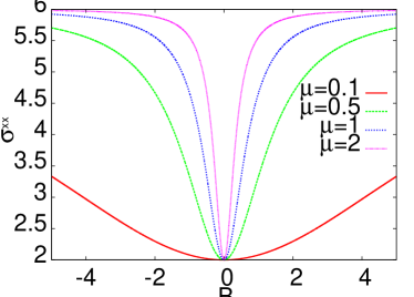
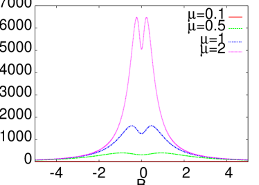
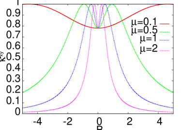
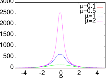
Figure 1: Magnetic field dependence of the conductivity $\sigma^{xx}$ (upper left panel), $\kappa^{xx}$ (upper right panel), thermal conductivity normalized to its maximal value showing more clearly the effect the mobility plays in defining this parameter (lower left panel) and Wiedemann-Franz ratio $W^{xx}$ (lower right panel) at the charge neutrality point $n=0$ for a few values of the mobility $\mu$.

6 Experimental verification

Having in mind the kinetic coefficients matrix (86), we calculated magnetic field dependent transport coefficients, as was explained in the previous section. Experimentally, the results do depend on the sample quality and the studied material. Our model allows to take the sample quality into account only approximately by means of the parameter $\beta$ or the mobility $\mu$. The model in question takes two currents into account and as mentioned earlier they are connected with electrons and holes.

In general they constitute different particle numbers denoted by $Q_{(F)}$ and $Q_{(B)}$. We shall use the parameter $g$ to characterize their relative contribution. We define $Q=Q_{(F)}+Q_{(B)}$ and introduce $g$ by requiring that $Q_{(F)}-Q_{(B)}=gQ$ and identifying $Q$ as the effective carrier concentration $n$. With this choice, motivated by the previous work on graphene seo2017 vanishing of $Q$ is accompanied by vanishing of both $Q_{(F)}$ and $Q_{(B)}$. As already noted it is rather difficult to change $n$ in $(3+1)$-dimensional materials with Dirac spectrum. At the same time the actual concentration of carriers is also not equal to zero. That is why we shall concentrate on the magnetic field dependence of the transport characteristics for the assumed values of $n$. To this end we assume $B_{add}=B$ in what follows. In the equilibrium state and exactly at the Dirac point, one has that $Q=0$. The third free parameter of the model is the coupling $\alpha$ between the two $U(1)$-gauge fields. We shall study the effect of both $g$ and $\alpha$ on the magnetic field dependence for various transport coefficients.

For the perfectly compensated system with $n=0$, all off-diagonal transport coefficients vanish. This can be seen from their definitions, when the effective charge densities go to zero. On the other hand, the following conclusions can be drawn from figure 1. The magneto-resistance (MR) defined as the ratio $MR=(\rho^{xx}(B)-\rho^{xx}(0))/\rho^{xx}(0)$ is always positive if there is no mixing ($g=0$) and no interactions ($\alpha=0$) between currents. The minimal value of the conductivity appears at $B=0$ and does not depend on $\mu$, the effective mobility of carriers. However, the thermal conductivity strongly increases with the growth of the mobility. Moreover, it has a local minimum for $B=0$ and two maxima at finite values of the magnetic field. The lower left panel of the figure shows the decrease of the width of the $\kappa^{xx}$ with increasing of the mobility. The lower right panel of figure 1 shows the Wiedemann - Franz ratio of this compensated system $vs.$ magnetic field. It happens that with the growth of $\mu$, the ratio strongly increases. At the same time, the width of the curve $W^{xx}(B)$ decreases.

Figures 2-5 show the diagonal and off-diagonal components of the thermal conductivity, resistivity, thermoelectric power and Wiedemann-Franz ratio, respectively, as a function of magnetic field calculated for a small but finite value of the carrier concentration $n=0.1$ and for a few values of mobility parameter (as indicated in the figures).

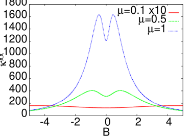
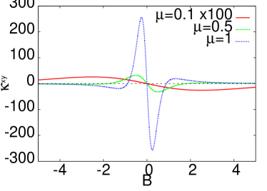
Figure 2: Magnetic field dependence of the thermal conductivity $\kappa^{xx}$ (left panel) and $\kappa^{xy}$ obtained for $g=0$, $\alpha=0$ and charge density $n=0.1$. Different curves correspond to mobility parameter $\mu=0.1,~{}0.5$ and 1. For better visibility we multiplied the curve corresponding to lowest mobilities by the numerical factors 10 or 100.

The maximal values of the thermal conductivity tensor, shown in the figure 2, strongly depend on the mobility $\mu$ also outside the Dirac point. In the figure they are plotted for $n=0.1$, while the other parameters are fixed to be $g=0$ and $\alpha=0$. The component $\kappa^{xx}(B)$ is a symmetric function of the magnetic field, while $\kappa^{xy}$ is antisymmetric with respect to $B$. It turns out that they feature the similar symmetry properties with respect to $n$, $i.e.$ $\kappa^{xx}(-B,~{}-n)=\kappa^{xx}(B,~{}n)$, while $\kappa^{xy}(-B,~{}n)=-\kappa^{xy}(B,~{}n)$ and $\kappa^{xy}(B,~{}-n)=-\kappa^{xy}(B,~{}n)$. The diagonal component has a two peak structure with minimum at $B=0$. The dependence of $\kappa^{xy}$ on the magnetic field is rather complicated. It changes sign for $B=0$ and also for finite $B$. The latter point depends on the mobility and moves towards lower values with the increasing of $\mu$.

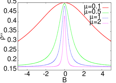
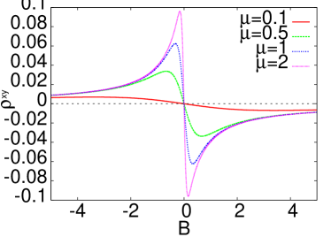
Figure 3: Magnetic field dependence of the diagonal $\rho^{xx}$ (left panel) and off-diagonal $\rho^{xy}$ (right panel) components of the resistivity tensor for a few values of mobility $\mu$. The other parameters are set to $g=0$, $\alpha=0$ and $n=0.1$. Note that the magneto-resistance is negative.

The components of the resistivity tensor are plotted as a function of magnetic field in the figure 3. They possess expected symmetry properties with respect to the magnetic field. The diagonal resistivity is even function of both $B$ and $n$, while $\rho^{xy}$ is odd function of $n$ and also of $B$. With the increase of $\mu$, the width of the curves $\kappa^{xx}(B)$, at half-maximum, narrows. Similarly, the local maxima in $\rho^{xy}$ move towards $B=0$, with the growth of $\mu$. Such a behavior is observed for all the studied transport parameters and seems to be the general feature of the holographic approach to strongly interacting particles. In the studied systems really strong interactions are expected at and the very close distances to the particle-hole symmetry point. The hydrodynamic like behavior is related to the phase space restrictions on the possible single particle scattering events in systems with linear spectrum.

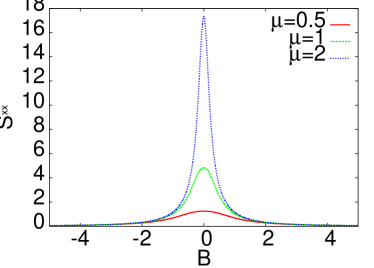
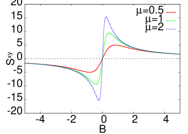
Figure 4: Magnetic field dependence of the diagonal $S^{xx}$ (left panel) and off-diagonal $S^{xy}$ (right panel) components of the t tensor for a few values of mobility $\mu$. The other parameters are set to $g=0$, $\alpha=0$ and $n=0.1$

The Seebeck and Nernst parameters are given by the respective components of the thermoelectric tensor. Phenomenologically they are defined as constants of proportionality between the voltage appearing in the system in response to the applied temperature gradient, with the auxiliary condition that the current vanishes. It is known from condensed matter physics that their measurements give additional information about the spectrum of carriers. In particular, the Seebeck coefficient can be shown to depend on the slope of the density of states at the Fermi energy, while the conductivity depends on the value of the density of states. $S^{xx}$ can also be interpreted as an entropy carried in the system. Figure 4 shows the magnetic field dependence of the Seebeck (left panel) and Nernst components of the thermoelectric tensor. It turns out that $S^{xx}$ is the symmetric function of the magnetic field but antisymmetric function of the charge density $n$. This is in accord with the standard notion that the Seebeck coefficient for electrons is negative and for holes is positive, and its sign is used to define majority carriers. On the other hand, the Nernst coefficient is the even function of $n$ and the odd function of magnetic field $B$.

It is customary to define the Wiedemann-Franz ratio $W^{xx}=\kappa^{xx}/(\sigma^{xx}T)$ and compare its value to the so-called Lorentz constant $L_{0}$, obtained for the nearly free electron model. The departures of $W^{xx}$ from $L_{0}$ ($W^{xx}>L_{0}$) are considered as signs of strongly interacting particles. Here we propose slight extension of the Wiedemann-Franz ratio to both diagonal and non-diagonal components with $W^{xy}=\kappa^{xy}/(\sigma^{xy}T)$. The resulting quantities are plotted in the figure 5, as the function of magnetic field. The three curves correspond to the three values of the mobility and their behavior is in accord with the other transport parameters. Namely, the magnitude increases with the growth of the mobility $\mu$ and the curves narrow down. The diagonal ratio $W^{xx}(B)$ is positive, while $W^{xy}(B)$ changes its sign according to the signs of $\kappa^{xy}(B)$ and $\sigma^{xy}(B)$. The measurements of these ratios for materials with Dirac spectrum would provide the additional test of the holographic approach.

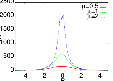
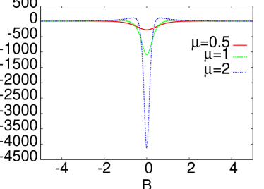
Figure 5: Magnetic field dependence of the Wiedemann-Franz ratio $W^{xx}=\kappa^{xx}/(\sigma^{xx}T)$ (left panel) and $W^{xy}=\kappa^{xy}/(\sigma^{xy}T)$ (right panel) for three values of $\mu=0.5,1,2$ and other parameters set to $n=0.1$, $g=0$ and $\alpha=0$.

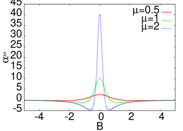
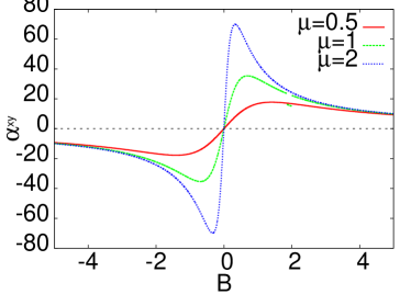
Figure 6: Magnetic field dependence of the thermal kinetic coefficient $\alpha^{xx}$ (left panel) and $\alpha^{xy}$ (right panel) for three values of $\mu=0.5,1,2$ and other parameters set to $n=0.1$, $g=0$ and $\alpha=0$.

Figure 6 illustrates the dependence of the bar values of the thermal conductivities $\alpha^{xx}(B)$ and $\alpha^{xy}(B)$ on the magnetic field, for a few values of the mobility parameter $\mu$. Similarly to the previously discussed transport characteristics, the increase of $\mu$ leads to the growth of the absolute values of different features in these kinetic coefficients.

As mentioned previously, the most often studied 3d system with Dirac spectrum is Cd₃As₂ liang2015 ; liang2017 ; cheng2016 . There have been some experimental measurements of magnetic field dependence of the transport parameters of this material. It is interesting to note that the holographically calculated elements of the conductivity and thermopower tensor show resemblance with the experimental data measured for Cd₃As₂ system liang2015 ; liang2017 . Furthermore, the dependence of the conductivity tensor on the magnetic field features quantitative similarity to the measurement. This is true for the studied material but also for other systems xiong2015 , as it has been reported recently.

We have allowed for the mixing of two currents flowing in the system (parameter $g$) and for their interaction (parameter $\alpha$). The effect of $g$ on some of the studied transport characteristics is shown in the figure 7. The figure envisages the effect of $g$ on the magnetic field dependence of both components of the Wiedemann-Franz ratio. The influence of $g$ is not very big but can be an important factor in the detailed description of experiments. The interaction between the fields $\alpha$ also plays a similar role. It changes the maximal values of various transport parameters as is illustrated in the figure 8, where the longitudinal and Hall resistivities are depicted as the function of the magnetic field. This figure is obtained for $g=0$ but quantitatively similar behavior is observed for $g\neq 0$.

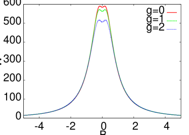
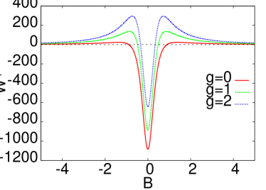
Figure 7: Magnetic field dependence of the Wiedemann-Franz ratio $W^{xx}$ (left panel) and $W^{xy}$ (right panel) for three values of $g=0,1,2$ and other parameters set to $n=0.1$, $g=0$ and $\alpha=0$.

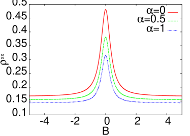
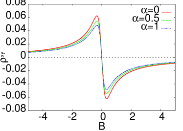
Figure 8: Magnetic field dependence of the resistivity $\rho^{xx}$ (left panel) and $\rho^{xy}$ (right panel) for three values of $\alpha=0,0.5,1$ and other parameters set to $n=0.1$, $g=0$ and $\mu=1$.

The presented calculations are valid for systems which can be considered as a strongly coupled ones. According to the earlier discussion, this condition is expected to be valid relatively close to the Dirac point. In liang2017 both Hall and Nernst effects were analyzed in terms of anomalous contributions arising solely from the Berry phase. Our approach can not quantitatively describe the Berry phase induced contribution to the transport. On the contrary, it gives strong coupling contributions relevant for systems with high mobility.

It is expected that in the studied materials the inter-valley scattering might contribute to the transport. However, unlike the graphene, even strong spin - orbit coupling does not gap the spectrum in DSM. The oscillations of the transport coefficients in high magnetic fields are also envisaged in real systems. However, this effect we do not take into account in the holographic approach. The same is true for the interference effects conjectured due to the Berry phases from electron and hole sheets, at Fermi energy. These are the reasons why our results compare only qualitatively with real data liang2017 .

7 Summary and conclusions

In summary, we have calculated the transport properties of the three dimensional analog of the graphene, usually called Dirac semi-metal (DSM), by using gauge/gravity duality. Motivated by the previous approach to the graphene transport we have generalized the approach by allowing for the mixing of two currents as expressed via the term in the action (1) proportional to $\alpha$. We have also introduced magnetic field ${\bf B=(0,~{}0,~{}B_{z})}$ directed perpendicularly to the electric fields ${\bf E_{F}}$ and ${\bf E_{B}}$ and the temperature gradient $\nabla T$, all applied in the (x,y) plane. The obtained results generalize the known Drude-Boltzmann-like formula to the strong coupling limit. This shows up as an additional term $(\mu B)^{2}~{}(\tilde{Q}_{(F)}\mu r^{2}_{h})^{2}$ appearing in the denominator of the Drude like formula for conductance $\sigma(B)$, where $\mu^{2}=1/(12~{}\beta^{2}~{}r_{h}^{2})$ plays on the holographic side the role of impurity limited mobility of charges in the DSM under consideration.

References

• (1)
• (2)
• (3)
• (4) J.M.Maldacena, The large-N limit of superconformal field theories and supergravity, Adv. Theor. Math. Phys. 2 (1998) 231.
• (5) E.Witten, Anti-de-Sitter space and holography, Adv. Theor. Math. Phys. 2 (1998) 253.
• (6) S.S.Gubser, I.R.Klebanov and A.M.Polyakov, Gauge theory correlators from noncritical string theory, Phys. Lett. B 428 (1998) 105.
• (7) Jan Zaanen, Ya-Wen Sun, Yan Liu and Koenraad Schalm, Holographic Duality in Condensed Matter Physics, Cambridge University Press (2015).
• (8) S.A.Hartnoll, C.P.Herzog and G.T.Horowitz, Building a holographic superconductor, Phys. Rev. Lett. 101 (2008) 031601.
• (9) E. Gubankova, M. Cubrovic, and J. Zaanen, Exciton-driven quantum phase transitions in holography, Phys. Rev. D 92, 086004 (2015)
• (10) P. Kovtun, D. Son and A. Starinets, Viscosity in strongly interacting quantum field theories from black hole physics, Phys. Rev. Lett. 94 (2005) 111601.
• (11) M.Blake and D.Tong, Universal resistivity from holographic massive gravity, Phys. Rev. D 88 (2013) 106004.
• (12) R.A.Davidson, Momentum relaxation in holographic massive gravity, Phys. Rev. D 88 (2013) 086003.
• (13) M.Blake, D.Tong, and D.Vegh, Holographic lattices give the graviton an effective mass, Phys. Rev. Lett. 112 (2014) 071602.
• (14) A.Donos and J.P.Gauntlett, Holographic Q-lattice, JHEP 04 (2014) 040.
• (15) A.Donos and J.P.Gauntlett, Novel metals and insulators from holography, JHEP 06 (2014) 007.
• (16) T.Andrade and B.Withers, A simple holographic model of momentum relaxation, JHEP 05 (2014) 101.
• (17) A.Donos and J.P.Gauntlett, Thermoelectric DC conductivities from black hole horizons, JHEP 11 (2014) 081.
• (18) A.Amoretti, A.Braggio, N.Maggiore, N.Magnoli, and D.Musso, Thermo-electric transport in gauge/gravity models with momentum dissipation, JHEP 09 (2014) 160.
• (19) A.Amoretti, A.Braggio, N.Maggiore, N.Magnoli, and D.Musso, Analytic dc thermoelectric conductivities in holography with massive gravitons, Phys. Rev. D 91 (2015) 025002
• (20) A.Donos and J.P.Gauntlett, Navier-Stokes equations on black hole horizons and DC thermoelectric conductivity, Phys. Rev. D 92 (2015) 121901.
• (21) E.Banks, A.Donos, and J.P.Gauntlett, Thermoelectric DC conductivities and Stokes flows on black hole horizons, JHEP 10 (2015) 103.
• (22) A.Donos, J.P.Gauntlett, T.Griffin, and L.Melgar, DC conductivity of magnetised holographic matter, JHEP 01 (2016) 113.
• (23) A.Donos, J.P.Gauntlett, T.Griffin, and L.Melgar, DC conductivity and higher derivative gravity hep-th 1701.01389 (2017).
• (24) L.Cheng, X.H.Ge, and Z.Y.Sun, Thermoelectric DC conductivities with momentum dissipation from higher derivative gravity, JHEP 04 (2015) 135.
• (25) M.Blake, A. Donos, and N. Lohitsiri, Magnetothermoelectric response from holography, JHEP 08 (2015) 124.
• (26) M. Blake and A. Donos, Quantum critical transport and the Hall angle, Phys. Rev. Lett. 114 (2015) 021601.
• (27) A. Amoretti and D. Musso, Magneto-transport from momentum dissipating holography, JHEP 09 (2015) 094.
• (28) A. Lucas and S. Sachdev, Memory matrix theory of magnetotransport in strange metals, Phys. Rev. B 91 (2015) 195122.
• (29) K. Y. Kim, K.K.Kim, Y.Seo, and S.J.Sin, Thermoelectric conductivities at finite magnetic field and the Nerst effect, JHEP 07 (2015) 027.
• (30) M. S. Foster and I. L. Aleiner, Slow imbalance relaxation and thermoelectric transport in graphene Phys. Rev. B 79, 085415 (2009).
• (31) Y. Seo, G. Song, P. Kim, S. Sachdev, and S.-J. Sin, Holography of the Dirac Fluid in Graphene with Two Currents, Phys. Rev. Lett. 118 (2017) 036601.
• (32) J. Crossno, J. K. Shi, K. Wang, X. Liu, A. Harzheim, A. Lucas, S. Sachdev, P. Kim, T. Taniguchi, K. Watanabe, T. A. Ohki, K. C. Fong, Observation of the Dirac fluid and the breakdown of the Wiedemann-Franz law in graphene, Science 351, (2016) 1058.
• (33) S. M. Young, S.Zaheer, J.C.Y.Teo, C.L.Kane, E.J.Mele, and A.M.Rapee, Dirac Semimetal in Three Dimensions, Phys. Rev. Lett. 108 (2012) 140405.
• (34) A. H. Castro Neto, F. Guinea, N. M. R. Peres, K. S. Novoselov, and A. K. Geim, Rev. Mod. Phys. 81, 109 (2009) The electronic properties of graphene.
• (35) C.Fang, M.J.Gilbert, X.Dai, and B.A.Bernevig, Topological semimetals stabilized by point group symmetry, Phys. Rev. Lett. 108 (2012) 266802.
• (36) B.-J. Yang and N. Nagaosa, Classification of stable three-dimensional Dirac semimetals with nontrivial topology, Nature Commun. 5, (2014) 4989. Nature Commun. 5, 4989 (2014).
• (37) N. P. Armitage, E. J. Mele, A. Vishvanath,Weyl and Dirac Semimetals in Three Dimensional Solids, preprint arXiv:1705:01111 (2017).
• (38) L. Levitov and G. Falkovich, Electron viscosity, current vortices and negative nonlocal resistance in graphene, Nature Physics 12, (2016) 672.
• (39) T. Liang, Q. Gibson, M. N. Ali, M. Liu, R. J. Cava, and N. P. Ong, Ultrahigh mobility and giant magnetoresistance in the Dirac semimetal Cd3As2, Nature Mat. 14, (2015) 280.
• (40) T. Liang, J. Lin, Q. Gibson, T. Gao, M. Hirschberger, M. Liu, R. J. Cava, and N. P. Ong, Anomalous Nernst Effect in the Dirac Semimetal Cd3As2, Phys. Rev. Lett. 118 (2017) 136601.
• (41) L.-P. He and S.-Y. Li, Quantum transport properties of the three- dimensional Dirac semimetal Cd3As2 single crystals, Chin. Phys. B 25, ( 2016) 117105.
• (42) S. Murakami, Phase transition between the quantum spin Hall and insulator phases in 3D: emergence of a topological gapless phase, New J. Phys. 9 (2007) 356.
• (43) D. Hsieh, D. Qian, L. Wray, Y. Xia, Y. S. Hor, R. J. Cava and M. Z. Hasan, A topological Dirac insulator in a quantum spin Hall phase, Nature 452, (2008) 970.
• (44) M. Neupane, S. Y. Xu, R. Sankar, N. Alidoust, G. Bian, C. Liu, I. Belopolski, T. R. Chang, H. T. Jeng, H. Lin, A. Bansil, F. Chou, and M. Z. Hasan, Observation of a three-dimensional topological Dirac semimetal phase in high-mobility Cd3As2, Nature Commun. 5, (2014) 3786.
• (45) M. Neupane, I. Belopolski, M. Mofazzel Hosen, D. S. Sanchez, R. Sankar, M. Szlawska, S-Y. Xu, K. Dimitri, N. Dhakal, P. Maldonado, P. M. Oppeneer, D. Kaczorowski, F. Chou, M. Z. Hasan, and T. Durakiewicz, Observation of topological nodal fermion semimetal phase in ZrSiS, Phys. Rev. B 93 (2016) 201104.
• (46) Z. Wang, Y. Sun, X. Q. Chen, C. Franchini, G. Xu, H. Weng, X. Dai, and Z. Fang, Dirac semimetal and topological phase transitions in A3Bi (A = Na, K, Rb), Phys. Rev. B 85 (2012) 195320.
• (47) Z. Wang, H. Weng, Q. Wu, X. Dai, and Z. Fang, Three-dimensional Dirac semimetal and quantum transport in Cd3As2, Phys. Rev. B 88 (2013) 125427.
• (48) M. Brahlek, N. Bansal, N. Koirala, S. Y. Xu, M. Neupane, C. Liu, M. Z. Hasan, and S. Oh, Topological metal to band-insulator transition in (Bi1-xInx)2Se3 thin films, Phys. Rev. Lett. 109 (2013) 186403.
• (49) L. Wu, M. Brahlek, R. V. Aguilar, A. V. Stier, C. M. Morris, Y. Lubashevsky, L. S. Bilbro, N. Bansal, S. Oh, and N. P. Armitage, A sudden collapse in the transport lifetime across the topological phase transition in (Bi1-xInx)2Se3, Nature Physics 9, (2013) 410
• (50) Z. K. Liu, B. Zhou, Y. Zhang, Z. J. Wang, H. M. Weng, D. Prabhakaran, S. K. Mo, Z. X. Shen, Z. Fang, X. Dai, Z. Hussain, and Y. L. Chen, Discovery of a three-dimensional topological Dirac semimetal, Na3Bi, Science 343, (2014) 864.
• (51) S. Y. Xu, C. Liu, S. K. Kushwaha, R. Sankar, J. W. Krizan, I. Belopolski, M. Neupane, G. Bian, N. Alidoust, T. R. Chang, H. T. Jeng, C. Y. Huang, W. F. Tsai, H. Lin, P. P. Shibayev, F. C. Chou, R. J. Cava, and M. Z. Hasan, Observation of Fermi arc surface states in a topological metal, Science 347, (2015) 294.
• (52) Z. K. Liu, J. Jiang, B. Zhou, Z. J. Wang, Y. Zhang, H. M. Weng, D. Prabhakaran, S. K. Mo, H. Peng, P. Dudin, T. Kim, M. Hoesch, Z. Fang, X. Dai, Z. X. Shen, D. L. Feng, Z. Hussain, and Y. L. Chen, A stable threedimensional topological Dirac semimetal Cd3As2, Nature Mat. 13, (2014) 677.
• (53) H.-Z. Lu and S.-Q. Shen, Quantum transport in topological semimetals under magnetic fields, Front. Phys. 12 (2017) 127201.
• (54) R. Lundgren, P. Laurell and G. A. Fiete, Thermoelectric properties of Weyl and Dirac semimetals, Phys. Rev. B 90 (2014) 165115.
• (55) V. Aji, Adler Bell Jackiw anomaly in Weyl semi-metals: application to pyrochlore iridates, Phys. Rev. B 85 (2012) 241101.
• (56) D. Son and B. Spivak, Chiral anomaly and classical negative magnetoresistance of Weyl metals, Phys. Rev. B 88 (2013) 104412.
• (57) A. Donos and J. P. Gauntlett, Holographic Q lattices, JHEP 4 (2014) 040.
• (58) S.S.Yazadjiev, Generating dyonic solutions in 5D Einstein-dilaton gravity with antisymmetric forms and dyonic black rings, Phys. Rev. D 73 (2006) 124032.
• (59) G.W.Gibbons and K.Maeda, Black holes and membranes in higher-dimensional theories with dilaton fields, Nucl. Phys. B 298 (1988) 741.
• (60) S.Sachdev, What can gauge-gravity duality teach us about condensed matter physics?, Annual Rev. of Cond. Matter Physics 3, (9) 2012.
• (61) J. Gooth et al., Experimental signatures of the mixed axial-gravitational anomaly in the Weyl semimetal NbP, Nature 547, (2017) 324.
• (62) M.Ammon, J.Erdmenger, P.Kerner, and M.Strydom, Black hole instability induced by a magnetic field, Phys. Lett. B 706 (2011) 94.
• (63) S.A.Hartnoll, P.K.Kovtun, M.Müller, and S.Sachdev, Theory of the Nerst effect near quantum phase transition in condensed matter and in dyonic black hole, Phys. Rev. B 76 (2007) 144502.
• (64) P. Cheng, C. Zhang, Y. Liu, X. Yuan, F. Song, Q. Sun, P. Zhou, D. W. Zhang and F. Xiu, Thickness-dependent quantum oscillations in Cd3As2 thin films, New J. Phys. 18 (2016) 083003.
• (65) J. Xiong, S. Kushwaha, J. Krizan, T. Liang, R. J. Cava, and N. P. Ong, Anomalous conductivity tensor in the Dirac semimetal Na3Bi, EPL 114 (2016) 27002.