Abstract

In a recent paper [1], we had advanced a minimal resolution of some of the persistent anomalies in semileptonic $B$-decays. These include the neutral-current observables $R_{K}$ and $R_{K^{*}}$, as well as the charged-current observables $R(D)$ and $R(D^{*})$. Recently, it has been observed that the semileptonic decays of the $B_{c}$ meson also hint at a similar type of anomaly. In this longer version, we discuss in detail why, if the anomalies are indeed there, it is a challenging task to explain the data consistently in terms of a simple and compelling new physics scenario. We find that the minimal scheme to achieve a reasonable fit involves the inclusion of just two (or, at worst, three with a possible symmetry relationship between their Wilson coefficients) new current-current operators, constructed in terms of the flavour eigenstates, augmented by a change of basis for the charged lepton fields. With only three unknown parameters, this class of models not only explain all the anomalies (including that in $B_{c}\to J/\psi\,\ell\nu$) to a satisfactory level but also predict some interesting signatures, like $B\to K\mu\tau$, $B_{s}\to\tau\tau$, $B\to K$ plus missing energy, or direct production of $\tau^{+}\tau^{-}$, that can be observed at LHCb or Belle-II.

Keywords: Flavour anomalies, New physics signals, Lepton mixing

1 Introduction

The last few years have seen some intriguing hints of discrepancies in a few charged- as well as neutral-current decays of $B$-mesons, when compared to the expectations within the Standard Model (SM). While the fully hadronic decay modes are subject to large (and, in cases, not-so-well understood) strong interaction corrections, the situation is much more under control for semileptonic decays, where the dominant uncertainties come from the form factors and quark mass values. Even these uncertainties are removed to a large extent if one considers ratios of similar observables. Thus, the modes $b\to c\ell\overline{\nu}$ and $b\to s\ell^{+}\ell^{-}$ are of great interest. While, individually, none of these immediately calls for the inclusion of New Physics (NP) effects (given the current significance levels of the discrepancies), viewed together, they strongly suggest that some NP is lurking around the corner (see, e.g., Ref. [2]). Most interestingly, the pattern also argues convincingly for some NP that violates lepton-flavour universality (LFU), a cornerstone of the SM. The violation is to a level that cannot be simply explained by the inclusion of right-handed neutrino fields and the consequent neutrino masses; indeed, the strength is only a little over an order of magnitude below that generated from the weak scale dynamics.

As we have just mentioned, relative partial widths (or, equivalently, the ratios of branching ratios (BR)) are particularly clean probes of physics beyond the SM, on account of the cancellation of the leading uncertainties inherent in individual BR predictions. Of particular interest to us are the ratios $R(D)$ and $R(D^{*})$ pertaining to charged-current decays, defined as

$$R(D^{(*)})\equiv\frac{{\rm BR}(B\to D^{(*)}\tau\nu)}{{\rm BR}(B\to D^{(*)}\ell\nu)}\,,$$ (1)

with $\ell=e$ or $\mu$, the ratio $R_{J/\psi}$ defined as

$$R_{J/\psi}\equiv\frac{{\rm BR}(B_{c}\to J/\psi\,\tau\nu)}{{\rm BR}(B_{c}\to J/\psi\,\mu\nu)}\,,$$ (2)

and analogous ratios for the neutral-current sector

$$R_{K^{(*)}}\equiv\frac{{\rm BR}(B\to K^{(*)}\mu^{+}\mu^{-})}{{\rm BR}(B\to K^{(*)}e^{+}e^{-})}\,.$$ (3)

For the $K^{*}$ mode, the discrepancy is visible not only in the ratios of binned differential distribution for muon and electron mode, but also in some angular asymmetries in $B\to K^{*}\mu\mu$ which we discuss later.

The SM estimates for these decays are already quite robust. With the major source of uncertainty being the form factors, they cancel out in ratios like $R(D^{(*)})$, $R_{J/\psi}$, or $R_{K^{(*)}}$. The values of $R(D)$ and $R(D^{*})$ as measured by BABAR [3], when taken together, exceed SM expectations by more than $3\sigma$. While the Belle measurements lie in between the SM expectations and the BABAR measurements and are consistent with both [4], their result on $R(D^{*})$ [5], with the $\tau$ decaying semileptonically, agrees with the SM expectations only at the $1.6\sigma$ level. Similarly, the first measurement by LHCb [7] is also $2.1\sigma$ above the SM prediction. Considering the myriad results together, and including the correlations, the tension between data and SM is at the level of $4.1\sigma$ [9].

While the data on $R(D)$ and $R(D^{*})$ lie above the SM predictions, those on $R_{K}$ and $R_{K^{*}}$ are systematically below the expectations. A similar shortfall has been observed in the $q^{2}\in[1:6]$ GeV² bin for the decay $B_{s}\to\phi\mu\mu$, which is again mediated by the process $b\to s\mu\mu$. However, no appreciable discrepancy is found between the data on the purely leptonic decay $B_{s}\to\mu^{+}\mu^{-}$ and the radiative decay $B\to X_{s}\gamma$, and the corresponding SM expectations. The same is true for the mass difference $\Delta M_{s}$ and mixing phase $\phi_{s}$ measurements for the $B_{s}$ system. The pattern of deviations is thus a complicated one and, naively at least, seemingly contradictory. These, therefore, pose an interesting challenge to the model builders: how to incorporate all the anomalies in a model with the least number of free parameters?

While both model-dependent and model-independent search strategies for NP based on $R_{K}$ and/or $R(D^{(*)})$ data are being discussed in the literature for a while now [10, 11], the subject has recently received a further impetus from the announcement of the apparent deficit in $R_{K^{*}}$ [12]. There has been a flurry of activity trying to explain the $R_{K}$ and $R_{K^{*}}$ anomalies within the context of such models, or in a model-independent framework [13]. However, only a handful of them try to explain both $R_{K^{(*)}}$ and $R(D^{(*)})$ anomalies together [14]. Unfortunately, either the models are not minimal in nature, or the fits are not very good. Following our earlier rather concise work [1] of a bottom-up model-independent explanation of both the anomalies, we will explain, in this paper, the framework in detail, and also expand the earlier study significantly.

Rather than advocating a particular model, we shall assume a very phenomenological approach. Virtually all the data can be explained in terms of an effective Lagrangian, operative at low-energies, and different from that obtained within the SM. However, with ‘minimality’ being a criterion, we would like to follow the principle of Occam’s razor and not introduce an arbitrarily large number of new parameters, as would be the case with a truly anarchic effective theory. The issue of operator mixing and possible generation of new operators at the scale $m_{b}$ is also nontrivial, as shown in Ref. [15]. Rather than considering the complete set of dimension-6 current-current operators and obtaining the best fit to all data, our approach could be deemed as an attempt for an inspired guess for the minimal set of operators that still produces a more than satisfactory fit, yet with small values of the Wilson coefficients (WC). If the NP scale is not beyond a few TeVs, the aforementioned operator mixing would be small and the WCs of any new operator generated as a quantum corrections would be tiny. The best fit for the WCs, thus obtained, would presumably pave the way for inspired model building. We will show how the relationship between the NP WCs may hold the key for a yet unknown flavour dynamics.

As the reader would have noticed, we have considered only the operators built out of vector and axial-vector currents alone. This is solely because our aim has been to correlate the charged-current and the neutral-current anomalies and demonstrate that they may have originated from the same source. While the charged-current anomalies in $R(D)$ and $R(D^{*})$ can possibly be addressed with scalar and/or tensor current operators while evading the strong constraints arising from the lifetime of the $B_{c}$ meson [16], such operators are not of much help for $R_{K^{(*)}}$. For example, it has widely been discussed in the literature that if the only new operators are those constructed with (pseudo)scalar currents, the explanation for $R_{K}$ would be incompatible with the data on $B_{s}\to\ell^{+}\ell^{-}$. Similarly, the viability of tensor operators in the case of the neutral current anomalies is discussed in Ref. [11]. Once one deviates from the assumption of minimality, it is indeed possible to have different Lorentz structures of the NP operators. While this may actually occur in some specific NP models, in the absence of a well-motivated ultraviolet-complete theory, such an Ansatz would militate against the spirit of Occam’s razor.

The rest of the paper is arranged as follows. In Sec. 2, we recount and discuss the experimental situation. This is followed, in Sec. 3, by a discussion of the microscopic dynamics that lead to such processes. Sec. 4 discusses a model that could have explained the data but falls short narrowly. This is followed, in Sec. 5, by a discussion of more realistic scenarios. Sec. 6 contains our results, and finally we conclude in Sec. 7.

2 The data : a brief recounting

We begin by briefly reviewing the experimental measurements and theoretical predictions for the observables of interest. We also take this opportunity to review some further processes that would turn out to have important consequences in our attempt to explain the anomalies.

• As already mentioned, discrepancies in the measurements of the observables $R(D)$ and $R(D^{*})$ have been seen, over the last several years, in multiple experiments such as LHCb, BABAR  and Belle. In Table. 1, taken from Ref.[17], we summarize the measurements along with the corresponding SM predictions.

  	${R}(D)$	${R}(D^{*})$
  SM prediction	$0.300\pm 0.008$ [18]	$0.252\pm 0.003$ [19]
  BABAR  (Isospin constrained)	$0.440\pm 0.058\pm 0.042$	$0.332\pm 0.024\pm 0.018$ [3]
  Belle (2015)	$0.375\pm 0.064\pm 0.026$	$0.293\pm 0.038\pm 0.015$ [4]
  Belle (2016)	—	$0.302\pm 0.030\pm 0.011$ [5]
  Belle (2016, Full)	—	$0.270\pm 0.035~{}^{+0.028}_{-0.025}$ [6]
  LHCb (2015)	—	$0.336\pm 0.027\pm 0.030$ [7]
  LHCb (2017)	—	$0.285\pm 0.019\pm 0.029$ [8]
  Average	$0.407\pm 0.039\pm 0.024$	$0.304\pm 0.013\pm 0.007$ [9]

  Table 1: The SM predictions for and the data on $R(D)$ and $R(D^{*})$. While BABAR considers both charged and neutral $B$ decay channels, LHCb and Belle results, as quoted here, are based only on the analysis of neutral $B$ modes. For Belle, ‘Full’ implies the inclusion of both semileptonically and hadronically tagged samples, the last-mentioned excluded otherwise. The average is from HFLAV [9].

  $R(D)$ and $R(D^{*})$ exceed their respective SM predictions by $2.3\sigma$ and $3.4\sigma$. Taking the correlation into effect, the discrepancy is at the level of $4.1\sigma$ [9]. Thus,

  $$R(D)=(1.36\pm 0.15\,)\times R(D)_{\text{SM}},\qquad\qquad R(D^{*})=(1.21\pm 0.06\,)\times R(D^{*})_{\text{SM}}\ .$$ (4)

  At this point, let us mention that recently two groups have published their own calculations of $R(D^{*})_{\rm SM}$, namely, $0.260\pm 0.008$ [20] and $0.257\pm 0.005$ [21]. While these estimates reduce the tension slightly, to $2.3\sigma$ [20] and $2.9\sigma$ [21] respectively, note that the error bars are somewhat bigger. Given that the consequent changes in numerical estimates are minimal, we will continue to use the results of Ref. [19] in the main, but would also indicate the change the results that would be wrought by the use of the new calculations.

• Recently, the LHCb collaboration has observed the hint of another discrepancy [23] for the same quark-level transition $b\to c\tau\overline{\nu}$ but in the $B_{c}$ meson system. With only the spectator quark changing, the SM analysis would be very similar to that for $R(D^{*})$, with the main modification accruing from the change in the phase-space factors. Much the same would be true for a large class of new physics scenarios, wherein the tensorial structure of the effective four-fermion operators remain essentially unchanged. Analyzing $3\,{\rm fb}^{-1}$ data, The LHCb Collaboration found

  $$R_{J/\psi}=\left\{\hskip-5.0pt\begin{array}[]{lcl}\displaystyle 0.71\pm 0.17\pm 0.18&\hskip-5.0pt&({\rm exp.}),\\[8.61108pt] \displaystyle 0.283\pm 0.048&\hskip-5.0pt&({\rm SM})\,.\end{array}\right.$$ (5)

  The SM prediction [24, 25, 26] includes the uncertainties coming from the $B_{c}\to J/\psi$ form factors and, thus, is quite robust. Given the relatively low production cross section for the $B_{c}$ meson, the uncertainty in the measurement is still large and the discrepancy is just below the $2\sigma$ level. With the accumulation of more data, not only would the statistical uncertainties reduce, even the systematics are expected to come down on account of a better understanding of the same. While the present level of the discrepancy is not a very significant one, it is interesting to note that it points in the same direction as the other charged-current decays.

• For the neutral current transitions (pertaining to $b\to s\ell^{+}\ell^{-}$), we have [27, 12]:

  $$\begin{array}[]{rclcl}R_{K}&=&\displaystyle 0.745^{+0.090}_{-0.074}\pm 0.036&&\displaystyle q^{2}\in[1:6]\,{\rm GeV}^{2}\,,\\[8.61108pt] R_{K^{*}}^{\text{\,low}}&=&\displaystyle{0.66}^{+0.11}_{-0.07}\pm 0.03&&\displaystyle q^{2}\in[0.045:1.1]\,{\rm GeV}^{2}\,,\\[8.61108pt] R_{K^{*}}^{\text{\,central}}&=&\displaystyle 0.69^{+0.11}_{-0.07}\pm 0.05&&q^{2}\in[1.1:6]\,{\rm GeV}^{2}\,.\end{array}$$ (6)

  The SM predictions for both $R_{K}$ and $R_{K^{*}}^{\text{\,central}}$ are virtually indistinguishable from unity [28], whereas for $R_{K^{*}}^{\text{\,low}}$ it is $\sim$ 0.9 (due to the finite lepton mass effect). These calculations are very precise with negligible uncertainties associated with them. Thus the measurements of $R_{K}$, $R_{K^{*}}^{\text{\,low}}$ and $R_{K^{*}}^{\text{\,central}}$, respectively, correspond to $2.6\sigma$, $2.1\sigma$ and $2.4\sigma$ deviations from the SM predictions.

• Another hint of deviation (at a level of more than $3\sigma$), for a particular neutral-current decay mode is evinced by $B_{s}\to\phi\mu\mu$  [29, 30, 31].

  $$\frac{d~{}}{dq^{2}}{\rm BR}(B_{s}\to\phi\mu\mu){\Big{|}}_{q^{2}\in[1:6]\,{\rm GeV}^{2}}=\left\{\begin{array}[]{lcl}\displaystyle\left(2.58^{+0.33}_{-0.31}\pm 0.08\pm 0.19\right)\times 10^{-8}~{}{\rm GeV}^{-2}&&({\rm exp.})\\[8.61108pt] \displaystyle\left(4.81\pm 0.56\right)\times 10^{-8}~{}{\rm GeV}^{-2}&&({\rm SM})\,.\end{array}\right.$$ (7)

  where $q^{2}=m^{2}_{\mu\mu}$. Intriguingly, the $q^{2}$ region where this measurement has relatively low error (and data is quoted) is virtually the same as that for $R_{K}$ and $R_{K^{*}}^{\text{\,central}}$. This measurement, thus, suggests strongly that the discrepancies in $R_{K}$ and $R_{K^{*}}$ have been caused by a depletion of the $b\to s\mu^{+}\mu^{-}$ channel, rather than an enhancement in $b\to se^{+}e^{-}$. This is further vindicated by the long-standing $P^{\prime}_{5}$ anomaly [32] in the angular distribution of $B\to K^{*}\mu\mu$, which again occurs in the central $q^{2}$ region, with the mismatch between data and SM prediction being more than $3\sigma$.

• Such a conclusion, though, has to be tempered with the data for the corresponding two-body decay, viz. $B_{s}\to\mu^{+}\mu^{-}$. The theory predictions are quite robust now, taking into account possible corrections from large $\Delta\Gamma_{s}$, as well as next-to-leading order (NLO) electroweak and next-to-next-to-leading order (NNLO) QCD corrections. The small uncertainty essentially arises from the corresponding Cabibbo-Kobayashi-Maskawa (CKM) matrix elements and the decay constant of $B_{s}$. The recent measurement of LHCb at a significance of $7.8\sigma$ [33, 34] shows an excellent agreement between the data and the SM prediction:

  $$\text{BR}(B_{s}\to\mu^{+}\mu^{-})=\left\{\begin{array}[]{lcl}\displaystyle\left(3.0\pm 0.6^{+0.3}_{-0.2}\right)\times{10}^{-9}&&({\rm exp.}),\\[8.61108pt] \displaystyle\left(3.65\pm 0.23\right)\times 10^{-9}&&({\rm SM})\,,\end{array}\right.$$ (8)

  and hence puts very strong constraints on NP models, in particular on those incorporating (pseudo-)scalar currents (this has also been noted in Ref. [35]). Of course, as the data shows, a small depletion $\sim 20\%$ in the rates is still allowed, and, indeed, to be welcomed. NP operators involving only vector currents do not affect this channel, but scalar, pseudoscalar, and axial vector operators do.

For future reference, we list here three further rare decay modes.

• Within the SM, the decay modes $b\to s\nu_{i}\overline{\nu}_{i}$ are naturally suppressed, owing to the fact that these are generated by either an off-shell $Z$-mediated diagram coupling to a flavour-changing quark-vertex, or through box-diagrams. Interestingly, the current upper bounds (summed over all three neutrinos) as obtained by the Belle collaboration [36], viz.

  $${\rm BR}(B\to K\nu\overline{\nu})<1.6\times 10^{-5}\,,\qquad\quad{\rm BR}(B\to K^{*}\nu\overline{\nu})<2.7\times 10^{-5}$$ (9)

  (both at 90% C.L) are not much weaker than what is expected within the SM, namely [37]

  $$\begin{array}[]{rcl}\displaystyle{\rm BR}(B^{+}\to K^{+}\nu\overline{\nu})_{\rm SM}&=&\displaystyle(3.98\pm 0.43\pm 0.19)\times 10^{-6}\ ,\\[8.61108pt] \displaystyle{\rm BR}(B^{+}\to K^{*0}\nu\overline{\nu})_{\rm SM}&=&\displaystyle(9.19\pm 0.86\pm 0.50)\times 10^{-6}\ .\end{array}$$ (10)

  In other words, we have

  $$\frac{{\rm BR}^{\rm exp}_{K}}{{\rm BR}^{\rm SM}_{K}}<3.9\,,\qquad\quad\frac{{\rm BR}^{\rm exp}_{K^{*}}}{{\rm BR}^{\rm SM}_{K}}<2.7\,.$$

• The purely leptonic mode $B_{s}\to\tau\tau$ is yet to be observed but LHCb put a 95% confidence level bound on the BR [38]:

  $${\rm BR}(B_{s}\to\tau^{+}\tau^{-})<6.8\times 10^{-3}\,.$$ (11)

  The SM prediction, of course, is way too small, $(7.73\pm 0.49)\times 10^{-7}$ [34].

• The limits on the rare lepton flavour violating modes $B\to K\mu\tau$ [39] are

  $${\rm BR}(B^{+}\to K^{+}\mu^{+}\tau^{-})<4.5\times 10^{-5}\,,\ \ {\rm BR}(B^{+}\to K^{+}\mu^{-}\tau^{+})<2.8\times 10^{-5}\,.$$ (12)

Finally, the direct production of $\tau^{+}\tau^{-}$ pairs at the LHC was well-measured for both the 8 TeV and the 13 TeV runs [40]. This serves to constrain the WCs of any effective theory giving rise to a $\tau^{+}\tau^{-}$ final state Refs. [41, 42].

3 Operators relevant to the observables

Having delineated, in the preceding section, the observables of interest, we now proceed to the identification of the operators, within the SM and beyond, responsible for effecting the transitions. As the scale of NP surely is above the electroweak scale, we will talk in terms of effective current-current operators that, presumably, are obtained by integrating out the heavy degrees of freedom, and not confine ourselves within any particular model. To be precise, the genesis of these operators will be left to the model builders.

Given the fact that, even within the SM, the neutral-current decays under consideration occur only as loop effects, several current-current operators would, in general, be expected to contribute to a given four-fermion amplitude. However, as we shall soon see, certain structures have a special role. To this end, we introduce a shorthand notation:

$$(x,y)\equiv\overline{x}_{L}\gamma^{\mu}y_{L}\ \ \ \ \forall\ \ x,y\,.$$ (13)

3.1 The $b\to c\tau\overline{\nu}_{\tau}$ transition

This proceeds through a tree-level $W$-exchange in the SM. If the NP adds coherently to the SM, one can write the effective Hamiltonian as

$${\cal H}^{\text{eff}}=\frac{4G_{F}}{\sqrt{2}}V_{cb}\left(1+C^{\mathrm{NP}}\,\right)\,\left[(c,b)(\tau,\nu_{\tau})\right]\,,$$ (14)

where the NP contribution, parametrized by $C^{\mathrm{NP}}\,$, vanishes in the SM limit. Using Eq. (1), we can write

$$\frac{{R(D^{(*)})}_{\text{SM+NP}}}{{R(D^{(*)})}_{\text{SM}}}=\left|1+C^{\mathrm{NP}}\,\right|^{2}.$$ (15)

Thus, to explain the data, one needs either small positive values, or large negative values, of $C^{\mathrm{NP}}\,$.

On the other hand, if the NP involves an operator with a different Lorentz structure, or with different field content (like $b\to c\tau\overline{\nu}_{\mu}$), the addition would be incoherent in nature, and the relative phase of $C^{\mathrm{NP}}\,$ is immaterial. More crucially, though, this would alter the functional form of the differential width. An identical situation arises for $R_{J/\psi}$.

3.2 The $b\to s\mu^{+}\mu^{-}$ transition

Responsible for the FCNC decays $B\to K^{(*)}\mu^{+}\mu^{-}$ and $B_{s}\to\phi\mu^{+}\mu^{-}$, within the SM, this transition proceeds, primarily, through two sets of diagrams, viz. the “penguin-like” one (driven essentially by the top quark) and the “box” (once again, dominated by the top). It is, thus, convenient to parametrize the ensuing effective Hamiltonian as

$${\cal H}^{\text{eff}}=\frac{-4G_{F}}{\sqrt{2}}\,V_{tb}\,V_{ts}^{*}\,\sum_{i}C_{i}(\mu)\mathcal{O}_{i}(\mu)\,,$$ (16)

where the relevant operators are

$$\mathcal{O}_{7}=\frac{e}{16\pi^{2}}m_{b}\left(\overline{s}\sigma_{\mu\nu}P_{R}b\right)F^{\mu\nu}\,,\ \ \mathcal{O}_{9}=\frac{e^{2}}{16\pi^{2}}\left(\overline{s}\gamma_{\mu}P_{L}b\right)\left(\overline{\mu}\gamma^{\mu}\mu\right)\,,\ \ \mathcal{O}_{10}=\frac{e^{2}}{16\pi^{2}}\left(\overline{s}\gamma_{\mu}P_{L}b\right)\left(\overline{\mu}\gamma^{\mu}\gamma_{5}\mu\right)\,.$$ (17)

The WCs, matched with the full theory at $m_{W}$ and then run down to $m_{b}$ with the renormalisation group equations at the next-to-next-to-leading logarithmic (NNLL) accuracy [43], are given in the SM as $C_{7}=-0.304\,,\ \ C_{9}=4.211\,,\ \ C_{10}=-4.103\,.$ If the NP operators are made only with (axial)vector currents, one can denote the modified WCs as

$$C_{9}\to C_{9}+C_{9}^{\mathrm{NP}}\,=4.211+C_{9}^{\mathrm{NP}}\,\,,\ \ \ C_{10}\to C_{10}+C_{10}^{\mathrm{NP}}\,=-4.103+C_{10}^{\mathrm{NP}}\,\,.$$ (18)

The consequent normalized differential branching fraction for the $B\to K\mu^{+}\mu^{-}$ decay in terms of the dimuon invariant mass squared, $q^{2}$, is given by

$$\frac{1}{\Gamma_{0}}\frac{d\Gamma(B\to K\mu^{+}\mu^{-})}{dq^{2}}\! = \!2\lambda^{1/2}(m_{B}^{2},m_{K}^{2},q^{2})\sqrt{1-\frac{4m_{\mu}^{2}}{q^{2}}}\Bigg{\{}\frac{1}{6}\lambda(m_{B}^{2},m_{K}^{2},q^{2})\left(1+\frac{2m_{\mu}^{2}}{q^{2}}\right)\left(|F_{A}|^{2}+|F_{V}|^{2}\right)$$ (19)

$$+ \!q^{2}|F_{P}|^{2}+4m_{\mu}^{2}m_{B}^{2}|F_{A}|^{2}+2m_{\mu}\left(m_{B}^{2}-m_{K}^{2}+q^{2}\right)\text{Re}(F_{P}F_{A}^{*})\Bigg{\}},$$

where

$$\Gamma_{0}=\frac{G_{F}^{2}\alpha^{2}}{2^{9}\pi^{5}m_{B}^{3}}|V_{tb}V_{ts}^{*}|^{2},~{}{\rm and}~{}~{}\lambda(a,b,c)\equiv a^{2}+b^{2}+c^{2}-2(ab+bc+ac)$$

is the famed phase-space factor. The functions $F_{i}$ depend on the WCs and $q^{2}$ dependent form factors $f_{0,+,T}$ of the $B\to K$ transition [44], namely

$$\begin{array}[]{rcl}F_{P}&=&\displaystyle-m_{\mu}\left(C_{10}+C_{10}^{\mathrm{NP}}\,\right)\,\left[f_{+}(q^{2})-\frac{m_{B}^{2}-m_{K}^{2}}{q^{2}}\left(f_{0}(q^{2})-f_{+}(q^{2})\right)\right]\ ,\\[12.91663pt] F_{A}&=&\displaystyle\left(C_{10}+C_{10}^{\mathrm{NP}}\,\right)\,f_{+}(q^{2})\ ,\\[10.76385pt] F_{V}&=&\displaystyle\left(C_{9}+C_{9}^{\mathrm{NP}}\,\right)f_{+}(q^{2})+2C_{7}\,m_{b}\,\frac{f_{T}(q^{2})}{m_{B}+m_{K}}\ .\end{array}$$ (20)

The differential distribution for the $B\to V\ell\ell$ mode, where $V$ stands for a $K^{*}$ or $\phi$ meson, can be expressed in terms of certain angular coefficients $I_{i}$ [45] as

$$\frac{d\Gamma(B\to V\mu^{+}\mu^{-})}{dq^{2}}=\frac{1}{4}\left[3I_{1}^{c}(q^{2})+6I_{1}^{s}(q^{2})-I_{2}^{c}(q^{2})-2I_{2}^{s}(q^{2})\right]$$ (21)

The coefficients $I_{i}$ are functions of the transversity amplitudes $\mathcal{A}^{L,R}_{\lambda,t}$ where $\lambda$ denotes the three states of polarisations of the meson $V$, and $L$ and $R$ denote the left and right chirality of the lepton current, respectively. We refer to Appendix A for the detailed expressions of $I_{i}$ and $\mathcal{A}^{L,R}_{\lambda,t}$.

3.3 The $b\to s\nu\overline{\nu}$ transition

Quite akin to the preceding case, this transition (which governs the $B\to K^{(*)}\nu\overline{\nu}$ decay) proceeds through both $Z$-penguin and box diagrams. Unless NP introduces right-handed neutrino fields, the low energy effective Hamiltonian may be parametrised by [37]

$${\cal H}^{\text{eff}}=-\frac{4G_{F}}{\sqrt{2}}\,V_{tb}\,V_{ts}^{*}\,\frac{\alpha_{\rm em}}{4\pi}\,C_{L}^{\text{SM}}\,\left(1+C_{\nu}^{\mathrm{NP}}\,\right)\,\times 2\,(s,b)(\nu,\nu),$$ (22)

where $\alpha_{\rm em}$ is the fine structure constant and $C_{\nu}^{\mathrm{NP}}\,$denotes the NP contribution. Including NLO QCD corrections and the two loop electroweak contribution, the SM WC is given by $C_{L}^{\text{SM}}=-X_{t}/s_{w}^{2}$ where $X_{t}=1.469\pm 0.017$ [46, 37].

3.4 The two-body decay rates

The branching fraction for $B_{s}^{0}\to\ell^{+}\ell^{-}$, where $\ell$ is any charged lepton, can be written, at the leading order, as

$${\rm BR}(B_{s}^{0}\to\ell^{+}\ell^{-})=\frac{G_{F}^{2}\alpha^{2}m_{B_{s}}\tau_{B_{s}}f_{B_{s}}^{2}m_{\ell}^{2}}{16\pi^{3}}|V_{tb}V_{ts}^{*}|^{2}\sqrt{1-\frac{4m_{\ell}^{2}}{m_{B_{s}}^{2}}}~{}\left|C_{10}+C_{10}^{\mathrm{NP}}\,\right|^{2}\,,$$ (23)

while that for $B_{c}^{-}\to\tau^{-}\nu_{\tau}$ is given by

$${\rm BR}(B_{c}^{-}\to\tau^{-}\nu_{\tau})=\frac{G_{F}^{2}m_{B_{c}}\tau_{B_{c}^{-}}f_{B_{c}}^{2}m_{\tau}^{2}}{8\pi}|V_{cb}|^{2}\left(1-\frac{m_{\tau}^{2}}{m^{2}_{B_{c}}}\right)^{2}\left|1+C^{\mathrm{NP}}\,\right|^{2}\,,$$ (24)

where $m_{B}$, $\tau_{B}$ and $f_{B}$ are the mass, lifetime and decay constant of the relevant $B$ meson respectively. We assume an identical operator structure leading to coherent addition of the amplitudes.

4 Semi-realistic scenarios

In the spirit of effective theories, a “model” in our discussions would correspond to only a combination of (at most) two four-fermi operators at the scale $m_{b}$. We, expressly, do not venture to obtain the ultraviolet (UV) completion thereof, leaving this for future studies. We also assume that the NP scale is low enough, maybe at a few TeV, so that higher-loop corrections do not generate any new operator of significant strength, leading to, e.g., the purely leptonic decay $\tau\to 3\mu$. Our aim, thus, is to identify the smallest set of couplings that are phenomenologically viable. To begin with, we present a model that we call semi-realistic, because while it can explain all other anomalies, it is inconsistent with the constraint coming from the decay $B_{s}\to\tau^{+}\tau^{-}$.

This instructive exercise would allow us to pinpoint the structure that NP must lead to so as both explain the anomalies as well as satisfy all other constraints. We will follow this, in the next section, by constructing appropriate realistic scenarios.

Clearly, any such operator should, at the very least, respect the (gauged) symmetries of the SM. On the other hand, since the data explicitly calls for lepton-flavour violation, the latter cannot be a symmetry of the NP operator(s). Such a violation can accrue from a plethora of NP scenarios, such as models of (gauged) flavour, leptoquarks (or, within the supersymmetric paradigm, a breaking of $R$-parity) etc. Let us here investigate a structure that could, in principle, be motivated from such theories.

The data in question calls for the effect of NP to be concentrated in effective operators straddling the second and third generations. On the other hand, any such effective Hamiltonian accruing from a NP scale higher than the electroweak scale (as it must be, on account of the colliders, past and present, not having seen such resonances), can only be written in terms of the weak-interaction eigenstates [47]. The breaking of the electroweak symmetry, aided by non-diagonal Yukawa couplings, would, in general, induce extra operators even if we started with a single one. While some of these effects would be trivial (and aligned with the usual CKM rotations), this is not necessarily true for all. We will exploit this in striving to explain all the anomalies starting from a minimal set. In particular, our operators will involve second and third generation quark fields, to account for the $b\to c$ and $b\to s$ transitions, but only the third generation lepton fields, with the charged lepton state appropriately rotated to give rise to the mass eigenstates of $\mu$ and $\tau$ leptons.

4.1 The could-have-been model

Let us consider the following set of operators:

$${\rm Model~{}I:}\qquad\mathcal{O}_{\rm I}=\sqrt{3}\,A_{1}\,(\overline{Q}_{2L}\gamma^{\mu}L_{3L})_{3}\,(\overline{L}_{3L}\gamma_{\mu}Q_{3L})_{3}-2\,A_{2}\,(\overline{Q}_{2L}\gamma^{\mu}L_{3L})_{1}\,(\overline{L}_{3L}\gamma_{\mu}Q_{3L})_{1}\,.$$ (25)

where $A_{1,2}$ are the WCs, and $Q_{i}$ and $L_{i}$ denote the usual $i$-th generation (and weak-eigenstate) $SU(2)_{L}$ quark and lepton doublet fields respectively. The subscript ‘3’ and ‘1’ denote that the currents are $SU(2)_{L}$ triplets and singlets, respectively, whereas the factor of $\sqrt{3}$ has been introduced explicitly to account for the Clebsch-Gordan coefficients. It should be noted that only the second and third generation quark doublets and the third generation lepton doublet alone are involved in Eq. (25), as mentioned earlier. Considering the simplest of field rotations for the left-handed leptons from the unprimed (flavour) to the primed (mass) basis, namely

$$\tau=\cos\theta\,\tau^{\prime}+\sin\theta\,\mu^{\prime}\ ,\qquad\quad\nu_{\tau}=\cos\theta\,\nu_{\tau}^{\prime}+\sin\theta\,\nu_{\mu}^{\prime}\,.$$ (26)

terms with the potential to explain the $b\to s\mu\mu$ anomalies are generated.

The best fit values for these can be obtained by effecting a $\chi^{2}$-test defined through

$$\chi^{2}=\sum_{i=1}^{8}\frac{\left(\mathcal{O}_{i}^{\text{exp}}-\mathcal{O}_{i}^{\text{th}}\right)^{2}}{\left(\Delta\mathcal{O}_{i}^{\text{exp}}\right)^{2}+\left(\Delta\mathcal{O}_{i}^{\text{th}}\right)^{2}}$$ (27)

where $\mathcal{O}_{i}^{\text{exp}}$ and $\Delta\mathcal{O}_{i}^{\text{exp}}$ are the experimental mean and $1\sigma$ uncertainty in the measurements and $\Delta\mathcal{O}_{i}^{\text{th}}$ is the theoretical uncertainty in the observables. The observables $\mathcal{O}_{i}^{\text{th}}$ are calculated within Model I and thus depend on the model parameters. We include a total of eight measurements for the evaluation of $\chi^{2}$, namely, $R(D),~{}R(D^{*})$ (from Eq. (4)), $R_{J/\psi}$ (from Eq. (5)) $R_{K},~{}R_{K^{*}}^{\text{\,low}},~{}R_{K^{*}}^{\text{\,central}}$ (from Eq. (6)), the integrated $\text{BR}(B_{s}\to\phi\mu\mu)$ for the range $q^{2}\in[1:6]\,{\rm GeV}^{2}$ (from Eq. (7)) and $\text{BR}(B_{s}\to\mu\mu)$ (from Eq. (8)). The theoretical uncertainties $\Delta\mathcal{O}_{i}^{\text{th}}$, however small, are taken into account for all observables. For our numerical analysis, we use

$$V_{cb}=0.0416\ ,\qquad V_{tb}V_{ts}^{*}=-0.0409\ ,\qquad s_{w}^{2}=0.22\,,$$

and find, for the SM, $\chi^{2}_{\rm SM}/{\rm d.\,o.\,f.}\simeq 6.1$. For Model I, on the other hand, the minimum value is $\chi^{2}_{\rm min}/{\rm d.\,o.\,f.}\simeq 1.5$ denoting a remarkable improvement from the SM value. The fit results are

$$A_{1}=0.028~{}{\rm TeV}^{-2}\,,\ \ A_{2}=-2.90~{}{\rm TeV}^{-2}\,,\ \ |\sin\theta|=0.018\,,$$ (28)

leading to

$${\rm BR}(B^{+}\to K^{+}\nu\overline{\nu})=6.1\times 10^{-6}\,,\ \ {\rm BR}(B\to K^{*}\nu\overline{\nu})=1.4\times 10^{-5}\,.$$ (29)

Note that the small value of $A_{1}$ means that at the matching scale of the effective theory, $A_{1}$ could very well be zero, making this a two-parameter model ($A_{2}$ and $\sin\theta$). The fit would have improved significantly if we exclude $R_{K^{*}}^{\text{\,low}}$ from our analysis. The BRs for $B\to K\mu\tau$ and $B\to K^{*}\mu\tau$ [48] increase to $2.1\times{10}^{-5}$ and $3.6\times{10}^{-5}$ respectively, just below the current observed limit (see Eq. (12)).

The NP contribution to the WCs $C_{9}^{\mathrm{NP}}\,$, $C_{10}^{\mathrm{NP}}\,$and $C^{\mathrm{NP}}\,$come out to be

$$C_{9}^{\mathrm{NP}}\,=-C_{10}^{\mathrm{NP}}\,=-0.61\ ,\qquad C^{\mathrm{NP}}\,=-2.11\ .$$ (30)

Not only is this completely consistent with the global fit results for $b\to s$ transitions, but also provides an explanation for the well known $P_{5}^{\prime}$ [32] anomaly as it calls for an (axial)vector contribution to the muon mode with similar coupling strength [30].

We come, finally, to the decay mode that rules out this model, namely $B_{s}\to\tau^{+}\tau^{-}$. The theoretical expression for this mode is given in Eq. (23). It can be ascertained that the typical value of the BR as predicted within Model I is an order of magnitude higher than the LHCb limit quoted before [38]. Indeed, the only way the $B_{s}\to\tau^{+}\tau^{-}$ constraint can be satisfied is to tweak the values of the WCs to an extent that the best fit value for $R_{K^{*}}$ is nearly $2\sigma$ away from the global average, thereby negating the very essence of the effort. Depending on the structure of the UV-complete theory, one may even have a similar large contribution, in stark contrast to the data, to the mass difference $\Delta M_{s}$ for the $B_{s}$ system. This issue is discussed at a later stage.

At the same time, let us note that the LHCb collaboration has, very recently, announced measurement of $R(D^{*})$ through the 3-prong decay of the $\tau$ [49], with this particular data being consistent with the SM expectations at about $1\sigma$. More importantly, while the global average of $R(D^{*})$ reduces, its deviation from the SM value actually increases marginally to $\sim 3.4\sigma$ [49] on account of the improved precision. This movement of the global average allows for the adoption of smaller values for $A_{i}$, thereby reducing the tension with $B_{s}\to\tau^{+}\tau^{-}$. Indeed, if $R(D^{*})$ were to be entirely dominated by this new measurement, or the BR for $B_{s}\to\tau^{+}\tau^{-}$ were found to be larger than the LHCb limit, the tension would be reduced to acceptable levels and this model would have worked fine.

Before we proceed further, let us mention that one can construct similar models, like

$${\rm Model~{}II:}\qquad\mathcal{O}_{\rm II} = -\sqrt{3}\,A_{1}\,(\overline{Q}_{2L}\gamma^{\mu}Q_{3L})_{3}\,(\overline{L}_{3L}\gamma_{\mu}L_{3L})_{3}+\sqrt{3}\,A_{2}\,(\overline{Q}_{2L}\gamma^{\mu}L_{3L})_{3}\,(\overline{L}_{3L}\gamma_{\mu}Q_{3L})_{3}\ ,$$ (31)

$${\rm Model~{}III:}\qquad\mathcal{O}_{\rm III} = -\sqrt{3}\,A_{1}\,(\overline{Q}_{2L}\gamma^{\mu}Q_{3L})_{3}\,(\overline{L}_{3L}\gamma_{\mu}L_{3L})_{3}+2\,A_{3}\,(\overline{Q}_{2L}\gamma^{\mu}Q_{3L})_{1}\,(\overline{L}_{3L}\gamma_{\mu}L_{3L})_{1}\,,$$ (32)

while all these models satisfy every constraint and yield similar $\chi^{2}_{\rm min}$, they all fail to keep BR($B_{s}\to\tau^{+}\tau^{-}$) within the allowed limit.

We, nonetheless, endeavour below to identify a scenario that is not dependent on wishful thinking, as aforementioned.

5 Realistic models

The strong constraints from $\Delta M_{s}$ and $B_{s}\to\tau^{+}\tau^{-}$, as seen in the preceding section, emanated from the fact that, in each of the cases, we generated a substantial $C_{10}^{\rm NP}$, namely a NP contribution to the operator $\mathcal{O}_{10}$ for the tauonic mode (in Eq. (17))

$$\frac{e^{2}}{16\pi^{2}}\left(\overline{s}\gamma_{\mu}P_{L}b\right)\left(\overline{\tau}\gamma^{\mu}\gamma_{5}\tau\right)\ .$$

Indeed, we consistently had $C_{10}^{\rm NP}=-C_{9}^{\rm NP}$. While the operator $\mathcal{O}_{9}$ has only a vanishing contribution to the decay, the situation is very different for $\mathcal{O}_{10}$. Although the latter contribution suffers a chirality suppression, it is still substantial for $B_{s}\to\tau^{+}\tau^{-}$. Thus, consistency with this mode would require $C_{10}^{\rm NP}$ to be small.

On the other hand, a substantial change in $R_{K^{(*)}}$ would require at least one of $C_{10}^{\rm NP}$ and $C_{9}^{\rm NP}$ to be substantial. In other words, we must break the relation $C_{10}^{\rm NP}=-C_{9}^{\rm NP}$, which was a consequence of working, thus far, with left-handed currents alone. Learning from the lessons of the preceding section, we now consider simple variants of the models already introduced.

5.1 Model IV

Consider the following set of operators

$$\begin{array}[]{rcl}{\cal O}_{\rm IV}&=&\displaystyle\sqrt{3}\,A_{1}\,\left[-(\overline{Q}_{2L}\gamma^{\mu}Q_{3L})_{3}\,(\overline{L}_{3L}\gamma^{\mu}L_{3L})_{3}+\frac{1}{2}\,(\overline{Q}_{2L}\gamma^{\mu}L_{3L})_{3}\,(\overline{L}_{3L}\gamma^{\mu}Q_{3L})_{3}\right]\\[8.61108pt] &+&\displaystyle\sqrt{2}\,A_{5}\,(\overline{Q}_{2L}\gamma^{\mu}Q_{3L})_{1}\,(\overline{\tau}_{R}\gamma^{\mu}\tau_{R})\ ,\end{array}$$ (33)

where the new WC $A_{5}$ (note that the factor of $\sqrt{2}$ is a Clebsch-Gordan factor) parametrizes the strength of the right-handed tauonic current. In terms of the component field, this reduces to

$$\begin{array}[]{rcl}{\cal O}_{\rm IV}&=&\displaystyle\frac{3\,A_{1}}{4}\,(c,b)\,(\tau,\nu_{\tau})+\frac{3\,A_{1}}{4}(s,b)(\tau,\tau)+A_{5}\,(s,b)\,\{\tau,\tau\}\\[8.61108pt] &+&\displaystyle\frac{3\,A_{1}}{4}\,(s,t)\,(\nu_{\tau},\tau)+A_{5}(c,t)\{\tau,\tau\}+\frac{3\,A_{1}}{4}(c,t)\,(\nu_{\tau},\nu_{\tau})\end{array}$$ (34)

where we have introduced the shorthand notation

$$\{x,y\}\equiv\overline{x}_{R}\gamma^{\mu}y_{R}\ \ \ \ \forall\ \ x,y\,,$$ (35)

and the terms in the second line of eqn.(34) are irrelevant for the processes in hand. Clearly, $A_{5}\simeq 3A_{1}/4$ would suppress any NP contribution to $B_{s}\to\tau^{+}\tau^{-}$. Simultaneously, this will automatically generate a tiny contribution to $B\to K^{(*)}\mu^{+}\mu^{-}$, comparable with the SM contribution, without needing to tune the leptonic mixing angle to an unnaturally small value. Note that we have already imposed the symmetry that had led to the suppression of the $B\to K^{(*)}\overline{\nu}\nu$ modes.

While the introdution of the right-handed current opens the possibility of introducing an independent mixing matrix for the right-handed leptons, we eschew this in the interest of having the fewest parameters in the NP sector. This would also be the case for the other model discussed below.

5.2 Model V

The analogous change in Model II and in Model III would, interestingly, result in the same set of operators as

$$\begin{array}[]{rcl}{\cal O}_{\rm V}&=&\displaystyle-\sqrt{3}\,A_{1}\,(\overline{Q}_{2L}\gamma^{\mu}Q_{3L})_{3}\,(\overline{L}_{3L}\gamma^{\mu}L_{3L})_{3}+A_{1}\,(\overline{Q}_{2L}\gamma^{\mu}Q_{3L})_{1}\,(\overline{L}_{3L}\gamma^{\mu}L_{3L})_{1}\\[8.61108pt] &+&\displaystyle\sqrt{2}\,A_{5}\,(\overline{Q}_{2L}\gamma^{\mu}Q_{3L})_{1}\,(\overline{\tau}_{R}\gamma^{\mu}\tau_{R})\end{array}$$ (36)

leading to

$$\begin{array}[]{rcl}{\cal O}_{\rm V}&=&\displaystyle A_{1}\,(c,b)\,(\tau,\nu_{\tau})+A_{1}\,(s,b)\,(\tau,\tau)+A_{5}\,(s,b)\,\{\tau,\tau\}\\[8.61108pt] &+&\displaystyle A_{1}\,(s,t)\,(\nu_{\tau},\tau)+A_{1}\,(c,t)(\nu_{\tau},\nu_{\tau})+A_{5}\,(c,t)\,\{\tau,\tau\}\end{array}$$ (37)

with the first line containing all terms of relevance. Once again, the (symmetry) relation between the coefficients of the first two operators helps evade constraints from $B\to K^{(*)}\overline{\nu}\nu$. Moreover, the very structure of Eq. (37) suggests that $A_{5}\simeq A_{1}$ would be preferred by $B_{s}\to\tau^{+}\tau^{-}$.

6 Results

The fitting of NP operators progress in exact analogy with that in Sec. 4.1, with the relaxation of the condition $C_{10}^{\rm NP}=-C_{9}^{\rm NP}$. Whereas the $\chi^{2}$ (defined in Eq. (27)) is still minimized for $|\sin\theta|\simeq 0.018$, such a solution would not simultaneously satisfy both of BR$(B^{+}\to K^{+}\mu^{-}\tau^{+})$ as well as BR$(B_{s}\to\tau^{+}\tau^{-})$ and yet lead to a satisfactory solution for the other variables. Consequently, the best fit is obtained for a slightly different value, namely

$$|\sin\theta|\simeq 0.016$$ (38)

applicable to each case. We now have $\chi^{2}_{\text{min}}/{\rm d.\,o.\,f.}=1.7$, a rise of 1.3 from the unconstrained minimum. The new best fit values of the WCs are

$$C_{9}^{\text{NP}}=-0.35\ ,\qquad C_{10}^{\text{NP}}=0.55\ ,\qquad C^{\text{NP}}=-2.11\ .$$

This shows a marked improvement from the SM value of $\chi^{2}/{\rm d.\,o.\,f.}=6.1$. It should be noted that even this low value of $\chi^{2}_{\rm min}/{\rm d.\,o.\,f.}=1.7$ is dominated by a single measurement, namely, $R_{K^{*}}^{\text{\,low}}$. Indeed, for the best fit points of the NP parameter space, we have $R_{K^{*}}^{\text{\,low}}=0.83$ which is a little more than $1\sigma$ way from the LHCb measurement. This is quite akin to the various other studies in the literature [13] who too have concluded that an agreement to this experimental value to better than $1\sigma$ is not possible if the NP contribution can be expressed just as a modification of the SM Wilson coefficients. Rather, it necessitates the introduction of a new dynamical scale altogether. Having determined $\sin\theta$ as above, we choose, for illustrative purposes, to relax the conditions imposed by ${\rm BR}(B^{+}\to K^{+}\mu^{-}\tau^{+})$ as well as ${\rm BR}(B_{s}\to\tau^{+}\tau^{-})$. This would allow us to choose the best fit values for the parameters in each of the two cases. These are displayed in Table 2.

Best fit points	Model IV	Model V
$|$sin$\theta|$	$0.016$	$0.016$
$A_{1}$ in TeV-2	$-3.88$	$-2.91$
$A_{5}$ in TeV-2	$-2.61$	$0.66$

Table 2: Central values of the fitted parameters for the two models.

In Fig. 1, we depict the $95\%$ and $99\%$ C.L. bands, in the plane of the WCs, around the new best fit point. Also shown are the regions in the parameter space allowed by the upper limits on ${\rm BR}(B_{s}\to\tau^{+}\tau^{-})$ (the orange shaded region) and ${\rm BR}(B^{+}\to K^{+}\mu^{-}\tau^{+})$ (the yellow shaded region). The former, as expected, is truly restrictive. The overlap region, thus, denotes the viable parameter space at a given confidence level.

The observables at the overlap region, corresponding to a least value of $\chi^{2}/{\rm d.\,o.\,f.}\simeq 2.6$, are given by

$$\begin{array}[]{rcl}R_{K}&=&0.80\ ,\\[4.30554pt] R_{K^{*}}^{\text{low}}&=&0.88\ ,\\[4.30554pt] R_{K^{*}}^{\text{central}}&=&0.83\ ,\\[4.30554pt] R(D)&=&0.36\ ,\\[4.30554pt] R(D^{*})&=&0.30\ ,\\[4.30554pt] R_{J/\psi}&=&\displaystyle 0.34\ ,\\[4.30554pt] \displaystyle\frac{d}{dq^{2}}\text{BR}(B_{s}\to\phi\mu\mu)&=&3.8\times 10^{-8}\,{\rm GeV}^{-2}~{}~{}\mbox{for}\quad q^{2}\in[1:6]\,{\rm GeV}^{2}\ .\end{array}$$ (39)

From Fig. 1, one might be led to think that the models IV and V are consistent only at 95% C.L. or worse, but this is deceptive. It should be noted that the contours shown in Fig. 1 are not drawn around the absolute minimum of $\chi^{2}$, which, in any case, is incompatible with other data, namely, $B^{+}\to K^{+}\mu^{-}\tau^{+}$ and $B_{s}\to\tau^{+}\tau^{-}$. Yet, the $\chi^{2}$ values corresponding to the overlap region, namely $\raisebox{-1.72218pt}{\hbox to0.0pt{$\sim$\hss}}\raisebox{1.72218pt}{$<$}15\,(18)$ for the 95% (99%) C.L. bands, are much better than that obtained within the SM, which is $\sim 49$. In other words, the improvement is remarkable.

It has been shown in Ref. [50] that the inclusion of left-handed NP current in the $b\to c\tau\overline{\nu}_{\tau}$ transition to explain the $R(D^{(*)})$ anomalies, does not jeopardize the lifetime of the $B_{c}$ meson significantly, although it opens up an annihilation mode $B_{c}\to\tau\nu$ for its decay. Our results for NP coefficients correspond to a modification of $\sim 3\%$ of the lifetime and is well within the allowed limit.

We also make a couple of strong predictions which should be tested in LHCb in near future. First, for both the models under consideration, the similar ratio in $B_{s}\to\phi\ell^{+}\ell^{-}$ mode, namely, $R_{\phi}\equiv{\rm BR}(B_{s}\to\phi\mu^{+}\mu^{-})/{\rm BR}(B_{s}\to\phi e^{+}e^{-})$ should be less than unity and is predicted to be $\simeq 0.83$ for the range $q^{2}\in[1:6]\,{\rm GeV}^{2}$. Second, as the allowed region almost saturates the bounds arising from the modes ${\rm BR}(B_{s}\to\tau^{+}\tau^{-})$ and ${\rm BR}(B^{+}\to K^{+}\mu^{-}\tau^{+})$, they should also be observable in near future, and so should be $B\to K^{*}\tau\mu$. Apart from this, several anomalous top decay channels may be probed at the LHC or the next generation $e^{+}e^{-}$ collider. Each of these predictions provides independent modes to both test and falsify the scenarios proposed.

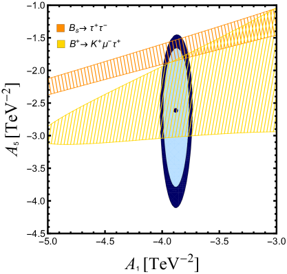
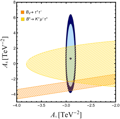
Figure 1: The viable parameter space for two different models i.e., model IV and model V are shown in left and right panel, respectively. The point represents the minimum of the $\chi^{2}$, whereas the light and dark blue ellipses denote $95\%$ and $99\%$ C.L. regions, respectively. The orange and yellow shaded regions are allowed by the BR$(B_{s}\to\tau^{+}\tau^{-})$ and BR$(B^{+}\to K^{+}\mu^{-}\tau^{+})$ bounds. The overlaps denote the finally allowed portion of the parameter space.

6.1 Caveat: Quantum corrections and new operators

While the issue of too large a ${\rm BR}(B_{s}\to\tau^{+}\tau^{-})$ faced by the semi-realistic scenarios discussed in Sec. 4 was taken care of in the models proposed in Sec. 5, a further issue remains.

The operators that we discussed can also, in principle, generate new contributions to $B_{s}$–$\overline{B_{s}}$ mixing. Consider, e.g. the $\tau$-loop diagram contributing to the effective $\Delta B=\Delta S=2$ operator. The amplitude is formally a quadratically divergent one. Thus, to calculate it one needs to introduce a cutoff $\Lambda$ which could be estimated by parametrizing $A_{i}=a_{i}/\Lambda^{2}$ with $a_{i}\sim{\cal O}(1)$. In other words, the fit dictates $\Lambda$ to be a few TeV at most. Using $\Lambda$ as a cutoff would, naively, generate a WC that only scales with $\Lambda^{-2}$. In other words, we seemingly have[51]

$$\frac{\zeta}{\Lambda^{2}}\,(\overline{b}\,\gamma_{\mu}\,P_{L}\,s)\,(\overline{b}\,\gamma^{\mu}\,P_{L}\,s)\qquad\quad\zeta\sim{\cal O}\left(\frac{a_{i}^{2}}{\pi^{2}}\right)\,.$$ (40)

Accepting this, the experimental measurement of the mass difference $\Delta M_{s}$ imposes a rather strong constraint, namely, $A_{1}\,\raisebox{-1.72218pt}{\hbox to0.0pt{$\sim$\hss}}\raisebox{1.72218pt}{$<$}\,0.1\,{\rm TeV}^{-2}$ [51], and this limit falls linearly with increasing $\Lambda$. This apparent conflict with our fit results can be evaded if there are more contributions to the $B_{s}$–$\overline{B_{s}}$ mixing. A trivial example is provided by postulating a “tree-level” operator with a form identical to that above and a coefficient with a sign opposite to $\zeta$ above. A more interesting alternative could be to appeal to some yet-to-be-discovered symmetry of the full theory that cancels out, at least approximately, all the quantum corrections to the existing set of dimension-6 operators that may lead to a sizable $\Delta M_{s}$. Either solution could, of course, be termed a slightly fine-tuned one.

Before we delve deeper into this problem, it behoves us to consider the very calculation of $\zeta$ indicated above. One criticism is that the result is dependent on the regularisation prescription and a different one could have resulted in a markedly different $\zeta$. A more subtle issue pertains to the very nature of such calculations in an effective theory. Indeed, an effective Lagrangian is presumably the result of either having integrated out the heavy fields in a more fundamental theory or having incorporated (some of) the quantum corrections to yield an effective action. If the local Lagrangian under consideration is to be thought of as the lowest order approximation in an expansion, further quantum corrections due to the UV physics alone can only result in corrections to the WCs and not generate any new terms in the Lagrangian. Such new terms should arise only when quantum corrections to low-energy physics are taken into account.

In the present context, if say the operator ${\cal O}_{V}$ were the result of a $Z^{\prime}$ exchange, then the operator of Eq. (40) should have been generated at the same level as ${\cal O}_{V}$. Suppressing $B_{s}$–$\overline{B}_{s}$ mixing would, then, require that the $bsZ^{\prime}$ coupling be far smaller than the $\tau\tau Z^{\prime}$ one. Calculating the $\tau$-loop would, then, be unnecessary and largely meaningless. On the other hand, imagine that the operator ${\cal O}_{V}$ was generated as a combined effect of a slew of coloured fields (with the displayed form being the result of a final Fierz rearrangement). In such a case, the operator of Eq. (40) would be generated only when mixed loops involving both these coloured (and heavy) fields as well as the SM bosons. Intricately woven with this are dependence on the light masses and the analogue of the GIM cancellations. With the attendant additional suppression, by a factor of $\alpha_{\rm wk}\,m_{\rm light}^{2}/\Lambda^{2}$ where $m_{\rm light}$ is the typical mass of the SM fields, the consequent value of $\zeta$ is small enough for our effective Lagrangian to be in consonance with $B_{s}$–$\overline{B}_{s}$ mixing. In other words, this constraint should be considered as only an indicative one, perhaps pointing to the nature of the UV completion.

Thus, we are brought back to the assertion implicit in the entire discussion of this paper, namely that there has to exist some symmetry in the UV-complete theory that ensures that the discussed operators (in a given scenario) constitute the entire set appearing at the lowest order in the said EFT. The Wilson coefficients of any other four-fermion operator generated as a result of quantum corrections must, necessarily, be suppressed by at least $\alpha_{\rm wk}\,m_{\rm light}^{2}/\Lambda^{2}$. Such a suppression, of course, would render the scenario safe from the perspective of $\Delta M_{s}$.

Very similar to the discussion above is the case for $\tau\to 3\mu$, putatively generated by a quark loop.

7 Conclusion

In this paper, we identify the minimal extension of the SM in terms of effective four-fermion operators that can explain two sets of anomalies: $R_{K}$ and $R_{K^{*}}$ on the one hand, as well as $R(D)$, $R(D^{*})$ and $R_{J/\psi}$ on the other. Explaining both sets at a single stroke has been challenging for two reasons: $(i)$ there is a deficiency in the former case but an excess in the latter, and $(ii)$ because they involve different leptons, viz. muons for the first pair and $\tau$s for the second.

The final state leptons, though, can be related by postulating a small rotation of the original charged lepton field involved in the dimension-6 operator(s). With the very inclusion of a flavour-nonuniversal operator, such a rotation is no longer a trivial one (as is the case with the SM). With the neutrino flavour in such decays not being observed, only the incoherent sum over states is a measurable quantity. As for excesses in both the neutral- and charged-current processes, these are related by the usual $SU(2)_{L}$ symmetry.

Based on these principles, we have formulated several scenarios with a minimal set of dimension-6 gauge and Lorentz invariant operator. The “models” have at most three parameters, namely the WCs corresponding to the effective operators (two or less) and the lepton mixing angle.

Taking all the data into account, we find that two such operators are enough to get an acceptable fit. For the best fit points, all the observables, barring $R_{K^{*}}^{\rm low}$ and ${\rm BR}(B_{s}\to\phi\mu\mu)$ in the low-$q^{2}$ bin, are consistent within $1\sigma$. (For the latter, the agreement is better than $2\sigma$.) Even for the standout observable (for which the data is still not of great quality), the disagreement is only slightly worse than $1\sigma$. In addition, we can also explain the observed suppression in the low-$q^{2}$ bins for the decay $B_{s}\to\phi\mu\mu$.

A strong prediction of our analysis is that either $B\to K\mu\tau$ and/or $B_{s}\to\tau^{+}\tau^{-}$ will be close to discovery, and one should look for such channels in LHCb as well as Belle-II. At the same time, we do not attempt to probe the origin of these new operators; while a $Z^{\prime}$ or a vector leptoquark may do the job, this is left for the model builders.

Although we start with a simplistic scenario with two operators in each case, it is conceivable that a hitherto unknown symmetry relates the two unknown WCs. Indeed the choices $A_{2}=A_{1}/2$, applicable for Models I and II, are strikingly simple, and conceivably, may arise from some unidentified flavour dynamics. Such a symmetry, if exact, would lead to a vanishing NP contribution (at the tree level in the effective theory) to the $b\to s\nu\overline{\nu}$ amplitude. However, quantum corrections would be expected to break this symmetry. Although such rates would be small, they should still be visible at Belle-II.

Model I is interesting from a different perspective. The best-fit value of the WC $A_{1}$ is two-orders of magnitude below the other, namely $A_{2}$. Indeed, this is one case where a single operator does almost as well as two together, or in other words, only two parameters for the new physics are required here. This is a remarkably simple solution to all of the disparate set of anomalies that confront us. A slight modified version of this case has been discussed in Ref. [1], where the bounds from $B_{s}\to\tau\tau$ are well under control. Most interestingly, the scale of the new (flavour) physics is suggested to be a few TeVs at best, rendering the situation extremely attractive for the current run of the LHC.

It has to be noted, though, that the recent LHCb bound on $B_{s}\to\tau^{+}\tau^{-}$ rules out the simplest of the scenarios. While this measurement is crucially dependent on the use of neural networks etc. (as the $\tau$s are yet to be fully reconstructed) and the consequent uncertainties, it is worthwhile to investigate if the suppression of the $C_{10}^{\rm NP}$ contribution that it calls for, can be accommodated in such scenarios. We find that this can indeed be done without the introduction of additional parameters, but at the cost of introducing an additional gauge invariant operator, whose WC is envisaged to be related with the other WCs by some yet-to-be-discovered symmetry. While the $\chi^{2}$ worsens marginally, it is still miles better than that in the SM. The models have a few generic predictions, like the possibility of observing $B\to K^{(*)}\mu\tau$ or $B_{s}\to\tau^{+}\tau^{-}$ in near future, and possibly $B\to K^{(*)}$ plus missing energy. They will definitely be checked within the next couple of years at LHCb, and Belle-II will be able to make precision studies on these observables. The other features of the scenarios, including the possibility of direct observation of TeV-scale resonances at the LHC, remain unaltered.

The authors thank Gino Isidori and Sudhendu RaiChoudhury for illuminating discussions. AK thanks the Science and Engineering Research Board (SERB), Government of India, for a research grant. DC acknowledges partial support from the European Union’s Horizon 2020 research and innovation program under Marie Skłodowska–Curie grant No 674896.

Appendix A Appendix

The expressions for the angular coefficients present in the differential distribution of $B\to V\ell^{+}\ell^{-}$ decay, discussed in Sec. 3, are

$$I_{1}^{s} =\frac{(2+\beta^{2})}{4}\Big{[}|{{\cal A}_{\perp}^{L}}|^{2}+|{{\cal A}_{\parallel}^{L}}|^{2}+(L\to R)\Big{]}+\frac{4m^{2}}{q^{2}}\text{Re}({{\cal A}_{\perp}^{L}}{{\cal A}_{\perp}^{R}}^{*}+{{\cal A}_{\parallel}^{L}}{{\cal A}_{\parallel}^{R}}^{*}),$$ (41)

$$I_{1}^{c} =|{{\cal A}_{0}^{L}}|^{2}\!+\!|{{\cal A}_{0}^{R}}|^{2}\!+\!\frac{4m^{2}}{q^{2}}\big{[}\left|{\cal A}_{t}\right|^{2}\!+\!2\text{Re}({{\cal A}_{0}^{L}}{{\cal A}_{0}^{R}}^{*})\big{]},$$ (42)

$$I_{2}^{s} =\frac{\beta^{2}}{4}\Big{[}|{{\cal A}_{\perp}^{L}}|^{2}+|{{\cal A}_{\parallel}^{L}}|^{2}+(L\to R)\Big{]},$$ (43)

$$I_{2}^{c} =-\beta^{2}\Big{[}|{{\cal A}_{0}^{L}}|^{2}+(L\to R)\Big{]}.$$ (44)

Here, the transversity amplitudes $\mathcal{A}^{L,R}_{0,\|,\perp,t}$ are functions of the Wilson coefficients and the form factors $V(q^{2})$, $A_{0,1,2}(q^{2})$ and $T_{1,2,3}(q^{2})$ for $B\to V$ transitions. The expressions are

$$\mathcal{A}_{\perp}^{L,R} =N\sqrt{2}\lambda^{1/2}\left\{\left[\left(C_{9}+C_{9}^{\mathrm{NP}}\,\right)\mp\left(C_{10}+C_{10}^{\mathrm{NP}}\,\right)\right]\frac{V(q^{2})}{m_{B}+m_{V}}+\frac{2m_{b}}{q^{2}}C_{7}T_{1}(q^{2})\right\},$$ (45)

$$\mathcal{A}_{\|}^{L,R} =-N\sqrt{2}\left(m_{B}^{2}-m_{V}^{2}\right)\left\{\left[\left(C_{9}+C_{9}^{\mathrm{NP}}\,\right)\mp\left(C_{10}+C_{10}^{\mathrm{NP}}\,\right)\right]\frac{A_{1}(q^{2})}{m_{B}-m_{V}}+\frac{2m_{b}}{q^{2}}C_{7}T_{2}(q^{2})\right\},$$ (46)

$$\mathcal{A}_{0}^{L,R} =-\frac{N}{2m_{V}\sqrt{q^{2}}}\Bigg{\{}\left[\left(C_{9}+C_{9}^{\mathrm{NP}}\,\right)\mp\left(C_{10}+C_{10}^{\mathrm{NP}}\,\right)\right]$$

$$\hskip 56.9055pt\times\left[\left(m_{B}^{2}-m_{V}^{2}-q^{2}\right)\left(m_{B}+m_{V}\right)A_{1}(q^{2})-\lambda\frac{A_{2}(q^{2})}{m_{B}+m_{V}}\right]$$

$$\hskip 56.9055pt+2m_{b}C_{7}\left[\left(m_{B}^{2}+3m_{V}^{2}-q^{2}\right)T_{2}(q^{2})-\lambda\frac{T_{3}(q^{2})}{m_{B}^{2}-m_{V}^{2}}\right]\Bigg{\}},$$ (47)

$$\mathcal{A}_{t} =\frac{N}{\sqrt{q^{2}}}\lambda^{1/2}\,2\left(C_{10}+C_{10}^{\mathrm{NP}}\,\right)A_{0}(q^{2}),$$ (48)

where          $N=V_{tb}V_{ts}^{*}\Big{[}\displaystyle\frac{G_{F}^{2}\alpha^{2}}{3\times 2^{10}\,\pi^{5}\,m_{B}^{3}\,}q^{2}\,\lambda^{1/2}\,\beta\Big{]}^{1/2}$,          with $\beta=\sqrt{1-4m_{\mu}^{2}/q^{2}}$,

and $\lambda\equiv\lambda(m_{B}^{2},m_{V}^{2},q^{2})=m_{B}^{4}+m_{V}^{4}+q^{4}-2(m_{B}^{2}m_{V}^{2}+m_{V}^{2}q^{2}+m_{B}^{2}q^{2})$.

References

- [1] D. Choudhury, A. Kundu, R. Mandal and R. Sinha, Phys. Rev. Lett. 119, 151801 (2017) [arXiv:1706.08437 [hep-ph]].
-
[2]
W. Altmannshofer and D.M. Straub,
Eur. Phys. J. C 73, 2646 (2013)
[arXiv:1308.1501 [hep-ph]];
S. Descotes-Genon, J. Matias and J. Virto, Phys. Rev. D 88, 074002 (2013) [arXiv:1307.5683 [hep-ph]];
B. Bhattacharya, A. Datta, D. London and S. Shivashankara, Phys. Lett. B 742, 370 (2015) [arXiv:1412.7164 [hep-ph]];
R. Mandal and R. Sinha, Phys. Rev. D 95, 014026 (2017) [arXiv:1506.04535 [hep-ph]];
A. Karan, R. Mandal, A. K. Nayak, R. Sinha and T. E. Browder, Phys. Rev. D 95, 114006 (2017); arXiv:1603.04355 [hep-ph]. - [3] J. P. Lees et al. [BaBar Collaboration], Phys. Rev. D 88, 072012 (2013) [arXiv:1303.0571 [hep-ex]].
- [4] M. Huschle et al. [Belle Collaboration], Phys. Rev. D 92, 072014 (2015) [arXiv:1507.03233 [hep-ex]].
- [5] A. Abdesselam et al. [Belle Collaboration], arXiv:1603.06711 [hep-ex].
- [6] S. Hirose et al. [Belle Collaboration], arXiv:1612.00529 [hep-ex].
- [7] R. Aaij et al. [LHCb Collaboration], Phys. Rev. Lett. 115, 111803 (2015) [Phys. Rev. Lett. 115, 159901 (2015) (E)] [arXiv:1506.08614 [hep-ex]].
-
[8]
G. Wormser, talk given at FPCP 2017, Prague, and available at
https://indico.cern.ch/event/586719/contributions/2531261/attachments/1470695/2275576/2_fpcp_talk_wormser.pdf -
[9]
Y. Amhis et al.,
arXiv:1612.07233 [hep-ex] and the update at
http://www.slac.stanford.edu/xorg/hflav/semi/fpcp17/RDRDs.html -
[10]
C. Bobeth, T. Ewerth, F. Kruger and J. Urban,
Phys. Rev. D 64, 074014 (2001)
[hep-ph/0104284];
W. Altmannshofer, P. Ball, A. Bharucha, A. J. Buras, D. M. Straub and M. Wick, JHEP 0901, 019 (2009) [arXiv:0811.1214 [hep-ph]];
G. Hiller and M. Schmaltz, Phys. Rev. D 90, 054014 (2014) [arXiv:1408.1627 [hep-ph]];
A. Crivellin, C. Greub and A. Kokulu, Phys. Rev. D 86, 054014 (2012) [arXiv:1206.2634 [hep-ph]];
A. Crivellin, G. D’Ambrosio and J. Heeck, Phys. Rev. D 91, 075006 (2015) [arXiv:1503.03477 [hep-ph]];
F. Beaujean, C. Bobeth and S. Jahn, Eur. Phys. J. C 75, 456 (2015) [arXiv:1508.01526 [hep-ph]];
D. Becirevic, S. Fajfer, N. Kosnik and O. Sumensari, Phys. Rev. D 94, 115021 (2016) [arXiv:1608.08501 [hep-ph]];
D. Das, C. Hati, G. Kumar and N. Mahajan, Phys. Rev. D 94, 055034 (2016) [arXiv:1605.06313 [hep-ph]];
B. Bhattacharya, A. Datta, J. P. Guévin, D. London and R. Watanabe, JHEP 1701, 015 (2017) [arXiv:1609.09078 [hep-ph]];
D. Bardhan, P. Byakti and D. Ghosh, JHEP 1701, 125 (2017) [arXiv:1610.03038 [hep-ph]];
D. Das, C. Hati, G. Kumar and N. Mahajan, Phys. Rev. D 96, 095033 (2017) [arXiv:1705.09188 [hep-ph]]. - [11] D. Bardhan, P. Byakti and D. Ghosh, Phys. Lett. B 773, 505 (2017) [arXiv:1705.09305 [hep-ph]].
- [12] R. Aaij et al. [LHCb Collaboration], JHEP 1708, 055 (2017) [arXiv:1705.05802 [hep-ex]].
-
[13]
B. Capdevila, A. Crivellin, S. Descotes-Genon, J. Matias and J. Virto,
JHEP 1801, 093 (2018)
[arXiv:1704.05340 [hep-ph]];
W. Altmannshofer, P. Stangl and D. M. Straub, Phys. Rev. D 96, 055008 (2017) [arXiv:1704.05435 [hep-ph]];
G. D’Amico, M. Nardecchia, P. Panci, F. Sannino, A. Strumia, R. Torre and A. Urbano, JHEP 1709, 010 (2017) [arXiv:1704.05438 [hep-ph]];
G. Hiller and I. Nisandzic, Phys. Rev. D 96, 035003 (2017) [arXiv:1704.05444 [hep-ph]];
L. S. Geng, B. Grinstein, S. J ger, J. Martin Camalich, X. L. Ren and R. X. Shi, Phys. Rev. D 96, 093006 (2017) [arXiv:1704.05446 [hep-ph]];
M. Ciuchini, A. M. Coutinho, M. Fedele, E. Franco, A. Paul, L. Silvestrini and M. Valli, Eur. Phys. J. C 77, 688 (2017) [arXiv:1704.05447 [hep-ph]];
A. Celis, J. Fuentes-Martin, A. Vicente and J. Virto, Phys. Rev. D 96, 035026 (2017) [arXiv:1704.05672 [hep-ph]];
D. Becirevic and O. Sumensari, JHEP 1708, 104 (2017) [arXiv:1704.05835 [hep-ph]];
Y. Cai, J. Gargalionis, M. A. Schmidt and R. R. Volkas, JHEP 1710, 047 (2017) [arXiv:1704.05849 [hep-ph]];
J. F. Kamenik, Y. Soreq and J. Zupan, Phys. Rev. D 97, 035002 (2018) [arXiv:1704.06005 [hep-ph]];
F. Sala and D. M. Straub, Phys. Lett. B 774, 205 (2017) [arXiv:1704.06188 [hep-ph]];
S. Di Chiara, A. Fowlie, S. Fraser, C. Marzo, L. Marzola, M. Raidal and C. Spethmann, Nucl. Phys. B 923, 245 (2017) [arXiv:1704.06200 [hep-ph]];
D. Ghosh, Eur. Phys. J. C 77, 694 (2017) [arXiv:1704.06240 [hep-ph]];
A. K. Alok, D. Kumar, J. Kumar and R. Sharma, arXiv:1704.07347 [hep-ph];
C. Bonilla, T. Modak, R. Srivastava and J. W. F. Valle, arXiv:1705.00915 [hep-ph];
S. Y. Guo, Z. L. Han, B. Li, Y. Liao and X. D. Ma, Nucl. Phys. B 928, 435 (2018) [arXiv:1707.00522 [hep-ph]];
C. H. Chen and T. Nomura, Phys. Lett. B 777, 420 (2018) [arXiv:1707.03249 [hep-ph]];
S. Baek, Phys. Lett. B 781, 376 (2018) [arXiv:1707.04573 [hep-ph]];
S. Iguro and K. Tobe, Nucl. Phys. B 925, 560 (2017) [arXiv:1708.06176 [hep-ph]];
J. M. Cline, Phys. Rev. D 97, 015013 (2018) [arXiv:1710.02140 [hep-ph]];
A. K. Alok, D. Kumar, J. Kumar, S. Kumbhakar and S. U. Sankar, arXiv:1710.04127 [hep-ph];
S. Descotes-Genon, M. Moscati and G. Ricciardi, arXiv:1711.03101 [hep-ph]. -
[14]
W. Altmannshofer, P. S. Bhupal Dev and A. Soni,
Phys. Rev. D 96, 095010 (2017)
[arXiv:1704.06659 [hep-ph]];
A. Crivellin, D. M ller and T. Ota, JHEP 1709, 040 (2017) [arXiv:1703.09226 [hep-ph]]. - [15] F. Feruglio, P. Paradisi and A. Pattori, Phys. Rev. Lett. 118, 011801 (2017) [arXiv:1606.00524 [hep-ph]].
- [16] R. Alonso, B. Grinstein and J. Martin Camalich, Phys. Rev. Lett. 118, 081802 (2017) [arXiv:1611.06676 [hep-ph]].
- [17] D. Choudhury, A. Kundu, S. Nandi and S. K. Patra, Phys. Rev. D 95, 035021 (2017) [arXiv:1612.03517 [hep-ph]].
- [18] H. Na et al. [HPQCD Collaboration], Phys. Rev. D 92, 054510 (2015) [arXiv:1505.03925 [hep-lat]].
- [19] J. F. Kamenik and F. Mescia, Phys. Rev. D 78, 014003 (2008) [arXiv:0802.3790 [hep-ph]].
- [20] D. Bigi, P. Gambino and S. Schacht, JHEP 1711, 061 (2017) [arXiv:1707.09509 [hep-ph]].
- [21] S. Jaiswal, S. Nandi and S. K. Patra, JHEP 1712, 060 (2017) [arXiv:1707.09977 [hep-ph]].
- [22] S. de Boer, T. Kitahara and I. Nisandzic, arXiv:1803.05881 [hep-ph].
- [23] R. Aaij et al. [LHCb Collaboration], Phys. Rev. Lett. 120, 121801 (2018) [arXiv:1711.05623 [hep-ex]].
- [24] M. A. Ivanov, J. G. Korner and P. Santorelli, Phys. Rev. D 71, 094006 (2005) [Phys. Rev. D 75, 019901 (2007) (E)] [hep-ph/0501051].
- [25] R. Dutta and A. Bhol, Phys. Rev. D 96, 076001 (2017) [arXiv:1701.08598 [hep-ph]].
- [26] R. Watanabe, Phys. Lett. B 776, 5 (2018) [arXiv:1709.08644 [hep-ph]].
- [27] R. Aaij et al. [LHCb Collaboration], Phys. Rev. Lett. 113, 151601 (2014) [arXiv:1406.6482 [hep-ex]].
-
[28]
G. Hiller and F. Kruger,
Phys. Rev. D 69, 074020 (2004)
[hep-ph/0310219];
C. Bobeth, G. Hiller and G. Piranishvili, JHEP 0712, 040 (2007) [arXiv:0709.4174 [hep-ph]];
M. Bordone, G. Isidori and A. Pattori, Eur. Phys. J. C 76, 440 (2016) [arXiv:1605.07633 [hep-ph]];
B. Capdevila, S. Descotes-Genon, J. Matias and J. Virto, JHEP 1610, 075 (2016) [arXiv:1605.03156 [hep-ph]];
N. Serra, R. Silva Coutinho and D. van Dyk, Phys. Rev. D 95, 035029 (2017) [arXiv:1610.08761 [hep-ph]]. - [29] R. Aaij et al. [LHCb Collaboration], JHEP 1509, 179 (2015) [arXiv:1506.08777 [hep-ex]].
- [30] W. Altmannshofer and D. M. Straub, Eur. Phys. J. C 75, 382 (2015) [arXiv:1411.3161 [hep-ph]].
- [31] A. Bharucha, D. M. Straub and R. Zwicky, JHEP 1608, 098 (2016) [arXiv:1503.05534 [hep-ph]].
- [32] R. Aaij et al. [LHCb Collaboration], JHEP 1602, 104 (2016), [arXiv:1512.04442 [hep-ex]].
- [33] R. Aaij et al. [LHCb Collaboration], Phys. Rev. Lett. 118, 191801 (2017) [arXiv:1703.05747 [hep-ex]].
- [34] C. Bobeth, M. Gorbahn, T. Hermann, M. Misiak, E. Stamou and M. Steinhauser, Phys. Rev. Lett. 112, 101801 (2014) [arXiv:1311.0903 [hep-ph]].
- [35] R. Fleischer, Int. J. Mod. Phys. A 29, 1444004 (2014) [arXiv:1407.0916 [hep-ph]].
- [36] J. Grygier et al. [Belle Collaboration], Phys. Rev. D 96, 091101 (2017) Addendum: [Phys. Rev. D 97, no. 9, 099902 (2018)] [arXiv:1702.03224 [hep-ex]].
- [37] A. J. Buras, J. Girrbach-Noe, C. Niehoff and D. M. Straub, JHEP 1502, 184 (2015) [arXiv:1409.4557 [hep-ph]].
- [38] R. Aaij et al. [LHCb Collaboration], Phys. Rev. Lett. 118, 251802 (2017) [arXiv:1703.02508 [hep-ex]].
- [39] K. A. Olive et al. [Particle Data Group Collaboration], Chin. Phys. C 38, 090001 (2014) and the 2015 update at http://pdg.lbl.gov.
-
[40]
G. Aad et al. [ATLAS Collaboration],
JHEP 1507, 157 (2015)
[arXiv:1502.07177 [hep-ex]];
M. Aaboud et al. [ATLAS Collaboration], Eur. Phys. J. C 76, 585 (2016) [arXiv:1608.00890 [hep-ex]];
The ATLAS collaboration, ATLAS-CONF-2016-085. - [41] D. A. Faroughy, A. Greljo and J. F. Kamenik, Phys. Lett. B 764, 126 (2017) [arXiv:1609.07138 [hep-ph]].
- [42] D. Buttazzo, A. Greljo, G. Isidori and D. Marzocca, JHEP 1711, 044 (2017) [arXiv:1706.07808 [hep-ph]].
- [43] W. Altmannshofer, P. Ball, A. Bharucha et al., JHEP 0901, 019 (2009). [arXiv:0811.1214 [hep-ph]].
- [44] P. Ball and R. Zwicky, Phys. Rev. D 71, 014015 (2005) [hep-ph/0406232].
- [45] F. Kruger, L. M. Sehgal, N. Sinha and R. Sinha, Phys. Rev. D 61, 114028 (2000). [arXiv:hep-ph/9907386].
-
[46]
M. Misiak and J. Urban,
Phys. Lett. B 451, 161 (1999)
[hep-ph/9901278];
G. Buchalla and A. J. Buras, Nucl. Phys. B 548, 309 (1999) [hep-ph/9901288];
J. Brod, M. Gorbahn and E. Stamou, Phys. Rev. D 83, 034030 (2011) [arXiv:1009.0947 [hep-ph]]. - [47] S. L. Glashow, D. Guadagnoli and K. Lane, Phys. Rev. Lett. 114, 091801 (2015) [arXiv:1411.0565 [hep-ph]].
- [48] D. Becirevic, O. Sumensari and R. Zukanovich Funchal, Eur. Phys. J. C 76, 134 (2016) [arXiv:1602.00881 [hep-ph]].
- [49] http://lhcb-public.web.cern.ch/lhcb-public/Welcome.html#RDst2
- [50] R. Alonso, B. Grinstein and J. Martin Camalich, Phys. Rev. Lett. 118, 081802 (2017) [arXiv:1611.06676 [hep-ph]].
- [51] D. Choudhury, D. K. Ghosh and A. Kundu, Phys. Rev. D 86, 114037 (2012) [arXiv:1210.5076 [hep-ph]].