The transition in settling velocity of surfactant-covered droplets from the Stokes to the Hadamard-Rybczynski solution

Abstract

The exact solution for a small falling drop is a classical result by Hadamard and Rybczynski. But experiments show that small drops fall slower than predicted, giving closer agreement with Stokes’ result for a falling hard sphere. Increasing the drop size, a transition between these two extremes is found. This is due to surfactants present in the system, and previous work has led to the stagnant-cap model. We present here an alternative approach which we call the continuous-interface model. In contrast to the stagnant-cap model, we do not consider a surfactant advection-diffusion equation at the interface. Taking instead the normal and tangential interfacial stresses into account, we solve the Stokes equation analytically for the falling drop with varying interfacial tension. Some of the solutions thus obtained, e.g. the hovering drop, violate conservation of energy unless energy is provided directly to the interface. Considering the energy budget of the drop, we show that the terminal velocity is bounded by the Stokes and the Hadamard-Rybczynski results. The continuous-interface model is then obtained from the force balance for surfactants at the interface. The resulting expressions gives the transition between the two extremes, and also predicts that the critical radius, below which drops fall like hard spheres, is proportional to the interfacial surfactant concentration. By analysing experimental results from the literature, we confirm this prediction, thus providing strong arguments for the validity of the proposed model.

1 Introduction

A single falling drop is one of the simplest two-phase flow configurations, and has been under scrutiny since the dawn of fluid mechanics research. Many of the early studies were focused on drops impacting a pool of water, such as the works by Worthington (1876) and by Reynolds (1875). Stokes (1851) was the first to give an analytical solution for the flow at low Reynolds number ($\operatorname{\mathit{R\kern-0.80002pte}}$) around a solid sphere falling at terminal velocity. Then Hadamard (1911) and Rybzynski (1911) independently published the analytical solution for the flow inside and around a clean spherical drop falling at low $\operatorname{\mathit{R\kern-0.80002pte}}$. This has later been extended by various authors to account for the presence of surfactants, under various assumptions, as will be discussed in the following.

The case of liquids with surfactants may seem to be of lesser interest than the case of clean fluids. But experimentally observed terminal velocities of small drops do not match the Hadamard-Rybczynski result, but rather the Stokes result for the vast majority of combinations of “clean” fluids, see e.g. the work by Nordlund (1913); Lebedev (1916); Silvey (1916); Bond (1927); Bond and Newton (1928). In the latter work, a distinguished jump was found in the terminal velocity, going from the Stokes result to the Hadamard-Rybczynski result as the drop radius was increased. This has been confirmed in later experiments, e.g. by Griffith (1962).

It is noteworthy that even Hadamard acknowledges the fact that his expression does not agree with experimental results, in the closing words of his 1911 paper, where he refers to disagreement between the expression and some (at that time) unpublished experimental results:

La formule (III) présente, avec les résultats expérimentaux obtenus quant à présent (et encore inédits), de notables divergences. Il semble donc, jusqu’á nouvel ordre, que, dans les cas étudiés, les hypothèses classiques dont nous sommes parti doivent être modifiées.

In fact there are extremely few published works that are able to obtain terminal velocities for very small drops matching the Hadamard-Rybczynski result, and then only for quite singular fluid combinations. Examples include molten lead drops in liquid beryllium trioxide (Volarovich and Leont’yeva, 1939), or liquid mercury drops in highly purified glycerine (Frumkin and Bagotskaya, 1947). There are a few studies where the authors have gone to great pains to purify more ordinary fluid systems, but these have been limited to $\operatorname{\mathit{R\kern-0.80002pte}}>10$, see e.g. Thorsen et al. (1968); Edge and Grant (1972). That one is able to obtain agreement with the Hadamard-Rybczynski result for small drops only when at least one of the fluids in question are chemically quite different from ordinary liquids, supports the hypothesis that amphiphilic surfactants, which occur naturally in even highly purified organic liquids, are the cause of this phenomenon.

In later years, attention towards surfactants and their role in systems both man-made (e.g. in various foods) and natural (e.g. in our lungs) has increased considerably. As an example, it is recognised that surfactants play a dominant role in the stability of emulsions (Lucassen-Reynders, 1996), whether this stability is desired (as in mayonnaise) or not (as in a water-crude oil emulsion). Surfactants act both to slow down the sedimentation of drops, and to prevent the coalescence of drops in a separation process.

Several authors have considered the extension of the Hadamard-Rybczynski analytical result to account for the presence of surfactants. Prominent examples include the work by Frumkin and Levich (1947), Savic (1953), Davis and Acrivos (1966), Griffith (1962) and Sadhal and Johnson (1983). This body of work incorporates both experimental data, in the form of correlations, and exact results under various assumptions; see Clift et al. (1978, Chapter II.D) for a review.

A prominent feature in these works is the assumption of a stagnant cap, i.e. that the surfactant is accumulated at the top of a falling drop, such that the interface is immobile in this region and free to move on the rest of the drop. This assumption is based on photographic evidence gathered for larger drops. An example is the photograph in the paper by Savic (1953), reproduced here in Figure 1, which is often taken as prima facie evidence for the stagnant cap model.

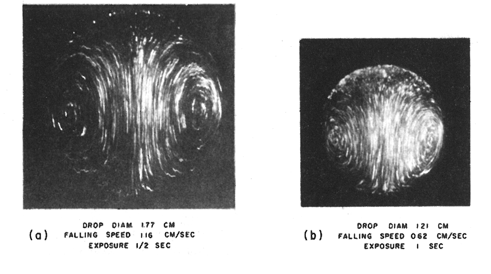
Figure 1: From the flow visualisation studies by Savic. Image showing a falling water drop in castor oil, with complete internal circulation, (a), and a stagnant cap, i.e. a downwards shift of the internal flow pattern, (b). Reproduced from Savic (1953) with permission from the National Research Council of Canada.

In this paper, we will extend the derivation by Chang and Berg (1985) of the analytical solution for the terminal velocity of a low $\operatorname{\mathit{R\kern-0.80002pte}}$ circular drop with an arbitrary surfactant (hence interfacial tension) distribution, taking here also the normal interfacial stresses into account. We show that this leads to a plethora of solutions, some of which are clearly unphysical (in the absence of an external energy input), such as a hovering drop. By appealing to the conservation of energy, we show that the physically admissible terminal velocities are bounded from below by the Stokes result for hard spheres, and from above by the Hadamard-Rybczynski result.

We proceed to supplement this with a simple model for the forces acting on surfactant molecules at the interface, giving an expression for the transition in terminal velocity between the two extremal values. This expression depends on the properties of the surfactant in question. From the theory we predict that for a given surfactant, the critical radius $R_{c}$ below which drops fall like hard spheres, should be proportional to the interfacial surfactant concentration. To confirm this prediction we determine the critical radii for the different bulk surfactant concentrations considered in the experiments performed by Griffith (1962). We demonstrate that these critical radii, when plotted against the bulk surfactant concentration, all collapse on a single Langmuir isotherm. Since the Langmuir isotherm relates the interfacial and the bulk surfactant concentration, this confirms the prediction by the present model, which we call the continuous-interface model.

We also discuss briefly the existing versions of the stagnant-cap model and to compare these with the model presented in this work. One should note that the straight-forward application of the stagnant-cap model gives rise to certain pecularities. As an example, consider Equation 7-270 on page 497 in the book by Leal (2007), which reads

$$\mbox{\boldmath$\nabla$}_{s}\cdot(\mathbf{u}_{s}\Gamma)\approx 0$$ (1)

where $\Gamma$ is the surfactant concentration. This equation follows from the assumption that the surfactant is insoluble, and that the interfacial Péclet number is $Pe_{s}=2R|\mathbf{u}_{s}|/D_{s}\gg 1$ where $\mathbf{u}_{s}$ is the velocity at the interface and $D_{s}$ is the interfacial diffusivity of the surfactant. From this, the classic stagnant cap result is obtained, namely that the part of the interface where the surfactant is found has $\mathbf{u}_{s}=0$ (this is the stagnant cap), and the rest of the interface has $\Gamma=0$. But if $\mathbf{u}_{s}=0$ in the stagnant cap region where the surfactant is located, then $Pe_{s}=0\not\gg 1$. Thus one is lead to consider what velocity is the appropriate to use in the surface Péclet number, if one is to keep the $Pe\gg 1$ assumption.

It should be noted that while the result obtained in this work for the interfacial tension distribution along the drop interface has the same functional form as the result obtained in the classic analysis e.g. by Levich (1962), unlike Levich, we do not assume the variation in surfactant concentration to be small, and since the present work avoids the use of a surfactant advection-diffusion equation on the interface (in contrast to previous approaches) we are able to obtain simultaneous analytical solutions to the flow and the interfacial tension distribution. This has been a major obstacle in previous work, as noted e.g. by Leal (2007):

It is not generally possible to obtain analytic solutions of the resulting problem because of the complexity of the surfactant transport phenomenon and the coupling between surfactant transport and fluid motion.

In closing, we argue that the present model could be more appropriate for interfacially active agents which are amphiphilic molecules, while the stagnant-cap model may be more appropriate for dispersed microscopic particulates which adsorb at the interface and thus modify the boundary conditions of the problem.

2 Theoretical results

2.1 Governing equations

The flow field $\mathbf{u}$ of an incompressible viscous Newtonian fluid is governed by the Navier-Stokes equations on the form

$$\mbox{\boldmath$\nabla$}\cdot\mathbf{u} =0\rm{,}$$ (2)

$$\frac{\partial\mathbf{u}}{\partial t}+(\mathbf{u}\cdot\mbox{\boldmath$\nabla$})\mathbf{u} =-\frac{\mbox{\boldmath$\nabla$}p}{\rho}+\frac{\mu}{\rho}\mbox{\boldmath$\nabla$}^{2}\mathbf{u}+\mathbf{f}_{\text{b}}\rm{.}$$ (3)

Here $p(\mathbf{x})$ is the pressure field and $\mathbf{f}_{\text{b}}$ is some external acceleration, such as gravity. As it stands, this system of equations is closed when fluid properties and initial and boundary conditions are given.

The system can be extended to two fluids by specifying an interface that separates fluid ₁ with properties $\rho_{1},\mu_{1}$ from fluid ₂ with properties $\rho_{2},\mu_{2}$, as well as two dynamic interfacial relations related to the interfacial tension $\sigma$. For the case of a drop or bubble we will mark the internal properties with ₁ and the external properties with ₂.

In order to have closure of Equation 3 with this extension, one also needs the following interfacial relations for two-phase flow:

$$\llbracket\mathbf{u}\rrbracket= \mathbf{0},$$ (4)

$$\mathbf{t}\cdot\llbracket\mathbf{T}\rrbracket\cdot\mathbf{n}= -\mathbf{t}\cdot\nabla\sigma,$$ (5)

$$\mathbf{n}\cdot\llbracket\mathbf{T}\rrbracket\cdot\mathbf{n}= \kappa\sigma.$$ (6)

Here the jump in a quantity across the interface is denoted by $\llbracket$-$\rrbracket$, $\mathbf{n}$ is the normal and $\mathbf{t}$ is a unit vector in the tangent plane to the interface, and $\mathbf{T}$ is the stress tensor. We choose the normal vector to point out from a drop, and the jump is then given by e.g. $\llbracket\mu\rrbracket=\mu_{2}-\mu_{1}$, i.e. the difference between the bulk and the drop value. In the case of a spherical droplet with zero velocity field, Equation 6 reduces to the Young-Laplace relation for the pressure difference across an interface ($\Delta p=2\sigma/R$). The Marangoni force comes in through Equation 5, and the functional form of the coefficient of interfacial tension along the drop interface, $\sigma$, is also needed for closure.

In this paper, the case of one spherical droplet falling in an unbounded domain will be considered. In this case, it is natural to introduce the following characteristic properties:

$$x^{\ast}=R,\quad u^{\ast}=U,\quad t^{\ast}=R/U,\quad p^{\ast}=\sigma/R,$$ (7)

giving the following non-dimensional Navier-Stokes equations:

$$\mbox{\boldmath$\nabla$}\cdot\mathbf{u} =0\rm{,}$$ (8)

$$\frac{\partial\mathbf{u}}{\partial t}+(\mathbf{u}\cdot\mbox{\boldmath$\nabla$})\mathbf{u} =\frac{1}{\operatorname{\mathit{R\kern-0.80002pte}}}\left[\mbox{\boldmath$\nabla$}^{2}\mathbf{u}+\frac{\operatorname{\mathit{R\kern-0.80002pte}}}{\operatorname{\mathit{W\kern-2.40005pte}}}\left(\operatorname{\mathit{E\kern-0.80002pto}}\,\mathbf{f}-\mbox{\boldmath$\nabla$}p\right)\right]\rm{.}$$ (9)

Here, $\operatorname{\mathit{R\kern-0.80002pte}}$ denotes the Reynolds number, $\operatorname{\mathit{W\kern-2.40005pte}}$ is the Weber number and $\operatorname{\mathit{E\kern-0.80002pto}}$ represents the Eötvös number. The Reynolds number is given by $\operatorname{\mathit{R\kern-0.80002pte}}=\rho_{2}UR/\mu_{2}$ as it is customary to use the continuous fluid properties in the dimensionless groups. This dimensionless number gives the ratio of inertial forces to viscous forces. The Weber number is given by $\operatorname{\mathit{W\kern-2.40005pte}}=\rho_{2}U^{2}R/\sigma$ and gives the ratio between inertial forces and interfacial tension forces. Lastly, the Eötvös number, $\operatorname{\mathit{E\kern-0.80002pto}}=\rho_{2}gR^{2}/\sigma$, gives the ratio between the body forces and the capillary forces.

In what follows, $\operatorname{\mathit{R\kern-0.80002pte}}$, $\operatorname{\mathit{W\kern-2.40005pte}}$ and $\operatorname{\mathit{E\kern-0.80002pto}}$ are all assumed to be small. The assumption of $\operatorname{\mathit{R\kern-0.80002pte}}\ll 1$ and of steady state flow simplifies the Navier-Stokes equation to the steady Stokes equation:

$$\mbox{\boldmath$\nabla$}^{2}\mathbf{u}+\frac{\operatorname{\mathit{R\kern-0.80002pte}}}{\operatorname{\mathit{W\kern-2.40005pte}}}\left(\operatorname{\mathit{E\kern-0.80002pto}}\,\mathbf{f}-\mbox{\boldmath$\nabla$}p\right)=\mathbf{0}\rm{.}$$ (10)

When $\operatorname{\mathit{W\kern-2.40005pte}}$ is small, $\operatorname{\mathit{W\kern-2.40005pte}}\ll 1$, the forces due to interfacial tension determine the shape of the interface through minimising the interfacial energy, which results in a spherical drop. As demonstrated by the Hadamard-Rybczynski result, the spherical falling drop is an exact solution to the Stokes equation. Furthermore, as demonstrated by Kojima et al. (1984) and in subsequent work (see Stone (1994, Chapter 6) for a review), perturbations away from the spherical shape for a drop falling at low $Re$ will either relax back toward the spherical shape, or form instabilities as elongated tails.

Lastly, the assumption of a small Eötvös number means that the body forces are small compared to the capillary forces, and hence will not alter the spherical shape of the droplet, but rather induce an acceleration on the droplet as a rigid body. In the case without surfactants, Taylor and Acrivos (1964) considered the deviation from a spherical shape at low $\operatorname{\mathit{E\kern-0.80002pto}}$ and found that this is $O(\operatorname{\mathit{R\kern-0.80002pte}}^{2})$, i.e. very small when $\operatorname{\mathit{R\kern-0.80002pte}}$ is small. In general, the assumption of a spherical drop is not a significant restriction, and so this assumption is ubiquitous in the literature on the falling drop at low $\operatorname{\mathit{R\kern-0.80002pte}}$ with surfactants (Savic, 1953; Levich, 1962; Griffith, 1962; Davis and Acrivos, 1966; Sadhal and Johnson, 1983; Leal, 2007).

2.2 Spherical droplet in a quiescent liquid

We will now consider a spherical droplet in a gravitational field surrounded by a quiescent liquid with which the droplet is immiscible. For a perfectly clean interface, the stationary solution is given by the Hadamard-Rybczynski solution. We proceed to let the interfacial tension vary along the interface and investigate the solutions obtained when accounting for the Marangoni force. We will follow in the steps of the analysis of Chang and Berg (1985), but we will also include the interfacial conditions for normal stresses. The appropriate boundary conditions are then given by Equations 4, 5 and 6.

We employ a spherical coordinate system $(r,\theta,\phi)$ fixed at the centre-of-mass of the droplet, with polar angle $\theta$ measured from the positive z-axis. For convenience we will at times refer to the axes of the Cartesian coordinate system, which has positive x-axis corresponding to $\theta=\pi/2,\phi=0$. This is illustrated in Figure 2.

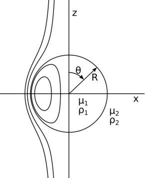
Figure 2: Illustration of coordinate system adopted, showing also the labelling of drop/bulk fluid properties.

The situation is cylindrically symmetric, so the azimuthal angle $\phi$ is redundant. The normal vectors in the $r$ and $\theta$ directions are denoted by $\mathbf{e}_{r}$ and $\mathbf{e}_{\theta}$, respectively. For a spherical drop, the normal (i.e. radial) velocity is zero at the interface, and the velocity far away from the droplet is given by

$$\mathbf{u}=U\cos\left(\theta\right)\mathbf{e}_{r}-U\sin\left(\theta\right)\mathbf{e}_{\theta},$$ (11)

where $U$ is the uniform velocity at infinity. The general solution for the stream functions outside and inside the droplet are found to be

$$\Psi_{2}= \sum_{n=2}^{\infty}\left(A_{n}r^{n}+B_{n}r^{1-n}+D_{n}r^{2+n}+E_{n}r^{3-n}\right)C^{-1/2}_{n}(\theta),$$ (12)

$$\Psi_{1}= \sum_{n=2}^{\infty}\left(F_{n}r^{n}+G_{n}r^{1-n}+H_{n}r^{2+n}+I_{n}r^{3-n}\right)C^{-1/2}_{n}(\theta),$$ (13)

where the velocity components are related to the stream function by

$$u_{r}=\frac{1}{r^{2}\sin\left(\theta\right)}\frac{\partial\Psi}{\partial\theta},$$ (14)

$$u_{\theta}=-\frac{1}{r\sin\left(\theta\right)}\frac{\partial\Psi}{\partial r}.$$ (15)

Requiring a uniform velocity at infinity gives

$$A_{2} =-U,$$ (16)

$$A_{n} =0\quad\forall n\geq 3,$$ (17)

$$D_{n} =0\quad\forall n\geq 2,$$ (18)

and the assumption that the velocity is bounded at the origin gives

$$G_{n} =0\quad\forall n\geq 2,$$ (19)

$$I_{n} =0\quad\forall n\geq 2.$$ (20)

The vanishing normal velocity at the interface ($r=R$) gives

$$B_{2} =R^{3}U-R^{2}E_{2},$$ (21)

$$B_{n} =-R^{2}E_{n}\quad\forall n\geq 3,$$ (22)

$$H_{n} =-\frac{F_{n}}{R^{2}}\quad\forall n\geq 2.$$ (23)

The final kinematic boundary condition, the continuity of the velocity field across the interface, gives

$$E_{2} =\frac{3}{2}RU-RF_{2},$$ (24)

$$E_{n} =-R^{2n-3}F_{n}\quad\forall n\geq 3.$$ (25)

Both stream functions can now be expressed through one common set of coefficients

$$\Psi_{2}= \left(-Ur^{2}-\left(\frac{R^{3}}{2}U-R^{3}F_{2}\right)\frac{1}{r}+\left(\frac{3}{2}RU-RF_{2}\right)r\right)C^{-1/2}_{2}$$

$$+ \sum_{n=3}^{\infty}\left(\frac{R^{2n-1}}{r^{n-1}}-\frac{R^{2n-3}}{r^{n-3}}\right)F_{n}C^{-1/2}_{n},$$ (26)

$$\Psi_{1}= \sum_{n=2}^{\infty}\left(r^{n}-\frac{r^{n+2}}{R^{2}}\right)F_{n}C^{-1/2}_{n},$$ (27)

where $R$ is the radius of the droplet.

The dynamic interfacial conditions will now be used to determine the last coefficient and the interfacial tension as a function of the polar angle. Since the Legendre polynomials form a complete orthonormal basis for any periodic function, we may write

$$\sigma=\sum_{n=0}^{\infty}\sigma_{n}\text{P}_{n}\left(\eta\right),$$ (28)

where $\eta=\cos\left(\theta\right)$ and $\text{P}_{n}$ is the $n$’th Legendre polynomial. The normal stress condition (Equation 6) in spherical coordinates can be written as

$$\llbracket-p\rrbracket+2\llbracket\mu\frac{\partial}{\partial r}\left(\frac{1}{r^{2}}\frac{\partial\Psi}{\partial\eta}\right)\rrbracket=\frac{2}{R}\sigma,$$ (29)

giving the following relations between $F_{n}$ and $\sigma_{n}$

$$\sigma_{0}= \frac{R}{2}\left(p_{01}-p_{02}\right),$$ (30)

$$\sigma_{1}= \frac{3}{4}\mu_{2}U-\frac{1}{2}\left(\rho_{1}-\rho_{2}\right)gR^{2}+\left(\frac{3}{2}\mu_{2}+3\mu_{1}\right)F_{2},$$ (31)

$$\sigma_{n}= 6R^{n-2}\left(\frac{\mu_{1}}{2\left(n-1\right)}+\frac{\mu_{2}}{2n}\right)F_{n+1}\quad\forall n\geq 2.$$ (32)

Similarly, the shear stress condition (Equation 5), containing the Marangoni force, gives the relations

$$\sigma_{1}= -\frac{3}{2}\mu_{2}U+3\left(\mu_{2}+\mu_{1}\right)F_{2},$$ (33)

$$\sigma_{n}= 2R^{n-2}\frac{2n-1}{n\left(n+1\right)-6}\left(\mu_{1}+\mu_{2}\right)F_{n+1}\quad\forall n\geq 2.$$ (34)

The simultaneous solution to Equations 30, 31 and 32 and Equations 33–34 is given by

$$\sigma_{0}= \frac{R}{2}\left(p_{01}-p_{02}\right),$$ (35)

$$\sigma_{1}= \frac{9}{2}\mu_{1}\left(U-U_{\text{HS}}\right)+\frac{1}{2}\mu_{2}\left(6U-9U_{\text{HS}}\right),$$ (36)

$$\sigma_{n}= 0\quad\forall n\geq 2,$$ (37)

$$F_{2}= \frac{3}{2}\left(U-U_{\text{HS}}\right),$$ (38)

$$F_{n}= 0\quad\forall n\geq 3,$$ (39)

where $p_{0i}$ is the reference pressure in the respective phases and

$$U_{\text{HS}}=\frac{2\Delta\rho|\mathbf{g}|R^{2}}{9\mu_{2}},$$ (40)

where $\Delta\rho=(\rho_{1}-\rho_{2})$, is the Stokes result for the terminal velocity of a hard sphere. By insertion, one finds that the expression for $\sigma_{1}$ is zero if $U$ is replaced by the solution given by Hadamard and Rybczynski, which is consistent with the assumption of two clean fluids.

The resulting expressions for the stream functions can now be given by

$$\Psi_{1}\left(r,\theta\right) =\frac{3}{4}\left(U-U_{\text{HS}}\right)\left(r^{2}-\frac{r^{4}}{R^{2}}\right)\sin^{2}\left(\theta\right),$$ (41)

$$\Psi_{2}\left(r,\theta\right) =\frac{1}{2}\left(-Ur^{2}+\frac{3}{2}U_{\text{HS}}Rr+\left(U-\frac{3}{2}U_{\text{HS}}\right)\frac{R^{3}}{r}\right)\sin^{2}\left(\theta\right).$$ (42)

One may also notice that the internal stream function is identically equal to zero if $U$ is replaced by $U_{\text{HS}}$. This shows that if the droplet is falling with the same velocity as a hard sphere, the Marangoni forces will balance the shear forces from the external fluid, resulting in a uniform velocity inside the droplet equal to the droplet velocity.

The above analysis does not give any restrictions on the velocity of the droplet, other than the demand of keeping the Reynolds number low. An exotic case would be that of a hovering droplet, meaning that the Marangoni forces balance the forces induced by gravity. In the absence of an energy input e.g. from a temperature gradient (Young et al., 1959) or from an asymmetric release of surfactants (Masoud and Stone, 2014), both of which are interesting systems in their own right, a hovering drop will clearly violate the conservation of energy.

The expression for the stream function shows that there is a non-zero velocity field in this case. This is obvious from the fact that in the presence of Marangoni forces, the viscous stress tensor cannot be zero both inside and outside the droplet, and hence there must be gradients in the velocity field. In Figure 3 we plot (a) the vectors of the velocity field around the hovering drop and (b) the decay of the velocity field far away from the drop. This case corresponds of course to $U=0$, so the coordinate systems of the drop and the laboratory coincide.

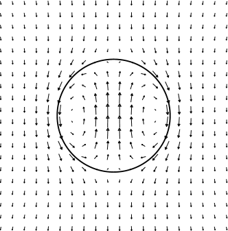
(a) The vector field $\mathbf{u}$ around the hovering droplet.

(b) Signed magnitude of the velocity along the z- and x-axis, $\theta=0$ and $\theta=\pi/2$ respectively.

Figure 3: The velocity field in the case of a hovering drop (terminal velocity equal to zero). In (a) the vector field is shown close to the drop. In (b) line plots of the velocity along the polar (z-axis) and the azimuthal (x-axis) directions. It is seen that the velocity field decays to zero far away from the drop. Note that the sharp kink in (b) is caused by the drop interface.

To proceed, one may consider the energy balance in this system, in order to pick physically acceptable solutions. The energy equation for creeping flow can be obtained from the Navier-Stokes equations as:

$$\dot{\text{e}}_{\text{K}}= \frac{\partial}{\partial t}\left(\rho\frac{u^{2}}{2}\right)=\mathbf{u}\cdot\left(\mbox{\boldmath$\nabla$}\cdot\mathbf{T}\right)+\rho\mathbf{u}\cdot\mathbf{f}_{\text{b}}+\mathbf{u}\cdot\mathbf{f}_{\text{I}}(r,l)\delta\left(\mathbf{x}-\mathbf{x}_{\text{I}}(r,l)\right)\,\text{d}r\,\text{d}l$$ (43)

$$= \mbox{\boldmath$\nabla$}\cdot\left(\mathbf{u}\cdot\mathbf{T}\right)-\mathbf{T}\colon\mbox{\boldmath$\nabla$}\mathbf{u}+\rho\mathbf{u}\cdot\mathbf{f}_{\text{b}}+\mathbf{u}\cdot\int_{\Gamma}\mathbf{f}_{\text{I}}(r,l)\delta\left(\mathbf{x}-\mathbf{x}_{\text{I}}(r,l)\right)\,\text{d}r\,\text{d}l,$$ (44)

where $\delta(\mathbf{x}-\mathbf{x}_{\text{I}})$ is a Dirac delta-function which is singular at the interface and $r$ and $l$ is the parametrisation of the interface. The first term on the right of Equation 44 is the energy flux passing through a fluid interface (or any finite volume in the general case) and the second term is the energy dissipation in a fluid element. The third term is the energy provided by the body force term, while the last term is the energy dissipated in the interface due to the action of the surfactants. For the sake of brevity we will refer to this dissipation as “energy consumption” (or “energy production” in the opposite case), even though energy can of course not be consumed or produced.

Figure 4: The integration domain $\Omega$ of thickness $\epsilon$ around the droplet interface $\Gamma$.

We will now look at the energy balance of the interface itself. This is achieved by integrating Equation 44 over a volume just enclosing the interface (see Figure 4):

$$0=\int_{\Omega}\mbox{\boldmath$\nabla$}\cdot\left(\mathbf{u}\cdot\mathbf{T}\right)\,\text{d}\mathbf{x}-\int_{\Omega}\mathbf{T}\colon\mbox{\boldmath$\nabla$}\mathbf{u}\,\text{d}\mathbf{x}+\int_{\Omega}\rho\mathbf{u}\cdot\mathbf{f}_{\text{b}}\,\text{d}\mathbf{x}+\int_{\Omega}\mathbf{u}\cdot\int_{\Gamma}\mathbf{f}_{\text{I}}\delta\left(\mathbf{x}-\mathbf{x}_{\text{I}}\right)\,\text{d}S\,\text{d}\mathbf{x}$$ (45)

After applying Gauss’ theorem and letting $\epsilon$ approach zero (following Hansen (2005)), one obtains

$$0=-\underbrace{\oint\mathbf{u}_{2}\cdot\mathbf{T}_{2}\cdot\mathbf{n}\,\text{d}S}_{E_{1}}+\underbrace{\oint\mathbf{u}_{1}\cdot\mathbf{T}_{1}\cdot\mathbf{n}\,\text{d}S}_{E_{2}}+\underbrace{\oint\left(\mathbf{u}_{1}\cdot\mathbf{t}\right)\left(\mathbf{t}\cdot\mbox{\boldmath$\nabla$}\sigma\right)\,\text{d}S}_{E_{3}},$$ (46)

where we have labelled the terms for reference in Figure 5, and where

$$\mathbf{u}\cdot\mathbf{T}\cdot\mathbf{n}=-pu_{r}+\mu\left(2u_{r}\frac{\partial u_{r}}{\partial r}+u_{\theta}\frac{\partial u_{\theta}}{\partial r}-\frac{u_{\theta}^{2}}{r}+\frac{u_{\theta}}{r}\frac{\partial u_{r}}{\partial r}\right)$$ (47)

in spherical coordinates. We have also used an inward pointing normal vector so that energy flux into the droplet is positive. Since there is no net movement of the drop, the integration over the droplet of the body force term in Equation 44 will be zero. Thus Equation 46 shows that the energy consumption in the interface together with the energy dissipation in the droplet at stationary conditions must equal the energy flux into the droplet interface from the surrounding fluid side.

The three terms in Equation 46 are plotted individually in Figure 5. The figure shows that there is an interval where the interface is consuming energy to keep the constant velocity. Since we are not providing external energy to the interface, this is the only allowed velocity interval. By setting the third term in Equation 46 to zero, a second order equation for the velocity gives:

$$U=U_{\text{HS}}\quad\vee\quad U=3\frac{\mu_{1}+\mu_{2}}{3\mu_{1}+2\mu_{2}}U_{\text{HS}},$$ (48)

as the bounding interval. So, the permissible solutions for a viscous sphere falling at steady state in a gravitational field surrounded by a quiescent liquid under the influence of Marangoni forces are bounded by the Stokes solution for the hard sphere and the Hadamard-Rybczynski solution for clean liquids. Note again the contrast here with the stagnant-cap model, where these two bounds are assumed a priori.

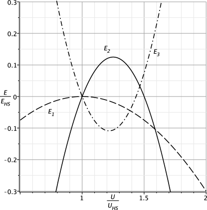
Figure 5: Energy consumption for the falling droplet. Negative values indicate energy consumption, while positive values are energy production. The term $E_{3}$ is the third term on the right-hand side of Equation 46, viz. $E_{3}=E_{1}-E_{2}$, and we see clearly that the interval in which the interface consumes energy is bounded by the Stokes and the Hadamard-Rybczynski terminal velocities, cf. Equation 48. Outside these limits, the interface produces energy, which is unphysical.

To compare this result directly to the stagnant-cap model, one may consider the terminal velocity of the droplet given as a function of the interfacial tension,

$$U= \frac{3\left(\mu_{1}+\mu_{2}\right)}{3\mu_{1}+2\mu_{2}}U_{\text{HS}}-\frac{2\sigma_{1}}{9\mu_{1}+6\mu_{2}}$$ (49)

$$= U_{\text{HR}}-\frac{2\sigma_{1}}{9\mu_{1}+6\mu_{2}},$$ (50)

where the reader is reminded that the interfacial tension is $\sigma=\sigma_{0}-\sigma_{1}\cos\left(\theta\right)$ and that $U_{\text{HR}}$ is the Hadamard-Rybczynski velocity. This gives the following expression for the drag force on the droplet:

$$\text{F}_{\text{D}}=\frac{4\pi\mu_{2}UR}{1+\beta}\left[\frac{3}{2}\beta+1+\frac{\sigma_{1}}{3\mu_{2}U}\right],$$ (51)

where $\beta$ is the ratio of the inner and outer fluid viscosity. In comparison, the drag force obtained with the stagnant cap model can be written as

$$\text{F}_{\text{D}}=\frac{4\pi\mu_{2}UR}{1+\beta}\left[\frac{3}{2}\beta+1+f_{1}\left(f_{2}^{-1}\left(\frac{1+\beta}{\mu_{2}U}\sigma_{\Delta}\right)\right)\right],$$ (52)

where $\sigma_{\Delta}$ is the difference between the maximum and minimum value of interfacial tension as defined in Sadhal and Johnson (1983), and $f_{1}$ and $f_{2}$ are trigonometric functions of the cap angle (Hatanaka et al., 1988). Davis and Acrivos (1966) assumed that $\sigma_{\Delta}$ was limited by a constant value $\Pi^{*}$, making the argument in $f_{2}^{-1}$ approach zero when the droplet radius (hence the terminal velocity) increases. One then obtains the desired behaviour with the drag force approaching that for clean droplets.

2.3 The continuous-interface model

Proceeding from this result, we will derive a mechanical interface model which links the interfacial concentration of surfactants to the coefficient of interfacial tension. To achieve this we will use arguments from molecular considerations, and link the dynamic equations directly to the Marangoni force.

It is assumed that the surfactant molecules are subjected to a force field, $\mathbf{f}$, and that their action on each other due to thermal fluctuations is governed by a Wiener process, i.e. a force given by $\lambda\mathbf{F}_{s}$ where $\lambda$ is a scaling parameter for the normalised stochastic Wiener function $\mathbf{F}_{s}$. It is customary (Giona et al., 2004) to model the fluid friction on each molecule by a Stokesian force term, $\mathbf{f}=\psi\mathbf{u}$, where $\psi$ is a friction constant and $\mathbf{u}$ is the velocity of the species surrounding the molecule in question. This leads to Brownian motion, whose stochastic behaviour in the diffusion-controlled regime is governed by the Langevin equation (Giona et al., 2004)

$$\frac{d\mathbf{x}}{dt}=-\frac{\mathbf{f}}{\psi}-\frac{\sigma}{\psi}\mathbf{F}_{s}.$$ (53)

This equation corresponds to a Fokker-Plank equation which is the macroscopic advection diffusion equation (Castiglione et al., 1999),

$$\frac{\partial\Gamma}{\partial t}+\mbox{\boldmath$\nabla$}\cdot\mathbf{j}=D_{s}\mbox{\boldmath$\nabla$}^{2}{\Gamma},$$ (54)

where $\Gamma$ is the interfacial concentration of the species in question, $D_{s}=1/2(\sigma/\psi)^{2}$ is the interfacial diffusion coefficient, and $\mathbf{j}=\mathbf{f}/\psi\Gamma$ is the flux. This advection-diffusion equation is the typical starting point for modelling the transport of surfactants on the droplet interface (Levich, 1962; Leal, 2007).

In the situation where surfactants retard the velocity of the droplet to that of a hard sphere, the advection-diffusion equation dictates that the only possible surfactant concentration profile is a constant one. This conclusion is the basis for the stagnant cap model, namely that one section of the droplet surface has a constant concentration of surfactants, and the remainder is completely empty of surfactants. This means that the coefficient of surface tension abruptly goes from one constant value on the cap section to another (generally higher) constant value on the rest of the droplet. A surfactant concentration profile being piecewise constant is hard to relate to the Marangoni force (Sadhal and Johnson, 1983), which depends on a gradient in the interfacial tension.

In order to relate the Marangoni force to the retardation of covered droplets, we are forced to alter the advection-diffusion equation approach used e.g. by Levich (1962). Alternatively, as is done here, we may consider a force balance on the surfactant layer, viz.

$$\Gamma\frac{d\mathbf{u}}{dt}=\mbox{\boldmath$\nabla$}\cdot\mathbf{T}_{\text{s}}+\mathbf{f}_{\text{M}},$$ (55)

where $\Gamma$ is the concentration of surfactants, $\mathbf{T}_{\text{s}}$ is the two-dimensional surface stress tensor and $\mathbf{f}_{\text{M}}$ is a body force affecting the surface layer, namely the Marangoni force. It should be noted that we now treat the surfactants as a two-dimensional continuum on the interface of the droplet. Assuming steady-state and inserting the expression for the Marangoni force, the force balance becomes

$$0=\mathbf{t}\cdot\mbox{\boldmath$\nabla$}\cdot\mathbf{T}_{\text{s}}-\mathbf{t}\cdot\mbox{\boldmath$\nabla$}\sigma.$$ (56)

We now assume that the surfactants form an inviscid continuum, i.e. we neglect here surface (shear and dilatational) viscosities, so the stress tensor reduces to only a pressure term, $\mathbf{T}_{s}=-p_{\text{I}}\mathbf{I}$, giving the following relation between the pressure in the interfacial layer and the coefficient of surface tension:

$$p_{\text{I}}=\alpha-\beta\sigma,$$ (57)

where $\alpha$ and $\beta$ are constants to be determined. The pressure in the interface is related to the concentration of surfactants through a constitutive relation such as the Langmuir-Blodgett equation of state (see e.g. Langmuir, 1917). Neglecting the surface viscosities is a reasonable approximation here, as it is a weaker effect than e.g. surface tension and the Marangoni force, but we note that interesting phenomena do arise from the surface viscosity (Agrawal and Wasan, 1979) and may consider the extension to include this in future work.

The aim of the present approach is to give an alternative model to the stagnant-cap model. The new model should have some predictive power, explaining some results obtained in experiments; in particular we will consider the paper by Griffith (1962). In that paper, relatively low concentrations of surfactant are used, starting from almost pure fluids. In this case, we will assume that the concentration of surfactants in the interfacial layer is small, and therefore use a linear approximation to the Langmuir-Blodgett equation of state, giving a linear relation between the interfacial tension and the concentration of surfactants

$$\Gamma(\theta) =C-\frac{\sigma}{k}$$ (58)

$$=C-\frac{\sigma_{0}}{k}+\frac{\sigma_{1}}{k}\cos(\theta)$$ (59)

$$=\Gamma_{\text{avg}}+\frac{\sigma_{1}}{k}\cos\left(\theta\right),$$ (60)

where the last line is obtained by integrating $\Gamma(\theta)$ over the sphere and setting the result equal to $4\pi R^{2}\Gamma_{\text{avg}}$.

It is readily apparent from Equation 60 that $\Gamma$ as a function of $\theta$ is symmetric about $\Gamma_{\text{avg}}$, and that the minimum is given by $\Gamma_{\text{avg}}-\sigma_{1}/k$, which implies that

$$\sigma_{1}\leq k\Gamma_{\text{avg}}.$$ (61)

Positing that there exists a maximum value for the repulsive force between the surfactants, the surfactant would be released from the interface and dissolve into the bulk phase, Equation 60 shows that $\Gamma$ must be less than some maximum value $\Gamma_{\infty}$. $\Gamma_{\infty}$ is known as the maximum packing concentration in the surfactant literature. Inserting $\Gamma_{\infty}\geq\Gamma$ into Equation 60 one obtains

$$\Gamma_{\text{avg}}\leq\Gamma_{\infty}-\sigma_{1}/k,$$ (62)

giving

$$\sigma_{1}\leq\frac{k\Gamma_{\infty}}{2}.$$ (63)

In arriving at these expressions, it was implicitly assumed that there is no limit to the forces each surfactant molecule can absorb from the surrounding liquids. In reality, the surfactant molecules will bend and twist if they are subjected to large stresses. Taking this into account, i.e. requiring that each molecule can at most absorb a force of magnitude $F_{\infty}$, one obtains a restriction on the Marangoni shear stress $\tau=\sigma_{1}\sin(\theta)/R$, namely $\tau/\Gamma\leq F_{\infty}$. In addition to this comes the requirement that $\Gamma\leq\Gamma_{\infty}$ as discussed previously.

Writing it out in full, this expression for the maximum interfacial shear stress is

$$\max_{\theta}\frac{\tau}{\Gamma(\theta)}=\max_{\theta} \frac{\frac{1}{R}\sigma_{1}\sin(\theta)}{\Gamma_{\text{avg}}+\frac{\sigma_{1}}{k}\cos(\theta)}\leq F_{\infty},$$ (64)

or equivalently

$$\max_{\theta}\,\sigma_{1}\left(\frac{\sin(\theta)}{R}-\frac{F_{\infty}}{k}\cos(\theta)\right)\leq F_{\infty}\Gamma_{\text{avg}},$$ (65)

giving a restriction on the rate of change of the interfacial tension,

$$\sigma_{1}\leq \frac{k\Gamma_{\text{avg}}}{\sqrt{1+\left(\frac{k}{F_{\infty}R}\right)^{2}}}\leq k\Gamma_{\text{avg}},$$ (66)

which upon insertion of Equation 62 yields

$$\sigma_{1}\leq\frac{k\Gamma_{\infty}}{1+\sqrt{1+\left(\frac{k}{F_{\infty}R}\right)^{2}}}\leq\frac{k\Gamma_{\infty}}{2}.$$ (67)

Using Equation 49 to eliminate $\sigma_{1}$ from Equation 66, one obtains now an expression for the lowest terminal velocity allowed for a drop of radius $R$. Normalising this by the terminal velocity of a hard sphere, $\chi=U/U_{\text{HS}}$, gives

$$\chi\geq\frac{3\left(\mu_{1}+\mu_{2}\right)}{3\mu_{1}+2\mu_{2}}- \frac{2}{9\mu_{1}+6\mu_{2}}\frac{k\Gamma_{\text{avg}}}{U_{\text{HS}}\sqrt{1+\left(\frac{k}{F_{\infty}R}\right)^{2}}}.$$ (68)

At this point it is convenient to introduce the viscosity ratio $\beta=\mu_{1}/\mu_{2}$, as well as the quantity $R_{c}=k/F_{\infty}$. This critical radius $R_{c}$ is the largest droplet radius such that the forces from the surfactants on the liquid are large enough to retard the droplet to the Stokes terminal velocity ($\chi=1$). We denote the drop radius normalised by the critical radius as $x=R/R_{c}$. Using the fact that this expression should become 1 at $x=1$, i.e. that drops with the critical radius fall like hard spheres, we obtain $\Gamma_{\text{avg}}/R_{c}=\sqrt{2}\Delta\rho g/3F_{\infty}$, and the previous equation simplifies to

$$\chi\geq\frac{3\left(\beta+1\right)}{3\beta+2}- \frac{\sqrt{2}}{3\beta+2}\frac{x^{-2}}{\sqrt{1+x^{-2}}}.$$ (69)

Notice that in the expression for $\Gamma_{\text{avg}}/R_{c}$ preceding this equation, the maximum force a surfactant molecule can absorb, $F_{\infty}$, is a material constant for the surfactant. This means that for a given surfactant, the average interfacial concentration is directly proportional to the critical radius. Thus, in low surfactant-concentration experiments, one may use the critical radius as a measure of equilibrium interfacial concentration of surfactants, $\Gamma_{\text{avg}}$. The reader is reminded that $\Gamma_{\text{avg}}$ can be related to the bulk concentration of surfactants, $C$, by a Langmuir isotherm

$$\Gamma_{\text{avg}}=\Gamma_{\infty}\frac{aC}{1+aC}$$ (70)

where $a$ is a constant.

Recalling the proof in Section 2.2 that a drop cannot fall slower than a hard sphere of equal radius, since this violates the conservation of energy, we obtain the final expression for the relative velocity $\chi$ as

$$\chi(x)\geq\begin{cases}1&\text{if}\;x\leq 1\rm{,}\\ \frac{3\left(\beta+1\right)}{3\beta+2}-\frac{\sqrt{2}}{3\beta+2}\frac{x^{-2}}{\sqrt{1+x^{-2}}}&\text{if}\;x>1.\end{cases}$$ (71)

Notice that this expression is continuous at $x=1$, but the derivative is discontinuous at this point, cf. Figure 7. Notice also that when $R\gg R_{c}$, i.e. $x^{-2}\ll 1$, the expression for $x>1$ approaches the Hadamard-Rybczynski result. Thus the inequality must be replaced by equality in the $x\gg 1$ limit. In the $x\to 1$ limit, equality is also required since it is observed that the drops fall like hard spheres. The simplest expression which is correct in both these limits is obtained by replacing the inequality with equality for the entire expression, viz.

$$\chi(x)=\begin{cases}1&\text{if}\;x\leq 1\rm{,}\\ \frac{3\left(\beta+1\right)}{3\beta+2}-\frac{\sqrt{2}}{3\beta+2}\frac{x^{-2}}{\sqrt{1+x^{-2}}}&\text{if}\;x>1.\end{cases}$$ (72)

This is the prediction of the continuous-interface model for the transition in terminal velocity as a function of drop radius.

3 Discussion

In 1953, Savic (1953) introduced the stagnant cap model (SCM) as an explanation of the experimental results obtained by Bond (1927); Bond and Newton (1928). The SCM incorporates the effect of surfactants through a rigid cap where a no-slip boundary condition is used. It is obvious that this will lead to a terminal velocity of droplets bounded by the Stokes velocity and the Hadamard-Rybczynski velocity. In later works several iterations of the SCM have been proposed(Griffith, 1962; Davis and Acrivos, 1966; Harper, 1973; Sadhal and Johnson, 1983), and presently two different versions exist, namely the model proposed by Griffith (1962) and the model proposed by Davis and Acrivos (1966). The Griffith approach is based on calculating the cap angle from a criterion based on the average interfacial pressure difference, while Davis and Acrivos employ a local criterion based on the capillary tension and the interfacial shear forces.

Hatanaka et al. (1988) give a review of the experiments performed by Bond and Newton (1928) and Griffith (1962) and compare the two versions of the SCM with the experimental results. Hatanaka et al. show that the model of Davis and Acrivos gives better agreement with the experiments performed by Bond and Newton (1928), while the Griffith model gives better agreement with the experimental results performed by Griffith himself. It appears that the difference between the experimental results by Griffith and those of Bond and Newton is too large to be governed by the same mechanism. Note here that while the experiments due to Bond and Newton (1928) use fluids which are assumed to be pure, in the experiments by Griffith (1962) a surfactant is deliberately added at known bulk concentrations. In general, one considers the experiments performed by Griffith (1962) to be more reliable, since the experimental setup there is better controlled, taking advantage of developments in our understanding of chemistry and fluid mechanics, as well as developments in experimental equipment, not available at the time of Bond and Newton (1928).

Figure 6 shows one set of experiments performed by Griffith (1962), extracted from Figure 9 in his work. The figure shows the results from an experiment with drops of ethylene glycol with Aerosol 61 surfactant falling in a reservoir of a mineral oil, using different concentrations of surfactant. The results are plotted as the relative velocity $\chi=U/U_{HS}$ versus the drop radius. Notice that the base fluids employed by Griffith are not free of surface active agents, indicated by the results without any added surfactant showing the same trend of approaching the hard sphere terminal velocity as the radius decreases.

Figure 6: Droplet terminal velocities for different drop sizes and at different surfactants concentrations (Griffith (1962, Fig. 9)). The concentration is given in $\,\mathrm{kg/m^{3}}$ and the highest concentration corresponds to $35.4\,\mathrm{ppm}$.

By fitting Equation 72 to these data points, we may calculate the critical radius $R_{c}$ below which $\chi=1$ in the experiments performed by Griffith. This is shown in Figure 7, where the obtained values of $R_{c}$ for each of the five concentrations is shown in the legend. Note that in theory, if perfectly pure fluids were used, $R_{c}\to 0$ as $C\to 0$. This is not the case for these experiments.

Figure 7: Nonlinear curve fit of Equation 72 to the raw data by Griffith (1962).

As outlined in the previous section, the proposed continuous-interface model predicts that the critical radius is directly proportional to the interfacial surfactant concentration, which can again be related to the bulk concentration through the Langmuir isotherm Equation 70. This means the critical radius is also related to the bulk concentration via a Langmuir isotherm, i.e. we can write $R_{c}=R_{c}(C)$. Notice, however, that the isotherm must be modified to account for the fact that surfactants are still present in the system at $C=0$, i.e. $R_{c}(C=0)\neq 0$. By replacing the concentration in Equation 70 with $C^{\prime}=C+C_{\text{base}}$, we obtain an isotherm with two unknown parameters, $a$ and $C_{\text{base}}$. Fitting this to the experimental data, as shown in Figure 8, it is seen that the critical radii all collapse to the obtained Langmuir isotherm. This confirms the prediction made by the proposed continuous-interface model.

Figure 8: $R_{c}$ obtained from the fitting of Equation 72 to the experimental data, plotted against bulk surfactant concentration, together with a Langmuir isotherm fitted to these points.

To complete this discussion, we wish to point out that the stagnant cap model is likely a good model when the surface-active agents interact like hard particles. To see this, consider the explanation of the stagnant cap model in terms of the Marangoni force, as attempted by Sadhal and Johnson (1983). If the Marangoni stress balance is valid, then arguably the normal stress balance should also be satisfied. In the SCM, none of the above stress balances are used as boundary conditions. It is then only possible (given the uniqueness of solutions to the Stokes equation) to satisfy both stress balances if one of them can be written in terms of the boundary conditions used. This is obviously not possible, and hence the normal stress balance cannot be satisfied.

It is therefore natural to conclude that the SCM may be applicable in situations where interfacially active components interact like particles and form a solid cap. In the continuous-interface model presented here, both stress balances are used in the boundary conditions and therefore, in contrast to the SCM, it applies when the interfacially active components are amphiphilic molecules which produce a Marangoni force.

4 Concluding remarks

In this paper we have derived the exact solution to the flow inside and around a circular drop falling at low Reynolds number, with an arbitrarily varying interfacial tension. By avoiding the use of a surfactant advection-diffusion equation at the interface, we are able to obtain analytical solutions to the flow, which has not been possible in previous works. We demonstrate that when all the interfacial stress conditions are taken into account, one obtains a range of simultaneous solutions for the variation in interfacial tension and for the flow field, including exotic solutions such as the hovering drop. By appealing to conservation of energy, we restrict the allowed interval of solutions, and show that the terminal velocity of a falling drop must lie between the clean drop (Hadamard-Rybczynski) and the rigid sphere (Stokes) results.

To proceed with this approach, we propose a new model for how surfactants behave at the interface of a falling drop. Previous work has assumed the existence of a stagnant cap of surfactants on the top of a falling drop. In the present model we do not impose a specific surfactant distribution, but we introduce a simple model, called the continuous-interface model, which takes into account the force balance for surfactant molecules at the interface. It is demonstrated that the model gives a transition in terminal velocity as a function of drop radius that is consistent with experimental results. Moreover, by fitting the model to experimental results, we extract values for the critical radius as a function of bulk surfactant concentration. The model predicts that these should be related by a Langmuir isotherm, and indeed this is found to be true. We postulate that our model is more reasonable for fluid-like surfactant molecules, while the stagnant cap model may be appropriate for colloidal particles acting as surfactants. Future work may attempt to identify this difference experimentally.

Ending on a historical note, we have read with interest the relatively recent paper by Hager (2012) about the life and work of Wilfrid Noel Bond, who, amongst other achievements, was the first person to observe and discuss the transition in terminal velocity that we aim to explain with our model. Bond’s untimely demise was surely a great loss not only for his family, but also for the field of fluid mechanics research.

The authors are grateful for stimulating discussions on these matters with Dr. Svend Tollak Munkejord and Professor Bernhard Müller, as well as for the comments of the anonymous referees which helped improve this paper. This work was funded by the project Fundamental understanding of electrocoalescence in heavy crude oils coordinated by SINTEF Energy Research. The authors acknowledge the support from the Petromaks programme of the Research Council of Norway (206976), Petrobras, Statoil and Sulzer Chemtech.

References

- Agrawal and Wasan (1979) S. Agrawal and D. Wasan. The effect of interfacial viscosities on the motion of drops and bubbles. The Chemical Engineering Journal, 18(2):215 – 223, 1979. ISSN 0300-9467. doi: 10.1016/0300-9467(79)80043-X.
- Bond (1927) W. N. Bond. LXXXII. Bubbles and drops and Stokes’ law. Phil. Mag., 4(24):889–898, 1927.
- Bond and Newton (1928) W. N. Bond and D. A. Newton. LXXXII. Bubbles and drops and Stokes’ law. (Paper 2). Phil. Mag., 5(30):794–800, 1928.
- Castiglione et al. (1999) P. Castiglione, A. Mazzino, P. Muratore-Ginanneschi, and A. Vulpiani. On strong anomalous diffusion. Physica D: Nonlinear Phenomena, 134(1):75 – 93, 1999. doi: 10.1016/S0167-2789(99)00031-7.
- Chang and Berg (1985) L. S. Chang and J. C. Berg. The effect of interfacial tension gradients on the flow structure of single drops or bubbles translating in an electric field. AIChE J., 31(4):551–557, 1985.
- Clift et al. (1978) R. Clift, J. R. Grace, and M. E. Weber. Bubbles, drops and particles. Academic Press, 1978.
- Davis and Acrivos (1966) R. E. Davis and A. Acrivos. The influence of surfactants on the creeping motion of bubbles. Chem. Eng. Sci., 21(8):681 – 685, 1966.
- Edge and Grant (1972) R. M. Edge and C. D. Grant. The motion of drops in water contaminated with a surface-active agent. Chem. Eng. Sci., 27(9):1709 – 1721, 1972.
- Frumkin and Bagotskaya (1947) A. Frumkin and I. Bagotskaya. Unknown title (in Russian), cited in Levich: “Physicochemical Hydrodynamics”. Comptes Rendus de l’Académie des Sciences de l’URSS, 55(131), 1947.
- Frumkin and Levich (1947) A. Frumkin and V. Levich. On surfactants and interfacial motion. Zh. Fiz. Khim, 21:1183–1204, 1947.
- Giona et al. (2004) M. Giona, S. Cerbelli, and V. Vitacolonna. Universality and imaginary potentials in advection–diffusion equations in closed flows. Journal of Fluid Mechanics, 513:221–237, 8 2004. doi: 10.1017/S002211200400984X.
- Griffith (1962) R. Griffith. The effect of surfactants on the terminal velocity of drops and bubbles. Chem. Eng. Sci., 17(12):1057 – 1070, 1962.
- Hadamard (1911) J. Hadamard. Mouvement permanent lent d’une sphère liquide et visqueuse dans un liquide visqueux. Comp. Rend. Acad. Sci, 152(25):1735–1738, 1911.
- Hager (2012) W. H. Hager. Wilfrid Noel Bond and the Bond number. J. Hydraul. Res., 50(1):3–9, 2012.
- Hansen (2005) E. B. Hansen. Numerical Simulation of Droplet Dynamics in the Presence of an Electric Field. PhD thesis, NTNU, 2005.
- Harper (1973) J. F. Harper. On bubbles with small immobile absorbed films in liquids at low Reynolds numbers. J. Fluid Mech., 58(3):539–545, 1973.
- Hatanaka et al. (1988) J. Hatanaka, K. Maruta, and S. Asai. Terminal velocity of a contaminated drop at low Reynolds numbers. Chem. Eng. J., 39(3):185–189, 1988.
- Kojima et al. (1984) M. Kojima, E. J. Hinch, and A. Acrivos. The formation and expansion of a toroidal drop moving in a viscous fluid. Phys. Fluids, 27(1):19–32, 1984.
- Langmuir (1917) I. Langmuir. The constitution and fundamental properties of solids and liquids. II. Liquids. Journal of the American Chemical Society, 39(9):1848–1906, 1917. doi: 10.1021/ja02254a006.
- Leal (2007) L. G. Leal. Advanced transport phenomena: Fluid mechanics and convective transport processes. Cambridge University Press, 2007.
- Lebedev (1916) A. Lebedev. Stokes’ law as applied to liquid balls (in Russian). Zhurnal Fizicheskoi Khimii, 48, 1916.
- Levich (1962) V. G. Levich. Physicochemical hydrodynamics, volume 689. Prentice-Hall Englewood Cliffs, NJ, 1962.
- Lucassen-Reynders (1996) E. Lucassen-Reynders. Dynamic interfacial properties in emulsification. Encyclopedia of Emulsion Technology, 4:63–91, 1996.
- Masoud and Stone (2014) H. Masoud and H. A. Stone. A reciprocal theorem for Marangoni propulsion. Journal of Fluid Mechanics, 741, 2 2014.
- McKinley and Renardy (2011) G. H. McKinley and M. Renardy. Wolfgang von Ohnesorge. Phys. Fluids, 23(12), 2011.
- Nordlund (1913) I. Nordlund. The validity of Stokes’ law for the motion of liquid drops in other liquids. Arkiv för matematik, astronomi och fysik, 9(13), 1913.
- Reynolds (1875) O. Reynolds. On the action of rain to calm the sea. Nature, 11:279–280, 1875.
- Rybzynski (1911) W. Rybzynski. Über die fortschreitende Bewegung einer flüssigen Kugel in einem zähen Medium. Bull. Acad. Sci. Cracovie, 1911.
- Sadhal and Johnson (1983) S. Sadhal and R. E. Johnson. Stokes flow past bubbles and drops partially coated with thin films. Part 1. Stagnant cap of surfactant film–exact solution. J. Fluid Mech., 126:237–250, 1983.
- Savic (1953) P. Savic. Circulation and distortion of liquid drops falling through a viscous medium. Technical Report MT-22, National Research Council of Canada, 1953.
- Silvey (1916) O. W. Silvey. The fall of mercury droplets in a viscous medium. Physical Review, 7(1):106–111, 1916. doi: 10.1103/PhysRev.7.106.
- Stokes (1851) G. G. Stokes. On the effect of the internal friction of fluids on the motion of pendulums. Camb. Phil. Soc. Trans., 9:8, 1851.
- Stone (1994) H. A. Stone. Dynamics of drop deformation and breakup in viscous fluids. Ann. Rev. Fluid Mech., 26(1):65–102, 1994.
- Taylor and Acrivos (1964) T. D. Taylor and A. Acrivos. On the deformation and drag of a falling viscous drop at low Reynolds number. J. Fluid Mech., 18(3):466 – 476, 1964.
- Thorsen et al. (1968) G. Thorsen, R. M. Stordalen, and S. G. Terjesen. On the terminal velocity of circulating and oscillating liquid drops. Chem. Eng. Sci., 23(5):413 – 426, 1968.
- Volarovich and Leont’yeva (1939) M. Volarovich and A. Leont’yeva. Unknown title (in Russian), cited in Levich: “Physicochemical Hydrodynamics”. Acta Physiochimica URSS, 11:251, 1939.
- Worthington (1876) A. M. Worthington. On the forms assumed by drops of liquids falling vertically on a horizontal plate. Proc. R. Soc., 25(171-178):261–272, 1876.
- Young et al. (1959) N. O. Young, J. S. Goldstein, and M. J. Block. The motion of bubbles in a vertical temperature gradient. Journal of Fluid Mechanics, 6:350–356, 10 1959.