A new measure for community structures through indirect social connections

Abstract

Based on an expert systems approach, the issue of community detection can be conceptualized as a clustering model for networks. Building upon this further, community structure can be measured through a clustering coefficient, which is generated from the number of existing triangles around the nodes over the number of triangles that can be hypothetically constructed. This paper provides a new definition of the clustering coefficient for weighted networks under a generalized definition of triangles. Specifically, a novel concept of triangles is introduced, based on the assumption that, should the aggregate weight of two arcs be strong enough, a link between the uncommon nodes can be induced. Beyond the intuitive meaning of such generalized triangles in the social context, we also explore the usefulness of them for gaining insights into the topological structure of the underlying network. Empirical experiments on the standard networks of 500 commercial US airports and on the nervous system of the Caenorhabditis elegans support the theoretical framework and allow a comparison between our proposal and the standard definition of clustering coefficient.

Keywords: complex networks; local cohesiveness, clustering coefficient; generalized triangles.

¹ Department of Economics and Law
University of Macerata
Via Crescimbeni, 20 - 62100 Macerata, Italy
roy.cerqueti@unimc.it
² Department of Enterprise Engineering
University of Rome Tor Vergata
Via del Politecnico, 1 - 00133 Rome, Italy.
giovanna.ferraro@uniroma2.it
antonio.iovanella@uniroma2.it

1 Introduction

Networks represent an effective methodological device for modeling the main features of several complex systems [2, 37]. This paper builds on such a premise by focusing on the tendency of nodes in a network to cluster, i.e. the link formation between neighboring vertices [53] leading to the identification of the local groups cohesiveness. Such a theme is of paramount relevance in that it allows one to assess the community structure of a group of interconnected units [10]. In this respect, we are in accord with Liu and Juan Ban [34], who state that, in agreement with the expert systems perspective, the problem of community detection can be dealt with as a clustering model for networks. This explains also why community detection is nowadays at the core of most discourse surrounding social networks (see e.g. [3, 8, 18, 55]).

One of the most acknowledged and employed measures for assessing the tendency of vertices to cluster is the local cluster coefficient [53]. Such a quantity has been extensively studied by several authors and applied in different networks [40, 52, 53, 57]. It captures the degree of social embeddedness of the nodes in a network and is based on local density [46]. Indeed, especially in social networks, vertices tend to create tightly knit groups that are characterized by a relatively high density of links [45].

The clustering coefficient assesses the connectivity of node neighborhoods; a node having a high value of clustering coefficient tends to be directly connected with well-established communities of nodes [14, 16]. Clustering coefficient is relevant when determining the small-world property of a network [27] and can be considered as an index of the redundancy of a node [12, 31]. In the context of weighted networks, the clustering coefficient has been analyzed in Grinrod [25], Onnela et al. [38, 39], Barrat et al. [6], Zhang and Horvath [56] and Opsahl and Panzarasa [41], as reported in Section 4.

The weighted framework is of paramount relevance, in that the analysis of the weights along the edges and their correlations is able to provide a description of the hierarchical and structural organization of the systems. This is evident if we consider, as an example, a network in which the weights of all links forming triangles of interconnected vertices are extremely small. In this case, even for a large clustering coefficient, these triangles play a minimal role in the network dynamics and organization, and the clustering features are certainly overestimated by a simple structural analysis [6]. Also, vertices with high degree can be attached to a majority of low-degree nodes whilst concentrating the largest portion of their strength only on the vertices with high degree. In this situation, the topology reveals a disassortative characteristic of the network, whereas the system could be considered assortative since the more relevant edges in terms of weights are linked to the high-degree vertices [32].

Despite several measures being proposed for the local and global clustering coefficients, they are all only able to capture the clustering of ego networks or the overall statistics regarding the network [9, 42]. An ego is a focal individual and the ego network is composed of the nodes directly connected to him (also called alters) and the links among him and others (see e.g. [11]).

Thus, in this paper we are interested in two relevant cases. In the first, the ego is connected to two alters not mutually connected and we aim to understand if the strength of the connections with the ego is strong enough to induce a certain level of interaction as can be found when they are connected.

In the second, the alter of an alter is not directly connected to the ego. Also in this case, we advance the proposal that the strength of the existing connections induces interactions between the ego and the alter of the alter.

It is worth noting that all the considered aspects can be interpreted in the context of link formation as reasonable premises. Link prediction is relevant in that it attempts to estimate the likelihood of a link existing between two vertices based on observed links and the attributes of nodes [1]. Such a prediction can be used to analyze a network to suggest promising interactions or collaborations that have not yet been identified, or is related to the problem of inferring missing or additional links that, while not directly visible, are likely to exist [33, 35].

The specific aim of this paper is to introduce a novel definition of a generalized clustering coefficient by including also the triples of the two cases presented above. In so doing, our concept of community captures the weighted network’s propensity for close triples. Moreover, this measure is also useful for predicting the fictitious links that may appear in the future of evolving networks.

Our generalized clustering coefficient has a further relevant property: it assumes unitary value not only when the graph is a clique, but in a number of different situations. Specifically, the community structure of the network is intended to include also the realistic cases of the presence of indirect connections among two agents induced by their strong links with a third node.

The ground of our study is quite intuitive. Indeed, in the context of community structure of weighted networks, there is evidence that strong enough connections among two individuals are prone to creating triangles among their neighborhood. Formally, this means that it is possible to introduce a threshold for stating when the weight of a link can be defined as strong enough. We reasonably take that the larger the threshold, the stronger the link.

In this respect, as we will see below in the formalization of our setting, null thresholds mean no constraints – and all the two-sided figures can be viewed as triples – while a large value of the thresholds is associated to very restrictive constraints – and a small number of two-sided figures will be accepted as triples.

It is very important to note that the case of zero thresholds gives further insights into the topological structure of the unweighted graph associated to the network. We direct the reader to the empirical analysis section for an intuitive explanation of this point. In this regard, we have also implemented a comparison between our definition and the standard clustering coefficient for weighted networks.

Based on such a perspective, this paper also implements a wide computational analysis to explore the reaction of the proposed clustering coefficient to threshold variations.

The paper is structured as follows. Section 2 outlines the motivations – based also on real-world applications – behind the present study and the novel definition of clustering coefficient. Such a motivating discussion is proposed before the formal definition to immediately convince the reader of the usefulness of the presented scientific proposal. For some more formal insights on the generalized clustering coefficient and on the generalized triangles, please refer to Section 5, where a detailed discussion of definitions and concepts is carried out. Section 3 is devoted to the outline of certain relevant preliminaries and the employed notations about the graph theory. Section 4 contains a review of the literature on the clustering coefficient in both cases of weighted and unweighted networks. Section 5 introduces and discusses the proposed definition of generalized clustering coefficient and generalized triples, along with the related interpretation. Section 6 focuses on the computational experience of two empirical networks: the network among the 500 commercial airports in the United States and the nervous system of the nematode Caenorhabditis elegans. The final section offers some conclusive remarks and outlines directions for future research.

2 Motivation for the generalized clustering coefficient and real-world applications

One of the major fields of study in the empirical investigation of networks is the uncovering of subgroups of nodes according to a given criteria. Such subgroups, or communities, are interesting since they can help to understand a wide variety of possible group organizations, and they occur in networks in biology, computer science, economics, politics and more [22, 24, 51]. Recently, community discovery has been used in social media, such as in [50], where authors propose a community-aware approach to constructing resource profiles via social filtering, in [58], where communities are discovered from social media by low-rank matrix recovery, and in [55], where communities are studied by means of the network’s internal structural properties.

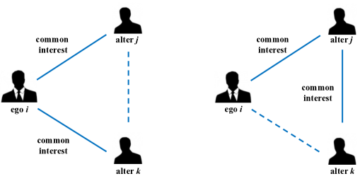
Figure 1: Two different schemes of relationships based on mutual common interests, from an ego and its ego network (left) and from an ego and a path of length 2 (right).

The behavior of nodes is often highly influenced by the behavior of their neighbors or community members [22, 49]. From this point of view, the clustering coefficient is one of the main measures used to understand the level of cohesion around a node.

The generalized concept of clustering coefficient presented here describes community structures which are not established, but are indirectly induced by strong cooperations among the formally linked nodes. More specifically, the existence of a powerful link between two nodes is assumed to be able to form the connection between nodes that are disconnected but adjacent to the considered ones.

In this respect, social motivations from the perspective of a single node (ego) support the study of the proposed generalized clustering coefficient. In particular, the knowledge for two alters of a common ego increases the opportunities for them to meet since they could be engaged in similar interests, which would ultimately provide a basis for them to trust one another [19]. Moreover, social psychology suggests that an ego has an incentive to connect to its alters in order to reduce its isolation [26]. An ego might also be interested in connecting to its neighbors for proximity reasons, taking into consideration the shortest path distance between them [9].

Here, we also consider the possibility of having an indirect connection of an ego with an alter of one of its alters. Therefore, we consider two forms of engagements between an ego and various alters, as shown in Figure 1. More details on the figure will be given in Section 5.3.

The perspective adopted here represents the basis for several real-world cases. For example, in [28], affiliation networks allow one to observe the connections among individuals indirectly, i.e. not through directly observed social interactions, while in [9], a new measure of the clustering coefficient is proposed, with applications in the study of segregation and homophily. Finally, in biology, gene expression data can be studied with the weighted clustering coefficient in order to reveal differences between normal and tumour networks [29].

It is also worth mentioning how the concepts of triples introduced here could relate to the issue of link formation. Indeed, the presence of a strong connection between two units would probably induce cooperation also among the units connected with those considered in the near future. In this regard, link creation was studied from the perspective of the clustering coefficient. We mention [30], where authors investigate the origins of homophily and tie formation by means of triadic closures and proximity, and [42], where a new method for triple estimation is presented.

3 Preliminaries and notations about graph theory

For the convenience of the reader, we shall now provide some preliminaries and notations. The classical mathematical abstraction of a network is a graph $G=(V,E)$, where $V$ is the set of $N$ nodes (or vertices) and $E$ is the set of $M$ links (or edges) stating the relationships among the nodes. We refer to a node by an index $i$, meaning that we allow a one-to-one correspondence between an index in $\{1,\dots,N\}$ and a node in $V$. The set $E$ can be conceptualized through the adjacency matrix $\mathbf{A}=(a_{ij})_{i,j=1,\dots,N}$, whose generic element $a_{ij}$ is 1 if the link between $i$ and $j$ exists and 0 otherwise. The graph is undirected when $a_{ij}=a_{ji}$, for each $i,j=1,\dots,N$, and directed otherwise. The degree $d_{i}$ of the node $i$ is a nonnegative integer representing the number of links incident upon $i$.

In this paper, we examine weighted networks, and we refer to a weighted adjacency matrix $\mathbf{W}$ whose elements $w_{ij}\geq 0$ represent the weights on the link connecting nodes $i$ and $j$, with $i,j=1,\dots,N$. Clearly, $w_{ij}=0$ stands for absence of a link between $i$ and $j$. Thus, $w_{ij}$ denotes the intensity of the interactions between two nodes $i$ and $j$ and allows for the modeling of the ties’ strength of the observed system.

4 Literature review on the clustering coefficient for unweighted and weighted networks

4.1 Unweighted networks

The local clustering coefficient can be defined for any vertex $i=1,\dots,N$ and captures the capacity of edge creations among neighbors, i.e. the tendency in the network to create stable groups [53]. Thus, the cohesion around a vertex $i$ is quantified by the local clustering coefficient $C_{i}$ defined as the number of triangles $t_{i}$ in which vertex $i$ participates normalized by the maximum possible number of such triangles:

$$C_{i}=\frac{2t_{i}}{d_{i}(d_{i}-1)}.$$ (1)

The local clustering coefficient quantifies how a node takes part in a cohesive group. Therefore, $C_{i}=0$ if none of the neighbors of a node are connected and $C_{i}=1$ if all of the neighbors are linked.

The value of the local clustering coefficient is influenced by the nodes degrees. A node with several neighbors is likely to be embedded in fewer closed triangles; hence, it has a smaller local clustering coefficient when compared to a node linked to fewer neighbors, where they are more likely to be clustered in triangles [4].

The clustering coefficient for a given graph is computed in two classical modes [37]. The first is the averaged clustering coefficient $\overline{C}$, given as the average of all the local clustering coefficients, while the second, called the global clustering coefficient and denoted by $C_{G}$, is defined as the ratio among three times the number of closed triangles in the graph and the number of its triples, i.e. the number of 2-paths among three nodes.

Note that both $\overline{C}$ and $C_{G}$ assume values from $0$ to $1$ and are equal to $1$ in case of a clique, i.e. a fully coupled network. In real networks, the evidence shows that nodes are inclined to cluster into densely connected groups [21, 51] and the difficulty of comparing the values of clustering nodes with different degrees makes the average value of local clustering sensitive to the way in which degrees are distributed across the whole network.

The quantities $\overline{C}$ and $C_{G}$ are specifically tailored to unweighted networks, and they cannot be satisfactorily employed to describe the community structure of the network in the presence of weights on links and when arcs are of the direct type.

The next section is devoted to the analysis of the more general weighted cases.

4.2 Weighted networks

In many real networks, connections are relevant not only in terms of the classical binary state – whether they exist or do not exist – but also with regards to their strength which, for any node $i=1,\dots,N$, is defined as:

$$s_{i}=\sum_{j=1}^{N}w_{ij}.$$ (2)

The introduction of weights and strengths extends the study of the macroscopic properties of the network by adding some forms of entity of connections and capability to the mere interactions. In particular, the strength integrates information about the vertex connectivity and the weights of its links [6]. It is considered a natural measure of the importance or centrality of a vertex $i$. Indeed, the identification of the most central nodes represents a major issue in network characterization [23].

In [6], Barrat et al. combine the topological information of the network with the distribution of weights along links, and define the weighted clustering coefficient for a node $i=1,\dots,N$ as follows:

$$\tilde{C}_{i,B}=\frac{1}{s_{i}(d_{i}-1)}\sum_{j,k\in V}\frac{w_{ij}+w_{ik}}{2}a_{ij}a_{jk}a_{ik}.$$ (3)

This coefficient is a quantity of the local cohesiveness, which considers the importance of the clustered structure by taking into account the intensity of the interactions found on the local triangles. This measure counts, for each triangle created in the neighborhood of the node $i$, the weight of the two related edges. The authors refer not to the mere number of the triangles in the neighborhood of a node but also to their total relative weight with respect to the strength of the nodes.

The normalization factor $s_{i}(d_{i}-1)$ accounts for the strength $s_{i}$ and the maximum possible number of triangles in which the node $i$ may participate, and it ensures that $0\leq\tilde{C}_{i,B}\leq 1$. The definition of $\tilde{C}_{i,B}$ recovers the topological clustering coefficient in the case where $w_{ij}$ is constant, for each $j$.

Therefore, the authors introduce the weighted clustering coefficient averaged over all nodes of the network, say $C^{W}$, and over all nodes with degree $d$, say $C^{W}(d)$. These measures offer global information on the correlation between weights and topology by comparing them with their topological analogs.

Note that $s_{i}=d_{i}(s_{i}/d_{i})=d_{i}\langle w_{i}\rangle$, so $\tilde{C}_{i,B}$ can be written as:

$$\tilde{C}_{i,B}=\frac{1}{d_{i}(d_{i}-1)}\sum_{j,k\in V}\frac{w_{ij}+w_{kj}}{2\langle w_{i}\rangle}a_{ij}a_{jk}a_{ik}$$ (4)

where $\langle w_{i}\rangle=\sum_{j}w_{ij}/{d_{i}}$. In such equation the contribution of each triangle is weighted by a ratio of the average weight of the two adjacent links of the triangle to the average weight $\langle w_{i}\rangle$.

Thus, $\tilde{C}_{i,B}$ compares the weights related with triangles to the average weight of edges connected to the local node.

Zhang and Horvath [56] describe the weighted clustering coefficient in the context of gene co-expression networks. Unlike the unweighted clustering coefficient, the weighted clustering coefficient is not inversely related to the connectivity. Authors show a model that reveals how an inverse relationship between the clustering coefficient and connectivity occurs from hard thresholding. In formula:

$$\tilde{C}_{i,Z}=\frac{\sum_{j,k\in V}\hat{w}_{ij}\hat{w}_{jk}\hat{w}_{ik}}{(\sum_{k\in V}\hat{w}_{ik})^{2}-\sum_{k}\hat{w}_{ik}^{2}}$$ (5)

where the weights have been normalized by $\max(w)$. The number of triangles around the node $i$ can be written in terms of the adjacency matrix elements as $t_{i}=1/2\sum_{i,k\in V}a_{ij}a_{jk}a_{ik}$ and the numerator of the above equation is a weighted generalization of the formula. The denominator has been selected by considering the upper bound of the numerator, ensuring $\tilde{C}_{i,Z}\in[0,1]$ . The equation (5) can be written as:

$$\tilde{C}_{i,Z}=\frac{\sum_{j,k\in V}\hat{w}_{ij}\hat{w}_{jk}\hat{w}_{ik}}{\sum_{j,k\in V:j\neq k}\hat{w}_{ij}\hat{w}_{ik}}$$ (6)

In Grindrod [25], a similar definition has been shown; indeed, the edge weights are considered as probabilities such that in an ensemble of networks, $i$ and $j$ are linked with probability $\hat{w}_{ij}$. Finally, Holme et al. [28] discuss the definition of weights and express a redefined weighted clustering coefficient as:

$$\tilde{C}_{i,H}=\frac{\sum_{j,k\in V}w_{ij}w_{jk}w_{ik}}{\max(w)\sum_{j,k\in V}w_{ij}w_{ik}}=\frac{\mathbf{W}^{3}}{(\mathbf{W}\mathbf{W}_{max}\mathbf{W})_{ii}}$$ (7)

where $\mathbf{W}_{max}$ indicates a matrix where each entry equals $\max(w)$. This equation seems similar to those in [56], though, $j\neq k$ is not required in the denominator sum.

Onnela et al. [38, 39] refer to the notion of motif, defining it as a set (ensemble) of topologically equivalent subgraphs of a network. In cases of weighted systems, it is necessary to deal with intensities rather than numbers of occurrence. Moreover, the latter concept is considered as a special case of the former one. For the authors, the triangles are among the simplest nontrivial motifs and have a crucial role as one of the classic quantities of network characterization in defining the clustering coefficient of a node $i$. They propose a weighted clustering coefficient taking into consideration the subgraph intensity, which is defined as the geometric average of subgraph edge weights. In formula:

$$\tilde{C}_{i,O}=\frac{2}{d_{i}(d_{i}-1)}\sum_{j,k\in V}(\hat{w}_{ij}\hat{w}_{ik}\hat{w}_{jk})^{1/3}$$ (8)

where $\hat{w}_{ij}=w_{ij}/\max_{j\in V}(w_{ij})$ are the edge weights normalized by the maximum weight in the network of the edges linking $i$ to the other nodes of $V$.

Formula (8) shows that triangles contribute to the creation of $\tilde{C}_{i,O}$ according to the weights associated to their three edges. More specifically, $\tilde{C}_{i,O}$ disregards the strength of the local node and measures triangle weights only in relation to the maximum edge weight.

Moreover, $\tilde{C}_{i,O}$ collapses to $C_{i}$ when, for each $i,j\in V$, one has $w_{ij}=a_{ij}$, and is thus in the unweighted case.

5 The generalized clustering coefficient

This section contains our proposal for a new definition of the clustering coefficient of weighted networks. Based on a novel concept of triangles, this definition includes the presence of real indirect connections among individuals. For our purpose, we first provide and discuss the definition of the triangles, and then we introduce the clustering coefficient.

5.1 Generalized triples

Here, we propose a generalization of the concept of triangle, and rewrite accordingly the coefficient $C_{i}$ in (1) for the case of weighted networks.

Definition 5.1

Let us consider a weighted non-oriented graph $G=(V,E)$ with vertices $V=\{1,\dots,N\}$, symmetric adjacent matrix $\mathbf{A}=(a_{ij})_{i,j=1,\dots,N}$ and weight matrix $\mathbf{W}=(w_{ij})_{i,j=1,\dots,N}$, with nonnegative weights. Moreover, let us take $\alpha,\beta\in[0,\infty)$ and a function $F:[0,+\infty)^{2}\to[0,+\infty)$ which is not decreasing in its arguments.

For each triple of distinct vertices $i,j,k\in V$, a subgraph $t=(\{i,j,k\},E_{T})$ is a generalized triangle (or, simply, a triangle) around $i$ if one of the following conditions are satisfied:

• $a_{ij}=a_{ik}=a_{jk}=1$;

• $a_{ij}=a_{ik}=1$, $a_{jk}=0$ and $F(w_{ij},w_{ik})\geq\alpha$;

• $a_{ij}=a_{jk}=1$, $a_{ik}=0$ and $F(w_{ij},w_{jk})\geq\beta$.

Herein we denote the elements of types $T_{2}$ and $T_{3}$ as triples since they are not really triangles since they are not contained in $G$. They can be seen as a generalization of triangles by including the missing side, which is induced by conditions on the weights of the two existing edges.

We denote the set of generalized triangles associated to case $T_{h}$ as $\mathcal{T}^{(i)}_{h}$, for $h=1,2,3$. By definition, $\mathcal{T}_{1}^{(i)}\cap\mathcal{T}_{2}^{(i)}=\mathcal{T}_{1}^{(i)}\cap\mathcal{T}_{3}^{(i)}=\mathcal{T}_{2}^{(i)}\cap\mathcal{T}_{3}^{(i)}=\emptyset$. We denote the set collecting all the triangles by $\mathcal{T}^{(i)}=\mathcal{T}_{1}^{(i)}\cup\mathcal{T}_{2}^{(i)}\cup\mathcal{T}_{3}^{(i)}$.

Figure 2 reports the three different type of triangles, respectively $T_{1}$, $T_{2}$ and $T_{3}$. Clearly, in the case of $T_{1}$, the concept of triangle given in Definition 5.1 coincides with the standard one.

Note that with $N$ nodes, the maximum number of possible triangles is $|\mathcal{T}_{1}|^{*}=\max|\mathcal{T}_{1}|=\binom{N}{3}$. This is the case of a clique with $C_{i}=1$, for each $i\in V$.

When considering the maximum number of candidates triangles for a node $i$ to belong to $T_{2}$, it is $|\mathcal{T}_{2}^{(i)}|^{*}=\max|\mathcal{T}_{2}^{(i)}|=\binom{d_{i}}{2}$. Then, in this case for the node $i$ the number of triples is $|\mathcal{T}_{2}^{(i)}|=|\mathcal{T}_{2}^{(i)}|^{*}-|\mathcal{T}_{1}^{(i)}|$.

Triples in $T_{3}$ for node $i$ are the paths of length $2$, which can be computed by considering the square of the adjacency matrix. Indeed, the number of different paths of length $2$ from $i$ to $k$ equals the entry $a_{ik}$ of $A^{2}$ [43]. For a given row $i$ of $A^{2}$, the sum of the element (excluding the element $a_{ii}$) equals the maximum potential number of triples of type $T_{3}$.

Figure 2 shows the types of triangles, without emphasis on the conditions on the weights.

Figure 2: Types of triangles: $T_{1}$ (left), $T_{2}$ (center), $T_{3}$ (right).

5.2 Conceptualization of the generalized clustering coefficient

Under Definition 5.1, we can introduce a generalization of the clustering coefficients presented in Formula (1) for weighted networks.

Definition 5.2

Given a graph $G=(V,E)$ and a node $i\in V$, the generalized unweighted clustering coefficient of $i$ is

$$C_{i}^{(g)}=\frac{|\mathcal{T}^{(i)}|}{D_{i}}$$ (9)

where $D_{i}=\frac{d_{i}(d_{i}-1)}{2}+|\{j\in V:\Delta_{min}(i,j)=2\}|$, where $\Delta_{min}(i,j)$ is the minimum distance between the nodes $i$ and $j$.

The term unweighted in Definition 5.2 points to the absence of $w$’s in the coefficient in (9). However, weights intervene in the identification of the triangles, according to Definition 5.1. In particular, formula (9) extends (1). As an example, notice that $C_{i}^{(g)}=C_{i}$ in the clique case.

5.3 Implications of the generalized clustering coefficient and equivalent graphs

The classical local clustering coefficient $C_{i}$ not only captures the proportion of closed triples on all possible triples depending on the degree of the ego/node $i$, but it also identifies its level of cohesion. While the averaged clustering coefficient $\overline{C}$ captures the whole level of network cohesion.

The proposed generalized clustering coefficient extends the same setting also to the triples in $T_{2}$ and $T_{3}$, i.e. it is the proportion of triangles of type $T_{1}$, $T_{2}$ and $T_{3}$ on all possible triangles. This process depends not only on the degree of the ego but also on the two thresholds $\alpha$ and $\beta$, which take into account the strength profile around the ego, and thus have the possibility of creating triangles $T_{2}$ and $T_{3}$.

The values of the generalized clustering coefficient are $0\leq C_{i}^{(g)}\leq 1$ as well as for the averaged measure $C^{(g)}$ and differ from the usual measure because they depend on the thresholds $\alpha$ and $\beta$.

Importantly, $C_{i}^{(g)}$ assumes unitary value not only in the clique case, but also when any missing link is compensated by the high weights of the other two links, i.e. when simultaneously $\alpha<F(w_{ij},w_{ik}),\forall i,j,k$ and $\beta<F(w_{ij},w_{jk}),\forall i,j,k$. This property of the generalized clustering coefficient is very relevant, since it allows one to extend the sense of community given by the classical clustering coefficient to the case of indirect links being present, as seen in the definition of triples $T_{2}$ and $T_{3}$.

The triples $T_{2}$ and $T_{3}$ can be described as follows (see Figure 1). The former describes a situation in which an ego $i$ has a direct relationship with alters $j$ and $k$. One can say that there exists a triangle among the three if the strength of the connections of $i$ with the others is sufficiently high – in the sense described by function $F$. The idea is that the cooperation and/or the common interests between $i$ and the alters is so effective and fruitful that the presence of a direct link between $j$ and $k$ is not required.

The latter case is associated to the presence of a strong link between $i$ and $j$ and between $j$ and $k$, always in terms of the entities of the weights – in the sense described by function $F$. In this peculiar situation, the node $j$ represents the intermediate alter letting also the (indirect) collaboration between $i$ and $k$ be possible.

Finally, the thresholds have a double meaning. In fact, if we consider a network in which interactions between alters could be facilitated, an external decision-maker could implement policies aiming to define the correspondent values of $\alpha$ and $\beta$ low. For example, in the case of inter-organizational innovation networks, the presence of triangles is positively related to the establishment of stable groups, as well as to the amount of produced efforts, the straightening of transitive relationships and the innovation capacity [13, 21].

On the other hand, if a decision-maker were to prevent interactions among alters, the policies with correspondent values $\alpha$ and $\beta$ could be deemed sufficiently large. Such an instance can be found in the prevention of community formation in criminal organizations [20, 36].

5.3.1 Equivalent graphs

Triangles $T_{1}$, $T_{2}$ and $T_{3}$ also serve in deriving topological information from the graph. In particular, assume that $\alpha=\beta=0$, so that the number of $T_{2}$ and $T_{3}$ around each node does not depend on the specific selection of function $F$. In this case, we know that $|\mathcal{T}_{2}^{(i)}|=\binom{d_{i}}{2}$, meaning we are able to infer the degree of the node $i$ by the knowledge of the number of triangles of type $T_{2}$ around it. Conversely, $|\mathcal{T}_{3}^{(i)}|$ represents the number of existing paths of length 2 having $i$ as one of the extreme nodes. By collecting the number of the triangles $T_{1}$, $T_{2}$ and $T_{3}$ for each node of the graph, we are able to identify a class of graphs.

Formally, consider a $3\times N$ matrix collecting $|\mathcal{T}_{1}^{(i)}|$, $|\mathcal{T}_{2}^{(i)}|$ and $|\mathcal{T}_{3}^{(i)}|$, for each node $i\in V$. Denote by $\mathcal{M}^{3,N}(\mathbb{N})$ the set of all the matrices with dimension $3\times N$ and filled by integer nonnegative numbers.

Thus, each matrix $\mathbf{M}\in\mathcal{M}^{3,N}(\mathbb{N})$ identifies a non-unique graph that has $N$ nodes and edges described by $\mathbf{M}$. We refer to such a matrix as the triangles matrix. In this sense, $\mathbf{M}$ can be viewed as an equivalent class in the set of the graph with $N$ nodes, where two graphs $G_{1}$ and $G_{2}$ are said to be equivalent when they share the same matrix $\mathbf{M}$.

Figure 3 and the matrix in (1) provide an example of two equivalent classes, along with their common triangles matrix $\mathbf{M}$. In particular, notice that matrix $\mathbf{M}$ is the same for the two considered graphs, thus suggesting that the equivalent class identified by $\mathbf{M}$ contains more than one graph.

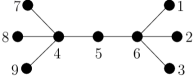
Figure 3: Two equivalent graphs, according to the equivalence defined through the triangles matrix. In this case, the triangles matrix $\mathbf{M}$ associated to the graphs is given in Table 1.

node $i$	$|\mathcal{T}_{1}^{(i)}|$	$|\mathcal{T}_{2}^{(i)}|$	$|\mathcal{T}_{3}^{(i)}|$
1	0	0	3
2	0	0	3
3	0	0	3
4	0	5	1
5	0	1	6
6	0	5	1
7	0	0	3
8	0	0	3
9	0	0	3

Table 1: Triangles matrix $\mathbf{M}$ associated with the graphs in Figure 3.

6 Applications

Herein we considered the analysis of the generalized clustering coefficient on two empirical networks: the network among the $500$ busiest US commercial airports [15] and the nervous system of the nematode Caenorhabditis elegans [53, 54]. The data processing, the network analysis and all simulations were conducted using the software R [44] with the igraph package [17]. The datasets were obtained from the $R$ packege tnet, authored by Tore Opsahl [47]. Code in the $R$ programming language is available upon request.

For the sake of readability we report in Table 2 the notations used hereafter.

Symbol	Meaning
$t_{i}$	Triangles around node $i$.
$T_{h}$	Triples of type $h=1,2,3$.
$\mathcal{T}^{(i)}_{h}$	Set of triples of node $i$ associated to case $T_{h}$, for $h=1,2,3$.
$|\mathcal{T}^{(i)}_{h}|$	Cardinality of the set $\mathcal{T}^{(i)}_{h}$
$F_{i}$	Function of type $i=1,2,3,4.$
$\alpha$	Threshold for triples $T_{2}$
$\beta$	Threshold for triples $T_{3}$
$C_{i}$	Local clustering coefficient
$\overline{C}$	Averaged clustering coefficient
$C_{G}$	Global clustering coefficient
$C_{i}^{(g)}$	Generalized clustering coefficient

Table 2: Table of notation.

6.1 General settings

In the empirical experiments, we consider four cases of function $F$:

• sum of the weights is greater than the correspondent coefficient: $w_{ij}+w_{ik}\geq\alpha$ and $w_{ij}+w_{jk}\geq\beta$;

• average of the weights is greater than the correspondent coefficient: $(w_{ij}+w_{ik})/2\geq\alpha$ and $(w_{ij}+w_{jk})/2\geq\beta$;

• minimum of the weights is greater than the correspondent coefficient: $\min\{w_{ij},w_{ik}\}\geq\alpha$ and $\min\{w_{ij},w_{jk}\}\geq\beta$;

• maximum of the weights is greater than the correspondent coefficient: $\max\{w_{ij},w_{ik}\}\geq\alpha$ and $\max\{w_{ij},w_{jk}\}\geq\beta$.

The selection of the specific function $F$ – to be implemented among $F_{1},\ldots,F_{4}$ defined above – provides further insights into the interpretation of the triples of type $T_{2}$ and $T_{3}$. Indeed, once $\alpha$ and $\beta$ are kept fixed, then $F_{1}$ and $F_{2}$ state that both weights of the considered edges should be taken into account in an identical way by considering their mere aggregation in the former case or their mean in the latter one. When considering functions $F_{3}$ and $F_{4}$, only one of the weights is relevant for the measurement of the strength of the connections – the minimum weight and the maximum one, respectively. Naturally, the former case is more restrictive than the latter one, since it implicitly assumes that both weights should be greater than $\alpha$ or $\beta$ for having a triples of type $T_{2}$ or $T_{3}$.

Social sciences suggest other functions $F$’s to be considered in Definition (5.1) to capture certain peculiarities of the system under observation. Notice also that $|\mathcal{T}_{2}^{(i)}|$ and $|\mathcal{T}_{3}^{(i)}|$ are not increasing functions of $\alpha$ and $\beta$, respectively, as Definition (5.1) implies.

For the simulations, the value of $\alpha$ and $\beta$ are $\alpha,\beta=\{0,250000,500000,750000,1000000,$ $1250000,1500000,1750000,2000000,2225000\}$ for the US airports network and $\alpha,\beta=\{0,5,10,15,20,25,30,35,40,45,50,55,60,65,70\}$ for the C.elegans network. The max values were chosen on the ground that function $F_{1}$ could possibly be true also when considering arcs with the higher weights. As such, $10$ runs were implemented for each considered value. Thus, we performed $100$ computations for the US airports network and $150$ computations for the C.elegans network.

According to Definition (5.1), $\mathcal{T}_{2}^{(i)}$ and $\mathcal{T}_{3}^{(i)}$, i.e. the triangles for every node in a network, can be computed considering $\alpha=0$ and $\beta=0$. Concerning the sets $\mathcal{T}_{1}^{(i)}$, such triangles can be easily computed by a built-in function in $igraph$.

6.2 Analysis of the US commercial airports network

The US commercial airports network has $n=500$ nodes denoting airports and $m=2980$ edges representing flight connections. In this network, weights are the number of seats available on that connections in 2010. The network has both small-world and scale-free organization with $\gamma\simeq 1.8$ [7].

In Figure 4 (left) we show the network visualization, while Table 3 reports some basic measures: the density $\delta$, the averaged clustering coefficient $\overline{C}$, the global clustering coefficient $C_{G}$ and the minimum, maximum and average degree, weight and strength.

In Figure 5 (left) we report the strength distribution for this network, with the strength $s_{i}$ as the sum of the weights of the links incident on $i$, while Figure 6 (left) uses a histogram to display the weights.

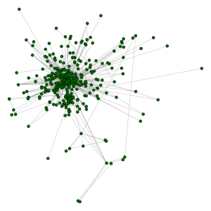
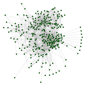
Figure 4: Network visualization for the US airports (left) and C.elegans (right).

Network	$\delta$	$\overline{C}$	$C_{G}$	$k_{min}$	$k_{max}$	$\overline{d}$
US airports	0.0239	0.617	0.351	1	145	11.92
C.elegans	0.0314	0.228	0.121	1	134	9.26
Network	$w_{min}$	$w_{max}$	$\overline{w}$	$s_{min}$	$s_{max}$	$\overline{s}$
US airports	9	2253992	152320.19	9416	49316361	1815656.66
C.elegans	1	61	4.198	1	1700	38.86

Table 3: Basic measures for the networks under analysis.

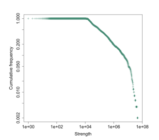
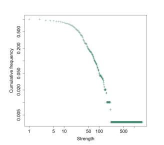
Figure 5: Strength distributions for the US airports (left) and C.elegans (right) networks.

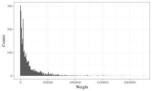
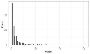
Figure 6: Histogram displaying weights for US airports (left) and C.elegans (right) networks.

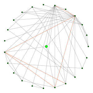
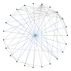
Figure 7: $2-$step ego network of node $n=488$ of the US airports network and triples $\mathcal{T}_{2}^{(488)}$ (left) and $\mathcal{T}_{3}^{(488)}$ (right).

Functioning as an example, Figure 7 shows the arcs composing the triples in $\mathcal{T}_{2}^{(488)}$ and in $\mathcal{T}_{3}^{(488)}$ for the neighborhood of order $2$ of node $n=488$, i.e. its 2-step ego network. Such a node has a degree $d_{488}=5$, a second order neighborhood of cardinality $18$ and a local clustering coefficient $C_{488}=0.5$, because $5$ triangles are closed out of a theoretical $10$.

Thus, $|\mathcal{T}_{2}^{(488)}|=5$ while triangles in $\mathcal{T}_{3}^{(488)}$ are computed obtaining $|\mathcal{T}_{3}^{(488)}|=22$. Note that the blue arcs in the right panel of Figure 7 are $18(<22)$ because some arcs can be mentioned twice in the set, since arc $(i,k)$ can derive from $i\rightarrow j\rightarrow k$ as well as from $i\rightarrow l\rightarrow k$.

The generalized clustering coefficient has value $C_{488}^{(g)}=0.0632$, which is much lower than $C_{488}$ since the proportion of closed triangles when $\alpha=0$ and $\beta=0$ is smaller than the basic setting.

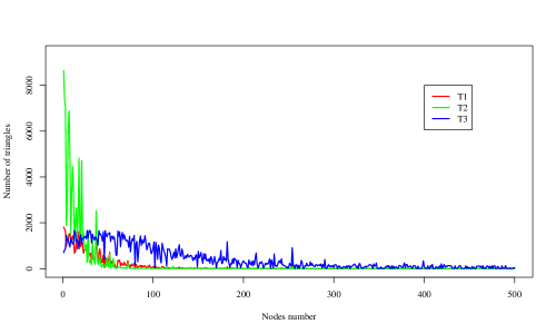
Figure 8: US airports. Comparison between the number of triangles $T_{1}$, the number of potential triples $T_{2}$ and the number of potential triples $T_{3}$.

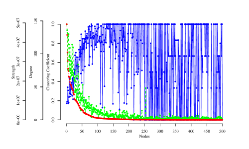
Figure 9: US airports. Comparison between local clustering coefficient (blue points), degree (red points) and strength (green points).

Figure 8 for the US airports network reports three curves for each node: the total number of triangles $|\mathcal{T}_{1}^{(i)}|$, the number of potential triples of type $|\mathcal{T}_{2}^{(i)}|$ and the number of potential triples of type $|\mathcal{T}_{3}^{(i)}|$. Figure 9 compares the degree $d_{i}$ and the local clustering coefficient $C_{i}$ for each node $i$. Note that nodes in the US airports network are enumerated in non-increasing order of their degree and the nodes with indices until $i\simeq 100$ have values of degree and clustering coefficient, which allow for a large number of triples $T_{2}$ and a significant number of triples $T_{3}$. Then, when the degree decreases and the local clustering coefficient increases, the local neighborhoods preclude the formation of triangles.

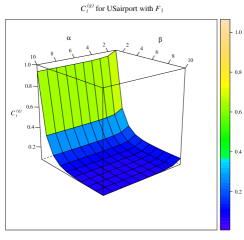
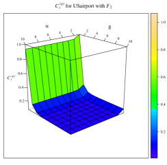
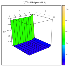
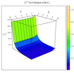
Figure 10: US airports: Average values of $C_{i}^{(g)}$ for cases $F_{1}$ (upper left), $F_{2}$ (upper right), $F_{3}$ (lower left) and $F_{4}$ (lower right).

Figure 10 shows the averaged values of the generalized clustering coefficient $C_{i}^{(g)}$ for the US airports network when considering the four different functions $F_{1},F_{2},F_{3}$ and $F_{4}$. In each figure, the values are presented for every combination of $\alpha$ and $\beta$ while the horizontal axis reports the values of $C_{i}^{(g)}$ as averaged over every node in the network. As expected, higher values of $C_{i}^{(g)}$ are obtained for lower values of $\alpha$ and $\beta$ and, globally, we have a non-increasing trend with a higher slope for functions $F_{2}$ and $F_{3}$ since the average and the min functions smooth the values, thus indicating that the functions are true only for small values of weights. Regarding $F_{1}$ and $F_{4}$, they are more prone to being true for higher values of arc weight, meaning the slope declines at slower rate.

A common behavior for all four cases is that the magnitude of $C_{i}^{(g)}$ is more dependent on triples $T_{2}$ than those in $T_{3}$. This is due to the tendency of high-degree nodes to have a higher strength. Therefore, the functions are more prone to being true for triples $T_{2}$ than for triples in $T_{3}$ since the adjacent links could possibly lie in a low-degree node with a low value of strength.

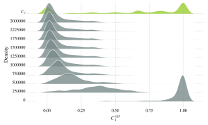
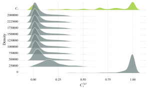
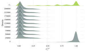
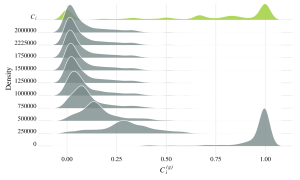
Figure 11: US airports. Density of $C_{i}^{(g)}$ for different values of $\alpha$ when $\beta=0$ for cases $F_{1}$ (upper left), $F_{2}$ (upper right), $F_{3}$ (lower left) and $F_{4}$ (lower right).

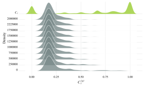
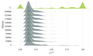
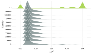
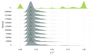
Figure 12: US airports. Density of $C_{i}^{(g)}$ for different values of $\beta$ when $\alpha=0$ for cases $F_{1}$ (upper left), $F_{2}$ (upper right), $F_{3}$ (lower left) and $F_{4}$ (lower right).

In order to study the evolution of the generalized clustering coefficient $C_{i}^{(g)}$ when varying $\alpha$ and $\beta$, we provide a series of diagrams in which, for the network under examination, the density of the $C_{i}^{(g)}$ values are reported when considering fixed values of $\alpha=0$ or $\beta=0$ and when the other thresholds varing.

In particular, for the network under observation, Figure 11 shows different density values for each $\alpha$ when $\beta=0$, and Figure 12 shows each $\beta$ when $\alpha=0$. All the figures also report the density values of the local clustering coefficient $C_{i}$ (colored in light green).

When $\beta=0$ (see Figure 11) we can observe the contribution of triples in $T_{2}$ to $C_{i}^{(g)}$. The density of $C_{i}^{(g)}$ is more concentrated around the max value $1$ when $\alpha=0$; however, when $\alpha$ starts to grow the values shift closer to $0$.

For $\alpha=0$, Figure 12 highlights that $C_{i}^{(g)}$ receives a small contribution from triples in $T_{3}$ and the values lay around $0$ as soon $\beta$ grows.

The density of $C_{i}$ shows that values are concentrated mainly around $0$ and $1$, meaning that many airports have a single connection with another airport or have a strong cohesive structure. When studying $C_{i}^{(g)}$ it is possible to infer that some airports with a single connection with a common node have weight profiles that involve a certain level of interaction for a given threshold. For example, for low values of $\alpha$ passengers from or to airports $j$ and $k$ often use connection $i$, thus suggesting the establishment of a direct and intended connection between the two airports. This is not true when considering triples in $T_{3}$; here the analysis suggests that a direct connection among $i$ and $k$ is less useful and passengers still prefer to fly by $j$.

6.3 Analysis of the C.elegans network

The network of nematode Caenorhabditis elegans (C.elegans) has $n=296$ nodes representing neurons and $m=1370$ edges occurring when two neurons are connected by either a synapse or a gap junction; for each edge, weights are equal to the number of junctions between nodes $i$ and $j$. The network has a scale-free organization with $\gamma\simeq 3.14$ [5, 48].

In Figure 4 (right) we show the network visualization, while Table 3 reports the basic measures. Note that for this network we considered the giant component of $296$ nodes while the complete network is composed of $306$ nodes.

In Figure 5 (right) we report the strength distributions for the C.elegans network. Note that the two networks under observation are very different, especially in the distribution of low and high values of strength. The weight profiles in Figure 6 confirm such differences, which are mostly caused by a difference of scale in the values.

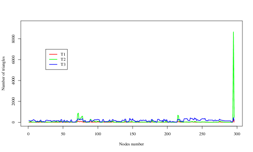
Figure 13: C.elegans. Comparison between the number of triangles $T_{1}$, the number of potential triangles $T_{2}$ and the number of potential triangles $T_{3}$.

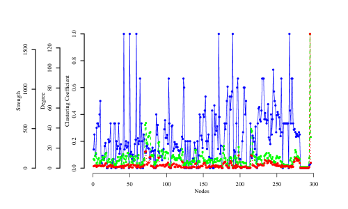
Figure 14: C.elegans. Comparison between local clustering coefficient (blue points), degree (red points) and strength (green points).

The analysis of Figures 13 and 14 depicts a very different picture for the C.elegans network when compared to the US airports network. Again, Figure 13 reports the three curves representing the total number of triangles $|\mathcal{T}_{1}^{(i)}|$, the number of potential triples of type $|\mathcal{T}_{2}^{(i)}|$ and the number of potential triples of type $|\mathcal{T}_{3}^{(i)}|$. Figure 14 compares the degree $d_{i}$ and the local clustering coefficient $C_{i}$ for each node $i$. Note that in these benchmark instances, nodes are enumerated without a particular rule.

In the C.elegans networks, nodes with a higher degree have relatively small values of local clustering coefficient, whilst nodes with a smaller degree have, in general, higher values of local clustering coefficient. This means that small-degree nodes tends to form dense local neighborhoods, while the neighborhood of hubs is much sparser. Such observations motivate the limited number of triples in $T_{2}$ because, for each node $i$, they are in number of $\binom{d_{i}}{2}-|\mathcal{T}_{1}^{(i)}|$, thus implying that denser neighborhoods have a smaller number of possible triples.

Note in Figure 13 that node $i=295$ has a peak because $|\mathcal{T}_{2}^{(i)}|=8658$ when the thresholds $\alpha$ and $\beta$ are null (this is the case of all potential triples). This is motivated by the fact that its particular neighborhood is composed of a limited number of triangles in which it is embedded ($|\mathcal{T}_{1}^{(295)}|=253$ and $C_{295}=0.028$) despite its degree ($d_{295}=134)$. Choosing two edges on $134$ leads to $8911$ potential triples of type $T_{2}$ and subtracting $253$ results in $8658$. Such a remarkable presence of triples of type $T_{2}$ for a single node for the case of $\alpha=\beta=0$ suggests that the C.elegans network is star-shaped.

Similar arguments can be considered for $T_{3}$; indeed, we have a small number of potential triples for both small-degree nodes and hubs, since low values of degree allow for a smaller amount of transitive closure.

Figure 15 reports the same plots for the C.elegans network and same comments on the general behavior can be repeated as for the previous network. The main difference is the gentler slope, which occurs due to the profile of weight distribution being less concentrated on lower values when compared to the US airports network (see also Figure 6).

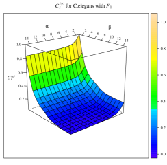
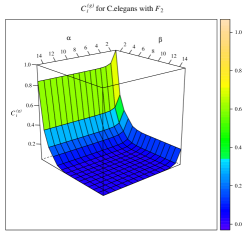
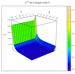
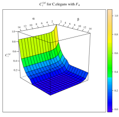
Figure 15: C.elegans. Average values of $C_{i}^{(g)}$ for cases $F_{1}$ (upper left), $F_{2}$ (upper right), $F_{3}$ (lower left) and $F_{4}$ (lower right).

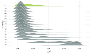
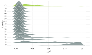
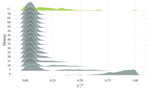
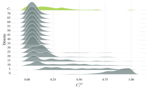
Figure 16: C.elegans. Density of $C_{i}^{(g)}$ for different values of $\alpha$ when $\beta=0$ for cases $F_{1}$ (upper left), $F_{2}$ (upper right), $F_{3}$ (lower left) and $F_{4}$ (lower right).

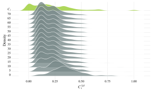
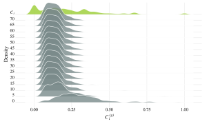
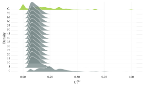
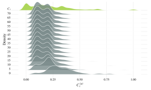
Figure 17: C.elegans. Density of $C_{i}^{(g)}$ for different values of $\beta$ when $\alpha=0$ for cases $F_{1}$ (upper left), $F_{2}$ (upper right), $F_{3}$ (lower left) and $F_{4}$ (lower right).

The analysis of the C.elegans network is completed with the series of diagrams in which the density of the $C_{i}^{(g)}$ values are reported when considering fixed values of $\alpha=0$ or $\beta=0$ and varying the other threshold.

Even for this network, Figure 16 shows different density values for each $\alpha$ when $\beta=0$ and Figure 17 for each $\beta$ when $\alpha=0$. Note that all the figures report the density values of the local clustering coefficient $C_{i}$ (colored in light green).

When $\beta=0$ (see Figure 16) the contribution of triples in $T_{2}$ makes the density of $C_{i}^{(g)}$ more concentrated around the max value $1$ when $\alpha=0$; when $\alpha$ starts to grow the values shift closer to $0$. Such an effect is present in both the networks under observation but it is more evident for the C.elegans.

Similarly, at the US airports network, for $\alpha=0$, Figure 17 highlights that $C_{i}^{(g)}$ receives a small contribution from triples in $T_{3}$ and the values lay around $0$ as soon as $\beta$ grows.

The observation of the way in which $C_{i}$ density lays seems to affirm that the network has a small cohesive structure, since the values are mostly around $0$ or on low values ($<0.3$). The study of $C_{i}^{(g)}$ values highlights that for small values of $\alpha$ there exists an intense interaction among alters, i.e. many neurons undergo a certain level of mutual influence when connected to a common neuron. When considering triples in $T_{3}$ and in particular for $F_{1}$, the density remains away from $0$, i.e. transitive influence is always present even for growing values of $\beta$, mostly because of the very high strength of node $295$.

The different figures confirm that, for the two networks under observation, the main contribution to $C_{i}^{(g)}$ is provided by the triangles in $T_{2}$, i.e. their structures and weight profiles cause the networks to be more prone to close triples in $T_{2}$ rather than in $T_{3}$.

7 Conclusions and future research lines

In complex systems, the way in which members behave is influenced by their interactions with one another, as well as by other, not always explicit, phenomena. Networks are a special case in which interactions can be studied in more formal ways. In this regards, certain aspects of the network structure, for instance, the neighborhood around a node or different ways of clustering, allow one to study important characteristics as local or global cohesive groups.

A classical measure used to study the local cohesiveness is the cluster coefficient, which has been used in almost every network analysis. However, when a weighted network is considered, such a measure starts to become ambiguous since all the introduced measures are sensitive to the degree, as well as the strength profiles, of a node.

Despite the classical clustering coefficient being defined as a measure of the combinatoric structure of the network, it does not have any ability to provide information when links, rather than being established, are indirectly induced by strong cooperations among the formally linked nodes. This occurs when two alters of a common ego have an increased likelihood of meeting due to the fact that the social motivations are strong enough or that the weight between an alter of its alters has such an intensity that a connection with the ego is admissible.

This paper deals with a novel definition of the clustering coefficient for weighted networks in that triangles are viewed under such social perspectives, thus allowing consideration of cases whereby one of the edges is missing between three nodes. The propensity to induce missing edges is studied by means of two thresholds $\alpha$ and $\beta$, which capture key information on the strength profile of a node’s neighborhood.

The definition of two types of triangles, $T_{2}$ and $T_{3}$, serves two purposes: on the one hand, they model the evidence that transitive relations among the nodes appear when the existing links are strong enough; on the other hand, an understanding of the number and types of the triangles around the nodes when $\alpha=\beta=0$ identify equivalent classes of networks on the basis of their topological structures.

The experiments on two real networks, with many different peculiar characteristics, highlight the ability of the proposed measure to express the hidden influences between nodes according to the weight profiles. A thorough computational exercise has also shown the sensitivity of the networks to the thresholds values, thus allowing us to obtain further information.

Future research should be devoted in order to extend this approach to more complicated problems. For instance, the topological structure of the network can be discussed in more details. In this respect, note that one can introduce a novel formulation of the concepts of hubs and centrality measures on the basis of the social connections among the nodes, according to our definition of induced indirect links. In this context, one is able to generalize the exploration to the cases when $\alpha$ and $\beta$ are not necessarily equal to zero.

References

- [1] Adamic L.A., and Adar E. (2003). Friends and neighbors on the web, Social Networks. Vol. 25, no. 3, pp. 211-230.
- [2] Albert R., and Barabási A.L. (2002). Statistical mechanics of complex networks, Rev. Mod. Phys. Vol. 74, pp. 47-98.
- [3] Arcagni A., Grassi R., Stefani S. and Torriero A.. (2017). Higher order assortativity in complex networks, European Journal of Operation Research. Vol. 262, no. 2, 16, pp. 708-719.
- [4] Barabási A.L. (2016) Network Science, Cambridge University Press, Cambridge UK.
- [5] Barabási A.L. and Albert R. (1999). Emergence of scaling in random networks, Science. Vol. 286, pp. 509-512.
- [6] Barrat A., Barthélemy M., Pastor-Satorass R. and Vespignani A. (2004a). Weighted Evolving Networks: Coupling Topology and Weight Dynamics, Physical Review Letters. Vol. 92, no. 22, pp. 228701-4.
- [7] Barrat A., Barthélemy M., Pastor-Satorass R. and Vespignani A. (2004b). The architecture of complex weighted networks, PNAS. Vol. 101, no. 11, pp 3747-3752.
- [8] Benati S., Puerto J., and Rodriguez-Chia A.M. (2017). Clustering data that are graph connected, European Journal of Operational Research. Vol. 261, no. 1, pp 43-53.
- [9] Berenhaut K. S., Kotsonis R. C. and Jiang H. (2018). A new look at clustering coefficients with generalization to weighted and multi-faction networks, Social Networks, 52, 201-212.
- [10] Bianconi G., Darst R. K., Iacovacci J. and Fortunato S. (2014). Triadic closure as a basic generating mechanism of communities in complex networks, Physical Review E, 90, 042806.
- [11] Biswas, A. and Biswas, B. (2015). Investigating community structure in perspective of ego network, Expert Systems with Applications. Vol. 42, no. 20, pp. 6913-6934.
- [12] Borgatti S.P. (1997). Structural holes: unpacking Burt’s redundancy measures, Connections. Vol. 20, no. 1, pp 35-38.
- [13] Choi H., Kim S-H and Lee J. (2010). Role of network structure and network effects in diffusion of innovations, Industrial Marketing Management, 39(1), pp. 170-177,
- [14] Clemente, G. P., Fattore, M. and Grassi, R. (2017). Structural comparisons of networks and model-based detection of small-worldness. Journal of Economic Interaction and Coordination, doi:10.1007/s11403-017-0202-7.
- [15] Colizza V., Pastor-Satorras R. and Vespignani A. (2007). Reaction-diffusion processes and metapopulation models in heterogeneous networks. Nature Physics. Vol. 3, no. 4, pp. 276-282.
- [16] Costantini G. and Perugini M., (2014). Generalization of clustering coefficients to signed correlation networks, Plos One. Vol. 9, no. 2, e88669.
- [17] Csardi G. and Nepusz T., (2006). The igraph software package for complex network research, InterJournal Complex System. Vol. 1695, http://igraph.org Accessed 20 June 2018.
- [18] Duch, J., and Arenas, A. (2005). Community detection in complex networks using extremal optimization, Physical Review E. Vol. 72, no. 2, 027104.
- [19] Easley D. and Kleinberg J. (2010). Networks, crowds and markets, Cambridge University Press, NY.
- [20] Ferrara E., De Meob P., Catanese S. and Fiumara G. (2014). Detecting criminal organizations in mobile phone networks. Expert Systems with Applications 41, pp. 5733-5750.
- [21] Ferraro G. and Iovanella A. (2017). Technology transfer in innovation networks: An empirical study of the Enterprise Europe Network, International Journal of Engineering Business Management. Vol. 9, Doi: 10.1177/1847979017735748.
- [22] Fortunato S. (2010). Community detection in graphs, Physics Reports, 486, 75-174.
- [23] Freeman L.C., (1977), A set of measures of centrality based on betweenness, Sociometry. Vol. 40, no. 1, pp. 35-41.
- [24] Girvan, M. and Newman, M. E. J. (2002). Community structure in social and biological networks. PNAS, 99(12), 7821-7826.
- [25] Grindrod P. (2002). Range-dependent random graphs and their application to modelling large small-world Proteome dataset, Physical Review E. Vol. 66, 066702.
- [26] Heider, F.(1958). The psychology of interpersonal relations, Lawrence Erlbaum Associates, Publishers, Hillsdale, New Jersey.
- [27] Humphries M.D. and Gurney K. (2008). Network ”Small-World-Ness”: A quantitative method for determining canonical network equivalence, Plos One. Vol. 3, no. 4, e0002051.
- [28] Holme P., Park S. M., Kim B. J. and Edling C.R. (2007). Korean university life in a network perspective: Dynamics of a large affiliation network, Physica A. Vol. 373, pp. 821-830.
- [29] Kalna, G. and Higham, D. J. (2007) A Clustering Coefficient for Weighted Networks, with Application to Gene Expression Data, AI Communications, 20(4), 263–271.
- [30] Kossinets, G. and Watts D. J. (2009) Origins of homophily in an evolving social network, American Journal of Sociology, 115(2), 405-450.
- [31] Latora V., Nicosia V. and Panzarasa P. (2013). Social cohesion, structural holes, and a tale of two measures, J Stat Phys, vol. 151, pp 745-764.
- [32] Leung, C. C., and Chau, H. F. (2007). Weighted assortative and disassortative networks model. Physica A: Statistical Mechanics and its Applications, 378(2), 591-602.
- [33] Liben-Nowell D. and Kleinberg J. (2007). The link-prediction problem for social networks, Journal of the American Society for Information Science and Technology. Vol. 58, no. 7, pp. 1019-1031.
- [34] Liu, H., and juan Ban, X. (2015). Clustering by growing incremental self-organizing neural network, Expert Systems with Applications. Vol. 42, pp. 4965-4981.
- [35] Lü L. and Zhou T., (2010). Link prediction in complex networks: A survey, Physica A. Vol. 390, pp. 1150-1170.
- [36] Malm A. and Bichler G. (2011). Networks of Collaborating Criminals: Assessing the Structural Vulnerability of Drug Markets. Journal of Research in Crime and Delinquency, 48(2), pp. 271-297.
- [37] Newman M. (2003). The structure and function of complex networks., SIAM Review. Vol. 45, pp. 167-256.
- [38] Onnela J.-P., Chakraborti A., Kaski K., Kert sz J. and Kanto A., (2003). Dynamics of market correlations: Taxonomy and portfolio analysis, Physical Review E. Vol. 68, 065103-4.
- [39] Onnela J.-P., Saramaki J., Kert sz J. and Kaski K., (2005). Intensity and coherence of motifs in weighted complex networks, Physical Review E. Vol. 71, 056110-12.
- [40] Opsahl T., (2013). Triadic closure in two-mode networks: Redefining the global and local clustering coefficients. Social Networks. Vol. 35, doi:10.1016/j.socnet.2011.07.001.
- [41] Opsahl T. and Panzarasa P. (2009). Clustering in weighted networks, Social Networks. Vol. 31, pp. 155-163.
- [42] Phan B., Engø-Monsen K. and Fjeldstad Ø. D. (2013). Considering clustering measures: Third ties, means, and triplets, Social Networks, 35(3), 300-308.
- [43] Rosen K. H. (2012) Discrete Mathematics and its Application, McGraw-Hill Education.
- [44] R Core Team (2014) R: A Language and Environment for Statistical Computing, R Foundation for Statistical Computing, Vienna, Austria, http://www.R-project.org Accessed 20 June 2018.
- [45] Scott J. (2000). Social Network Analysis: A Handbook, Sage Publications, London, UK.
- [46] Soffer S.N. and Vázquez A. (2005). Network clustering coefficient without degree-correlation biases, Physical Review E. Vol. 71, 057101.
- [47] tnet, Analysis of weighted, two-mode, and longitudinal networks (2012). https://toreopsahl.com/tnet/ Accessed 20 June 2018.
- [48] Varshney L.R., Chen B.L., Paniagua E., Hall D.H. and Chklovskii D.B. (2011). Structural properties of the Caenorhabditis elegans neuronal network. PLoS Comput Biology. Vol. 7, no. 2, e1001066.
- [49] Xie H., Li Q, Maoa X., Li X., Cai Y. and Raoa Y. (2014). Community-aware user profile enrichment in folksonomy. Neural Networks, 58, 111-121.
- [50] Xie H., Li Q. and Cai Y. (2012). Community-aware resource profiing for personalized search in folksonomy. Journal of Computer Science and Technology, 27(3), 599-610.
- [51] Wang X.F. and Chen G., (2003). Complex networks: small-world, scale-free and beyond, Circuits and Systems Magazine, IEEE Circuit and System Magazine. Vol. 3, no. 1, pp. 6-20.
- [52] Wasserman S. and Faust K. (1994). Social Network Analysis: Methods and Applications, Cambridge University Press, New York, NY.
- [53] Watts D.J. and Strogatz S.H. (1998). Collective dynamics of ”small world” networks, Nature. Vol. 393, pp. 440-442.
- [54] White J., Southgate E., Thomson J. and Brenner S., (1986) The structure of the nervous system of the nematode Caenorhabditis elegans, Philosophical Transactions of the Royal Society of London B, Biological Sciences. Vol. 314, pp. 1-340.
- [55] Yang, J., Zhang, M., Shen, K. N., Ju, X. and Guo, X. (2017). Structural correlation between communities and core-periphery structures in social networks: evidence from Twitter data. Expert Systems with Applications, doi:0.1016/j.eswa.2017.12.042.
- [56] Zhang B. and Horvath S. (2005). A general framework for weighted gene co-expression network analysis, Statistical Applications in Genetics and Molecular Biology. Vol. 4, no. 1.
- [57] Zhang P., Wang J., Xiaojia L., Menghui L., Di Z., and Fan Y. (2008). Clustering coefficient and community structure of bipartite networks, Physica A. Vol. 387, pp. 6869-6875.
- [58] Zhuang J., Tao M., Hoi S. H. H., Hua X-S and Zhang Y (2015). Community discovery from social media by low-rank matrix recovery. ACM Transactions on Intelligent Systems and Technology, 5(4), 67.