Generation of large-scale magnetic field in convective full-sphere cross-helicity dynamo

Abstract

We study effects of the cross-helicity in the full-sphere large-scale mean-field dynamo models of the $\mathrm{0.3M_{\odot}}$ star rotating with the period of 10 days. In exploring several dynamo scenarios which are stemming from the cross-helicity generation effect, we found that the cross-helicity provide the natural generation mechanisms for the large-scale scale axisymmetric and non-axisymmetric magnetic field. Therefore the rotating stars with convective envelope can produce the large-scale magnetic field generated solely due to the turbulent cross-helicity effect (we call it $\gamma^{2}$-dynamo). Using mean-field models we compare properties of the large-scale magnetic field organization that stems from dynamo mechanisms based on the kinetic (associated with the $\alpha^{2}$ dynamos) and cross-helicity. For the fully convective stars, both generation mechanisms can maintain large-scale dynamos even for the solid body rotation law inside the star. The non-axisymmetric magnetic configurations become preferable when the cross-helicity and the $\alpha$-effect operate independently of each other. This corresponds to situations of the purely $\gamma^{2}$ or $\alpha^{2}$ dynamos. Combination of these scenarios, i.e., the $\gamma^{2}\alpha^{2}$ dynamo can generate preferably axisymmetric, a dipole-like magnetic field of strength several kGs. Thus we found a new dynamo scenario which is able to generate the axisymmetric magnetic field even in the case of the solid body rotation of the star. We discuss the possible applications of our findings to stellar observations.

1 Introduction

It is widely accepted that magnetic activity of the late-type stars is due to the large-scale hydromagnetic dynamo which results from actions of differential rotation and cyclonic turbulent motions in their convective envelopes (Parker, 1979; Krause & Rädler, 1980). Solar and stellar observations show that the surface magnetic activity forms a complicated multi-scale structure (Donati & Landstreet, 2009; Stenflo, 2013). The large-scale organization of the surface magnetic activity on the Sun and other late-type stars could be related to starspots (Berdyugina, 2005). Currently, there is no consistent theory simultaneously explaining the large-scale magnetic activity of the Sun and emergence of sunspots at the solar photosphere. However, each of these two phenomena can be modeled separately. Moreover, there is no consensus about details of the origin mechanisms of the large-scale magnetic activity of the Sun and solar-type stars. The models of the flux-transport dynamos and the concurrent paradigm of the distributed turbulent dynamos are outlined in reviews of Charbonneau (2011), Brandenburg & Subramanian (2005) and Pipin (2013). The origin and formations of sun/star spots are extensively studied as well, (see, e.g., Cheung et al. 2010; Kitiashvili et al. 2010; Stein & Nordlund 2012; Warnecke et al. 2013).

Results of direct numerical simulations of solar-type stars and M-dwarfs (Browning, 2008; Brown et al., 2011; Yadav et al., 2015; Guerrero et al., 2016; Warnecke et al., 2018) show that magnetic field and turbulent convective flows are highly aligned at the near surface layers. Generally, it is found that in the regions occupied by the magnetic field the cross-helicity density $\left\langle\gamma\right\rangle=\left\langle\mathbf{u}\cdot\mathbf{b}\right\rangle$ is not zero. Here, $\mathbf{u}$ and $\mathbf{b}$ are the convective velocity and fluctuating magnetic field. Alignment of the velocity and magnetic field is found inside sunspots (Birch, 2011). Analysis of the full-disk solar magnetograms show that similar to the current helicity (Zhang et al., 2010), the cross-helicity can have the hemispheric rule (Zhao et al., 2011). In other words, the signs of $\left\langle\gamma\right\rangle$ in the North and South hemispheres can be opposite. The spottiness (or spot filling factor) and magnetic filling factors of the fast rotating solar analogs are estimated to be much larger than for the Sun (Berdyugina, 2005). The same is true for the fully convective stars. However physical properties of starspots may change with a decrease of the stellar mass (see the above-cited review). Results of the stellar magnetic cartography (the so-called ZDI methods) showed that the fast rotating M-dwarfs demonstrate the strong large-scale dipole (or multi-pole) poloidal magnetic field of strength $>1$kG (Morin et al., 2008). Using the solar analogy we could imagine that such a field can be accompanied by the cross-helicity density magnitude which is observed in sunspots. This leads to a question about how the cross-helicity can affect the large-scale dynamo on these objects.

After Krause & Rädler (1980) there was understood that the alignment of the turbulent convective velocity and the magnetic field is typical for saturation stage of the turbulent generation due to the mean electromotive force (EMF), $\boldsymbol{\mathcal{E}}=\left\langle\mathbf{u}\times\mathbf{b}\right\rangle$. This consideration does not account effects of cross-helicity that take place in the strongly stratified subsurface layers of the stellar convective envelope. The direct numerical simulations show the directional alignment of the velocity and magnetic field fluctuations in the presence of gradients of either pressure or kinetic energy (Matthaeus et al., 2008). The dynamo scenarios based on the cross-helicity were suggested earlier in a number of papers (Yoshizawa & Yokoi, 1993; Yoshizawa et al., 2000; Yokoi, 2013)

In the current framework of dynamo studies, the effects of non-uniform large-scale flows are taken into account only through the differential rotation or so-called $\Omega$-effect [$\nabla\times({\bf{U}}\times{\bf{B}})$]. In marked contrast to this differential rotation effect, the non-uniform flow effect has not been considered in the turbulence effects on the mean-field induction represented by the turbulent electromotive force $\boldsymbol{\mathcal{E}}=\left\langle\mathbf{u}\times\mathbf{b}\right\rangle$ . However, if we see the velocity and magnetic-field fluctuation equations in the presence of the inhomogeneous mean velocity, the turbulent cross helicity, defined by the correlation between the velocity and magnetic-field fluctuations ($\left\langle\mathbf{u}\cdot\mathbf{b}\right\rangle$), should naturally enter the expression of the turbulent EMF as the coupling coefficient for the mean absolute vorticity (rotation and the mean relative vorticity) (Yokoi et al., 2016). This suggests that, in the presence of a non-uniform large-scale flow, the turbulent dynamo mechanism arising from the cross helicity should be taken into account as well as the counterparts of the turbulent magnetic diffusivity and turbulent helicity or the so-called $\alpha$-effect.

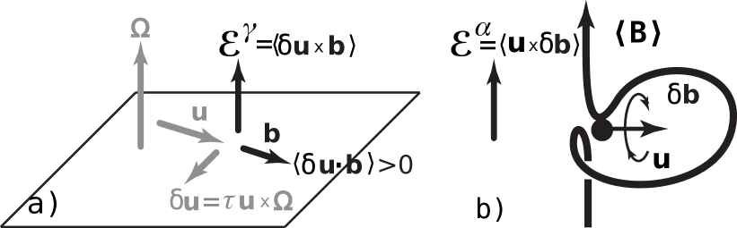
Figure 1: a) Generation of the mean electromotive force from cross-helicity (see explanation in the text); b) the $\alpha$-effect from the axial-aligned magnetic field.

The cross-helicity may have a particular interest for consideration of the dynamo mechanisms operating in the fully-convective stars. For convenience, we briefly remind the physical mechanism behind the cross-helicity generation effect. Illustration of this mechanism is shown in Figure 1a. We consider the aligned turbulent velocity and magnetic field in the plane that is perpendicular to the rotation axis. The Coriolis force acting on the turbulent motion results in the mean electromotive force along the rotation axis, $\boldsymbol{\mathcal{E}}^{\gamma}=\left\langle\delta\mathbf{u}\times\mathbf{b}\right\rangle$ (see, Fig1a). This electromotive force can generate the large-scale toroidal magnetic field due to the $\boldsymbol{\nabla}\times\boldsymbol{\mathcal{E}}^{\gamma}$-term in the induction equation. The alternative mechanism is given by the $\alpha$-effect, (see Figure 1b). In this case, the mean electromotive force results from the large-scale axial magnetic field and the cyclonic motions in the plane perpendicular to the rotation axis. Note that for a regime of the fast rotation the energy of the turbulent vortexes across rotation axis is suppressed. Therefore the axisymmetric $\alpha^{2}$-dynamo cannot use the axial magnetic field for the dynamo generation (Rüdiger & Kitchatinov, 1993). Our consideration gives an idea that the cross-helicity effect can generate the axisymmetric magnetic field even in the case of the quasi 2D turbulence that is expected for the fast-rotating M-dwarfs. The differential rotation of the fast rotating M-dwarfs is rather small (Donati et al., 2008a; Morin et al., 2008). The direct numerical simulations of Browning (2008) show absence of the differential rotation in the magnetic case. Therefore we can expect that the axisymmetric magnetic field is likely generated by means of the turbulent mechanisms with no regards for the large-scale shear flow. As was mentioned above the $\alpha$-effect is unlikely to support the axisymmetric dynamo for the case of the fast-rotating M-dwarfs.

In this paper, the cross-helicity effects are studied for in the full-sphere non-axisymmetric dynamo. We identify the different dynamo scenarios and study the magnetic properties of the fully convective stars using the nonlinear dynamo models.

2 Basic equations

The mean-field convective dynamo is governed by the induction equation of the large-scale magnetic field $\mathbf{B}$,

$$\frac{\partial\mathbf{B}}{\partial t}=\nabla\times\left(\mathbf{\mathcal{E}}+\overline{\boldsymbol{U}}\times\left\langle\mathbf{B}\right\rangle\right),$$ (1)

where $\mathbf{\mathcal{E}}=\left\langle\mathbf{u}\times\mathbf{b}\right\rangle$ is the mean electromotive force of the turbulent convective flows, $\mathbf{u}$, and, the turbulent magnetic field, $\mathbf{b}$. The mean-electromotive force includes the generation effects due to the helical turbulent flows and magnetic field, the generation effect due to the cross-helicity. Also, it includes the turbulent pumping, and the anisotropic (because of rotation) eddy-diffusivity etc.. For convenience, we divide the expression of the mean-electromotive force into two parts:

$$\boldsymbol{\boldsymbol{\mathcal{E}}} = \boldsymbol{\boldsymbol{\mathcal{E}}}^{\alpha,\eta,V}+\boldsymbol{\boldsymbol{\mathcal{E}}}^{\gamma},$$ (2)

where $\boldsymbol{\boldsymbol{\mathcal{E}}}^{\gamma}$ results from the cross-helicity effect (Yokoi, 2013, hereafter Y13):

$$\boldsymbol{\boldsymbol{\mathcal{E}}}^{\gamma}=C_{\gamma}\frac{\boldsymbol{\Omega}}{\Omega}\left\langle\gamma\right\rangle f_{\gamma}\left(\Omega^{*}\right)\psi_{\gamma}\left(\beta\right),$$ (3)

where, $\left\langle\gamma\right\rangle=\left\langle\mathbf{u}\cdot\mathbf{b}\right\rangle$, $\Omega^{*}=4\pi\tau_{c}/P^{*}$ is the Coriolis number, where $\tau_{c}$ is the convective turnover time and the $P^{*}$ is the period of rotation of a star. Analytical calculations of Y13 do not include the nonlinear feedback due to the Coriolis force and the large-scale magnetic field. In our study, these effects will be treated in a simplified way via quenching functions $f_{\gamma}\left(\Omega^{*}\right)$, and $\psi_{\gamma}\left(\beta\right)$. The function $f_{\gamma}\left(\Omega^{*}\right)$ takes into account the nonlinear effect of the Coriolis force in the fast rotation regime. The function $\psi_{\gamma}\left(\beta\right)$, where $\mathrm{\beta=\left\langle\left|\mathbf{B}\right|\right\rangle/\sqrt{4\pi\overline{\rho}u^{\prime 2}}}$, $\mathrm{u^{\prime}}$ is the RMS of the convective velocity, describes the magnetic quenching of the cross-helicity dynamo effect. Those quenching functions will be specified later.

The part $\boldsymbol{\boldsymbol{\mathcal{E}}}^{\alpha,\eta,V}$ includes the others common contributions of the mean-electromotive force. It is written as follows:

$$\boldsymbol{\boldsymbol{\mathcal{E}}}^{\alpha,\eta,V} = \hat{\alpha}\circ\left\langle\mathbf{B}\right\rangle+\mathbf{V}^{\left(p\right)}\times\mathbf{\left\langle B\right\rangle}$$

$$- \left(\eta_{T}+2\eta_{T}^{(\parallel)}\right)\boldsymbol{\nabla}\times\mathbf{\left\langle B\right\rangle}-2\eta_{T}^{(\parallel)}\frac{\boldsymbol{\Omega}}{\Omega^{2}}\mathbf{\boldsymbol{\Omega}\cdot\left(\boldsymbol{\nabla}\times\mathbf{\left\langle B\right\rangle}\right)},$$

It is convenient to divide the large-scale magnetic field induction vector for axisymmetric and non-axisymmetric parts as follows:

$$\left\langle\mathbf{B}\right\rangle = \overline{\mathbf{B}}+\tilde{\mathbf{B}}$$ (5)

$$\mathbf{\overline{B}} = \hat{\boldsymbol{\phi}}\mathrm{B}+\nabla\times\left(\frac{\mathrm{A}\hat{\boldsymbol{\phi}}}{r\sin\theta}\right)$$ (6)

$$\tilde{\mathbf{B}} = \mathrm{\boldsymbol{\nabla}\times\left(\hat{\mathbf{r}}T\right)+\boldsymbol{\nabla}\times\boldsymbol{\nabla}\times\left(\hat{\mathbf{r}}S\right),}$$ (7)

where $\overline{\mathbf{B}}$ is the axisymmetric, and $\tilde{\mathbf{B}}$ is non-axisymmetric part of the large-scale magnetic field; $\mathrm{A}$, $\mathrm{B}$, $\mathrm{T}$ and $\mathrm{S}$ are scalar functions; $\hat{\boldsymbol{\phi}}$ is the unit vector in the azimuthal direction and $\hat{\mathbf{r}}$ is the radius vector; $r$ is the radial distance and $\theta$ is the polar angle. The cross-helicity pseudo-scalar is decomposed to the axisymmetric and non-axisymmetric parts, as well,

$$\left\langle\gamma\right\rangle=\overline{\gamma}+\tilde{\gamma}.$$ (8)

For the non-axisymmetric part of the problem we employ the spherical harmonics decomposition, i.e., the scalar functions $\mathrm{T}$, $\mathrm{S}$ and $\tilde{\gamma}$ are represented as follows:

$$\mathrm{T\left(r,\mu,\phi,t\right)} \mathrm{=} \mathrm{\sum\hat{T}_{l,m}\left(r,t\right)\bar{P}_{l}^{\left|m\right|}\exp\left(im\phi\right),}$$ (9)

$$\mathrm{S\left(r,\mu,\phi,t\right)} \mathrm{=} \mathrm{\sum\hat{S}_{l,m}\left(r,t\right)\bar{P}_{l}^{\left|m\right|}\exp\left(im\phi\right),}$$ (10)

$$\tilde{\gamma}\left(r,\mu,\phi,t\right) = \sum\hat{\gamma}_{l,m}\left(r,t\right)\bar{P}_{l}^{\left|m\right|}\exp\left(im\phi\right)$$ (11)

where $\mathrm{\bar{P}_{l}^{m}}$ is the normalized associated Legendre function of degree $\mathrm{l\geq 1}$ and order $\mathrm{m\geq 1}$. Note that $\mathrm{\hat{S}_{l,-m}=\hat{S}_{l,m}^{*}}$ and the same for $\hat{T}_{l,m}$ and $\hat{\gamma}_{l,m}$.

The equations governing evolution of the axisymmetric part of the magnetic field are as follows:

$$\frac{\partial B}{\partial t} = \frac{1}{r}\left(\frac{\partial r\boldsymbol{\mathcal{E}}_{\theta}^{\alpha,\eta,V}}{\partial r}+\sin\theta\frac{\partial\boldsymbol{\mathcal{E}}_{r}^{\alpha,\eta,V}}{\partial\mu}\right)-\frac{\sin\theta}{r}\frac{\partial\left(\Omega,A\right)}{\partial\left(r,\mu\right)}$$

$$- \frac{1}{r}\left(\frac{\partial r\overline{U}_{r}B}{\partial r}-\sin\theta\frac{\partial\overline{U}_{\theta}B}{\partial\mu}\right)$$

$$- \frac{C_{\gamma}\sin\theta}{r}\left(\frac{\partial}{\partial r}\left(r\left\langle\gamma\psi_{\gamma}\left(\beta\right)\right\rangle f_{\gamma}\left(\Omega^{*}\right)\right)-\frac{\partial}{\partial\mu}\left(\mu\left\langle\gamma\psi_{\gamma}\left(\beta\right)\right\rangle f_{\gamma}\left(\Omega^{*}\right)\right)\right),$$

$$\frac{\partial A}{\partial t} = r\sin\theta\boldsymbol{\mathcal{E}}_{\phi}^{\alpha,\eta,V}-\left(\boldsymbol{\overline{U}}\cdot\boldsymbol{\nabla}\right)A,$$ (13)

where all the parts of the $\boldsymbol{\mathcal{E}}$ except the cross-helicity effect are written in the symbolic form (see, e.g., Yokoi et al. 2016). The Eq(13) does not have a contribution from the cross-helicity. This results in a difference in the cross-helicity dynamo for the axisymmetric and non-axisymmetric magnetic fields. Another important observation is that the cross-helicity dynamo can contribute to generation of the axisymmetric toroidal magnetic field even when the axisymmetric cross-helicity is zero. It results from condition $\overline{\tilde{\gamma}\psi_{\gamma}\left(\beta\right)}\neq 0$ for the nonlinear case in presence of the axisymmetric and non axisymmetric magnetic field.

To get the equation for the functions $\mathrm{S}$ and $\mathrm{T}$ we follow the procedure, which is described in detail by Krause & Rädler (1980). For example, to get the equation for the $\mathrm{S}$ we take the scalar product of the Eq(1) with the $\hat{\mathrm{\boldsymbol{r}}}$ and for the equation governing the $\mathrm{T}$ we do the same after taking the curl of the Eq(1). Therefore we will have,

$$-\frac{\partial\Delta_{\Omega}S}{\partial t} = \boldsymbol{\hat{\mathrm{r}}}\cdot\nabla\times\left(\mathbf{\boldsymbol{\mathcal{E}}}+\overline{\boldsymbol{U}}\times\left\langle\mathbf{B}\right\rangle\right),$$ (14)

$$-\frac{\partial\Delta_{\Omega}T}{\partial t} = \boldsymbol{\hat{\mathrm{r}}}\cdot\nabla\times\nabla\times\left(\boldsymbol{\mathbf{\mathcal{E}}}+\overline{\boldsymbol{U}}\times\left\langle\mathbf{B}\right\rangle\right),$$ (15)

where $1/r^{2}\Delta_{\Omega}$ is the Laplace operator on the surface $r=\mathrm{const}$.

With the contributions of the cross-helicity the Eqs(14,15) are re-written as follows

$$-\frac{\partial\Delta_{\Omega}S}{\partial t} = \boldsymbol{\hat{\mathrm{r}}}\cdot\nabla\times\left(\mathbf{\boldsymbol{\boldsymbol{\mathcal{E}}}^{\alpha,\eta,V}}+\overline{\boldsymbol{U}}\times\left\langle\mathbf{B}\right\rangle\right)+C_{\gamma}f_{\gamma}\left(\Omega^{*}\right)\frac{\partial}{\partial\phi}\left(\tilde{\gamma}\psi_{\gamma}\left(\beta\right)\right),$$ (16)

$$-\frac{\partial\Delta_{\Omega}T}{\partial t} = \boldsymbol{\hat{\mathrm{r}}}\cdot\nabla\times\nabla\times\left(\boldsymbol{\boldsymbol{\mathcal{E}}}^{\alpha,\eta,V}+\overline{\boldsymbol{U}}\times\left\langle\mathbf{B}\right\rangle\right)$$

$$- \frac{C_{\gamma}f_{\gamma}\left(\Omega^{*}\right)}{r}\Delta_{\Omega}\left(\mu\tilde{\gamma}\psi_{\gamma}\left(\beta\right)\right)+\frac{C_{\gamma}}{r}\frac{\partial}{\partial\mu}\left(\sin^{2}\theta\frac{\partial}{\partial r}r\tilde{\gamma}f_{\gamma}\left(\Omega^{*}\right)\psi_{\gamma}\left(\beta\right)\right).$$

We put some details about derivation of Eqs(16, 2) in Appendix. From these equations, we see that the nonaxisymmetric part of the cross-helicity is coupled with the evolution of the non axisymmetric magnetic field. This can provide the dynamo instability of the large-scale non axisymmetric magnetic field. In particular, the nonaxisymmetric magnetic field could be generated solely due to the cross-helicity dynamo effect.

In general case, all coefficients in the Eq(2) depends on the Coriolis number $\Omega^{*}=4\pi\tau_{c}/P^{*}$, where $\tau_{c}$ is the convective turnover time and the $P^{*}$is the period of rotation of a star. Also, the magnetic feedback on the generation and transport effects in the $\boldsymbol{\boldsymbol{\mathcal{E}}}$ should be taken into account. For the case of $\Omega^{*}\gg 1$, the $\alpha$-effect tensor can be represented as follows (Rüdiger & Kitchatinov, 1993; Pipin, 2008):

$$\mathrm{\alpha_{ij}} \mathrm{\approx} \mathrm{c_{\alpha}u^{\prime}\ell\left|\mathbf{\boldsymbol{\Lambda}}^{(\rho)}\right|\cos\theta\psi_{\alpha}(\beta)f_{5}^{(a)}\left(\Omega^{*}\right)\left\{\delta_{ij}-\frac{\Omega_{i}\Omega_{j}}{\Omega^{2}}\right\}}$$ (18)

where, $\mathrm{\mathbf{\boldsymbol{\Lambda}}^{(\rho)}=\boldsymbol{\nabla}\log\overline{\rho}}$ is the gradient of the mean density. Although, $f_{5}^{(a)}\left(\Omega^{*}\right)\rightarrow\pi/2$, when $\Omega^{*}\gg 1$, we will keep the dependence on the Coriolis number for the nonlinear solution. For the case $\Omega^{*}\gg 1$, the magnitude of the kinetic part $\alpha$ effect is given by

$$\alpha_{0}={\displaystyle\frac{\pi}{2}c_{\alpha}u^{\prime}\ell\left|\mathbf{\boldsymbol{\Lambda}}^{(\rho)}\right|}.$$ (19)

The magnetic quenching function of the kinetic part of $\alpha$-effect is defined by

$$\psi_{\alpha}=\frac{5}{128\beta^{4}}\left(16\beta^{2}-3-3\left(4\beta^{2}-1\right)\frac{\arctan\left(2\beta\right)}{2\beta}\right),$$ (20)

where $\mathrm{\beta=\left\langle\left|\mathbf{B}\right|\right\rangle/\sqrt{4\pi\overline{\rho}u^{\prime 2}}}$. For the cross-helicity dynamo effect we assume that $\psi_{\gamma}=\psi_{\alpha}$. For the sake of simplicity, we skip the magnetic quenching due to the magnetic helicity conservation, (cf, Pipin et al. 2013).

The turbulent pumping of the mean-field contains the sum of the contributions due to the mean density gradient (see,Pipin, 2008, hereafter P08) and the mean-filed magnetic buoyancy (Kitchatinov & Pipin, 1993),

$$\mathbf{V}^{\left(p\right)}\times\mathbf{\left\langle B\right\rangle} \mathrm{=} 3\eta_{0}f_{1}^{(a)}\left(\Omega^{*}\right)\left(\frac{\left(\Omega\cdot\boldsymbol{\Lambda}^{(\rho)}\right)}{\Omega^{2}}\boldsymbol{\Omega}\times\mathbf{\left\langle B\right\rangle}-\left(\boldsymbol{\Omega}\cdot\mathbf{\left\langle B\right\rangle}\right)\left(\boldsymbol{\Omega}\times\boldsymbol{\Lambda}^{(\rho)}\right)\right)$$

$$+ \frac{\alpha_{MLT}u^{\prime}}{\Gamma_{1}}\beta^{2}K\left(\beta\right)\mathrm{\mathbf{g}}\times\mathbf{\left\langle B\right\rangle}$$

where the $\mathrm{\alpha_{MLT}}$ is the parameter of the mixing length theory, $\Gamma_{1}$ is the adiabatic exponent and the function $\mathrm{K\left(\beta\right)}$ is defined in (Kitchatinov & Pipin, 1993) and $\mathbf{g}$ is the unit vector in the radial direction. When $\Omega^{*}\gg 1$, we have $f_{1}^{(a)}\left(\Omega^{*}\right)\rightarrow\pi/(8\Omega^{\ast})$. The function of the Coriolis number $f_{1}^{(a)}\left(\Omega^{*}\right)$ is given in P08. Dependence of the eddy-diffusivity coefficients on the Coriolis number is as follows

$$\eta_{T} = \frac{\eta_{0}}{\Omega^{*2}}\left(1-\frac{\arctan\Omega^{*}}{\Omega^{*}}\right)$$

$$\eta_{T}^{\|} = \frac{3\eta_{0}}{4\Omega^{*2}}\left(\left(\Omega^{*2}+3\right)\frac{\arctan\Omega^{*}}{\Omega^{*}}-3\right),$$

where the eddy-diffusivity coefficient is defined ${\displaystyle\eta_{0}=\mathrm{\nu_{0}/Pm_{T}}}$ where $\nu_{0}=\mathrm{u}^{\prime}\ell/3$ is the eddy viscosity.

The quenching of the cross-helicity dynamo for the fast rotating case was not studied before. We will assume that the cross-helicity effect is quenched in the same way as the turbulent diffusivity coefficients, i.e., we put

$$f_{\gamma}\left(\Omega^{*}\right)=\frac{1}{\pi}\frac{\arctan\Omega^{*}}{1+\Omega^{*}}$$ (22)

The Eq(22) affect the amplitude of the cross-helicity effect in the large-scale dynamo.

The evolution of the cross-helicity is govern by the conservation law

$$\frac{\partial\left\langle\gamma\right\rangle}{\partial t}=\frac{1}{3\overline{\rho}}\left(\left\langle\mathbf{B}\right\rangle\cdot\nabla\right)\overline{\rho}\left\langle\mathbf{u}^{2}\right\rangle-2\boldsymbol{\boldsymbol{\mathcal{E}}}\cdot\boldsymbol{\Omega}+\eta_{0}\Delta\left\langle\gamma\right\rangle$$ (23)

In the stellar conditions, the typical spatial scale of the density stratification is much less than the spatial scale of the mean magnetic field. Thus, the first term in the Eq(23) dominates the second one. Either rotation-induced anisotropy of the $\alpha$-effect, the eddy diffusivity, and the pumping do not contribute to the cross-helicity generation. Substituting the general expression of the mean-electromotive force into Eq(23) we get,

$$\frac{\partial\left\langle\gamma\right\rangle}{\partial t}=\frac{\eta_{0}}{\tau_{c}}\left(\left\langle\mathbf{B}\right\rangle\cdot\boldsymbol{\Lambda}^{(\rho)}\right)+2\eta_{T}\boldsymbol{\Omega}\cdot\left(\boldsymbol{\nabla}\times\mathbf{\left\langle B\right\rangle}\right)-\frac{\Omega\alpha_{MLT}u^{\prime}}{\Gamma_{1}}\beta^{2}K\left(\beta\right)\sin\theta\left\langle B_{\phi}\right\rangle+\eta_{0}\Delta\gamma,$$ (24)

For the numerical solution, we reduce the equations to the dimensionless form. The radial distance is measured in the units of the solar radius, as usual for the stellar astrophysics. Thus, we will have the following set of parameters, the $\Omega_{\star}$ is the rotation rate of the star, the $\nu_{0}$ is the magnitude of the eddy viscosity, the parameter $\mathrm{Pm_{T}}$.

The boundary conditions are as follows. The cross-helicity and magnetic field are put to zero at the inner boundary which is close to the center of the star. For the top, we use the vacuum boundary conditions for the magnetic field. The boundary condition for the cross-helicity at the top is unknown, we put the radial derivative to zero at the top.

2.1 The possible dynamo scenarios

The possible dynamo scenarios depend upon the magnetic field generation mechanisms, such as the $\alpha$-effect, the so-called $\Omega$-effect (associating with the differential rotation) and the cross-helicity dynamo effect (denoted as the $\gamma$-effect). Following conventions of the dynamo theory (Krause & Rädler, 1980), we can identify the following scenarios: $\alpha^{2}$, $\alpha^{2}\Omega$, $\gamma^{2}$, $\gamma^{2}\Omega$, $\alpha^{2}\gamma^{2}$, and $\alpha^{2}\gamma^{2}\Omega$. More scenarios can be found in Krause & Rädler (1980). From the point of view of this study, the scenarios of $\gamma^{2}$ , $\alpha^{2}\gamma^{2}$, and $\alpha^{2}\gamma^{2}\Omega$ present particular interest. All of them depend on the cross-helicity generation governed by the Eq(24).

The conceivable scenarios of the cross-helicity dynamos depend on the cross-helicity generation effect. The simplest scenario realized when the cross-helicity is generated from the axial current, e.g., the term $2\eta_{T}\boldsymbol{\Omega}\cdot\left(\boldsymbol{\nabla}\times\mathbf{\left\langle B\right\rangle}\right)$ in the RHS of the Eq(24). If we consider the axisymmetric magnetic field, $\gamma^{2}$ dynamo can give generation of the toroidal magnetic field from the cross-helicity effect. The poloidal field is decoupled from the system of the dynamo equation and it can have only a decaying solution. This scenario was discussed previously by Yoshizawa & Yokoi (1993) and Yokoi (2013) for the dynamo in accretion disks.

In stellar convection zone, the cross-helicity generation due to the density stratification is one of the most important mechanism. This is supported by the direct numerical simulations of Matthaeus et al. (2008). This effect is accounted by the first term in the cross-helicity evolution equation. With regards to the density stratification, all the dynamo equations are coupled and there is a possibility for $\gamma^{2}$ dynamo. In this case, only the non-axisymmetric modes can be unstable in linear solution because the mean electromotive force $\boldsymbol{\boldsymbol{\mathcal{E}}}=\dots+C_{\gamma}\left\langle\gamma\right\rangle\tau_{c}\boldsymbol{\Omega}+\dots$ has no contribution in the equation for the axisymmetric poloidal magnetic field (associated with the potential A). In what follows we discuss $\gamma^{2}$ , $\alpha^{2}\gamma^{2}$, and $\alpha^{2}\gamma^{2}\Omega$ scenarios based on the cross-helicity generation effect which comes from the first term of the Eq(24).

3 Results

3.1 The eigenvalue problem

For the linear eigenvalue problem we consider the simplified set of the equations. We assume that the eddy diffusivity, $\eta_{0}=\nu_{0}/\mathrm{Pm_{T}}$ with $\nu_{0}=5\cdot 10^{10}\mathrm{cm^{2}}$/s is constant over radial distance. This corresponds to set of parameters in our model for the $0.3\mathrm{M}_{\odot}$ star rotating with the period of 10 days. The density gradient scale has sharp variation in the upper part of the star and it is nearly constant in depth. It was found that it is important to keep the spatial variations of the $\mathbf{\boldsymbol{\Lambda}}_{r}^{(\rho)}$ for the for the cross-helicity evolution equation. For the eigenvalue problem we introduce a new variable, $\xi=R_{\odot}\mathbf{\boldsymbol{\Lambda}}_{r}^{(\rho)}$, and employ the adiabatic profile of the density variation scale,

$$\xi\left(r\right)=\frac{1}{2}R_{\star}R_{\odot}/\left(r\left(R_{\star}-r\right)\right).$$ (25)

Parameter $\xi$ is nearly uniform in the bulk of the star, having $\xi\approx-10$ and it rapidly falls to $\xi\approx-500$ toward the surface. For the sake of simplicity, we put the constant $\xi=-50$ in the pumping terms. The amplitude of the $\alpha$-effect will be determined by parameter $C_{\alpha}={\displaystyle\alpha_{0}R_{\odot}/\nu_{0}}$. Additional parameter is the ratio $C_{\tau}={\displaystyle R_{\odot}^{2}/\left(\nu_{0}\tau_{c}\right)}$. It determines the generation of the cross-helicity. Therefore, in the linear problem, the reduced expression of the mean-electromotive force is

$$\hat{\mathcal{E}}_{i} = \mathrm{C_{\alpha}\mathrm{Pm_{T}^{-1}}\left\{\left\langle B_{i}\right\rangle-\frac{\Omega_{i}\left(\boldsymbol{\Omega}\cdot\left\langle\mathbf{B}\right\rangle\right)}{\Omega^{2}}\right\}}+C_{h}\hat{\gamma}$$

$$+\mathrm{Pm_{T}^{-1}}\left(\frac{\left(\Omega\cdot\boldsymbol{\xi}\right)}{\Omega^{2}}\boldsymbol{\Omega}\times\mathbf{\left\langle B\right\rangle}-\left(\boldsymbol{\Omega}\cdot\mathbf{\left\langle B\right\rangle}\right)\left(\boldsymbol{\Omega}\times\boldsymbol{\xi}\right)\right),$$

$$- \mathrm{Pm_{T}^{-1}}\left(\left(1+2a\right)\boldsymbol{\nabla}\times\mathbf{\left\langle B\right\rangle}+2a\frac{\boldsymbol{\Omega}}{\Omega^{2}}\mathbf{\boldsymbol{\Omega}\cdot\left(\boldsymbol{\nabla}\times\mathbf{\left\langle B\right\rangle}\right)}\right),$$

where $a=\eta_{T}^{\|}/\eta_{T}$. In what follows we assume that $a=1$. Also, in the linear problem the parameter $C_{h}=C_{\gamma}\Omega_{\star}\tau_{c}$ in the Eq(3.1) absorbs the Coriolis number dependence. The hat sign in Eq(3.1) means that the mean electromotive force was scaled about $\nu_{0}$. The cross-helicity is governed by equation

$$\frac{\partial\hat{\gamma}}{\partial t}=C_{\tau}\mathrm{Pm_{T}^{-1}}\left(\left\langle\mathbf{B}\right\rangle\cdot\boldsymbol{\xi}\right)+\mathrm{Pm_{T}^{-1}}\Delta\hat{\gamma},$$ (27)

Our purpose to investigate the eigenvalue solution of the Eqs(1,3.1,27) for the set of parameters like $\mathrm{Pm_{T}}$ $C_{\alpha}$, $C_{\gamma}$, and $C_{\tau}$. The effect of the differential rotation can be controlled by the angular velocity of the star and the distribution of the differential rotation. We put $C_{\tau}=100$ because the typical diffusive time scale is order of 100 years and the $\tau_{c}\approx 1$ year for this star. For the external layers of the star, the $C_{\tau}$ is much larger. We consider the profile of the differential rotation from our previous paper (Pipin, 2017). It is illustrated in Figure 2.

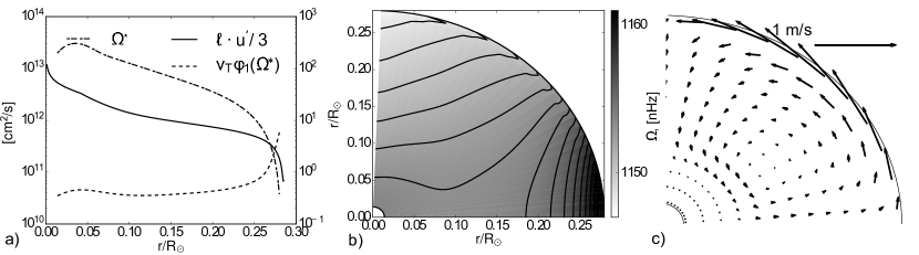
Figure 2: a) The Coriolis number $\Omega^{*}=2\tau_{c}\Omega_{\star}$ (dash-dot line), where $\tau_{c}$ is the turn-over time of convection, the turbulent diffusivity parameter, solid line, both the $\tau_{c}$ and the diffusivity are estimated from the MESA code; the dashed line shows the isotropic eddy viscosity from the heat transport model; b) angular velocity profiles with contour levels which cover the range of values which are depicted on the grey scale bar; c) geometry of the meridional circulation, in the Northern hemisphere.

In linear solution, all the partial dynamo modes are decoupled. We restrict discussion to a few partial modes of the large-scale magnetic field, including the axisymmetric modes S0 and A0 and the non-axisymmetric modes S1 and A1. We follow convention suggested by Krause & Rädler (1980): the letter “S” means the mode symmetrical about equator and the letter “A” is for the antisymmetric mode.

With no regards for the cross-helicity dynamo effect, e.g., in case of $C_{\tau}=0$ or $C_{h}=0$ , the large-scale dynamo instability is provided by the $\alpha^{2}$ or $\alpha^{2}\Omega$ scenarios. For the $\alpha^{2}$ scenario, the critical $C_{\alpha}$ does not depend on $\mathrm{Pm_{T}}$. Also, in this scenario, the non-axisymmetric modes are preferable having thresholds at $C_{\alpha}^{(cr)}\approx 37$ for the A1 mode and at $C_{\alpha}^{(cr)}\approx 42$ for the S1 mode and for $a=0$. The thresholds are about factor one-half higher for $a=1$ than for $a=0$. This means that the additional diffusive mixing of the large-scale magnetic field quenches efficiency of the dynamo mechanisms. In $\alpha^{2}\Omega$ dynamo the instability depends largely on parameter Pm, because this parameter controls the efficiency of the large-scale magnetic field stretching by the differential rotation. For the $\mathrm{Pm_{T}}$=20, the axisymmetric modes are unstable first, having thresholds around $C_{\alpha}^{(cr)}\approx 10$.

The cross-helicity generation effect adds the new parameters for the study. Results are shown in Figures 3a and b. We restrict the study by fixing the $C_{\alpha}$ parameter below the dynamo thresholds of $\alpha^{2}$ and $\alpha^{2}\Omega$ dynamo regimes. We put the $C_{\alpha}=10$ and the anisotropy parameter $a=0$, and study the dynamo instability against the parameter $C_{h}$ for the variable magnetic Prandtl number $\mathrm{Pm_{T}}$ . Figures 3a shows results for the pure turbulent dynamo scenarios, i.e., the differential rotation is disregarded. It is found that the mode A1 keeps the least dynamo threshold. Also, we found the $\gamma^{2}$ scenario has the smaller dynamo instability thresholds for modes A1 and S1 than the $\alpha^{2}\gamma^{2}$ scenario. Therefore we can conclude that the magnetic field generation by the concurrent cross-helicity and $\alpha^{2}$ dynamos reduce the efficiency of both dynamo mechanisms. The results of the linear analysis tells us that without the differential rotation the nonaxisymmetric dynamo solution is preferable. We can conclude that during the linear stage of the dynamo process the $\gamma^{2}$ scenario does not give any preference for the axisymmetric magnetic field generation. Moreover, as it was anticipated from the dynamo equations the $\gamma^{2}$ scenario provide the additional mechanisms for the non-axisymmetric magnetic field generation.

Figure 3: a) Excitation thresholds for $\alpha^{2}\gamma^{2}$ scenario (red lines for the A-modes and blue lines for the S-modes) and $\gamma^{2}$-scenario (black lines, the dashed line is for the A1 mode and the solid line is for S1-mode) dynamos; b) the same as (a) for the $\alpha^{2}\Omega\gamma^{2}$ dynamos. The $\alpha$-effect parameter $C_{\alpha}=10$.

Figure 2b shows that with an account of the differential rotation effect, i.e., in considering the $\alpha^{2}\Omega\gamma^{2}$ dynamo scenario, we get the instability thresholds for all the modes close to each other with an increase of $\mathrm{Pm_{T}}$. Also, the efficiency of the axisymmetric dynamo instability increases with the increase of $\mathrm{Pm_{T}}$. Within the studied parameter range of $\mathrm{Pm_{T}}$ the nonaxisymmetric mode A1 keeps to be the most unstable. We also studied instability for the spatially nonuniform density stratification parameter $\xi$. In this case the dynamo instability thresholds are about a factor of magnitude larger than in the case of the constant $\xi$. However, the order of the instability thresholds among the different partial dynamo modes remains the same as it is shown in Figures 3a and b.

3.2 The nonlinear solution

For the nonlinear solution, we employ the model which keeps the spatial dependence of the turbulent parameters provided by the MESA code and solution of the heat transport problem (see Pipin 2017). Using the results of the eigenvalue problem we bear in mind that the parameters $C_{h}$ and $C_{\tau}$ in the Eqs(3.1) and (27) absorb the dependence upon the parameter $\tau_{c}$. It is found that the Coriolis number parameter $\Omega^{*}=4\pi\tau_{c}/P^{*}$, where $P^{*}=10$ days, varies from about 1 near the surface to 200 in the depth of the star. This means that the critical threshold of the $C_{\gamma}=2C_{h}/\Omega^{*}\ll 1\sim 0.01$ for $\alpha^{2}\Omega\gamma^{2}$ dynamo if $\mathrm{Pm_{T}}=3$. We use this $\mathrm{Pm_{T}}$ in all models below. Three different models will be considered. Parameters of the models are listed in Table 1. The model M1 represent the $\gamma^{2}$ scenario, the model M2 represents the $\alpha^{2}\gamma^{2}$ scenario and M3 stands for $\alpha^{2}\tilde{\gamma}^{2}$. In the latter case, we disregard the contribution of the axisymmetric cross-helicity in the mean-electromotive force. This imitates the situation when the mean cross-helicity has no hemispheric sign rule. The nonlinear combination of the nonaxisymmetric magnetic field and cross helicity can produce the axisymmetric magnetic field. The model M3 was introduced to study this situation. In this paper, we consider models with the solid body rotation.

Table 1:

Model	Scenario	$C_{\gamma}$	$C_{\alpha}$
M1	$\gamma^{2}$	0.01
M2	$\alpha^{2}\gamma^{2}$	0.01	0.03
M3	$\alpha^{2}\tilde{\gamma}^{2}$	0.01	0.03

Regime $\gamma^{2}$ provides the simplest scenario of the cross-helicity dynamo. Contrary to the $\alpha^{2}$ dynamo, the $\gamma^{2}$ works only in the nonaxisymmetric regime. In this scenario evolution of the axisymmetric components of the toroidal and poloidal magnetic fields are decoupled. Figures 4 and 5 show evolution of the partial modes in the model M1 as well as snapshots of the magnetic field and the cross-helicity distributions at the stationary stage of evolution. It is seen that the axisymmetric mode of the toroidal magnetic field evolves non-monotonically showing growth at the beginning and it decays afterwhile. In nonlinear case, the cross-helicity that is produced by the non-axisymmetric magnetic field may contribute to generation of the axisymmetric toroidal magnetic field, because in general $\left\langle\gamma\psi_{\gamma}\left(\beta\right)\right\rangle\neq 0$ (see, eq.2). Therefore, the nonaxisymmetric cross-helicity affects generation of the axisymmetric toroidal magnetic field. However, evolution of the axisymmetric poloidal magnetic field is decoupled of the toroidal magnetic field and the axisymmetric cross-helicity. Therefore, there is no true axisymmetric dynamo in this case. The axisymmetric field starts to decay when parts of the product $\left\langle\gamma\psi_{\gamma}\left(\beta\right)\right\rangle$ get synchronized. Both the non-axisymmetric cross-helicity density $\gamma$ and magnetic field can be represented by the equatorial dipole which changes orientation rotating around the axis of stellar rotation. This phenomenon is known as the nonaxisymmetric dynamo waves.

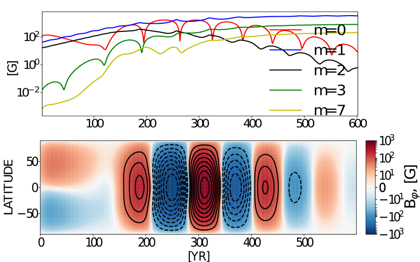
Figure 4: The model M1 ( $\gamma^{2}$ dynamo), a) shows evolution of the partial modes of the toroidal magnetic field at at the $\mathrm{r=\frac{3}{4}R_{\star}}$; b) the time-latitude diagram of the toroidal magnetic field shown by the color image and contours (range of $\pm$1kG).

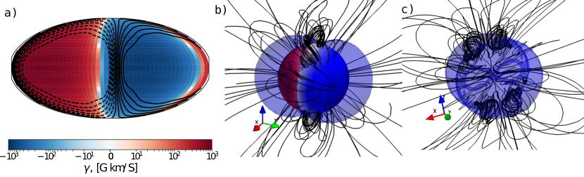
Figure 5: The model M1, snapshots of the cross-helicity and magnetic field distributions in the stationary phase of dynamo evolution, a) the cross-helicity distributions is shown by color and the radial magnetic field (iso-lines $\pm 1$kG); b) strength of the toroidal magnetic field at the $\mathrm{r=\frac{3}{4}R_{\star}}$ for axisymmetric and non-axisymmetric magnetic field and the ratio between energy of the axisymmetric magnetic field and total magnetic energy; b) the time-latitude diagram for axisymmetric toroidal magnetic field at the $\mathrm{r=\frac{3}{4}R_{\star}}$and the color image shows shows the axisymmetric radial magnetic field at the surface.

The scenario of the $\alpha^{2}\gamma^{2}$ dynamo has a possibility for the axisymmetric magnetic field generation. Figures 6 and 7 show evolution of the partial modes in the model M2 as well as snapshots of the magnetic field and the cross-helicity distributions at the stationary stage of evolution. We use the output of the model M1 as an initial condition for the model M2. The Figs.6(a) and (b) show that the axisymmetric toroidal magnetic field started to grow at the beginning phase showing some oscillations. The dynamo solution reaches the stage with the constant dipole-like distribution at the end of simulation. The similar behavior is demonstrated by the cross-helicity evolution. The cross-helicity has the opposite signs in the northern and southern hemispheres. The polar magnetic field in model M2 reaches a magnitude of the 2kG. At the end of simulation, the model keeps a substantial nonaxisymmetric magnetic field. It has more than one order of magnitude less strength than the axisymmetric magnetic field. Snapshots of the magnetic field and cross-helicity distributions show that these nonaxisymmetric components concentrate in the near equatorial regions. The field lines of the magnetic field distribution show that the overall configuration of the magnetic field is dipole-like both inside and outside the star.

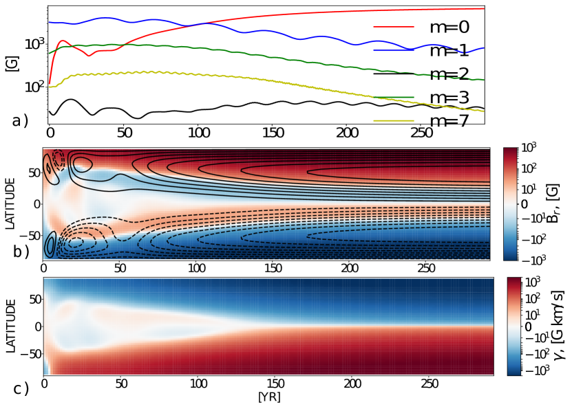
Figure 6: The model M2 ($\alpha^{2}\gamma^{2}$ dynamo) a) shows evolution of the partial modes of the toroidal magnetic field at at the $\mathrm{r=\frac{3}{4}R_{\star}}$; b) time-latitude diagram of the radial magnetic field at the surface shown by the color image and contours show the toroidal magnetic field at at the $\mathrm{r=\frac{3}{4}R_{\star}}$ (range of $\pm$3kG); c) shows the time-latitude evolution for the cross-helicity

Using the output of the model M2 we made additional run neglecting the cross-helicity generation effects. This return the dynamo model to the $\alpha^{2}$ scenario. Similar to Pipin (2017) we get the non-axisymmetric magnetic field at the end of the run. Also, we made additional runs with the decreased $C_{\gamma}$. For the given parameter $C_{\alpha}$ it was found that the model keeps axisymmetric magnetic even in the case when $C_{\gamma}$ is by a factor 2 less than in the model M2.

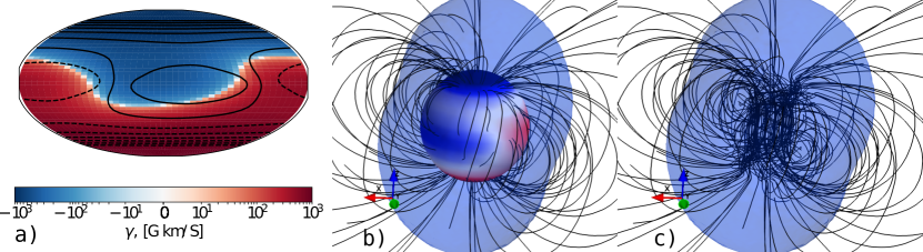
Figure 7: The same as Fig.5 for the model M2.

The interesting question is if the axisymmetric dynamo can be sustained by the cross-helicity generation effect when the spatially averaged cross-helicity is zero. The model M3 illustrates this scenario. In this model, we disregard the contribution of the axisymmetric cross-helicity in the mean-electromotive force by neglecting contributions of the axisymmetric magnetic field in the equation of the cross-helicity evolution. Results are shown in Figures 8 and 9. Results show that contrary to the pure $\gamma^{2}$ scenario the axisymmetric magnetic field is generated. This means that the azimuthally averaged cross-helicity dynamo effect is not zero, $\left\langle\gamma\psi_{\gamma}\left(\beta\right)\right\rangle\neq 0$, because the terms of the product $\left\langle\gamma\psi_{\gamma}\left(\beta\right)\right\rangle$ are not synchronized in the azimuthal direction. It is caused by the nonlinear generation of the non axisymmetric magnetic field both by the $\gamma^{2}$ and the $\alpha^{2}$ mechanisms. We see that the strength of the axisymmetric and nonaxisymmetric toroidal magnetic field is same by the order of magnitude. The axisymmetric magnetic field shows the solar-like time-latitude evolution of the toroidal magnetic field inside the star. The radial magnetic field at the surface shows the dominant nonaxisymmetric magnetic field and the nonaxisymmetric distribution of the cross-helicity. During the nonlinear evolution the pattern of the magnetic field distribution shown in Fig. 9b moves about the axis of rotation, representing the azimuthal dynamo wave. Also, it weakly oscillates around the perpendicular axis which corresponds to the axis of the equatorial dipole. By this reason, the model can show the nearly axisymmetric configuration of the polar magnetic field during the minims and maxims of the axisymmetric magnetic field cycle. The frequency of the non-axisymmetric m=1 mode is twice of the axisymmetric one.

4 Discussion and conclusions

The physical origin of this cross-helicity effect lies in the combination of the local angular-momentum conservation in a rotational motion and the presence of the velocity-magnetic-field correlation (Yokoi, 2013). Unlike the $\Omega$ effect, the cross-helicity effect does not depend on the particular configuration of the differential rotation. Provided that a finite turbulent cross helicity exists, the cross-helicity effect should work in the presence of the absolute vorticity (rotation and relative vorticity). This means that we can expect the cross-helicity dynamo mechanism to work even in the case that the differential rotation is negligibly small. How and how much cross helicity exists in turbulence is another problem. In our models, the turbulent cross helicity is generated by means of the large-scale magnetic field and density stratification. This generation mechanism was analytically found in a number of papers (Yokoi, 1999; Pipin et al., 2011; Rüdiger et al., 2011; Yokoi, 2013) using the mean-field magnetohydrodynamics framework. Our results show that this turbulent cross-helicity generation effect results in a number of the new dynamo scenarios.

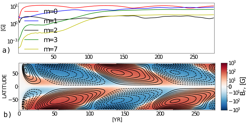
Figure 8: The $\alpha^{2}\tilde{\gamma}^{2}$ dynamo, a) shows evolution of the partial modes of the toroidal magnetic field at at the $\mathrm{r=\frac{3}{4}R_{\star}}$; b) time-latitude diagram of the radial magnetic field at the surface shown by the color image and contours show the toroidal magnetic field at at the $\mathrm{r=\frac{3}{4}R_{\star}}$ (range of $\pm$3kG).

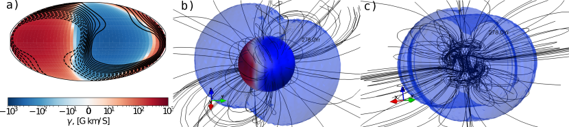
Figure 9: The same as Fig.5 for the model M3.

It was shown that for the solid body rotation regime there are three possible dynamo scenarios: the $\gamma^{2}$-dynamo (pure cross-helicity dynamo), the $\alpha^{2}\gamma^{2}$-dynamo and its modification - the $\alpha^{2}\tilde{\gamma}^{2}$ dynamo. The latter is operating from the purely nonaxisymmetric cross-helicity distribution. In nonlinear case, both the $\gamma^{2}$ and the $\alpha^{2}$ dynamo scenarios sustain only the nonaxisymmetric magnetic field. For the $\gamma^{2}$ scenario the evolution axisymmetric components of the magnetic field are decoupled. Therefore this regime cannot sustain the axisymmetric magnetic field against decay.

An interesting new effect was considered. It is found that, in general, it is possible to generate some axisymmetric magnetic field in nonlinear regime if the spatial variations of the non-axisymmetric distributions of the cross-helicity and magnetic energy are not synchronized in the azimuthal direction. This gives generation of the axisymmetric toroidal magnetic field due to the cross-helicity dynamo effect because for the axisymmetric part of $\left\langle\gamma\psi_{\gamma}\left(\beta\right)\right\rangle$ we have

$$\left\langle\gamma\psi_{\gamma}\left(\beta\right)\right\rangle=\overline{\gamma}\overline{\psi_{\gamma}\left(\beta\right)}+\overline{\tilde{\gamma}\tilde{\psi_{\gamma}\left(\beta\right)}}\neq 0,$$ (28)

where the first term of RHS is zero in $\gamma^{2}$ regime. The second term of the RHS of this equation is not necessarily zero. Results of the model M1 show that in the $\gamma^{2}$ scenario the $\tilde{\gamma}$ and $\tilde{\psi_{\gamma}\left(\beta\right)}$ get synchronized. This prevents the axisymmetric toroidal magnetic field generation. On the other hand, if there is an additional mechanism of the nonaxisymmetric magnetic field generation, e.g. by the $\alpha^{2}$ dynamo, then the axisymmetric dynamo can be excited even if the axisymmetric part of the cross-helicity is zero. This was demonstrated by model M3 using the $\alpha^{2}\tilde{\gamma}^{2}$ scenario. There, the effect of the axisymmetric cross-helicity generation was disregarded. The given mechanism shows a mixture of the non-axisymmetric and axisymmetric modes with a dominance of the equatorial dipole-like mode.

One of the most important findings of our work is that the axisymmetric magnetic field can be generated by means of the cross-helicity generation and $\alpha^{2}$ in this case we employ the standard formulation of the mean-electromotive force suggested by Yoshizawa et al. (2000). The dynamo mechanism operates with regards to the axisymmetric and non-axisymmetric cross-helicity generation. In this case, the strong axisymmetric dipole-like magnetic field is generated. Unlike the nonlinear $\alpha^{2}\Omega$ regimes (cf. Pipin, 2017), this scenario produces the constant in time magnetic field configuration with antisymmetric about equator cross-helicity, toroidal and radial magnetic field distributions. Our scenario was demonstrated for the solid body regime. This means that it can be realized on the fast rotating M-dwarfs with a period of rotation about 1day, which often show only a small amount of the differential rotation (Donati et al., 2008a). Moreover the direct numerical simulation e.g., Browning (2008), and mean-field models, e.g., Pipin (2017) show suppression of the differential rotation in nonlinear regimes. For the solid body rotation, $\alpha^{2}$ dynamo produce the nonaxisymmetric magnetic field (Chabrier & Küker, 2006; Elstner & Rüdiger, 2007). This because the $\alpha$-effect cannot use the component of the large-scale magnetic field along rotation for generation the axial electromotive force and this results from the anisotropic $\alpha$-effect in the case of the high Coriolis number (see, Eq18 and Rüdiger & Kitchatinov, 1993). The cross-helicity can generate the poloidal electromotive force in this case (Yokoi, 2013). This provides generation of the axisymmetric magnetic field by the $\alpha^{2}\gamma^{2}$-dynamo. The magnetic field configuration produced in our model of $\alpha^{2}\gamma^{2}$-dynamo is very similar to those which was found on the fast rotating M-dwarfs, e.g., V374 Peg and YZ CMi (Donati et al., 2008b, a; Donati & Landstreet, 2009).

In our paper we employ rather simplified approach to model the cross-helicity generation effects for the fast rotating regimes. For the further application the analytical results for the cross-helicity generation effect in case of the fast rotation and strong magnetic field have to be developed. We hope that future work could shed more light about usability of the cross-helicity generation effects in stellar dynamos.

Acknowledgments We thank support RFBR under grant 16-52-50077. Valery Pipin thank the grant of Visiting Scholar Program supported by the Research Coordination Committee, National Astronomical Observatory of Japan (NAOJ) and the project II.16.3.1 of ISTP SB RAS.

5 Appendix

To derive evolution equations for the non-axisymmetric parts of the magnetic field we use approach suggested by Krause & Rädler (1980) and some useful identities (more of them can be found in their book). For any scalar functions T and S and radius vector $\hat{\mathbf{r}}$ we have:

$$\boldsymbol{\nabla}\times\left(\hat{\mathbf{r}}T\right) = -\hat{\mathbf{r}}\times\boldsymbol{\nabla}T$$

$$\boldsymbol{\nabla}\times\boldsymbol{\nabla}\times\left(\hat{\mathbf{r}}S\right) = \boldsymbol{\nabla}\frac{\partial rS}{\partial r}-r\Delta S,$$

$$\boldsymbol{\hat{\mathbf{r}}\cdot\nabla}\times\boldsymbol{\nabla}\times\left(\hat{\mathbf{r}}S\right) = -\Delta_{\Omega}S$$

$$= -\frac{1}{\sin\theta}\frac{\partial}{\partial\theta}\left(\sin\theta\frac{\partial S}{\partial\theta}\right)-\frac{1}{\sin^{2}\theta}\frac{\partial^{2}S}{\partial\phi^{2}}$$

To derive Eq(14), we substitute $\boldsymbol{\mathbf{B}}=\hat{\boldsymbol{\phi}}\mathrm{B}+\nabla\times\left(\frac{\mathrm{A}\hat{\boldsymbol{\phi}}}{r\sin\theta}\right)+\boldsymbol{\nabla}\times\left(\hat{\mathbf{r}}T\right)+\boldsymbol{\nabla}\times\boldsymbol{\nabla}\times\left(\hat{\mathbf{r}}S\right)$ to the LHS of the Eq(1) and taking into account nonaxisymmetry and the Eq(5) we get ${\displaystyle\frac{\partial\left(\hat{\mathbf{r}}\cdot\boldsymbol{\mathbf{B}}\right)}{\partial t}=-\frac{\partial\Delta_{\Omega}S}{\partial t}}$. For the cross-helicity contribution to the RHS of that equation we have:

$$\boldsymbol{\hat{\mathrm{r}}}\cdot\nabla\times\left(\mathbf{\boldsymbol{\mathcal{E}}}^{\gamma}\right) = C_{\gamma}\boldsymbol{\hat{\mathrm{r}}}\cdot\nabla\times\left(\frac{\boldsymbol{\Omega}}{\Omega}\left\langle\gamma\right\rangle f_{\gamma}\left(\Omega^{*}\right)\psi_{\gamma}\left(\beta\right)\right)$$

$$= C_{\gamma}\boldsymbol{\hat{\mathrm{r}}}\cdot\nabla\times\left(\left(\frac{\boldsymbol{\hat{\mathrm{r}}}}{r}\mu-\hat{\theta}\sin\theta\right)\left\langle\gamma\right\rangle f_{\gamma}\left(\Omega^{*}\right)\psi_{\gamma}\left(\beta\right)\right)$$

$$= C_{\gamma}\nabla\cdot\left(\boldsymbol{\hat{\mathrm{r}}}\times\hat{\theta}\right)\sin\theta\left\langle\gamma\right\rangle f_{\gamma}\left(\Omega^{*}\right)\psi_{\gamma}\left(\beta\right)$$

$$= C_{\gamma}\frac{\partial}{\partial\phi}\left\langle\gamma\right\rangle f_{\gamma}\left(\Omega^{*}\right)\psi_{\gamma}\left(\beta\right),$$

where $\hat{\theta}$ is the unit vector along polar angle coordinate.

References

- Berdyugina (2005) Berdyugina, S. V. 2005, Living Reviews in Solar Physics, 2, 8
- Birch (2011) Birch, A. C. 2011, Journal of Physics Conference Series, 271, 012001
- Brandenburg & Subramanian (2005) Brandenburg, A., & Subramanian, K. 2005, Phys. Rep., 417, 1
- Brown et al. (2011) Brown, B. P., Browning, M. K., Brun, A. S., Miesch, M. S., & Toomre, J. 2011, in Astronomical Society of the Pacific Conference Series, Vol. 448, 16th Cambridge Workshop on Cool Stars, Stellar Systems, and the Sun, ed. C. Johns-Krull, M. K. Browning, & A. A. West, 277
- Browning (2008) Browning, M. K. 2008, ApJ, 676, 1262
- Chabrier & Küker (2006) Chabrier, G., & Küker, M. 2006, A&A, 446, 1027
- Charbonneau (2011) Charbonneau, P. 2011, Living Reviews in Solar Physics, 2, 2
- Cheung et al. (2010) Cheung, M. C. M., Rempel, M., Title, A. M., & Schüssler, M. 2010, ApJ, 720, 233
- Donati & Landstreet (2009) Donati, J.-F., & Landstreet, J. D. 2009, ARA&A, 47, 333
- Donati et al. (2008a) Donati, J.-F., et al. 2008a, MNRAS, 390, 545
- Donati et al. (2008b) Donati, J.-F., et al. 2008b, in Astronomical Society of the Pacific Conference Series, Vol. 384, 14th Cambridge Workshop on Cool Stars, Stellar Systems, and the Sun, ed. G. van Belle, 156
- Elstner & Rüdiger (2007) Elstner, D., & Rüdiger, G. 2007, Astronomische Nachrichten, 328, 1130
- Guerrero et al. (2016) Guerrero, G., Smolarkiewicz, P. K., de Gouveia Dal Pino, E. M., Kosovichev, A. G., & Mansour, N. N. 2016, ApJ, 819, 104
- Kitchatinov & Pipin (1993) Kitchatinov, L. L., & Pipin, V. V. 1993, A&A, 274, 647
- Kitiashvili et al. (2010) Kitiashvili, I. N., Kosovichev, A. G., Wray, A. A., & Mansour, N. N. 2010, ApJ, 719, 307
- Krause & Rädler (1980) Krause, F., & Rädler, K.-H. 1980, Mean-Field Magnetohydrodynamics and Dynamo Theory (Berlin: Akademie-Verlag), 271
- Matthaeus et al. (2008) Matthaeus, W. H., Pouquet, A., Mininni, P. D., Dmitruk, P., & Breech, B. 2008, Physical Review Letters, 100, 085003
- Morin et al. (2008) Morin, J., et al. 2008, MNRAS, 390, 567
- Parker (1979) Parker, E. N. 1979, Cosmical magnetic fields: Their origin and their activity (Oxford: Clarendon Press)
- Pipin (2008) Pipin, V. V. 2008, Geophysical and Astrophysical Fluid Dynamics, 102, 21
- Pipin (2013) Pipin, V. V. 2013, in IAU Symposium, Vol. 294, IAU Symposium, ed. A. G. Kosovichev, E. de Gouveia Dal Pino, & Y. Yan, 375–386
- Pipin (2017) —. 2017, MNRAS, 466, 3007
- Pipin et al. (2011) Pipin, V. V., Kuzanyan, K. M., Zhang, H., & Kosovichev, A. G. 2011, ApJ, 743, 160
- Pipin et al. (2013) Pipin, V. V., Zhang, H., Sokoloff, D. D., Kuzanyan, K. M., & Gao, Y. 2013, MNRAS, 435, 2581
- Rüdiger & Kitchatinov (1993) Rüdiger, G., & Kitchatinov, L. L. 1993, Astron. Astrophys., 269, 581
- Rüdiger et al. (2011) Rüdiger, G., Kitchatinov, L. L., & Brandenburg, A. 2011, Sol. Phys., 269, 3
- Stein & Nordlund (2012) Stein, R. F., & Nordlund, Å. 2012, ApJ, 753, L13
- Stenflo (2013) Stenflo, J. O. 2013, A&A Rev., 21, 66
- Warnecke et al. (2013) Warnecke, J., Losada, I. R., Brandenburg, A., Kleeorin, N., & Rogachevskii, I. 2013, ApJ, 777, L37
- Warnecke et al. (2018) Warnecke, J., Rheinhardt, M., Tuomisto, S., Käpylä, P. J., Käpylä, M. J., & Brandenburg, A. 2018, A&A, 609, A51
- Yadav et al. (2015) Yadav, R. K., Christensen, U. R., Morin, J., Gastine, T., Reiners, A., Poppenhaeger, K., & Wolk, S. J. 2015, ApJ, 813, L31
- Yokoi (1999) Yokoi, N. 1999, Physics of Fluids, 11, 2307
- Yokoi (2013) —. 2013, Geophysical and Astrophysical Fluid Dynamics, 107, 114
- Yokoi et al. (2016) Yokoi, N., Schmitt, D., Pipin, V., & Hamba, F. 2016, ApJ, 824, 67
- Yoshizawa et al. (2000) Yoshizawa, A., Kato, H., & Yokoi, N. 2000, ApJ, 537, 1039
- Yoshizawa & Yokoi (1993) Yoshizawa, A., & Yokoi, N. 1993, ApJ, 407, 540
- Zhang et al. (2010) Zhang, H., Sakurai, T., Pevtsov, A., Gao, Y., Xu, H., Sokoloff, D. D., & Kuzanyan, K. 2010, MNRAS, 402, L30
- Zhao et al. (2011) Zhao, M. Y., Wang, X. F., & Zhang, H. Q. 2011, Sol. Phys., 39