An Online Algorithm for Nonparametric Correlations

Abstract

Nonparametric correlations such as Spearman’s rank correlation and Kendall’s tau correlation are widely applied in scientific and engineering fields. This paper investigates the problem of computing nonparametric correlations on the fly for streaming data. Standard batch algorithms are generally too slow to handle real-world big data applications. They also require too much memory because all the data need to be stored in the memory before processing. This paper proposes a novel online algorithm for computing nonparametric correlations. The algorithm has $O(1)$ time complexity and $O(1)$ memory cost and is quite suitable for edge devices, where only limited memory and processing power are available. You can seek a balance between speed and accuracy by changing the number of cutpoints specified in the algorithm. The online algorithm can compute the nonparametric correlations 10 to 1,000 times faster than the corresponding batch algorithm, and it can compute them based either on all past observations or on fixed-size sliding windows.

1 Introduction

Robust statistics and related methods are widely applied in a variety of fields [1, 2, 3, 4]. Nonparametric correlations such as Spearman’s rank (SR) correlation and Kendall’s tau (KT) correlation are commonly used robust statistics. They are often used as a replacement of the classic Pearson correlation to measure the relationship between two random variables when the data contain outliers or come from heavy-tailed distributions. Applications include estimating the correlation structure of financial returns [5], comparing diets in fish [6], and studying the relationship between summer temperature and latewood density in trees [7].

Nonparametric correlations have the following beneficial properties that standard Pearson correlation does not possess. First, nonparametric correlations can work on incomplete data (where only ordinal information of the data is available). Second, SR and KT equal 1 when $Y$ is a monotonically increasing function of $X$. Third, SR and KT are more robust against outliers or heavy-tailed errors. The latter two properties are demonstrated in Figure 1. Previous works have shown that the influence function of Pearson correlation is unbounded whereas the influence functions of SR and KT are both bounded [8, 9]. This fact proves that Pearson correlation lacks robustness. Furthermore, even though the Pearson correlation is the most efficient (in teams of asymptotic variance) for a normal distribution, the efficiency of ST and KT are both above 70% for all values of the population correlation coefficient [8].

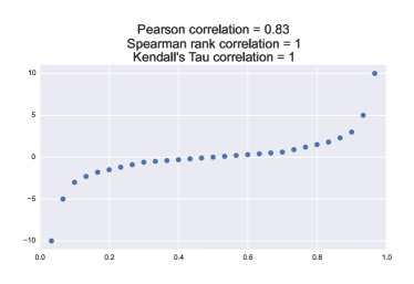
(a) $Y$ is a monotonically increasing function of $X$

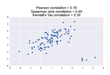
(b) Data with outliers

Figure 1: Comparison of Pearson correlation, Spearman’s rank correlation, and Kendall’s tau correlation on simulated data.

One drawback of SR and KT compared with Pearson correlation is that they require more computational time. The computation of SR and KT requires sorting (finding rank) of the $X$ and $Y$ sequences, which is a very time-consuming step when the sample size $n$ is large. The minimum time complexities for batch algorithms for SR and KT are $O(n\log n)$ [10], whereas the time complexity for batch algorithm of Pearson correlation is $O(n)$.

In practice you sometimes would want to analyze correlation between variables in dynamic environments, where the data are streaming in. These environments include network monitoring, sensor networks, and financial analysis. A good algorithm should make it easy to incorporate new data and process the input sequence in a serial fashion. Such algorithms are called online algorithms in this paper. Online algorithms have interesting applications in various fields [11, 12, 13, 14]. A standard online algorithm exists to compute Pearson correlation by using the idea of sufficient statistics [13]. The time complexity of this algorithm is $O(1)$, and its memory cost is also $O(1)$. However, because Pearson correlation is not robust against outliers, it is not the desirable method for some applications, for example, suppose you collect data from a huge sensor network of a complex system and you want to analyze the correlation in order to detect highly correlated sensor pairs. Outliers in sensor readings might occur because of noise, different temperature conditions, or failures of sensors or communication. Pearson correlation would not be robust enough to handle such an analysis.

This type of analysis demonstrates the need for an online algorithm for nonparametric correlations (such as SR and KT). However, the way the Pearson correlation is computed cannot be directly carried over to SR and KT. It cannot be carried over for SR because new data can change the ranks of all historical observations that were used to compute the correlation. For KT on the other hand, new data need to be compared with all historical data in the computation of the correlation. In order to compute SR and KT with streaming data exactly, it is necessary to keep all previous history in memory, which is impossible because the data streams can be unbounded in length.

This paper proposes an efficient online algorithm for SR and KT. The time complexity of this algorithm is $O(1)$, and its memory cost is also $O(1)$. Although the algorithm only approximately computes SR and KT, this paper shows through extensive simulation studies and real applications that the approximation is good enough for most cases. To the limit of the authors’ knowledge, the algorithm developed in this work is the first online algorithm for nonparametric correlation.

2 Online Algorithms for Nonparametric Correlations

Let $\{(x_{i},y_{i}),i\geq 1\}$ denote the streaming inputs of two time series $x$ and $y$. At time $t$, the Pearson correlation ($r_{P}$), Spearman’s rank correlation ($r_{SR}$), and Kendall’s tau correlation ($r_{KT}$) computed based on all previous observations are defined as:

$$r_{P}\triangleq \cfrac{\sum_{i=1}^{t}(x_{i}-\bar{x})(y_{i}-\bar{y})}{\sqrt{\sum_{i=1}^{t}(x_{i}-\bar{x})^{2}\sum_{i=1}^{t}(y_{i}-\bar{y})^{2}}}$$

$$r_{SR}\triangleq \cfrac{\sum_{i=1}^{t}(u_{i}-\bar{u})(v_{i}-\bar{v})}{\sqrt{\sum_{i=1}^{t}(u_{i}-\bar{u})^{2}\sum_{i=1}^{t}(v_{i}-\bar{v})^{2}}}$$

$$r_{KT}\triangleq \cfrac{P-Q}{\sqrt{(P+Q+T)*(P+Q+U)}}$$

where $u_{i}$ is the rank of $x_{i}$, $v_{i}$ is the rank of $y_{i}$, $P$ is the number of concordant pairs, $Q$ is the number of discordant pairs, $T$ is the number of ties only in $x$, and $U$ is the number of ties only in $y$.

The main idea in designing the online algorithms for nonparametric correlations is to coarsen the bivariate distribution of ($X$,$Y$). The coarsened joint distribution can represented by using a small matrix. Assume that both $X$ and $Y$ are continuous random variables. You provide $m_{1}^{*}$ and $m_{2}^{*}$ distinct cutpoints in ascending order for $X$ and $Y$ respectively, where both $m_{1}^{*}$ and $m_{2}^{*}$ are nonnegative integers. The cutpoints for $X$ are denoted as $(c^{x}_{1}$,…,$c^{x}_{m_{1}^{*}})^{\mbox{\tiny{\sf T}}}$, where $c^{x}_{1}<c^{x}_{2}<\ldots<c^{x}_{m_{1}^{*}}$. Similarly, the cutpoints for $Y$ are represented as $(c^{y}_{1}$,…,$c^{y}_{m_{2}^{*}})^{\mbox{\tiny{\sf T}}}$. Two default cutpoints are added for $X$: $c^{x}_{0}$ and $c^{x}_{m_{1}^{*}+1}$, where $c^{x}_{0}=-\infty$ and $c^{x}_{m_{1}^{*}+1}=\infty$. Cutpoints $\{c^{x}_{i},\,i=0\ldots,m_{1}^{*}+1\}$ discretize $X$ into $m_{1}$ ranges, where $m_{1}=m_{1}^{*}+1$. The same is done for $Y$, and cutpoints $\{c^{y}_{i},\,i=0\ldots,m_{2}^{*}+1\}$ discretize $Y$ into $m_{2}$ ranges, where $m_{2}=m_{2}^{*}+1$. The $m_{1}\times m_{2}$ count matrix $M$ is then constructed, where $M[i,j]$ stores the number of observations that falls into the range $[c^{x}_{i-1},c^{x}_{i})\times[c^{y}_{j-1},c^{y}_{j})$. An example of an $M$ matrix is shown in Figure 2, where three cutpoints are chosen for $X$ and four cutpoints are chosen for $Y$. Using the count matrix $M$ has two advantages: first, instead of entire $(x_{i},y_{i})$ series (which maybe unbounded in length) being stored,the information is stored in a matrix of fixed size. Second, when $(x_{i},y_{i})$ are discretized and stored in $M$, they are naturally sorted, and fast algorithms exist to quickly compute $r_{SR}$ and $r_{KT}$ from $M$. This paper proves that the time complexity of the algorithms is $O(m_{1}m_{2})$ for both Spearman’s rank correlation and Kendall’s tau correlation. Because both $m_{1}$ and $m_{2}$ are fixed integers, the algorithms for both Spearman’s rank correlation and Kendall’s tau have $O(1)$ time complexity and $O(1)$ memory cost. This makes the implementation of these algorithms quite attractive on edge devices, where only limited memory and processing power are available. In practice cutpoints for $X$ and $Y$ need to be chosen. One good choice for cutpoints are the equally spaced quantiles of the random variable. For example, to choose 9 cutpoints for $X$, we can use the sample quantiles of $X$ that correspond to the probabilities $0.1,0.2,\ldots,0.9$.

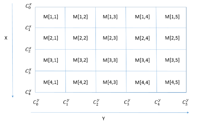
Figure 2: Example of count matrix $M$ with three cutpoints of $x$ and four cutpoints of $y$.

The preceding discussion assumes that both $X$ and $Y$ are continuous. When $X$ and $Y$ are discrete or ordinal, cutpoints can be selected so that each pair of consecutive cutpoints contains only one level of the random variable. When both $X$ and $Y$ are discrete or ordinal no information is lost by using $M$ to approximate the bivariate distribution of ($X$, $Y$), and the algorithm’s result is the exact nonparametric correlation between $X$ and $Y$.

The general online algorithm for SR and KT is given in Algorithm 1. To expedite the computation, not only is matrix $M$ tracked, but also its row sum $n_{\mathrm{row}}=(n_{\mathrm{row}}[1],\ldots,n_{\mathrm{row}}[m_{1}])^{\mbox{\tiny{\sf T}}}$, its column sum $n_{\mathrm{col}}=(n_{\mathrm{col}}[1],\ldots,n_{\mathrm{col}}[m_{2}])^{\mbox{\tiny{\sf T}}}$, and its total sum $n=\sum_{i=1}^{m_{1}}\sum_{j=1}^{m_{2}}M[i,j]$. The algorithm is also designed to compute nonparametric correlation and return the result every $n_{\mathrm{gap}}$ new observations. The $n_{\mathrm{gap}}$ is a user-specified parameter, where $n_{\mathrm{gap}}\geq 1$. When the observation index $t$ mod $n_{\mathrm{gap}}$ is not equal to 0, only $M$, $n_{\mathrm{row}}$, $n_{\mathrm{col}}$, and $n$ need to be updated (Step 3–6), and the nonparametric correlation does not need to be computed (Step 8) in the iteration. When $t$ mod $n_{\mathrm{gap}}$ is equal to 0, it is necessary both to update $M$, $n_{\mathrm{row}}$, $n_{\mathrm{col}}$ and $n$, and to compute the nonparametric correlation. Unlike the step that computes the nonparametric correlation, the updating steps can be done very efficiently with time complexity $O(\max(\log(m_{1}),\log(m_{2})))$.

1 Input: $\{(x_{t},y_{t})\}_{t=1}^{T}$ (streaming observations), $(c^{x}_{1}$,…,$c^{x}_{m_{1}})^{\mbox{\tiny{\sf T}}}$ (cutpoints for $x$), $(c^{y}_{1}$,…,$c^{y}_{m_{2}})^{\mbox{\tiny{\sf T}}}$ (cutpoints for $y$), $n_{\mathrm{gap}}$.

2 for t=1 to $T$ do

3       Reveal the sample $(x_{t},y_{t})$.

4       Compare $x_{t}$ with $(c^{x}_{1}$,…,$c^{x}_{m_{1}})^{\mbox{\tiny{\sf T}}}$ and find the row index $i$ of $M$ that corresponds to the observation via a binary search.

5       Compare $y_{t}$ with $(c^{y}_{1}$,…,$c^{y}_{m_{2}})^{\mbox{\tiny{\sf T}}}$ and find the column index $j$ of $M$ that corresponds to the observation via a binary search.

6       $M[i,j]\leftarrow M[i,j]+1$, $n_{\mathrm{row}}[i]\leftarrow n_{\mathrm{row}}[i]+1$, $n_{\mathrm{col}}[j]\leftarrow n_{\mathrm{col}}[j]+1$, $n\leftarrow n+1$

7       if $t$ mod $n_{\mathrm{gap}}=0$  then

8             Compute the nonparametric correlation based on $M$, $n_{\mathrm{col}}$, $n_{\mathrm{row}}$, $n$, and save the result to $r[t]$.

9      

return $(r[n_{\mathrm{gap}}],r[2n_{\mathrm{gap}}],\ldots)^{\mbox{\tiny{\sf T}}}.$

Algorithm 1 General online algorithm for nonparametric correlation

Step 8 in Algorithm 1 is described in detail for SR and KT respectively in Algorithms 2 and 3, where the nonparametric correlations are quickly computed based on matrix $M$, $n_{\mathrm{row}}$, $n_{\mathrm{col}},$ and $n$. It is easy to verify that the time complexity of both algorithms is $O(m_{1}m_{2})$ in linear proportion to the number of cells in matrix $M$.

1 Input: $M$, $n_{\mathrm{row}}$, $n_{\mathrm{col}}$, $n$, $m_{1}$, and $m_{2}$

2 # iteratively compute the rank that corresponds to each row of $M$

3 $r=0$

4 for k=1 to $m_{1}$ do

5       if $n_{\mathrm{row}}[k]=0$ then

6             $r_{\mathrm{row}}[k]\leftarrow r$

7      else

8             $r_{\mathrm{row}}[k]\leftarrow[(r+1)+(r+n_{\mathrm{row}}[k])]/2$

9             $r\leftarrow r+n_{\mathrm{row}}[k]$

10      

11# iteratively compute the rank that corresponds to each column of $M$.

12 $r=0$.

13 for k=1 to $m_{2}$ do

14       if $n_{\mathrm{col}}[k]=0$ then

15             $r_{\mathrm{col}}[k]\leftarrow r.$

16      else

17             $r_{\mathrm{col}}[k]\leftarrow[(r+1)+(r+n_{\mathrm{col}}[k])]/2$

18             $r\leftarrow r+n_{\mathrm{col}}[k].$

19      

20$r^{*}_{\mathrm{row}}\leftarrow r_{\mathrm{row}}-(n+1)/2$; $r^{*}_{\mathrm{col}}\leftarrow r_{\mathrm{col}}-(n+1)/2.$

21 $r^{*}_{\mathrm{row}}\leftarrow r^{*}_{\mathrm{row}}/\sqrt{\sum_{i=1}^{m_{1}}n_{\mathrm{row}}[i]r^{*}_{\mathrm{row}}[i]^{2}}$; $r^{*}_{\mathrm{col}}\leftarrow r^{*}_{\mathrm{col}}/\sqrt{\sum_{i=1}^{m_{2}}n_{\mathrm{col}}[i]r^{*}_{\mathrm{col}}[i]^{2}}.$

22 $corr\leftarrow(r^{*}_{\mathrm{row}})^{\mbox{\tiny{\sf T}}}Mr^{*}_{\mathrm{col}}.$

return $corr.$

Algorithm 2 Compute Spearman’s rank correlation based on matrix $M$

1 Input: $M$, $n_{\mathrm{row}}$, $n_{\mathrm{col}}$, $n$, $m_{1}$, and $m_{2}$.

2 Initialize $N$ as an $m_{1}$ by $m_{2}$ zero matrix.

3 Compute $P$ (the number of concordant pairs):

4 for i=2 to $m_{1}$ do

5       for j=2 to $m_{2}$ do

6             if j=2 then

7                   $N[i,j]\leftarrow M[i-1,j-1]$

8            else

9                   $N[i,j]\leftarrow N[i,j-1]+M[i-1,j-1]$

10            

11      

12for i=2 to $m_{1}$ do

13       $N[i,:]\leftarrow N[i,:]+N[i-1,:]$

14$P=\sum_{i=1}^{m_{1}}\sum_{j=1}^{m_{2}}M[i,j]*N[i,j]$

15 Compute $T$ (the number of ties only in x): $T=[\sum_{i=1}^{m_{1}}(n_{\mathrm{row}}[i]^{2}-\sum_{j=1}^{m_{2}}M[i,j]^{2})]/2$

16 Compute $U$ (the number of ties only in y): $T=[\sum_{j=1}^{m_{2}}(n_{\mathrm{col}}[j]^{2}-\sum_{i=1}^{m_{1}}M[i,j]^{2})]/2$

17 Compute $B$ (the number of ties in both x and y): $B=\sum_{i=1}^{m_{1}}\sum_{j=1}^{m_{2}}M[i,j]*(M[i,j]-1)/2$

18 Compute $Q$ (the number of discordant pairs): $Q=(n+1)*n/2-P-T-U-B$

19 $corr\leftarrow(P-Q)/\sqrt{(P+Q+T)*(P+Q+U)}$

return $corr.$

Algorithm 3 Compute Kendall’s tau correlation based on matrix $M$

The parameters $(m_{1},m_{2})$ control a tradeoff between the accuracy and efficiency of the online algorithms. The more cutpoints that are chosen for $x$ and $y$ (larger $m_{1}$, $m_{2}$), the more accurate the approximation of the bivariate distribution of $(x,y)$ with $M$ and a more accurate result is generally achieved. However, increasing $m_{1}$ and $m_{2}$ also decreases the speed of the online algorithm. Based on the extensive numerical studies of the next section, a rule-of-thumb choice of $(m_{1},m_{2})$ is $m_{1}=m_{2}=30$ for SR and $m_{1}=m_{2}=100$ for KT.

In practice, the proposed online algorithms for nonparametric correlations usually work well for the following reasons: First, when $(m_{1},m_{2})$ increase to infinity, the result of online algorithms converges to the true value. Second, for a reasonably large $(m_{1},m_{2})$, each cell of matrix $M$ represents only a very local area of the $(X,Y)$ distribution. Positive errors and negative errors can cancel each other out when summed together.

Algorithms  2 and 3 compute SR and KT over all past data. Frequently, you are interested in computing the statistics only over the recent past. Specifically, you might like to compute SR and KT with a sliding window of a fixed size. Algorithm 1 can be easily modified to deal with such cases. The only change that is needed is to add some steps after step 6; in the added steps $M$, is updated by first finding the row index and the column index that correspond to the observation $(x_{t-n_{\mathrm{win}}},y_{t-n_{\mathrm{win}}})$ and then decreasing the corresponding cell of $M$ by 1. Here $n_{\mathrm{win}}$ represents the size of the sliding windows. The details are left to the readers.

3 Simulation Studies

In the following simulation studies, equal numbers of cutpoints are always chosen for both $X$ and $Y$, and all cutpoints are chosen as equally spaced quantiles of a standard normal distribution. We implement the batch and online nonparametric correlation algorithms in python. Users can download the package from https://github.com/wxiao0421/onlineNPCORR.git.

3.1 Simulation Study with Nonparametric Correlations Computed over All Past Observations

This simulation evaluates the online algorithms for SR and KT (computed over all past observations) by comparing them with the corresponding batch algorithms. The $x_{i}$, $i=1,\ldots,T$ are generated from an independently and indentically distributed (iid) normal distribution $N(0,1)$. Let $y_{i}=(z_{i}+\sigma x_{i})/\sqrt{\sigma^{2}+1}$, where $z_{i}$, $i=1,\ldots,T$ are iid $N(0,1)$ random variables, which are independent of $x_{i}$, $i=1,\ldots,T$. It is easy to verify that both $\{x_{i}\}_{i=1}^{T}$ and $\{y_{i}\}_{i=1}^{T}$ are iid $N(0,1)$ with a Pearson correlation coefficient of $\sigma/\sqrt{\sigma^{2}+1}$.

The result for SR is shown in Figure 3. All numbers are averaged over 10 replications. All results in subplots (a) and (b) are based on $n_{\mathrm{gap}}=1$. Subplot (a) compares the run times of the batch algorithm and the online algorithms with different numbers of cutpoints. It is clear that for the online algorithms, increasing the number of cutpoints decreases the speed of the algorithms. Furthermore, as the number of observations ($T$) increases, the differences between the run times for the batch algorithm and the online algorithm also increase dramatically. The SR algorithm with 20 cutpoints (online SR (20)) takes less than 10 seconds to run a $T=10^{5}$ case, whereas the batch algorithm takes more than 1,000 seconds. When $T$ increases to $10^{6}$, the batch algorithm becomes too slow to handle such cases (time complexity $O(T^{2}\log T)$), whereas it is easy to both numerically and theoretically prove that the run time of the online algorithm is proportional to $T$. Subplot (b) compares the L1 error of the estimated Spearman’s rank correlation from the online algorithm with different numbers of cutpoints (computed at $T$). The L1 error does not seem to increase with $T$, and it generally decreases with the number of cutpoints. For all cases, the L1 error is kept below 0.004. Subplot (c) compares the run times of the online algorithm (with 50 cutpoints) for $n_{\mathrm{gap}}=1$ and $100$. The increase in speed is 30-fold for $n_{\mathrm{gap}}=100$ for all $T$. Last, the batch algorithm is implemented very efficiently in C (using the Python Scipy package) whereas the online algorithm is Purely python code. So if the online algorithm is also implemented in C, you would likely see another 10 to 100-fold speed increase for the online algorithm.

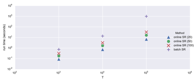
(a) Run times with different numbers of cutpoints ($n_{\mathrm{gap}}=1$)

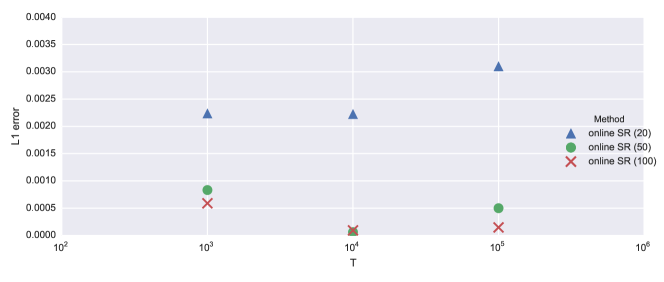
(b) $L_{1}$ errors ($n_{\mathrm{gap}}=1$)

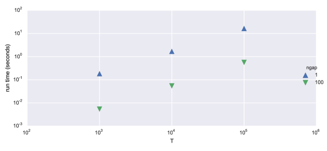
(c) Run times with different $n_{\mathrm{gap}}$ (online SR (50))

Figure 3: Comparison of online algorithm and batch algorithm for Spearman’s rank correlation, where “online SR (K)” represents the online algorithm with 50 cutpoints for both $X$ and $Y$ variables. All cutpoints of $X$ and $Y$ are chosen as equally spaced quantiles of a standard normal distribution.

The result for KT is shown in Figure 4. Subplot (a) compares the run times of the batch algorithm and the online algorithm with different numbers of cutpoints. The observed pattern is similar to that of SR, where the run times increase with the number of cutpoints in the online algorithm. Furthermore, as the number of observations ($T$) increases, the differences between the run times of the batch algorithm and online algorithm also increase dramatically. The KT online algorithm with 100 cutpoints (online KT (100)) takes approximately 10 seconds to run a $T=10^{4}$ case, whereas the batch algorithm takes more than 1,000 seconds. When $T$ increases to $10^{5}$, the batch algorithm becomes too slow to handle such cases, whereas the online algorithm can still finish the computation in a very short period of time. Subplot (b) compares the L1 error of the estimated Kendall’s tau correlation of the online algorithm with different numbers of cutpoints (computed at $T$). The L1 error does not seem to change much with $T$, and it decreases with the number of cutpoints. For all cases where the number of cutpoints is larger than 50, the L1 error is below 0.01. Subplot (c) compares the run times of the online algorithm under $n_{\mathrm{gap}}=1$ and $100$ (with 50 cutpoints). You see increases of approximately 60 to 70 times for $n_{\mathrm{gap}}=100$ and all $T$.

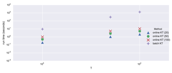
(a) Run times with different numbers of cutpoints ($n_{\mathrm{gap}}=1$)

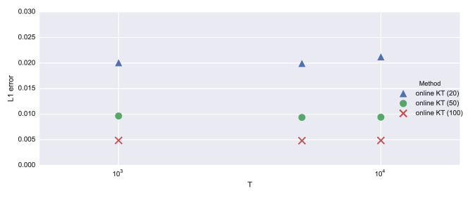
(b) $L_{1}$ errors ($n_{\mathrm{gap}}=1$)

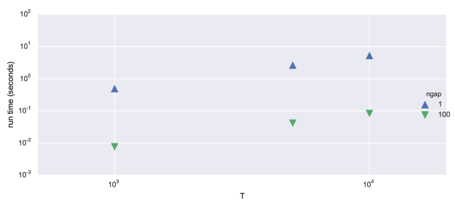
(c) Run times with different $n_{\mathrm{gap}}$ (online KT (50))

Figure 4: Comparison of online algorithm and batch algorithm for Kendall’s tau correlation, where “online KT (K)” represents online algorithm with 50 cutpoints for both $X$ and $Y$ variables. All cutpoints of $X$ and $Y$ are chosen as equally spaced quantiles of a standard normal distribution.

3.2 Simulation Study with Nonparametric Correlations Computed Based on Sliding Windows

This simulation study compares the batch and online algorithms for SR and KT based on sliding windows. Generate $x_{i}$, $i=1,\ldots,T$ from an iid normal distribution $N(0,1)$. Let $y_{i}=(z_{i}+\sigma(i)x_{i})/\sqrt{\sigma(i)^{2}+1}$, where $z_{i}$, $i=1,\ldots,T$ are iid $N(0,1)$ random variables, which are independent with $x_{i}$, $i=1,\ldots,T$. Then $T=100,000$ and $n_{\mathrm{win}}=10,000$ for SR, and $T=10,000$ and $n_{\mathrm{win}}=1,000$ for KT. We choose $\sigma(i)=5[(i-m)/m]^{2}$, where $m=50,000$ for SR and $m=5,000$ for KT.

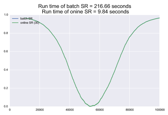
(a) Spearman’s rank correlation ($n_{\mathrm{gap}}=1$)

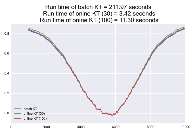
(b) Kendall’s tau correlation ($n_{\mathrm{gap}}=1$)

Figure 5: Comparison of online and batch algorithms for Spearman’s rank correlation and Kendall’s tau correlation based on sliding windows where “online SR (K)” and “online KT (K)” represents the online algorithm for SR and KT with 50 cutpoints (for both $X$ and $Y$ variables). All cutpoints of $X$ and $Y$ are chosen as equally spaced quantiles of standard normal distribution.

The results are shown in Figure 5. The SR online algorithm generates a very accurate estimate of Spearman’s rank correlation even when the number of cutpoints is small ($m_{1}=m_{2}=30$). The KT online algorithm seems to generate a very accurate estimate of the Kendall’s tau correlation when the absolute value of the correlation is small, but it seems to generate a more biased estimate when the absolute value of the correlation is large. This is because when $x$, $y$ are highly correlated, the $(x_{i},y_{i})$ pairs are likely to be concentrated on the diagonal of matrix $M$. This concentration leads to a poor approximation of the bivariate distribution of $(x,y)$ with matrix $M$, which leads to biased estimates of Kendall’s tau correlation. For the KT online algorithm we suggest keeping the number of cutpoints above 100 in order to achieve a more accurate result.

4 Application to Sensor Data Generated in Industrial plant

This section uses the proposed online algorithms to compute nonparametric correlations based on sensor data that were generated in industrial plant from 2015 Prognostics and Health Management Society Competition [15]. The data contains sensor readings of 50 plants. For each plant, it provides sensor readings of four standard sensors S1-S4, and four control sensors R1-R4. We use the sensor readings of the first component in the first plant to do our experiment, where we compute nonparametric correlations based on sliding windows with window size 35,040 (corresponds to a one-year window).

First, we compute the nonparametric correlation between $R_{1}$ and $S_{1}$. $R_{1}$ contains 10 unique values and we choose 9 cutpoints so that each unique value has its own cell in matrix $M$. $S_{1}$ has 121 unique values, and we experiment on two methods to choose cutpoints for $S_{1}$. In the first method, we choose 120 cutpoints for $S_{1}$ so that each unique value of $S_{1}$ has its own cell in matrix $M$. In the second method, the cutpoints are chosen by first computing sample quantiles of $S_{1}$ at probabilities $0.05,0.10,\ldots,0.95$, and keeping only the unique values. This leads to choosing 19 cutpoints for $S_{1}$. The result is shown in Figure 6. We refer the result of the online algorithm with 19 cutpoints for $S_{1}$ as online SR (approximate) and online KT (approximate), respectively. Because the returned nonparametric correlations will only approximately equal the true values. We see a 20-50 fold speed up for SR and 5-20 fold speed up for KT.

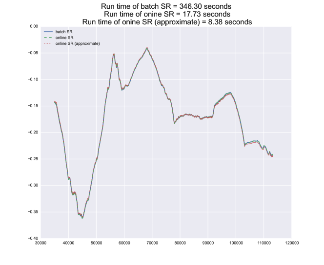
(a) Spearman’s rank correlation

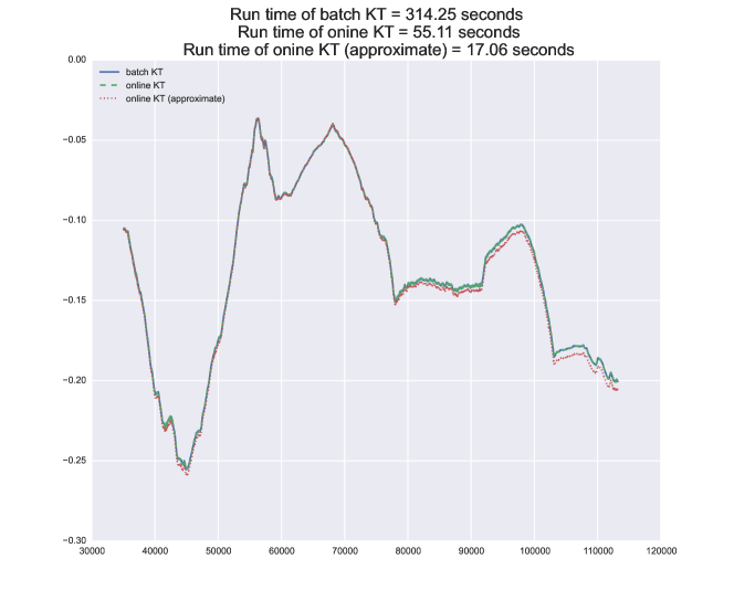
(b) Kendall’s tau correlation

Figure 6: Computation of nonparametric correlations between $R_{1}$ and $R_{1}$ with fixed size sliding windows.

Then, we compute the nonparametric correlation between $R_{3}$ and $S_{3}$. We choose 7 cutpoints for $R_{3}$ and 11 cutpoints for $S3$ so that each unique value of $R_{3}$ and $S_{3}$ has its own cell in matrix $M$. The result is shown in Figure 7. The online algorithm returns the same result as that of batch algorithm with a 20-40 fold speed up.

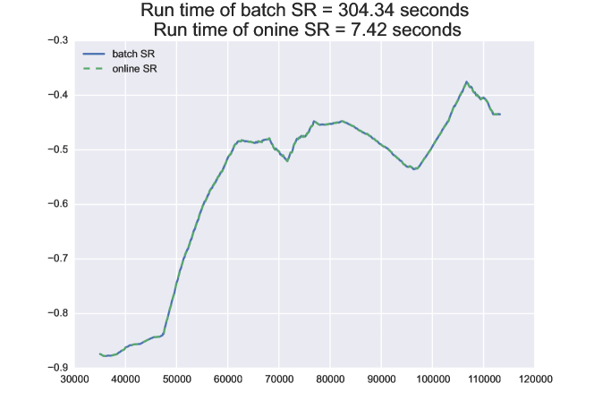
(a) Spearman’s rank correlation

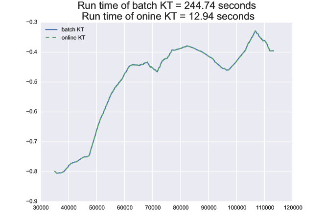
(b) Kendall’s tau correlation

Figure 7: Computation of nonparametric correlations between $R_{2}$ and $R_{3}$ with fixed size sliding windows.

5 Conclusion

This paper proposes a novel online algorithm for the computation of Spearman’s rank correlation and Kendall’s tau correlation. The algorithm has time complexity $O(1)$ and memory cost $O(1)$, and it is quite suitable for edge devices, where only limited memory and processing power are available. By changing the number of cutpoints specified in the algorithm, users can seek a balance between speed and accuracy. The new online algorithm is very fast and can easily compute the correlations 10 to 1,000 times faster than the corresponding batch algorithm (the number varies over the settings of the problem). The online algorithm can compute nonparametric correlations based either on all past observations or on fixed-size sliding windows.

References

- [1] P. J. Huber, Robust Statistics. Springer, 2011.
- [2] P. J. Rousseeuw and A. M. Leroy, Robust Regression and Outlier Detection, vol. 589. John wiley & sons, 2005.
- [3] A. Zaman, P. J. Rousseeuw, and M. Orhan, “Econometric applications of high-breakdown robust regression techniques,” Economics Letters, vol. 71, no. 1, pp. 1–8, 2001.
- [4] W. Xiao, H. H. Zhang, and W. Lu, “Robust regression for optimal individualized treatment rules,” arXiv preprint arXiv:1604.03648, 2016.
- [5] O. Grothe et al., “Estimating correlation and covariance matrices by weighting of market similarity,” tech. rep., arXiv. org, 2010.
- [6] E. S. Fritz, “Total diet comparison in fishes by spearman rank correlation coefficients,” Copeia, pp. 210–214, 1974.
- [7] T. Franceschini, J.-D. Bontemps, V. Perez, and J.-M. Leban, “Divergence in latewood density response of norway spruce to temperature is not resolved by enlarged sets of climatic predictors and their non-linearities,” Agricultural and Forest Meteorology, vol. 180, pp. 132–141, 2013.
- [8] C. Croux and C. Dehon, “Influence functions of the spearman and kendall correlation measures,” Statistical methods & applications, vol. 19, no. 4, pp. 497–515, 2010.
- [9] S. J. Devlin, R. Gnanadesikan, and J. R. Kettenring, “Robust estimation and outlier detection with correlation coefficients,” Biometrika, vol. 62, no. 3, pp. 531–545, 1975.
- [10] W. R. Knight, “A computer method for calculating kendall’s tau with ungrouped data,” Journal of the American Statistical Association, vol. 61, no. 314, pp. 436–439, 1966.
- [11] K. Crammer and Y. Singer, “Ultraconservative online algorithms for multiclass problems,” Journal of Machine Learning Research, vol. 3, no. Jan, pp. 951–991, 2003.
- [12] N. C. Oza, “Online bagging and boosting,” in Systems, Man and Cybernetics, 2005 IEEE international conference on, vol. 3, pp. 2340–2345, IEEE, 2005.
- [13] J. Gama, Knowledge Discovery from Data Streams. CRC Press, 2010.
- [14] W. Xiao, X. Huang, J. Silva, S. Emrani, and A. Chaudhuri, “Online robust principal component analysis with change point detection,” arXiv preprint arXiv:1702.05698, 2017.
- [15] J. Rosca, Z. Song, N. Willard, and N. Eklund PHM15 Challenge Competition and Data Set: Fault Prognostics, NASA Ames Prognostics Data Repository (http://ti.arc.nasa.gov/project/prognostic-data-repository), NASA Ames Research Center, Moffett Field, CA, 2015.