Atomic Norm Based Localization of Far-Field and Near-Field Signals with Generalized Symmetric Arrays
Abstract
Most localization methods for mixed far-field (FF) and near-field (NF) sources are based on uniform linear array (ULA) rather than sparse linear array (SLA). In this paper, we propose a localization method for mixed FF and NF sources based on the generalized symmetric linear arrays, which include ULAs, Cantor array, Fractal array and many other SLAs. Our method consists of two steps. In the first step, the high-order statistics of the array output is exploited to increase the degree of freedom. Then the direction-of-arrivals (DOAs) of the FF and NF sources are jointly estimated by using the recently proposed atomic norm minimization (ANM), which belongs to the gridless super-resolution method since the discretization of the parameter space is not required. In the second step, the ranges are given by MUSIC-like one-dimensional searching. Simulations results are provided to demonstrate the advantages of our method.
Index Terms— Source localization, far-field, near-field, generalized symmetric arrays, atomic norm minimization.
1 Introduction
Source localization is a fundamental problem in array signal processing and has received considerable attention. Based on the far-field (FF) source assumption where the impinged signals are assumed to be plane-wave, numerous methods have been proposed for FF source localization, i.e., direction-of-arrival (DOA) estimation [1, 2, 3, 4, 5][6]. However, when the sources are close to the array and lie in the near-field (NF) region (i.e., the Fresnel region), the impinged signals are spherical wave rather than plane-wave. In this case, the steering vectors are characterized by two independent parameters: DOA and range. Hence, the DOA estimation methods for FF source localization can not be applied to the NF source localization. In order to deal with this problem, the nonlinear time delay of the spherical wavefront model is approximated into a quadratic wavefront model by using the second-order Taylor expansion. Based on this approximation, a large number of NF source localization methods have been proposed. For instance, He et al. have proposed an oblique projection based MUSIC (OPMUSIC) algorithm for mixed FF and NF sources localization [7]. An efficient subspace-based localization method without eigendecomposition has been proposed in [8]. However, the maximum number of resolvable sources of these methods are limited to half of the number of sensors. Liang et al. have proposed a cumulant based algorithm called two-stage MUSIC (TSMUSIC) by using the high-order statistics (HOS) of the array output [9]. By using the HOS and compressed sensing theory, a sparse method has been presented for mixed sources localization [10]. However, sparse method requires to discretize the angle space hence its performance is limited by the so called ”basis mismatch” effect. Note that, all the aforementioned methods are proposed based on the uniform linear array (ULA) and most of them can not be extended to the sparse linear array (SLA). As a result, the maximum number of resolvable sources of these methods can not exceed the number of sensors.
Recently, the SLA has been studied in FF DOA estimation by exploiting the coarray of the physical array to increase the array aperture [11, 12, 13, 14]. Due to the extended array aperture, the resolution and the maximum number of resolvable sources can be greatly improved. Nevertheless, the classical SLAs, e.g., coprime array, nested array can not be directly employed for NF source localization since most of the NF source localization methods require symmetric array structure. By using the special geometry of the nested array (i.e., two subarrays without overlapping), several symmetric nested arrays have been proposed [15, 16]. However, these literatures focus on constructing specific SLA to extend the array aperture. A unified algorithm for generalized symmetric SLA in NF source localization area is still missing. Furthermore, all these methods choose MUSIC for DOA estimation which suffers from basis mismatch effect.
In this paper, we propose a unified localization method for mixed FF and NF sources which can be applied to any sparse/uniform symmetric redundancy array. The high-order cumulants of the array output are exploited to increase the degrees-of-freedom (DoFs). The atomic norm is employed to eliminate the basis mismatch effect in DOA estimation and able to provide super-resolution. Moreover, the proposed method does not require the prior knowledge of the noise power as well as the number of sources or FF/NF sources.
2 Signal Model
We first give the definition of the generalized symmetric linear array that will be used throughout of this paper. Let . The indices of the array sensors are denoted as where are non-negative unequal integers and sorted ascendingly with and . Due to the symmetric property of the array, we have . Let denote the cardinality of , it is easy to see that . If , represents a symmetric ULA while if , represents a symmetric SLA. It should be noted that ULA can be regarded as a special case of SLA. As a result, only the SLA case is considered in the rest of this paper. We then provide the definition of coarray below.
Definition 1
The coarray of a physical array is defined as, . is called a redundancy array if (a.k.a. hole-free coarray). Otherwise, is called a non-redundancy array.
It is shown that the maximum number of detectable sources using the array is determined by its coarray rather than the number of physical sensors [17]. In fact, a redundancy array is able to detect up to sources, which is greater than its number of sensors if . To better understand our array, we here provide a simple example.
Example 1
A symmetric SLA with has the coarray which is hole-free. By using proper algorithms, the array can detect up to sources, which is greater than the number of sensors.
It should be pointed out that the aforementioned symmetric SLAs with hole-free coarray not only include the array in Example 1, but also contain the recently proposed cantor array [18] and fractal array [19].111Note that the factal array is able to extend any known symmetric redundancy array to a much larger one. . In fact, the proposed method can be applied to any symmetric redundancy array. To avoid the angle ambiguity, the minimum sensor spacing should satisfy where is the wavelength.
We then assume narrowband uncorrelated mixed FF and NF sources impinge onto the array and the -th source is characterized by a parameter pair . The array output is given by,
| (1) |
where is the array output, is the signal waveform, denotes the additive white Gaussian noise with zero mean and denotes the manifold matrix of the array, in which is the steering vector of the -th signal with
| (2) |
| (3) |
Note that we unify the steering vectors of the FF and NF sources as since the steering vector of the FF source can be represented as .
3 The Proposed Method
3.1 DOA Estimation of FF and NF Sources
Similar to TSMUSIC, the fourth-order cumulants are utilized to construct a Hermitian matrix without the range parameter for DOA estimation. Specifically, we define the fourth-order cumulant as
| (4) |
where , , and is the fourth-order cumulant of .222Since many practical signals such as sinusoidal signal, amplitude shift keying (ASK) signal and phase shift keying (PSK) signal are sub-Gaussian process, we assume is zero-mean stationary random processes with negative kurtosis, i.e., . can be compactly written as the following Hermitian matrix,
| (5) |
where contains the fourth-order cumulants of the signals, and . It can be seen from (5) that, the range parameter is removed from . Hence matrix can be regarded as the covariance matrix of a virtual array output with manifold matrix which is positive semidefinite (PSD). Although we can apply the subspace based methods such as MUSIC to to estimate the DOAs, directly using MUSIC for DOA estimation can not utilize the coarray property to increase the DoFs. Below we use the atomic norm theory which can fully utilize the coarray to estimate the DOAs.
First, denote as the steering vector of the coarray and as a selecting matrix such that the -th row of contains all s but a single at the -th position. It is clear that and
| (6) |
| (7) |
where denotes the covariance matrix of the coarray output. It can be seen that compared to , has a much larger dimensionality which can be used to increase the DoF. To do this, let’s first rewrite as,
| (8) |
And then define an atom set
| (9) |
Based on the atomic norm theory, the atomic norm of can be defined as
| (10) |
Although (10) provides a proper decomposition of by using the atoms in with respect to the DOAs, it is still unknown how to compute the atomic norm from the definition. To solve this problem, the atomic norm can be transformed to a semidefinite programming (SDP). Formally, we have,
Theorem 1 ([20])
The atomic norm defined in (10) equals the optimal value of the following SDP,
| (11) |
where denotes a Toeplitz matrix with being its first row.
It is shown that the DOAs are encoded in whose -th element can be given as [21]
| (12) |
Hence the DOAs can be retrieved from the Vandermonde decomposition of [22]. Consequently, we propose the following atomic norm minimization (ANM) problem to retrieve ,333The term is omitted for brevity.
| (13) |
In practice, since we can only observe the sample cumulant matrix of the sparse array output rather than the exact one , the DOAs can be retrieved based on the following ANM problem,
| (14) |
where is an upper bound of the noise energy.
Solving the problem (14) by using CVX gives the estimation of . Then the DOAs can be retrieved by using Vandermonde decomposition or the subspace methods such as root-MUSIC.
Remark 1
By exploiting the coarray property of the redundancy array, our method is able to estimate more sources than sensors in terms of DOA estimation. In particular, the maximum number of detectable sources is , which is greater than the number of sensors if .
3.2 Range Estimation of the NF Sources
In the previous part, we constructed a fourth-order cumulant matrix for DOA estimation based on the special structure of the array. In this part, however, it is unable to construct a fourth-order cumulant matrix for range estimation since the array is sparse. Hence, we utilize the covariance matrix of the array output and apply MUSIC-like algorithm to retrieve the ranges. In particular, we first construct the sample covariance matrix and then apply the eigen-decomposition to to obtain the matrix containing eigenvectors of with respect to the minimum eigenvalues. With the estimated DOAs , the range of the -th signal can be obtained by solving the following problem,
| (15) |
which can be solved by 1-D searching. Note that the FF source is a special NF source with , we choose the range searching area as , where is selected to be larger than with being the array aperture. If the estimated range is located in the Fresnel region , the corresponding source is classified as the NF source. On the other hand, if the estimated range is larger than , the source belongs to the FF source and we let . Note that the DOAs and ranges are automatically paired by using (15).
4 Simulation Results
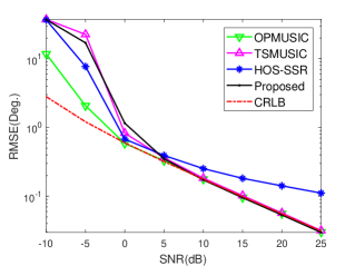
In this section, we evaluate the performance of our proposed method with comparison to OPMUSIC [7], TSMUSIC [9], high-order statistics based sparse signal representation method (HOS-SSR) [10] and the Crammer-Rao lower bound (CRLB) [23].444To reduce complexity, iterative grid refinement procedure is employed in HOS-SSR. The number of sources is assumed to be known for OPMUSIC, TSMUSIC and HOS-SSR but unknown for our method. Meanwhile, OPMUSIC requires the prior knowledge of the number of FF sources.
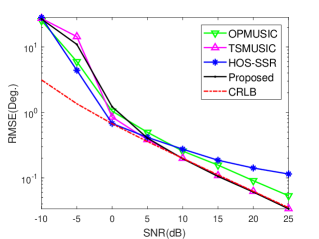
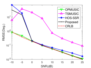
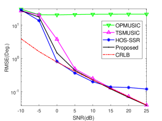
We first consider a -element ULA (i.e., ) with the sensor spacing and assume two narrowband equal-power source signals consisting one FF source from and one NF source from impinge onto the ULA. We set the number of snapshots and evaluate these methods by comparing their RMSEs of the estimates with the SNR varying from dB to dB and show the results in Fig. 1. It can be observed from Fig. 1(a) that our proposed method, OPMUSIC and TSMUSIC are able to approach and coincide with CRLB curve as the SNR grows. HOS-SSR deviates gradually from CRLB because of the model mismatch between the -norm and -norm minimization models. In Fig. 1(b), our method and TSMUSIC can also show satisfying performance whereas OPMUSIC shows worse accuracy since it only utilizes partial information of the covariance matrix of the array output to estimate the DOAs of the NF sources. In Fig. 1(c), we can see that TSMUSIC cannot provide good performance and there exists a large gap between the curves of TSMUSIC and CRLB. In contrast, OPMUSIC and our method can coincide with the CRLB and OPMUSIC performs better in low SNR region. HOS-SSR deviates from the CRLB in range estimation as well.
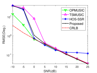
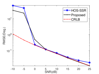
In the second experiment, we replace the ULA with a -element symmetric SLA with and other settings are the same as Fig. 1. From the RMSEs comparison displayed in Fig. 2 we can see that these four methods show similar performance as in the ULA case in DOA estimation of FF source. While for NF source localization, OPMUSIC requires spatial smoothing hence we can observe that it fails in Fig. 2(b). For range estimation, TSMUSIC requires the uniform array structure and thus fails in the SLA case. Therefore, we omit the curves of OPMUSIC and TSMUSIC in Fig. 2(c) from which it can be seen that our proposed method can still approach the CRLB while HOS-SSR deviates from the CRLB as the SNR grows. In summary, our method performs better than other compared methods in DOA and range estimation in both ULA and SLA cases.
5 Conclusions
In this paper, we proposed a mixed source localization based on ANM with symmetric redundancy linear arrays, including ULA, Cantor array, Fractal array and any symmetric redundancy SLAs. The proposed method does not require discretization of the angle space as well as any prior knowledge on the number of sources while still provides super-resolution in DOA and range estimation as compared to subspace and sparse methods in various scenarios.
References
- [1] Ralph Schmidt, “Multiple emitter location and signal parameter estimation,” IEEE Transactions on Antennas and Propagation, vol. 34, no. 3, pp. 276–280, 1986.
- [2] Richard Roy and Thomas Kailath, “ESPRIT-estimation of signal parameters via rotational invariance techniques,” IEEE Transactions on Acoustics, Speech and Signal Processing, vol. 37, no. 7, pp. 984–995, 1989.
- [3] D. Malioutov, M. Çetin, and A. S Willsky, “A sparse signal reconstruction perspective for source localization with sensor arrays,” IEEE Transactions on Signal Processing, vol. 53, no. 8, pp. 3010–3022, 2005.
- [4] C. Zhou, Y. Gu, S. He, and Z. Shi, “A robust and efficient algorithm for coprime array adaptive beamforming,” IEEE Transactions on Vehicular Technology, vol. 67, no. 2, pp. 1099–1112, Feb 2018.
- [5] X. Wu, W. Zhu, and J. Yan, “A high-resolution DOA estimation method with a family of nonconvex penalties,” IEEE Transactions on Vehicular Technology, vol. 67, no. 6, pp. 4925–4938, June 2018.
- [6] Z. Shi, C. Zhou, Y. Gu, N. A. Goodman, and F. Qu, “Source estimation using coprime array: A sparse reconstruction perspective,” IEEE Sensors Journal, vol. 17, no. 3, pp. 755–765, Feb 2017.
- [7] J. He, M. N. S. Swamy, and M. O. Ahmad, “Efficient application of MUSIC algorithm under the coexistence of far-field and near-field sources,” IEEE Transactions on Signal Processing, vol. 60, no. 4, pp. 2066–2070, April 2012.
- [8] W. Zuo, J. Xin, N. Zheng, and A. Sano, “Subspace-based localization of far-field and near-field signals without eigendecomposition,” IEEE Transactions on Signal Processing, vol. 66, no. 17, pp. 4461–4476, Sep. 2018.
- [9] J. Liang and D. Liu, “Passive localization of mixed near-field and far-field sources using two-stage MUSIC algorithm,” IEEE Transactions on Signal Processing, vol. 58, no. 1, pp. 108–120, Jan 2010.
- [10] B. Wang, J. Liu, and X. Sun, “Mixed sources localization based on sparse signal reconstruction,” IEEE Signal Processing Letters, vol. 19, no. 8, pp. 487–490, Aug 2012.
- [11] P. P. Vaidyanathan and P. Pal, “Sparse sensing with co-prime samplers and arrays,” IEEE Transactions on Signal Processing, vol. 59, no. 2, pp. 573–586, Feb 2011.
- [12] P. Pal and P. P. Vaidyanathan, “Nested arrays: A novel approach to array processing with enhanced degrees of freedom,” IEEE Transactions on Signal Processing, vol. 58, no. 8, pp. 4167–4181, Aug 2010.
- [13] C. Zhou, Z. Shi, Y. Gu, and X. Shen, “DECOM: DOA estimation with combined music for coprime array,” in 2013 International Conference on Wireless Communications and Signal Processing, Oct 2013, pp. 1–5.
- [14] C. Zhou, Y. Gu, Y. D. Zhang, Z. Shi, T. Jin, and X. Wu, “Compressive sensing based coprime array direction-of-arrival estimation,” IET Communications, vol. 11, no. 11, pp. 1719–1724, Aug 2017.
- [15] B. Wang, Y. Zhao, and J. Liu, “Mixed-order MUSIC algorithm for localization of far-field and near-field sources,” IEEE Signal Processing Letters, vol. 20, no. 4, pp. 311–314, April 2013.
- [16] Shuang Li and Dongfeng Xie, “Compressed symmetric nested arrays and their application for direction-of-arrival estimation of near-field sources,” Sensors, vol. 16, no. 11, 2016.
- [17] C. Zhou, Y. Gu, Z. Shi, and Y. D. Zhang, “Off-grid direction-of-arrival estimation using coprime array interpolation,” IEEE Signal Processing Letters, vol. 25, no. 11, pp. 1710–1714, Nov 2018.
- [18] C. Liu and P. P. Vaidyanathan, “Maximally economic sparse arrays and cantor arrays,” in 2017 IEEE 7th International Workshop on Computational Advances in Multi-Sensor Adaptive Processing (CAMSAP), Dec 2017, pp. 1–5.
- [19] R. Cohen and Y. C. Eldar, “Sparse fractal array design with increased degrees of freedom,” in ICASSP 2019 - 2019 IEEE International Conference on Acoustics, Speech and Signal Processing (ICASSP), May 2019, pp. 4195–4199.
- [20] C. Zhou, Y. Gu, X. Fan, Z. Shi, G. Mao, and Y. D. Zhang, “Direction-of-arrival estimation for coprime array via virtual array interpolation,” IEEE Transactions on Signal Processing, vol. 66, no. 22, pp. 5956–5971, Nov 2018.
- [21] Gongguo Tang, B.N. Bhaskar, P. Shah, and B. Recht, “Compressed sensing off the grid,” IEEE Transactions on Information Theory, vol. 59, no. 11, pp. 7465–7490, Nov 2013.
- [22] Z. Yang and L. Xie, “On gridless sparse methods for line spectral estimation from complete and incomplete data,” IEEE Transactions on Signal Processing, vol. 63, no. 12, pp. 3139–3153, June 2015.
- [23] E. Grosicki, K. Abed-Meraim, and Yingbo Hua, “A weighted linear prediction method for near-field source localization,” IEEE Transactions on Signal Processing, vol. 53, no. 10, pp. 3651–3660, Oct 2005.