An Empirical Fitting Method to Type Ia Supernova Light Curves. III. A Three-Parameter Relationship: Peak Magnitude, Rise Time, and Photospheric Velocity

Abstract

We examine the relationship between three parameters of Type Ia supernovae (SNe Ia): peak magnitude, rise time, and photospheric velocity at the time of peak brightness. The peak magnitude is corrected for extinction using an estimate determined from MLCS2k2 fitting. The rise time is measured from the well-observed $B$-band light curve with the first detection at least 1 mag fainter than the peak magnitude, and the photospheric velocity is measured from the strong absorption feature of Si II $\lambda$6355 at the time of peak brightness. We model the relationship among these three parameters using an expanding fireball with two assumptions: (a) the optical emission is approximately that of a blackbody, and (b) the photospheric temperatures of all SNe Ia are the same at the time of peak brightness. We compare the precision of the distance residuals inferred using this physically motivated model against those from the empirical Phillips relation and the MLCS2k2 method for 47 low-redshift SNe Ia ($0.005<z<0.04$) and find comparable scatter. However, SNe Ia in our sample with higher velocities are inferred to be intrinsically fainter. Eliminating the high-velocity SNe and applying a more stringent extinction cut to obtain a “low-$v$ golden sample” of 22 SNe, we obtain significantly reduced scatter of $0.108\pm 0.018$ mag in the new relation, better than those of the Phillips relation and the MLCS2k2 method. For 250 km s^-1 of residual peculiar motions, we find 68% and 95% upper limits on the intrinsic scatter of 0.07 and 0.10 mag, respectively.

1. Introduction

The correlation between the light-curve decline rate and the peak luminosity of Type Ia supernovae (SNe Ia), known as the “Phillips relation” (Phillips 1993; Phillips et al. 1999), allows SNe Ia to be used as standardizable candles with many important applications, including measurements of the expansion history that reveal the acceleration of the Universe (Riess et al. 1998; Perlmutter et al. 1999). In the past decade, various efforts have improved the distance estimation, with different parameters adopted to reduce the scatter — for example, with light curves through different filters (Riess et al. 1996; Wang et al. 2003, 2005; Tripp 1998; Guy et al. 2005, 2007; Jha et al. 2007), information about the host galaxies (e.g., Kelly et al. 2010, 2015; Sullivan et al. 2010; Lampeitl et al. 2010; Childress et al. 2013; Rigault et al. 2013, 2015), spectroscopic features (e.g., Wang et al. 2009; Foley & Kasen 2011; Blondin et al. 2011; Fakhouri et al. 2015), and information about color (Wang et al. 2003; Conley et al. 2006) and color-stretch (Burns et al. 2014). Typically, these methods are able to determine the luminosity of individual SNe Ia with an accuracy of 0.14–0.20 mag, or potentially even as low as 0.07 mag (Wang et al. 2009; Foley & Kasen 2011; Rigault et al. 2013, 2015; Kelly et al. 2015; Fakhouri et al. 2015).

In this paper, we introduce a new three-parameter relationship between the peak magnitude, the rise time, and the photospheric velocity at the time of peak brightness, and we apply this to a low-redshift SN Ia sample. This relation may indicate a new direction for further improving the cosmological utility of SNe Ia.

2. Motivation

Assuming that the SN Ia luminosity scales with the surface area of the expanding fireball (which is thought to be approximately a blackbody at early times), and given that optical wavelengths are on the Rayleigh-Jeans tail of the nearly thermal spectrum, the SN Ia luminosity increases quadratically with photospheric radius (see Riess et al. 1999):

$$L\propto R^{2}T\propto[v(t-t_{0})]^{2}T,$$ (1)

where $L$ is the SN luminosity, $R$ is the photospheric radius, $T$ is the fireball temperature, $v$ is the photospheric expansion velocity, $t_{0}$ is the time of first light, and $t-t_{0}$ is the time after first light. Zheng & Filippenko (2017) have shown that, with some further assumptions and replacing a constant photospheric velocity $v$ with a broken-power-law function, the resulting function (Equation 7 of Zheng & Filippenko 2017) can well fit SN Ia light curves. A good application of the fitting method is for estimating the first-light time and the rise time of SNe Ia, as shown by Zheng et al. (2017), where we use the light curve measured about a week to 10 days after the first-light time for a sample of 56 SNe Ia.

Setting the time in Equation 1 to $t_{p}$, the time at peak brightness, one has

$$L_{p}\propto[(v_{p})(t_{p}-t_{0})]^{2}T_{p}.$$ (2)

In addition, one can define $t_{p}-t_{0}$ as the rise time $t_{r}$ (namely, the time since first light until the time of peak brightness in different filters), giving

$$L_{p}\propto(v_{p}t_{r})^{2}T_{p}.$$ (3)

Assuming that the temperature at the time of peak brightness is constant among different SNe Ia, this becomes

$$L_{p}\propto(v_{p}t_{r})^{2},$$ (4)

giving a clear relationship between the peak luminosity ($L_{p}$), the photospheric velocity at the time of peak brightness ($v_{p}$), and the rise time ($t_{r}$). Taking the logarithm of both sides and transforming units into the magnitude system leads to

$$M_{p}=-2.5\,{\rm log}[(v_{p}t_{r})^{2}]+C,$$ (5)

where $M_{p}$ is the absolute magnitude at peak brightness and $C$ is a constant. Equation 5 suggests that the peak magnitude of SNe Ia is directly related to the photospheric velocity at peak brightness ($v_{p}$) and the rise time ($t_{r}$). This is the new relation we are presenting and discussing here. For purposes of convenience, we assign the label $M_{v^{2}t^{2}}$ to represent $-2.5\,{\rm log}[(v_{p}t_{r})^{2}]+C$.

Note that in the above Equation 1, we have assumed optical wavelengths are on the Rayleigh-Jeans tail of the nearly thermal spectrum, but the $B$ broadband filter, which is the band we adopted for the following analysis, has a central wavelength that is too blue to fall on the Rayleigh-Jeans tail for the temperatures of SNe Ia near maximum light; thus, the absolute SN Ia $B$-band magnitudes we measure should have a more complex temperature dependence than the relationship indicates. We have further assumed that the temperature at the time of peak brightness is the same for all SNe Ia, which is not true since various SNe Ia actually exhibit different temperatures (e.g., Nugent et al. 1995). More specifically, subluminous SNe Ia like SN 1991bg (e.g., Filippenko et al. 1992) tend to have a lower temperature near peak brightness (see also Branch et al. 2006), while overluminous SNe Ia like SN 1991T tend to have a higher temperature. Our assumptions are adopted to motivate the parameterization in Equation 5; the scatter caused by differing temperatures will be included in the final dispersion. See Section 4.3 for more discussion of the constant-temperature assumption.

Compared to another well-known correlation among SNe Ia — the Phillips relation, which shows that the peak magnitude is correlated with ${\Delta}m_{15}(B)$, the magnitude drop by 15 days after peak time — there are three major differences. First, the new relation (Equation 5) contains three parameters instead of two parameters as in the Phillips relation; however, similar to ${\Delta}m_{15}(B)$, the other two parameters in Equation 5 are relatively easy to infer. Second, Equation 5 focuses on the rising part of the light curves while the Phillips relation involves the declining part. Third, the new relation has a more straightforward physical explanation (as given in the approximate derivation of Equation 5) compared to the Phillips relation.

In the following section, we will test the new relation by using a sample of SNe Ia having measurements of all three parameters. For comparison purposes, we will also investigate the relation without considering photospheric velocities, namely

$$M_{p}=-2.5\,{\rm log}[(t_{r})^{2}]+C,$$ (6)

which is equivalent to assuming that the photospheric velocity is the same for all SNe Ia at the time of peak brightness. We assign the label $M_{t^{2}}$ to represent $-2.5\,{\rm log}[(t_{r})^{2}]+C$. In the following analysis, the constant $C$ is assigned a value 0 for simplicity; we are interested in relative (rather than absolute) trends.

3. Data Analysis

Zheng et al. (2017) estimated the rise time of 56 SNe Ia selected from the well-observed Lick Observatory Supernova Search (LOSS; Filippenko et al. 2001; Leaman et al. 2011) sample (Ganeshalingam et al. 2010), the third Center for Astrophysics sample (CfA3; Hicken et al. 2009a), and the Carnegie Supernova Project sample (CSP; Contreras et al. 2010). While the details are described by Zheng et al. (2017), here we briefly summarize the rise-time estimation. The rise time is measured from the well-observed $B$-band light curve with the first detection being at least 1 mag fainter than the peak magnitude, in order to measure the first-light time reliably. The $B$ light curve was fit with a variant broken-power-law function to estimate the first-light time along with the time of peak brightness to calculate the rise time. The uncertainty in the rise time is dominated by the estimate of the first-light time, which includes both the fit-statistic error and the systematic error estimated from the method. We start with this sample by excluding the two SNe having redshift $z<0.005$ (SN 1999by and SN 2005ke) in order to avoid large uncertainties in the peculiar velocity, leaving a total of 54 SNe. Note that we adopted the redshifts $z$ corrected for coherent flows derived from a model given by Carrick et al. (2015). We then extract all the necessary information to test the new $M_{p}\approx M_{v^{2}t^{2}}$ relation as presented in Equation 5, as well as the $M_{p}\approx M_{t^{2}}$ relation of Equation 6 for comparison. For the three parameters in the new $M_{p}\approx M_{v^{2}t^{2}}$ relation ($M_{p}$, $v_{p}$, and $t_{r}$), we directly adopt the values given by Zheng et al. (2017).

The peak absolute magnitude of each SN is obtained by fitting the peak apparent magnitude, which was determined when fitting for the time of peak brightness (Zheng et al. 2017), and correcting for the distance modulus and extinction. The distance modulus ($\mu$) is calculated from Hubble’s law and the measured value of $z$; we adopt a standard cosmological model with H${}_{0}=70$ km s^-1 Mpc^-1, $\Omega_{M}=0.3$, and $\Omega_{\Lambda}=0.7$. The uncertainty in the peak magnitude estimated from the observations is usually relatively small ($<0.03$ mag). We add a residual average peculiar velocity uncertainty of 250 km s^-1 applied to each SN redshift. The extinction uncertainties are also considered when calculating the peak absolute magnitude error. We did not apply $K$-corrections (e.g., Hamuy et al. 1993; Nugent et al. 2002; Jha et al. 2007); at such low redshifts (maximum $z=0.039$), the typical $K$-correction is very small ($<0.01$ mag) for SNe at peak brightness according to Hamuy et al. (1993), much smaller than the precision discussed in this paper.

An extinction correction was applied to each SN, including Milky Way Galaxy extinction and host-galaxy extinction. For the Galactic extinction, we use the Schlegel et al. (1998) value rather than the updated Schlafly & Finkbeiner (2011) value, in order to be consistent with the MLCS2k2 method, and adopt $R_{V}=3.1$. For the host-galaxy extinction, we adopt the $A_{V}$ obtained from MLCS2k2 fitting (Jha et al. 2007), using $R_{V}=1.8$ because there are indications that $R_{V}=3.1$ overestimates host-galaxy extinction (e.g., Hicken et al. 2009b). However, since the host-galaxy extinction is not well understood, we exclude those SNe with host $E(B-V)>0.3$ mag (or $A_{V}>0.54$ mag with $R_{V}=1.8$).

The photospheric velocity is usually measured from the strong Si II $\lambda$6355 absorption line. For the purpose of estimating the peak luminosity using our method, it is best that a good spectrum be taken right at the time of peak brightness, but this is difficult to do in practice. However, typically the velocity is observed to be decreasing linearly around peak brightness (e.g., Silverman et al. 2012); hence, as long as there is a spectrum observed within a few days of it, one can extrapolate the velocity to the time of peak brightness. In this paper, we first adopt the Si II $\lambda$6355 velocity value from either Silverman et al. (2015) or Silverman et al. (2012) if the previous one is not available, after -8 days of peak brightness. Note that in Silverman et al. (2015), two components of the Si II $\lambda$6355 velocity are given; one is a high-velocity component and the other is photospheric. Since we are interested in measuring emission from the photosphere, we adopt the photospheric component. If a SN has no Si II $\lambda$6355 value measured as above, we try to collect the data from the published literature, or we measure it directly from the spectrum found in the public domain. If more than two data points are measured, we either interpolate or extrapolate. If only one data point is available, we extrapolate the velocity assuming a velocity gradient of $-57$ km s^-1 day^-1 as estimated by Silverman et al. (2012); these SNe are labeled in Table 1. Note that Folatelli et al. (2013) found that the velocity gradient of SNe Ia can be quite diverse, ranging from $-42$ to $-250$ km s^-1 day^-1 for different subclasses, where the normal subclass of SNe Ia has a velocity gradient of $-86$ km s^-1 day^-1. To account for the difference from our adopted value of $-57$ km s^-1 day^-1, we add an additional 50% uncertainty to the final error estimation for these SNe.

Out of the 54 SNe Ia in our sample with $z>0.005$, 7 are excluded because of their strong host-galaxy extinction of $E(B-V)>0.3$ mag, giving us a sample of 47 SNe for the new relation study, which we label “group1.” However, all 54 SNe are listed in Table 1 for completeness. Meanwhile, in order to compare with the Phillips relation, we also measure the ${\Delta}m_{15}(B)$ values from the $B$-band light-curve fitting (also given by Zheng et al. 2017).

Table 1Full Type Ia Supernova Sample

SN	Subtype	$z$	$z^{\prime a}$	$t_{r,B}$	$v^{b}$,refc	Magp,B	AV18d	$\mu$ (mag)	$\mu_{\rm(MLCS)}$	$M_{B}$ (mag)	$M_{t^{2}}$	$M_{v^{2}t^{2}}$	groupe
1998dh	Ia-norm	0.0077	0.0082	15.7	11.1$\pm 0.5$,S12f	14.1	0.3016	32.74	32.96	-19.34$\pm$0.22	-5.97	-11.20	1
1998dm	Ia-norm	0.0055	0.0062	17.7	10.6$\pm 0.3$,S15f	14.8	0.7511	32.13	33.26	-18.68$\pm$0.28	-6.24	-11.37	1
1999cp	Ia-norm	0.0103	0.0103	17.3	10.6$\pm 0.3$,S15f	14.0	0.0401	33.24	33.46	-19.36$\pm$0.18	-6.19	-11.32	3
1999dq	Ia-99aa	0.0137	0.0130	18.4	10.9$\pm 0.1$,S15	14.9	0.3174	33.75	33.70	-19.82$\pm$0.15	-6.32	-11.51	1
1999gp	Ia-norm	0.0260	0.0268	18.0	11.0$\pm 0.2$,Z18	16.2	0.1441	35.34	35.57	-19.61$\pm$0.09	-6.27	-11.48	5
2000cx	Ia-pec	0.0070	0.0073	14.2	11.7$\pm 0.2$,Z18	13.4	-0.0520	32.47	32.64	-19.31$\pm$0.24	-5.76	-11.10	2
2000dn	Ia-norm	0.0308	0.0316	16.3	10.2$\pm 0.2$,S15f	16.8	0.0191	35.71	36.13	-19.15$\pm$0.07	-6.05	-11.10	5
2000dr	Ia-norm	0.0178	0.0183	12.9	10.5$\pm 0.3$,S12f	16.1	-0.0056	34.50	34.47	-18.52$\pm$0.11	-5.55	-10.65	1
2000fa	Ia-norm	0.0218	0.0223	16.7	12.0$\pm 0.2$,Z18	16.1	0.2916	34.94	35.08	-19.54$\pm$0.10	-6.11	-11.51	1
2001en	Ia-norm	0.0153	0.0133	16.3	12.5$\pm 0.4$,S12f	15.3	0.0729	33.79	34.36	-18.86$\pm$0.15	-6.06	-11.55	1
2001ep	Ia-norm	0.0129	0.0127	16.8	10.3$\pm 0.3$,S15f	15.0	0.2551	33.69	33.89	-19.24$\pm$0.15	-6.12	-11.19	1
2002bo	Ia-norm	0.0053	0.0060	15.7	13.0$\pm 0.3$,S15f	14.0	0.7674	32.05	32.32	-19.31$\pm$0.29	-5.98	-11.55	1
2002cr	Ia-norm	0.0103	0.0103	16.6	10.7$\pm 0.3$,S15f	14.3	0.1776	33.24	33.44	-19.34$\pm$0.18	-6.11	-11.25	3
2002dj	Ia-norm	0.0104	0.0091	15.4	14.5$\pm 0.3$,Z18	14.3	0.1341	32.98	33.22	-19.26$\pm$0.21	-5.94	-11.75	1
2002dl	Ia-pec	0.0152	0.0152	13.0	10.6$\pm 0.4$,Z18f	16.1	-0.0031	34.09	34.17	-18.28$\pm$0.12	-5.58	-10.70	1
2002eb	Ia-norm	0.0265	0.0274	18.2	10.3$\pm 0.4$,S15f	16.2	0.1241	35.39	35.62	-19.60$\pm$0.08	-6.30	-11.36	5
2002er	Ia-norm	0.0090	0.0092	15.9	11.8$\pm 0.4$,S15f	14.8	0.3334	33.00	33.13	-19.34$\pm$0.21	-6.01	-11.37	1
2002fk	Ia-norm	0.0070	0.0073	17.9	9.8$\pm 0.3$,S12f	13.3	0.0386	32.50	32.75	-19.40$\pm$0.24	-6.26	-11.22	2
2002ha	Ia-norm	0.0132	0.0135	14.9	10.8$\pm 0.1$,S15	15.1	-0.0013	33.83	33.93	-19.16$\pm$0.14	-5.87	-11.04	3
2002he	Ia-norm	0.0248	0.0253	13.9	12.4$\pm 0.1$,S15	16.4	0.0155	35.22	35.35	-19.01$\pm$0.09	-5.71	-11.18	1
2003cg	Ia-norm	0.0053	0.0053	16.1	10.9$\pm 0.2$,E06	16.0	2.2735	31.77	31.78	-19.49$\pm$0.32	-6.04	-11.22	1
2003fa	Ia-99aa	0.0391	0.0408	18.5	11.2$\pm 0.4$,S15f	16.8	0.0681	36.28	36.35	-19.80$\pm$0.07	-6.34	-11.58	5
2003gn	Ia-norm	0.0333	0.0339	14.4	12.0$\pm 0.3$,S15	17.5	0.1754	35.87	36.31	-18.81$\pm$0.11	-5.79	-11.19	1
2003gt	Ia-norm	0.0150	0.0154	16.7	11.1$\pm 0.4$,S15f	15.4	0.1750	34.12	34.19	-19.47$\pm$0.13	-6.12	-11.34	4
2003W	Ia-norm	0.0211	0.0211	14.6	14.8$\pm 0.4$,S15f	16.1	0.3353	34.81	35.03	-19.44$\pm$0.10	-5.82	-11.67	1
2003Y	Ia-91bg	0.0173	0.0170	10.5	9.8$\pm 0.3$,S15f	17.9	0.5270	34.33	34.19	-17.48$\pm$0.14	-5.11	-10.06	1
2004at	Ia-norm	0.0240	0.0239	16.6	11.3$\pm 0.1$,Z18	15.7	0.0185	35.09	35.31	-19.46$\pm$0.09	-6.10	-11.36	5
2004dt	Ia-norm	0.0185	0.0198	16.7	13.3$\pm 0.3$,S15	15.3	0.2442	34.67	34.53	-19.83$\pm$0.10	-6.11	-11.73	1
2004ef	Ia-norm	0.0298	0.0301	13.8	12.8$\pm 0.4$,S15f	17.1	0.1771	35.60	35.75	-19.03$\pm$0.10	-5.70	-11.23	1
2004eo	Ia-norm	0.0148	0.0154	15.8	10.8$\pm 0.4$,S15f	15.5	0.1383	34.12	34.10	-19.29$\pm$0.14	-5.99	-11.16	4
2005cf	Ia-norm	0.0070	0.0071	15.9	10.1$\pm 0.1$,S15	13.7	0.1612	32.42	32.65	-19.41$\pm$0.25	-6.01	-11.03	2
2005de	Ia-norm	0.0149	0.0151	17.4	10.2$\pm 0.2$,S15f	15.8	0.2376	34.08	34.51	-19.06$\pm$0.13	-6.20	-11.25	1
2005ki	Ia-norm	0.0203	0.0200	15.1	11.1$\pm 0.2$,S15f	15.6	0.0169	34.69	34.85	-19.20$\pm$0.10	-5.89	-11.12	4
2005M	Ia-91T	0.0230	0.0255	20.5	10.6$\pm 0.2$,S15f	16.0	0.1877	35.24	35.50	-19.68$\pm$0.09	-6.56	-11.68	1
2006cp	Ia-norm	0.0233	0.0222	17.5	13.6$\pm 0.3$,Z18	16.0	0.1746	34.92	35.34	-19.27$\pm$0.11	-6.22	-11.88	1
2006gr	Ia-norm	0.0335	0.0342	18.3	11.4$\pm 0.3$,Z18	17.3	0.2763	35.89	36.29	-19.41$\pm$0.09	-6.31	-11.59	1
2006le	Ia-norm	0.0172	0.0189	16.6	11.6$\pm 0.3$,Z18	16.4	0.0234	34.57	34.78	-19.85$\pm$0.11	-6.10	-11.42	4
2006X	Ia-norm	0.0064	0.0059	16.0	14.7$\pm 0.1$,S15	15.5	2.3994	32.03	31.11	-20.34$\pm$0.30	-6.02	-11.85	1
2007af	Ia-norm	0.0062	0.0062	16.8	10.6$\pm 0.1$,S15	13.3	0.2198	32.14	32.34	-19.31$\pm$0.28	-6.12	-11.25	1
2007le	Ia-norm	0.0067	0.0063	15.0	14.0$\pm 0.4$,S15f	14.0	0.5883	32.18	32.57	-19.24$\pm$0.27	-5.88	-11.61	1
2007qe	Ia-norm	0.0244	0.0195	16.1	14.1$\pm 0.3$,Z18	16.2	0.1741	34.64	35.47	-18.91$\pm$0.11	-6.03	-11.78	1
2008bf	Ia-norm	0.0251	0.0271	16.7	11.5$\pm 0.2$,F13	15.8	-0.0104	35.37	35.47	-19.66$\pm$0.07	-6.11	-11.42	5
2008ec	Ia-norm	0.0149	0.0158	15.5	10.5$\pm 0.1$,S15	15.8	0.3599	34.18	34.31	-19.21$\pm$0.13	-5.96	-11.06	1
2001V	Ia-norm	0.0162	0.0156	17.0	11.6$\pm 0.3$,Z18f	14.7	0.1436	34.15	34.10	-19.70$\pm$0.13	-6.15	-11.47	4
2005hk	Iax	0.0118	0.0118	18.1	5.7$\pm 0.3$,P07	15.9	0.6691	33.53	34.62	-18.74$\pm$0.16	-6.28	-10.06	1
2006ax	Ia-norm	0.0180	0.0179	18.2	10.5$\pm 0.1$,Z18	15.2	0.0097	34.45	34.73	-19.44$\pm$0.11	-6.30	-11.41	4
2006lf	Ia-norm	0.0130	0.0120	14.8	11.4$\pm 0.4$,S15f	17.7	0.0290	33.58	33.99	-19.39$\pm$0.16	-5.86	-11.14	3
2007bd	Ia-norm	0.0319	0.0317	13.5	12.8$\pm 0.4$,S15f	16.7	-0.0012	35.72	35.87	-19.16$\pm$0.07	-5.65	-11.18	1
2007ci	Ia-norm	0.0194	0.0178	13.0	11.8$\pm 0.2$,S15	15.9	-0.0072	34.44	34.55	-18.58$\pm$0.11	-5.57	-10.93	1
2005kc	Ia-norm	0.0137	0.0145	17.4	10.6$\pm 0.3$,F13	16.0	0.6070	33.99	34.21	-19.42$\pm$0.16	-6.20	-11.32	1
2007on	Ia-norm	0.0062	0.0074	14.8	11.3$\pm 0.3$,S15f	13.1	-0.0447	32.52	31.54	-19.41$\pm$0.23	-5.85	-11.11	1
2008bc	Ia-norm	0.0157	0.0156	16.8	11.6$\pm 0.2$,F13	15.7	-0.0142	34.15	34.89	-19.52$\pm$0.12	-6.13	-11.45	4
2008gp	Ia-norm	0.0328	0.0338	17.5	11.3$\pm 0.4$,G08f	16.9	0.0346	35.86	35.93	-19.50$\pm$0.08	-6.22	-11.48	5
2008hv	Ia-norm	0.0125	0.0140	14.4	10.9$\pm 0.2$,F13	14.9	0.0002	33.91	34.07	-19.13$\pm$0.13	-5.80	-10.99	3

4. Results: The New Relation

4.1. Full Sample

First, we plot the Phillips relation ($M_{p}$ vs. ${\Delta}m_{15}(B)$) derived from our sample in the left panel of Figure 1. The three-parameter new relation (Equation 5; $M_{p}$ vs. $M_{v^{2}t^{2}}$) is shown in the right panel of Figure 1, and for comparison, the relation without considering photospheric velocities (Equation 6; $M_{p}$ vs. $M_{t^{2}}$) is in the middle panel. All three panels exhibit clear relations between the peak magnitude and the corresponding abscissa values.

Figure 1.— The new three-parameter relation ($M_{p}$ vs. $M_{v^{2}t^{2}}$ from Equation 5, right panel) compared with the the Phillips relation ($M_{p}$ vs. ${\Delta}m_{15}(B)$, left panel) and the relation without considering photospheric velocities ($M_{p}$ vs. $M_{t^{2}}$ from Equation 6, middle panel) for the “group1” sample.

To find the best fit for all three relations, we use an IDL implementation of mpfit (Markwardt 2009) to fit each dataset in the three panels with slightly different procedures. For the Phillips relation (left panel), we use the quadratic function given by Phillips et al. (1999); however, we fix both parameters $a$ and $b$ with the values given in Table 3 of Phillips et al. (1999) for the $B$ band except for the ordinate-axis constant (i.e., we fit only the ordinate-axis shift to match our data). We also performed fitting where all parameters were free, and the results are shown in Table 3. For the Phillips relation, except for the “group1” case, the AIC_c (see below for the definition) finds no strong evidence in favor of allowing all parameters to be free ($k=3$).

For the other two relations, a linear function is adopted to find the best fit (as shown by Equations 6 and 5), but with the slope fixed to be 1.0. Specifically, we also only fit the ordinate-axis shift. A slope of unity is expected naively for the expanding fireball model near peak (Equations 5 and 6), and, when fitting instead with all parameters free, we find the best-fit result to be $M_{p}=1.05(\pm 0.06)\times M_{v^{2}t^{2}}-7.37$. The fitting results are shown in Figure 1. Model comparison (see Table 3) provides no evidence in favor of adding the additional parameters to the models.

In Table 2, we list the $\chi^{2}$ statistics and Hubble residual scatter for these different relations, as well as those calculated from MLCS2k2 distances. The peak absolute magnitude of the SN is the only dependent variable used to calculate $\chi^{2}$. We perform model comparisons by measuring the $\chi^{2}$ values for the relations and use the Akaike Information Criterion (AIC; Akaike 1974) to apply a penalty according to the number of fit parameters and number of data points. MLCS2k2 estimates distance moduli $\mu_{\rm MLCS2k2}$ to individual SNe, and we compute residuals from the relation $\mu_{\rm MLCS2k2}=5\log(z)+b_{\rm MLCS2k2}$, where we allow $b_{\rm MLCS2k2}$ to vary during a fit to all SN distances in each sample.

Table 2Fitting Results

Groups	Cut	Values	Hubble residual	Phillips	$M_{p}$ vs. $M_{t^{2}}$	$M_{p}$ vs. $M_{v^{2}t^{2}}$	Peculiar scatter
			(MLCS2k2)	relation	relation	relation	250 km s-1
1	$z>0.005$	$\chi^{2}$/dof	158.83/46=3.45	240.00/46=5.22	239.25/46=5.20	263.27/46=5.72
full	$E(B-V)<0.3$	residual scatter	0.263$\pm$0.058	0.292$\pm$0.054	0.268$\pm$0.035	0.290$\pm$0.035	0.136$\pm$0.021
$N=47$	no $v_{\rm Si~{}II}$ cut	${\Delta}$AIC${}_{c}^{a}$	-104.44	-23.27	-24.02	0
2	$z>0.005$	$\chi^{2}$/dof	46.66/21=2.22	47.42/21=2.26	47.17/21=2.25	19.35/21=0.92
low-$v$ golden	$E(B-V)<0.1$	residual scatter	0.165$\pm$0.040	0.143$\pm$0.021	0.161$\pm$0.024	0.108$\pm$0.018	0.135$\pm$0.030
$N=22$	$v_{\rm Si~{}II}<12.0$	${\Delta}$AICc	27.31	28.07	27.82	0
3	$z>0.010$	$\chi^{2}$/dof	46.58/18=2.59	46.11/18=2.56	45.65/18=2.54	18.40/18=1.02
low-$v$ golden	$E(B-V)<0.1$	residual scatter	0.181$\pm$0.038	0.143$\pm$0.023	0.160$\pm$0.029	0.102$\pm$0.021	0.107$\pm$0.022
$N=19$	$v_{\rm Si~{}II}<12.0$	${\Delta}$AICc	28.18	27.71	27.25	0
4	$z>0.015$	$\chi^{2}$/dof	44.41/13=3.42	41.49/13=3.19	42.47/13=3.27	17.46/13=1.34
low-$v$ golden	$E(B-V)<0.1$	residual scatter	0.205$\pm$0.046	0.143$\pm$0.033	0.168$\pm$0.034	0.111$\pm$0.024	0.086$\pm$0.020
$N=14$	$v_{\rm Si~{}II}<12.0$	${\Delta}$AICc	26.95	24.03	25.01	0
5	$z>0.020$	$\chi^{2}$/dof	16.46/6 =2.74	34.08/6 =5.68	22.72/6 =3.79	8.61/6 =1.43
low-$v$ golden	$E(B-V)<0.1$	residual scatter	0.121$\pm$0.036	0.170$\pm$0.056	0.142$\pm$0.037	0.091$\pm$0.015	0.060$\pm$0.018
$N=7$	$v_{\rm Si~{}II}<12.0$	${\Delta}$AIC4c	7.85	25.47	14.11	0

The AIC makes it possible to perform model selection when the models have different numbers of free parameters. Here we use AIC_c = $\chi^{2}+2k+\frac{2k(k+1)}{N-k-1}$ (where $k$ is the number of parameters and $N$ is the number of data points used in fit), which is a version of the AIC corrected for small datasets (Sugiura 1978). The AIC_c penalizes $\chi^{2}$ for the number of free parameters. A difference of 2 in the AIC_c provides positive evidence for the model having lower AIC_c, while a difference of 6 offers strong positive evidence (e.g., Kass & Raftery 1995; Mukherjee et al. 1998). For all of the relations, the peak absolute magnitude of the SN is the only dependent variable used to calculate $\chi^{2}$, and the number of free parameters $k$ is equal to one.

In the left panel of Figure 2, we show the histogram distributions of the residuals from “group1” for all four cases (the three relations shown in the Figure 1 plus the Hubble residual from MLCS2k2 fitting), while the middle and right panel shows the corresponding cumulative distributions. All three relations have comparable scatter in their residuals, with the MLCS2k2 residuals having slightly smaller dispersion. We calculate the $1\sigma$ scatter of the Hubble residual from MLCS2k2 fitting to be $0.263\pm 0.058$ mag, for the Phillips relation to be $0.292\pm 0.054$ mag, for the $M_{p}$ vs. $M_{t^{2}}$ relation to be $0.268\pm 0.035$ mag, and for the $M_{p}$ vs. $M_{v^{2}t^{2}}$ relation to be $0.290\pm 0.035$ mag. Here the uncertainties in the residual scatter for the three relations are estimated using a bootstrap procedure: from a sample of $N$ SNe, we randomly pick a SN and repeat $N$ times to obtain an $N$ SN sample (some of the SNe may be picked more than once), we fit this sample with the same method as performed for the three relations shown in Figure 2 and calculate the residual for each one, the procedure is repeated 1000 times, and the scatter is then calculated.

Since all models have the same number of free parameters and will be equally penalized by the AIC_c, we can directly compare $\chi^{2}$ values. Table 2 shows that for “group1,” the $M_{p}$ vs. $M_{v^{2}t^{2}}$ relation yields a worse model than the $M_{p}$ vs. $M_{t^{2}}$ relation and the Phillips relation. The Hubble residual from MLCS2k2 fitting yields the smallest $\chi^{2}$ value by a significant margin, which means the MLCS2k2 fitting is the best method for this “group1” sample. A caveat about using $\chi^{2}$ and AIC_c for comparison is that both of these statistical measures assume that the data are drawn from a normal distribution, and are therefore sensitive to outliers and skewed distributions, which are seen in the “group1” sample. We also list the residual scatter in Table 2 as an additional parameter for comparison.

To additionally compare the four light-curve models, we examine $\chi^{2}$ from the above bootstrap procedure fitting. For 1000 simulations, we compare $\chi^{2}$ from the $M_{p}$ vs. $M_{v^{2}t^{2}}$ relation fitting with the other three cases by subtracting $\chi^{2}$ from each other and plot the histogram distribution for the differences. This is shown in Figure 3, where a $\chi^{2}$ difference less than zero indicates that the $M_{p}$ vs. $M_{v^{2}t^{2}}$ relation’s $\chi^{2}$ is smaller than that of the comparison model. For 1000 simulations, $M_{p}$ vs. $M_{v^{2}t^{2}}$ only has a smaller $\chi^{2}$ than the Phillips relation, the $M_{p}$ vs. $M_{t^{2}}$ relation, and the MLCS2k2 fitting for 36.8%, 37.0%, and 4.8% (respectively) of the bootstrap realizations. This shows that, for the “group1” sample, MLCS2k2 fitting is likely the best method.

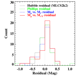
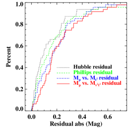
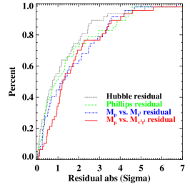
Figure 2.— Histogram (left panel) and cumulative (middle panel) distributions of the residuals, and the absolute value of the residual (residual divided by the uncertainty; right panel) distribution for the four cases (the three relations shown in Figure 1 plus Hubble residuals from MLCS2k2 fitting) for “group1.” The residuals are generally comparable.

Figure 3.— Histogram distribution of the $\chi^{2}$ difference between the $M_{p}$ vs. $M_{v^{2}t^{2}}$ relation and the others, from bootstrap simulations (see text for details). A residual difference less than zero indicates that the $M_{p}$ vs. $M_{v^{2}t^{2}}$ relation is better than the comparison. For 1000 simulations, the statistical probability (given by the percentage in each panel) shows that the $M_{p}$ vs. $M_{v^{2}t^{2}}$ relation is clearly better than the Phillips relation and the $M_{p}$ vs. $M_{t^{2}}$ relation, and it is essentially as good as the MLCS2k2 fitting method.

Although the $M_{p}$ vs. $M_{v^{2}t^{2}}$ relation does not show improvements compared to the other three methods, they may have ($M_{p}$ vs. $M_{t^{2}}$ and $M_{p}$ vs. $M_{v^{2}t^{2}}$) a linear functional form. Unlike the Phillips relation, which becomes nonlinear at the faint end where most objects are subluminous SNe Ia like SN 1991bg (e.g., Filippenko et al. 1992) having large ${\Delta}m_{15}(B)$ values, the new relation is linear throughout the entire abscissa range. This can be directly read from Equation 5, which also gives a probable physical explanation for the new relation.

4.2. Subgroups from the Full Sample

In the above analysis, we selected SNe Ia with very loose criteria; the only two cuts were to exclude objects at $z<0.005$ and objects with host-galaxy extinction $E(B-V)>0.3$ mag. Application of tighter constraints could likely reduce the scatter. For example, SNe Ia with large ${\Delta}m_{15}(B)$ are thought to be outliers from the Phillips relation, and should therefore be excluded. Also, a more stringent extinction cut could improve the fit. Here, we study several subgroups from the full sample and examine their properties.

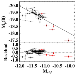
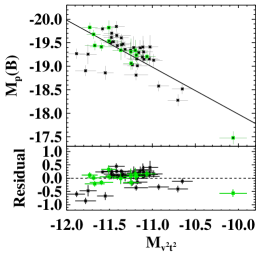
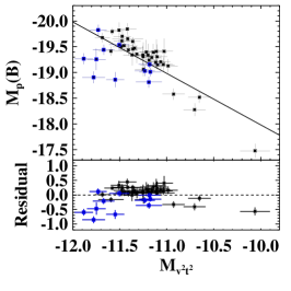
Figure 4.— Same as the right panel in Figure 1 for the new $M_{p}$ vs. $M_{v^{2}t^{2}}$ relation in Equation 5, but overplotted with different subgroups. Left panel: red points show the SNe Ia with large ${\Delta}m_{15}(B)$, which usually do not follow the Phillips relation, but they generally follow the new $M_{p}$ vs. $M_{v^{2}t^{2}}$ relation. Middle panel: green points show the SNe Ia with medium host-galaxy extinction ($0.1<E(B-V)<0.3$ mag). Right panel: blue points show SNe Ia having high photospheric velocity, $v_{{\rm Si~{}II}~{}\lambda 6355}\geq 12.0$k km s^-1 at peak brightness. They appear to be systematically below the best-fit relation.

First, we consider those SNe Ia with ${\Delta}m_{15}(B)>1.6$ mag, which usually do not follow the Phillips relation well (e.g., Taubenberger 2017). They are shown as red points in the left panel of Figure 4. It is noteworthy that they generally follow the new $M_{p}$ vs. $M_{v^{2}t^{2}}$ relation, though they are typically outliers in the Phillips relation. This means that with the new relation, it is possible to compare them with normal SNe Ia. However, these SNe are generally below the best-fitting result for the new relation, indicating that they are likely intrinsically underluminous — consistent with the fact that most of them are underluminous SN 1991bg-like SNe Ia.

Next, we examine SNe with different host-galaxy extinctions. Since the new relation cannot help derive the host extinction, we use the value estimated from the MLCS2k2 fitting, and we exclude the SNe having large extinction ($E(B-V)>0.3$ mag) in the above studies. Here we examine those SNe with medium host extinction ($0.1<E(B-V)<0.3$ mag), which are shown as green points in the middle panel of Figure 4. As one can see, these objects spread out in our sample with large scatter, consistent with the fact that they have relatively large unknown host-galaxy extinction.

Figure 5.— Histogram (left panel) and cumulative (right panel) distributions of the Si II $\lambda$6355 velocity at the time of peak brightness for the “group1” sample.

Lastly, we also examine the SNe with different Si II $\lambda$6355 velocity at peak brightness. Wang et al. (2009; 2013) and Foley & Kasen (2011) grouped high- and normal-velocity SNe Ia based on a photospheric velocity boundary of 11.8k km s^-1 at peak brightness. Interestingly, they found that the $B-V$ color at maximum brightness of high-velocity SNe Ia is redder by $\sim 0.1$ mag on average. Wang et al. (2013) also found that SNe Ia with high velocity ($v_{{\rm Si~{}II}~{}\lambda 6355}\geq 12.0$k km s^-1 at peak brightness) are substantially more concentrated in the inner and brighter regions of their host galaxies than are normal-velocity SNe Ia, and the former tend to inhabit larger and more-luminous hosts. Figure 5 shows the histogram and cumulative distributions of the Si II $\lambda$6355 velocity at peak brightness for our “group1” sample. Although our sample is not sufficiently large for a double-Gaussian fit like that of Wang et al. (2013, see their Figure 1$c$), the high-velocity sample (with $v_{{\rm Si~{}II}~{}\lambda 6355}\geq 12.0$k km s^-1 at peak brightness), which constitutes $\sim 1/4$ of our “group1” sample, is clearly distinct from the normal-velocity sample ($v_{{\rm Si~{}II}~{}\lambda 6355}<12.0$k km s^-1). In the right panel of Figure 4, blue points show the high-velocity SNe Ia ($v_{{\rm Si~{}II}~{}\lambda 6355}\geq 12.0$k km s^-1). There is a distinct difference between the two groups: the high-velocity SNe lie systematically below the best-fit $M_{p}$ vs. $M_{v^{2}t^{2}}$ relation, which means they are probably intrinsically fainter than the normal-velocity SNe Ia, if not suffering higher host-galaxy extinction. The higher velocities might possibly be produced by relatively younger and more metal-rich progenitors restricted to galaxies with substantial chemical evolution, as suggested by Wang et al. (2013).

It is interesting to see that both subsamples with ${\Delta}m_{15}(B)>1.6$ mag (left panel of Figure 4) and with $v_{{\rm Si~{}II}~{}\lambda 6355}\geq 12.0$k km s^-1 (right panel of Figure 4) are systematically below the best-fit $M_{p}$ vs. $M_{v^{2}t^{2}}$ relation, probably indicating that they are intrinsically fainter than the normal SNe Ia. Our method provides a possible way to distinguish these subluminous SNe Ia from the normal ones.

4.3. The Low-Velocity Golden Sample

Figure 6.— Same as Figure 1, but for the “group2” sample with tighter selection critera; see text for details. Compared to Figure 1, the scatter in each relation has improved significantly. In particular, the improvement for the new $M_{p}$ vs. $M_{v^{2}t^{2}}$ relation (right panel) is much more significant than that for the others.

In the above section, we show that some subgroups of SNe Ia are outliers to one or all of the relations, and some are systematically offset from the best-fit relations. In order to make a better and more stringent comparison between the different relations, we adopt an even smaller set of $z>0.005$ SNe Ia by excluding those with ${\Delta}m_{15}(B)>1.6$ mag, those with host extinction $E(B-V)>0.1$ mag, and those with $v_{{\rm Si~{}II}~{}\lambda 6355}\geq 12.0$k km s^-1 at peak brightness. This set has 22 SNe Ia (out of the 47 in “group1”), which we call the “low-$v$ golden sample” and label as “group2” for comparison with further restricted subsets. This smaller, but more homogeneous, low-$v$ golden sample minimizes the effects of host-galaxy extinction and other factors (e.g., we exclude outliers to the Phillips relations), and can therefore better reveal relations between parameters.

Similar to “group1,” we apply the analysis again to compare the four cases (three different relations, as well as the Hubble residuals from MLCS2k2 fitting) to this low-$v$ golden sample; the results are listed in Table 2 and shown in Figures 6–8.

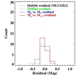
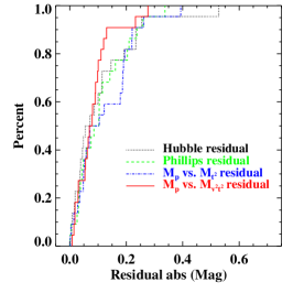
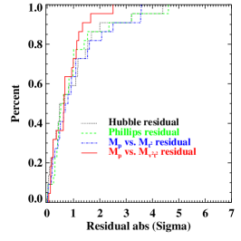
Figure 7.— Same as Figure 2, but for “group2.” The cumulative distribution clearly shows that the residuals from the new $M_{p}$ vs. $M_{v^{2}t^{2}}$ relation (red curve in the middle and right panels) are the smallest.

Figure 8.— Same as Figure 3, but for “group2.” The statistical probability shows that the new $M_{p}$ vs. $M_{v^{2}t^{2}}$ relation is much better than all others.

The residual scatter and reduced $\chi^{2}$ of all relations are improved with the smaller low-$v$ golden sample (“group2”) compared with the full sample (“group1”), as seen from Figure 6 and Table 2. In the case of the “group1” sample, the residual scatters are larger than 0.26 mag for all four cases, while for “group2,” the residuals are now all around or below 0.17 mag. This result is shown in Figure 7, where the left panel shows the histogram distributions of the residuals for all four cases and the right panel displays the corresponding cumulative distributions for “group2.” The reduced $\chi^{2}$ values are also substantially decreased: for “group1,” all are higher than 3.4, while now for “group2,” all become smaller than 2.3.

When we use the AIC_c to perform model selection with the “group2” sample, we find very strong positive evidence in favor of $M_{p}$ vs. $M_{v^{2}t^{2}}$ ($\Delta{\rm AIC}_{c}\approx 27$), as shown in Table 2. Indeed, while all four relations have similar scatter for “group1,” the new $M_{p}$ vs. $M_{v^{2}t^{2}}$ relation yields the smallest scatter among the four cases for “group2”, with a residual of only $0.108\pm 0.018$ mag, which is $\sim 0.05$ mag smaller than the other three cases.

This is confirmed by the residual cumulative distributions for the new $M_{p}$ vs. $M_{v^{2}t^{2}}$ relation (red curve in the right panel of Figure 7), which clearly stands out at the left edge (i.e., smaller residuals).

We once again use a bootstrap procedure to additionally compare the models as in Section 4.1, but now applying it to “group2.” For 1000 simulations, as shown in Figure 8, the statistical probability is 94.6%, 99.3%, and 90.6% better than the Phillips relation, the $M_{p}$ vs. $M_{t^{2}}$ relation, and the MLCS2k2 fitting method, respectively.

Although we have removed peculiar velocities expected from the Carrick et al. (2015) model, we expect that the model is imperfect. There should be significant residual scatter arising from peculiar velocities of $\sim 250$ km s^-1. We note that we have not removed this contribution from the residual scatter we have presented in this paper. Our residual from the new $M_{p}$ vs. $M_{v^{2}t^{2}}$ relation for “group2” is only $0.108\pm 0.018$ mag. If we adopt a median residual peculiar-velocity uncertainty of $\pm 250$ km s^-1, corresponding to 0.11 mag, we conclude that the measured residual scatter for the new $M_{p}$ vs. $M_{v^{2}t^{2}}$ relation is likely dominated by the peculiar-velocity uncertainty. A more precise Monte Carlo simulation, as in Section 4.1, gives a scatter of $0.135\pm 0.030$ mag with an average peculiar velocity of $\pm 250$ km s^-1 applied to this low-$v$ golden sample. We note that we obtain a similar intrinsic scatter if we do not remove peculiar velocities expected from the Carrick et al. (2015) model, and assume a scatter arising from peculiar motions of 300 km s^-1.

Another factor that may contribute to the final scatter is the temperature of SNe Ia at the time of peak brightness. In Equation 3, we assume that SNe Ia all have the same temperature at peak brightness, but this is not actually true. If the temperature among SNe Ia varies by 10%, this will contribute $\sim 0.1$ mag to the final scatter, assuming optical passbands lie on the Rayleigh-Jeans tail of SN spectra. For extreme cases, comparing the SN 1991bg-like SNe Ia with SN 1991T-like SNe Ia, adopting temperatures from Nugent et al. (1995) could cause a 0.43 mag difference. On average, SN 1991bg-like SNe Ia are $\sim 0.22$ mag fainter than normal SNe Ia, which could partially explain why SN 1991bg-like SNe Ia are generally below the best-fit line in Figure 4 (left panel), but cannot explain the high-velocity SNe Ia that are also below the best-fit line in Figure 4 (right panel). Note that previous works have found (e.g., Wang et al. 2009; Foley et al. 2011; Blondin et al. 2012; Mandel et al. 2014) that high-velocity SNe Ia are likely intrinsically redder (lower temperature) than normal-velocity SNe Ia, but the difference is too small to account for the $\sim 0.4$ mag we see in the residual in Figure 4 (right panel). On the other hand, as discussed earlier, the $B$ filter has a central wavelength that is too blue to fall on the Rayleigh-Jeans tail, so the SN Ia luminosity would increase much more rapidly than linearly with the temperature as we assumed; in that case, the difference caused by the temperature would become much larger than indicated above. Therefore, we cannot completely rule out the possibility that temperature differences are responsible for the offsets of high-velocity SNe Ia. Moreover, a blackbody is not expected to provide an accurate model for the SN emission near maximum light. Since the scatter caused by the temperature is included in the final dispersion, it is difficult to distinguish this component without detailed modeling to derive the temperature, which is beyond the scope of this paper.

We note that the MLCS2k2 estimate of $A_{V}$ may also compensate for color variation intrinsic to the SN, that may result from temperature variation. We attempt to estimate the scatter from the temperature contribution by searching for correlations between the residual and the color at peak brightness (e.g., $B-V$), but we do not see any clear trend in our sample. It is possible that independent constraints on the effective temperature of the SN photosphere could be helpful in improving the calibration, and to disentangling the effect of intrinsic color variation and dust extinction (see, e.g., Scolnic et al. 2014; Mandel et al. 2016).

4.4. Subgroups in the Low-Velocity Golden Sample

As discussed above, the dispersion in inferred SN distances arising from the residual peculiar velocities likely contributes substantially to the final scatter. The scatter contributed by peculiar velocities, however, should decrease with increasing redshift. To assess this expectation, we divide the low-$v$ golden sample into a few subgroups. For “group3,” we select only SNe with $z>0.010$ from “group2” ($z>0.005$). Similarly, we select a “group4” sample with $z>0.015$ and a “group5” sample with $z>0.020$. We applied the same analysis as for “group2” and list the results in Table 2. They confirm that the scatter from the peculiar velocities decreases from “group2” to “group5” as the sample redshift increases (Figure 9). In general, the scatter for all of the relations decreases as the sample redshift increases; however, the new $M_{p}$ vs. $M_{v^{2}t^{2}}$ relation gives the best result (smallest scatter) among the four cases. This is clearly shown in Table 2 by the AIC_c statistic comparison (for our cases, since the number of parameters is the same, comparing AIC_c is equivalent to comparing the $\chi^{2}$ value). For “group3,” “group4,” and “group5,” the difference between the AIC_c value for $M_{p}$ vs. $M_{v^{2}t^{2}}$ and the other relations is at least 6, which indicates significant positive evidence. The bootstrap simulations yield a consistent, if less significant, result: the $M_{p}$ vs. $M_{v^{2}t^{2}}$ relation yields smaller scatter for 93.3%, 78.7%, and 79.3% of bootstrap realizations than the Phillips relation for “group3,” “group4,” and “group5,” respectively. As compared with the MLCS2k2 method, the probability is 89.5%, 85.8%, and 68.1% better (respectively); however, we note that the sample sizes for group4 and group5 are relatively small.

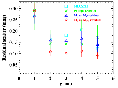
Figure 9.— The residual scatter for the low-$v$ golden sample changes with redshift cutoff from “group2” ($z>0.005$) through “group5” ($z>0.020$). Also shown is the result for the full sample of “group1.”

5. Discussion

Table 3Fitting Comparison

Groups	$\chi^{2}$	AICc	$\chi^{2}$	AICc
	Phillips relation
	$k=3$		$k=1$
group1	217.23	223.79	240.00	242.09
group2	41.49	48.52	47.42	49.62
group3	40.36	47.96	46.11	48.35
group4	36.79	45.19	41.49	43.82
group5	18.52	32.52	34.08	36.88
	$M_{p}$ vs. $M_{v^{2}t^{2}}$ relation
	$k=2$		$k=1$
group1	262.26	266.53	263.27	265.36
group2	18.34	22.97	19.35	21.55
group3	16.86	21.61	18.40	20.64
group4	15.34	20.43	17.46	19.79
group5	7.08	14.08	8.61	11.41

Our results are robust to the specific choice of sample extinction, redshift, and velocity cuts that we adopt. Wang et al. (2009, 2013) and Foley & Kasen (2011) apply similar photospheric velocity cuts to study populations of low- and high-velocity SNe.

We note that there is an outlier, SN 2000dn, quite far away from the Phillips relation. This SN is more consistent with the new $M_{p}$ vs. $M_{v^{2}t^{2}}$ relation. To test whether our results were robust to excluding this SN, we refit all the group samples after removing it. Table 4 shows the $\chi^{2}$ results for comparison. The $M_{p}$ vs. $M_{v^{2}t^{2}}$ relation still offers significant improvement when compared to the Phillips relation for “group2” and “group3,” although we find no difference for the smaller “group4” and “group5” samples.

Table 4$\chi^{2}$ Fitting Results After Excluding SN 2000dn

Groups	Hubble residual	Phillips	$M_{p}$ vs. $M_{t^{2}}$	$M_{p}$ vs. $M_{v^{2}t^{2}}$
group1	148.15	225.96	232.39	262.32
group2	35.34	23.97	33.04	17.35
group3	35.25	22.06	31.49	16.51
group4	33.01	15.76	27.54	15.46
group5	4.24	7.90	8.61	6.62

6. Conclusions

From the above analysis for both the “group1” and “group2” samples, we obtain the following conclusions.

(1) The $M_{p}$ vs. $M_{v^{2}t^{2}}$ relation yields the most precise distances among the four models considered for the low-$v$ golden sample.

(2) The new $M_{p}$ vs. $M_{v^{2}t^{2}}$ relation is mathematically linear, as shown in Equation 5; this offers a useful simplification compared to the quadratic Phillips relation.

(3) The rise time $t_{r}$ is probably better than the decay-time parameter ${\Delta}m_{15}(B)$ for studying SNe Ia. Both the $M_{p}$ vs. $M_{v^{2}t^{2}}$ and the $M_{p}$ vs. $M_{t^{2}}$ relations are comparable to (or much better than) the Phillips relation; moreover, they are easier to explain with linear formulas (Equations 5 and 6).

(4) The photospheric velocity plays an important role in improving estimates of SN Ia luminosities within our model. Comparing the $M_{p}$ vs. $M_{t^{2}}$ relation (without considering the photospheric velocity) with the new $M_{p}$ vs. $M_{v^{2}t^{2}}$ relation (considering the photospheric velocity), we see that the latter is significantly better than the former, especially for the “group2” samples.

(5) We also confirm that high-velocity SNe Ia are probably intrinsically different from normal-velocity SNe Ia, consistent with the conclusions of other groups (Wang et al. 2009, 2013; Foley & Kasen 2011). We show that high-velocity SNe Ia are probably intrinsically fainter than the normal-velocity SNe Ia.

In the future, the new $M_{p}$ vs. $M_{v^{2}t^{2}}$ relation can potentially be extended to higher redshifts. If the SN light curves are well observed, then the first-light times can be estimated with the method presented by Zheng & Filippenko (2017) and Zheng at al. (2017). This may lead to another way of determining SN distances and be used for cosmology (e.g., Jha et al. 2007; Guy et al. 2007). Since our method relies on the estimate of first-light time, it is very important to obtain a good light-curve sample in the $B$ (or $g$) band. Our suggestion for future surveys is to perform high-cadence photometry (ideally daily, if possible, or at least every other day), and to obtain at least one spectrum near maximum light.

To conclude, we have examined a new three-parameter relationship in Type Ia SNe: peak magnitude, rise time, and photospheric velocity. This $M_{p}$ vs. $M_{v^{2}t^{2}}$ relation is based on observations, though it is motivated by (and physically easy to explain with) the simple fireball model. We compared it with other SN Ia relations and found smaller scatter; thus, it has the potential to be used for accurate cosmological distance determinations.

References

- (1) Akaike, H. 1974, IEEE Trans. Automat. Control., 19, 716
- (2) Blondin S., Mandel, K. S., & Kirshner, R. P. 2011, A&A, 526, 81
- (3) Blondin S., Matheson, T., Kirshner, R. P., et al., 2012, AJ, 143, 126
- (4) Branch, D., Dang, L. C., Hall, N., et al., 2006, PASP, 118, 560
- (5) Burns, C. R., Stritzinger, M., Phillips, M. M., et al., 2014, ApJ, 789, 32
- (6) Carrick, J., Turnbull, S. J., Lavaux, G., & Hudson, M. 2015, MNRAS, 450, 317
- (7) Childress M., Aldering, G., Antilogus, P., et al. 2013, ApJ, 770, 108
- (8) Conley, A., Goldhaber, G., Wang, L., et al., 2006, ApJ, 644, 1
- (9) Contreras, C., Hamuy, M., Phillips, M. M., et al. 2010, ApJ, 139, 519
- (10) Elias-Rosa N., Benetti, S., Cappellaro, E., et al., 2006, MNRAS, 369, 1880
- (11) Fakhouri, H. K., Boone, K., Aldering, G., et al. 2015, ApJ, 815, 58
- (12) Filippenko A. V. 1997, ARA&A, 35, 309
- Filippenko et al. (2001) Filippenko A. V., Li W. D., Treffers R. R., Modjaz M. 2001, in Small-Telescope Astronomy on Global Scales., ed. B. Paczyński, W. P. Chen, & C. Lemme (San Francisco: ASP), 121
- Filippenko et al. (1992) Filippenko A. V., Richmond M. W., Branch D., et al. 1992, AJ, 104, 1543
- (15) Folatelli G., Morrell, N., Phillips, M. M., et al., 2013, ApJ, 773, 53
- (16) Foley R. J., & Kasen, D. 2011, ApJ, 729, 55
- (17) Ganeshalingam, M., Li, W., Filippenko, A. V., et al. 2010, ApJS, 190, 418
- (18) Ganeshalingam M., Li, W., Filippenko, A. V., et al. 2012, ApJ, 751, 142
- (19) Garnavich P., 2008, CBET, 1558, 1
- (20) Guy J., Astier, P., Nobili, S., et al. 2005, A&A, 443, 781
- (21) Guy, J., Astier, P., Baumont, S., et al. 2007, A&A, 466, 11
- (22) Hamuy M., Phillips, M. M., Wells, L. A., et al. 1993, PASP, 105, 787
- (23) Hicken, M., Challis, P., Jha, S., et al., 2009a, ApJ, 700, 331
- (24) Hicken M., Wood-Vasey, W. M., Blondin, S., et al. 2009b, ApJ, 700, 1097
- (25) Jha, S., Riess, A. G., Kirshner, R. P. 2007, ApJ, 659, 122
- (26) Kass, R. E., & Raftery, A. E. 1995, J. Am. Stat. Assoc., 90, 773
- (27) Kelly P. L., Hicken, M., Burke, D. L., et al. 2010, ApJ, 715, 743
- (28) Kelly P. L., Filippenko, A. V., Burke, D. L., et al. 2015, Science, 347, 1459
- (29) Lampeitl H., Smith, M., Nichol, R. C., et al. 2010, ApJ, 722, 566
- (30) Leaman J., Li W., Chornock R., Filippenko A. V. 2011, MNRAS, 412, 1419
- (31) Maguire, K., Sullivan, M., Thomas, R. C., et al. 2011, MNRAS, 418, 747
- (32) Mandel, K. S., Foley, R. J. & Kirshner, R. P., 2014, 797, 75
- (33) Mandel, K. S., Scolnic, D., Shariff, H., et al. 2016, ApJ, 842, 93
- Markwardt (2009) Markwardt C. B. 2009, Astronomical Data Analysis Software and Systems XVIII, 411, 251
- (35) Mukherjee, S., Feigelson, E. D., Jogesh, B., et al. 1998, ApJ, 508, 314
- (36) Nugent P., Phillips, M., Baron, E., et al., 1995, ApJL, 455, L147
- (37) Nugent P. E., Kim, A., & Perlmutter, S. 2002, PASP, 114, 803
- (38) Perlmutter, S., Aldering, G., Goldhaber, G., et al. 1999, ApJ, 517, 565
- (39) Phillips, M. M. 1993, ApJ, 413, L105
- (40) Phillips M. M., Lira, P., Suntzeff, N. B., et al. 1999, AJ, 118, 1766
- (41) Phillips M. M., Li, W., Frieman, J. A., et al., 2007, PASP, 119, 360
- (42) Rigault M., Copin, Y., Aldering, G., et al. 2013, A&A, 560, 66
- (43) Rigault M., Aldering, G., Kowalski, M., et al. 2015, ApJ, 802, 20
- (44) Riess, A. G., Press, W. H., & Kirshner, R. P. 1996, ApJ, 473, 88
- (45) Riess, A. G., Filippenko, A. V., Challis, P., et al. 1998, AJ, 116, 1009
- (46) Riess A. G., Filippenko, A. V., Li, W., et al. 1999, AJ, 118, 2675
- (47) Schlafly, E. F. & Finkbeiner, D. P., 2011, ApJ, 737, 103
- Schlegel et al. (1998) Schlegel, D. J., Finkbeiner, D. P., & Davis, M. 1998, ApJ, 500, 525
- (49) Scolnic, D. M., Riess, A. G., Foley, R. J., et al. 2014, ApJ, 780, 37
- (50) Silverman J. M., Kong, J. J., Filippenko, A. V., et al. 2012, MNRAS, 425, 1819
- (51) Silverman J. M., Vinkó, J., Marion, G. H., et al. 2015, MNRAS, 451, 1973
- (52) Sugiura, N. 1978, Commun. Stat. A-Theor., 7, 13
- (53) Sullivan M., Conley, A., Howell, D. A., et al. 2010, MNRAS, 406, 782
- (54) Taubenberger, S., 2017, arXiv:1703.00528
- (55) Tripp R. 1998, A&A, 331, 815
- (56) Wang L., Goldhaber, G., Aldering, G., et al. 2003, ApJ, 590, 944
- (57) Wang X., Filippenko, A. V., Ganeshalingam, M., et al. 2009, ApJ, 699, 139
- (58) Wang X., Wang, L., Filippenko, A. V., et al. 2013, Science, 340, 170
- (59) Wang X., Wang, L., Zhou, X., et al. 2005, ApJ, 620, L87
- (60) Zheng, W., & Filippenko, A. V. 2017, ApJL, 838, L4
- (61) Zheng, W., Kelly, P. L., & Filippenko, A. V. 2017, ApJ, 848, 66