TrackerBots: Autonomous UAV for Real-Time Localization and Tracking of Multiple Radio-Tagged Animals

Abstract

Autonomous aerial robots provide new possibilities to study the habitats and behaviors of endangered species through the efficient gathering of location information at temporal and spatial granularity not possible with traditional manual survey methods. We present a novel autonomous aerial vehicle system—TrackerBots—to track and localize multiple radio-tagged animals. The simplicity of measuring the received signal strength indicator (RSSI) values of very high frequency (VHF) radio-collars commonly used in the field is exploited to realize a low cost and lightweight tracking platform suitable for integration with unmanned aerial vehicles (UAVs). Due to uncertainty and the non-linearity of the system based on RSSI measurements, our tracking and planning approaches integrate a particle filter for tracking and localizing and a partially observable Markov decision process (POMDP) for dynamic path planning. This approach allows autonomous navigation of a UAV in a direction of maximum information gain to locate multiple mobile animals and reduce exploration time; and, consequently, conserve on-board battery power. We also employ the concept of a search termination criteria to maximize the number of located animals within power constraints of the aerial system. We validated our real-time and online approach through both extensive simulations and field experiments with five VHF radio-tags on a grassland plain.

1 Introduction

Understanding basic questions of ecology such as how animals use their habitat, their movements and activities are necessary for addressing numerous environmental challenges ranging from invasive species to diseases spread by animals and saving endangered species from extinction. Conservation biologists, ecologists as well as natural resource management agencies around the world rely on numerous methods to monitor animals. Traditional methods using radio-tagging species of interest [Cochran and Lord Jr, 1963, Kenward, 2000] as well as more recent vision-based sensors [Selby et al., 2011, Olivares-Mendez et al., 2015] or infrared (IR) based sensors [Zhou, 2013, Christiansen et al., 2014, Gonzalez et al., 2016, Ward et al., 2016] are employed for these tasks. IR-based sensors are sensitive to environmental temperature and become less reliable when they are used outdoors, especially during day-times in summer months [Zhou, 2013]. In general, vision-based approaches are less effective when animals are camouflaged and are susceptible to visual occlusions, e.g. by grass, shrubs and even other animals. Most significantly, due to the difficulty of automatically recognizing individual animals using vision/IR based approaches, tracking multiple animals with these sensors require dealing with the very challenging problem of data association [Bar-Shalom, 1987, Stone et al., 2013]. Often, conservation biologists need tools to track and monitor a specific set of individual animal species; for example, individuals of a reintroduction species into a natural habitat. This becomes difficult to achieve in the presence of occlusions and data associations problems of IR/vision based approaches. Thus, capturing and collaring concerned species with Very High Frequency (VHF) radio tags and the subsequent use of VHF telemetry or radio tracking is the most important and cost-effective tool employed to study the movement of a wide range of animal sizes [Wikelski et al., 2007] in their natural environments [Kays et al., 2011, Thomas et al., 2012, Tremblay et al., 2017, Webber et al., 2017].

However, the traditional method of radio tracking is not without its problems. Tracking radio-collared animals typically requires researchers to trek long distances in the field, armed with cumbersome VHF radio receivers with hand-held antennas and battery packs to manually home in on radio signals emitted from radio-tagged or collared animals. Consequently, the precious spatial data acquired through radio tracking come at a significant cost to researchers in terms of manpower, time and funding. The problem is often compounded by other challenges, such as low animal recapture rates, equipment failures, and the inability to track animals that move into inaccessible terrains. Furthermore, many of our most endangered species also happen to be the most difficult to track due to their small size, inconspicuousness, and location in remote habitats.

Automated tracking and location of wildlife with autonomous unmanned aerial vehicles (UAVs) can provide new possibilities to better understand ecology and our native wildlife to safeguard biodiversity and manage our natural resources cost-effectively. We present a low-cost approach capable of realization in a lightweight payload for transforming existing commodity drone platforms into autonomous aerial vehicle systems as shown in Fig. 1 to empower conservation biologists to track and localize multiple radio-tagged animals.

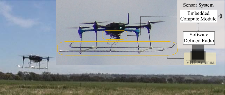
Figure 1: TrackerBots: An overview of the UAV tracking platform with its sensor system.

The main contribution of our work is a new autonomous aerial vehicle system for simultaneously tracking and localizing multiple mobile radio-tagged animals using VHF radio-collars, commonly used in the field. In particular:

• Our system is realized in a 260 g payload suitable for a multitude of low-cost, versatile, easy to operate multi-rotor UAVs. Our lightweight realization—of less than 2 kg system mass—is achieved through a new sensor design that exploits the simplicity of a software-defined radio architecture for capturing received signal strength indicator (RSSI) value from multiple VHF radio tags and a compact, lightweight VHF antenna geometry. The lightweight design is significant for achieving longer flight times on a given UAV as well as making the technology more accessible in jurisdictions, such as Australia, where systems under 2 kg can be flown without a pilot license.

• We formulate a joint tracking and path planning problem to realize a real-time and online autonomous system. Due to the noisy, complex and nonlinear characteristics of RSSI data, we integrate a sequential Monte Carlo implementation of a Bayesian filter, also known as particle filter (PF), for real-time tracking and localization jointly with a partially observable Markov decision process (POMDP) for modeling a path planning decision process. We evaluate information based reward functions to evaluate control actions for path planning. We use Réyni divergence between prior and posterior estimates of target locations for autonomy and dynamic online path planning to minimize flight time while maximizing the number of located animals. Further, our formulation considers the trade-off between location accuracy and resource constraints of the UAV, its maneuverability, and power constraints to develop a practical solution.

• We validate our method through extensive simulations and field experiments with mobile VHF radio-tags. In particular, we conducted: i) over 10 manual flights to both evaluate and measure the performance of our sensor system; and ii) we performed 20 autonomous flights under two different settings with a mix of target dynamics to demonstrate the robustness and scalability of our approach. To the best of our knowledge, ours is the first demonstration of an autonomous online aerial robot system for tracking and locating multiple mobile VHF radio-tags in real-time.

• In order to support researchers in the field and facilitate the adoption of new technologies in the field, we provide a complete design description of TrackerBots, including a repository of source code to develop our fully autonomous system 

2 Related Work

Our problem is embedded in the development of a UAV planning method for tracking multiple mobile radio-tagged objects using the simplicity of received signal strength measurements. Therefore: i) we review studies in the field of received signal strength measurement based tracking with a specific focus on methods developed for UAVs and wildlife tracking; ii) we review multi-target tracking methods since our problem involves tracking multiple radio-tagged targets; and iii) we focus on related work in the field of tracking radio-collared animals using UAVs.

Received signal strength indicator (RSSI)-based Tracking: This method is studied in localizing objects in both indoor and outdoor environments. The approach relies on using the strength of a radio signal from an emitter captured by a receiver to estimate, for example, the distance to the emitter. Related methods with possible applications to wildlife tracking can be found in the use of wireless sensor networks (WSN) for tracking a radio wave emitter. In [Caballero et al., 2008, Särkkä et al., 2014] a mobile beacon is localized by a fixed number of sensor nodes with known locations. The first automated VHF telemetry measurement system was reported in [Kays et al., 2011]. A set of six ground-based antenna arrays deployed in a rainforest localized radio-tagged animal locations using bearing estimates obtained from signal strength measurements made by ground-based stations. These methods are advantageous for meeting long-term monitoring needs. However, the scale of the fixed and powered infrastructure required prior to a tracking task and the cost of deployment and maintenance over a large area make these approaches difficult for general use cases. In contrast, a UAV based measurement method can provide greater flexibility and a lower cost approach. Off-line estimations of a radio-tag’s location obtained from signal strength data logged from a UAV was demonstrated in [Jensen et al., 2014]. Developments in Software-defined radios (SDRs) have enabled new capabilities to process multiple radio-tag signals simultaneously. Early efforts to demonstrate the possibility of incorporating SDR architectures with a UAV to detect multiple transmitted signals from radio-tags were reported in [Dos Santos et al., 2014, VonEhr et al., 2016]. Notably, the studies above with UAVs were performed under the assumption of stationary radio tags. The task of autonomously tracking and locating multiple mobile radio-tagged targets from a UAV remains.

Multi-target Tracking: The objective of multi-target tracking is to accurately estimate the unknown state of multiple objects or targets using noisy observations. The basic problem in multi-target tracking is the unknown associations between measurements and targets [Bar-Shalom, 1987]. Traditional multi-target tracking formulations include multiple hypotheses tracking (MHT) filter [Blackman, 1986], the joint probabilistic data association filter (JPDAF) [Bar-Shalom, 1987], and the probabilistic MHT (PMHT) filter [Streit and Luginbuhl, 1994]. These approaches require explicit associations between measurements and targets and propagate these hypotheses over time [Vo and Ma, 2006]. Another alternative approach which obviates explicit data associations uses finite set statistics (FISST) proposed by Mahler based on Random Finite Set (RFS) theory. This formulation has gained considerable interest in recent years and has lead to a number of new filtering solutions such as the probability hypothesis density (PHD) filter [Mahler, 2003], the cardinalized PHD (CPHD) filter [Mahler, 2007a], the multi-object multi-Bernoulli (MeM-Ber) filter [Mahler, 2007b, Vo et al., 2009], the labeled multi-Bernoulli (LMB) filter [Reuter et al., 2014], and the generalized labeled multi-Bernoulli (GLMB) filter [Vo and Vo, 2013, Vo et al., 2014]. Since the radio-tagged methods provide an elegant solution where each target can be uniquely identified by its transmitted signal, our problem does not suffer from the data association problems mentioned above. Thus, we propose formulating a Particle Filter (PF)  [Gordon et al., 1993] for tracking radio-tags. This is similar to the approach in  [Charrow et al., 2015]. In contrast to the simulation-based study of indoor robots in [Charrow et al., 2015], we design and implement our algorithm on a UAV with a sensor system for obtaining RSSI-based measurements of multiple radio-tagged objects in outdoor environments.

UAV-based Autonomous Localization and Tracking: Since this application is related to locating VHF collared animals, we will focus on progress made towards the autonomous localization and tracking of multiple VHF radio-tagged animals here.

Pioneering achievements in autonomous wildlife tracking have been made through simulation studies [Posch and Sukkarieh, 2009] and experimentally demonstrated systems  [Cliff et al., 2015, Körner et al., 2010, Tokekar et al., 2010, Vander Hook et al., 2014] in recent years. In particular, the first demonstration of a UAV was presented in [Cliff et al., 2015].

The recent approaches [Cliff et al., 2015, Vander Hook et al., 2014] for real-time localization of a static target (assuming stationary wildlife) used wireless signal characteristics captured by a narrowband receiver to estimate location; in particular, the angle-of-arrival (AoA) of a radio beacon was determined using an array of antennas with the information related to a ground-based receiver for location estimations. Although the approach can conveniently manage topological variations in terrain, AoA systems require a large bulky receiver system and multiple antenna elements as well as long observation times; 45 seconds per observation as reported in [Cliff et al., 2015]. Moreover, the antenna systems being mounted on top of the UAV [Cliff et al., 2015] is likely to lead to difficulty in tracking terrestrial animals although being suitable for locating avian species dwelling in trees.

Summary: We can see that there are few investigations that have studied the problem of locating radio-collared animals using autonomous robots. Although a system based on angle-of-arrival was recently evaluated to locate a stationary animal, the development of a low-cost and lightweight autonomous system capable of long-range flights and localization of multiple mobile radio-collared animals still remains.

We present an alternative approach exploiting RSSI based measurements because of the ability to use a simpler sensing system on board commodity UAVs to realize lower cost and longer flight time UAVs for tracking and localizing multiple animals. Together with a theoretical framework for joint tracking and planning, we design, build and demonstrate a lightweight autonomous aerial robot platform. Our robot platform has the potential to provide a cost-effective method for wildlife conservation and management. To the best of our knowledge, ours is the first demonstration of an autonomous online aerial robot system for tracking and locating multiple mobile VHF radio-tags in real-time.

3 Tracking and Planning Problem Formulation

Real-time tracking requires an online estimator and a dynamic planning method. This section presents our tracking and localizing formulation under the theoretical frameworks of a Bayesian filter for tracking and POMDP for planning strategy.

3.1 Tracking and localizing

For tracking, we use a Bayesian filter. It is an online estimation technique which deals with the problem of inferring knowledge about the unobserved state of a dynamic system—in our problem, wildlife—which changes over time, from a sequence of noisy measurements. Suppose $\mathbf{x}\in\mathcal{X}$ and $\mathbf{z}\in\mathcal{Z}$ are respectively the system (kinematic) state vector in the state space $\mathcal{X}$ and the measurement (observation) vector in the observation space $\mathcal{Z}$. The problem is estimating the state $\mathbf{x}\in\mathcal{X}$ from the measurement $\mathbf{z}\in\mathcal{Z}$ or calculating the marginal posterior distribution $\mathit{p(\mathbf{x}_{\mathit{k}}|\mathbf{z}_{1:k})}$ sequentially through prediction (1) and update (2) steps.

$$\mathit{p(\mathbf{x}_{\mathit{k}}|\mathbf{z}_{\mathit{1:k-1}})} =\mathit{\int{p(\mathbf{x}_{\mathit{k}}|\mathbf{x}_{\mathit{k-1}})p(\mathbf{x}_{\mathit{k-1}}|\mathbf{z}_{\mathit{1:k-1}})d\mathbf{x}_{\mathit{k-1}}}},$$ (1)

$$\mathit{p(\mathbf{x}_{\mathit{k}}|\mathbf{z}_{1:k})} =\mathit{\dfrac{p(\mathbf{z}_{\mathit{k}}|\mathbf{x}_{\mathit{k}})p(\mathbf{x}_{\mathit{k}}|\mathbf{z}_{\mathit{1:k-1}})}{\int{p(\mathbf{z}_{\mathit{k}}|\mathbf{x}_{\mathit{k}})p(\mathbf{x}_{\mathit{k}}|\mathbf{z}_{\mathit{1:k-1}})d\mathbf{x}_{k}}}}.$$ (2)

In the case of a nonlinear system or non-Gaussian noise, there is no general closed-form solution for the Bayesian recursion and $\mathit{p(\mathbf{x}_{\mathit{k}}|\mathbf{z}_{1:k})}$ generally has a non-parametric form. Therefore, in our problem, we use a particle filter implementation as an approximate solution for the Bayesian filtering problem due to our highly nonlinear measurement model.

Particle Filter (PF): A particle filter uses a sampling approach to represent the non-parametric form of the posterior density $\mathit{p(\mathbf{x}_{\mathit{k}}|\mathbf{z}_{1:k})}$. The samples from the distribution are represented by a set of particles; each particle has a weight assigned to represent the probability of that particle being sampled from the probability density function. Then, these particles representing the non-parametric form of $\mathit{p(\mathbf{x}_{\mathit{k}}|\mathbf{z}_{1:k})}$ are propagated over time. In the simplest version of the particle filter, known as the bootstrap filter first introduced by Gordon in [Gordon et al., 1993], the samples are directly generated from the transitional dynamic model. Then, to reduce the particle degeneracy, resampling and injection techniques are implemented; a detailed algorithm can be found in [Ristic et al., 2004].

Measurement model: The update process of a PF requires the derivation of a likelihood of measurements. In our problem, based on estimating a target’s—VHF radio tag’s—range from the receiver, we require a realistic signal propagation model to obtain the likelihood of receiving a given measurement. We employ two VHF signal propagation models suitable for describing RSSI measurements in non-urban outdoor environments [Patwari et al., 2005, Jakes, 1974]. Denoting $\mathbf{h(x,u)}$ as the RSSI measurement function between target $\mathbf{x}$ and observer (UAV) state $\mathbf{u}$, we have:

i) Log Distance Path Loss Model (LogPath): The received power is the only line of sight power component transmitted from a transmitter subjected to signal attenuation such as through absorption and propagation loss [Patwari et al., 2005]:

$$\mathbf{h(x,u)}=P_{r}^{d_{0}}-10n\log_{10}(d(\mathbf{x},\mathbf{u}_{p})/d_{0})+G_{r}(\mathbf{x,u}),$$ (3)

where

• $\mathbf{x}=[p_{x}^{t},p_{y}^{t},p_{z}^{t}]^{T}$ is the target’s position; $\mathbf{u}_{p}=[p_{x}^{u},p_{y}^{u},p_{z}^{u}]^{T}$ is the observer’s (UAV) position in Cartesian coordinates; $\mathbf{u}=[\mathbf{u}_{p};\theta^{u}]$ is the UAV’s state which includes its heading angle $\theta^{u}$.

• $d(\mathbf{x},\mathbf{u}_{p})$ is the Euclidean distance between the target’s position and UAV’s position.

• $G_{r}(\mathbf{x,u})$ is the UAV receiver antenna gain which depends on its heading, its position, and target’s position (details explained in Sec. 6.2).

• $P_{r}^{d_{0}}$ is received power at a reference distance $d_{0}$.

• $n$ is the path-loss exponent that characterizes the signal losses such as absorption and propagation losses and this parameter depends on the environment with typical values ranging from 2 to 4 [Patwari et al., 2005].

ii) Log Distance Path Loss Model with Multi-Path Fading (MultiPath): The received power is composed of both line of sight power component transmitted from a transmitter and the multi-path power component reflected from the ground plane subjected to signal attenuation such as through absorption and propagation loss: [Jakes, 1974, p. 81]:

$$\mathbf{h(x,u)} =P_{r}^{d_{0}}-10n\log_{10}(d(\mathbf{x},\mathbf{u}_{p})/d_{0})$$ (4)

$$+G_{r}(\mathbf{x,u})+10n\log_{10}(|1+\Gamma(\psi)e^{-j\triangle\varphi}|),$$

where, in addition to terms in 3

• $\psi$ is the angle of incidence between the reflected path and the ground plane.

• $\Gamma(\psi)=[\sin(\psi)-\sqrt{\varepsilon_{g}-\cos^{2}(\psi)}]/[\sin(\psi)+\sqrt{\varepsilon_{g}-\cos^{2}(\psi)}]$ is the ground reflection coefficient with $\varepsilon_{g}$ is the relative permittivity of the ground.

• $\triangle\varphi=2\pi\triangle d/\lambda$ is the phase difference between two waves where $\lambda$ is the wavelength and $\triangle d=((p_{x}^{t}-p_{x}^{u})^{2}+(p_{y}^{t}-p_{y}^{u})^{2}+(p_{z}^{t}+p_{z}^{u})^{2})^{1/2}-d(\mathbf{x},\mathbf{u}).$

In non-urban environments, received power is usually corrupted by environmental noise, with the assumption that the noise is white, the total received power $\mathbf{z}=P_{r}(\mathbf{x,u})$ [dBm] is:

$$\mathbf{z} =\mathbf{h(x,u)}+\eta_{P},$$ (5)

where $\eta_{P}\sim\mathcal{N}(0,\sigma_{P}^{2})$ is Gaussian white noise with covariance $\sigma_{P}^{2}$. Notably, even if RSSI noise is not completely characterized by a white noise model, we found it practical to characterize the received noise with a white Gaussian model as shown in Fig. 7.

We use data captured in experiments using our sensor system to validate the physical sensor characteristics $G_{r}(\mathbf{x,u})$ (see Sec. 3) and $n$ defined by environmental characteristics, as well as estimate the propagation model reference power parameter $P_{r}^{d0}$ and noise $\sigma_{P}$ (see Sec.  6.2).

Measurement likelihood: Based on (5) with Gaussian noise $\eta_{P}$, the likelihood of measurement $\mathbf{z}_{k}$, given target and sensor position are $\mathbf{x}_{k}$ and $\mathbf{u}_{k}$, respectively, at time $k$ is

$$p(\mathbf{z}_{k}|\mathbf{x}_{k},\mathbf{u}_{k})\sim\mathcal{N}(\mathbf{z}_{k};\mathbf{h}(\mathbf{x}_{k},\mathbf{u}_{k}),\sigma^{2}_{P}),$$ (6)

where $\mathcal{N}(\cdot;\mu,{\color[rgb]{0,0,0}\sigma^{2}})$ is a normal distribution with mean $\mu$ and covariance $\sigma^{2}$.

3.2 Path Planning

The UAV planning problem is similar to the problem of an agent computing optimal actions under a partially observable Markov decision process (POMDP) to maximize its reward. [Kaelbling et al., 1998] have shown that a POMDP framework implements an efficient and optimal approach based on previous actions and observations to determine the true world states. A POMDP in conjunction with a particle filter provides a principled approach for evaluating planning decision to realize an autonomous system for tracking.

In general, a POMDP is described by the 6-tuple $(\mathcal{S,A,T,R,O,Z})$ where $\mathcal{S}$ is a set of both UAV and target states ($\mathbf{s}=\{\mathbf{x,u}\}\in S$), $\mathcal{A}$ is a set of UAV actions, $\mathcal{T}$ is a state-transition function $\mathcal{T}(\mathbf{s,a,s^{\prime}})=p(\mathbf{s^{\prime}|s,a})$ for a given action $\mathbf{a}$, $\mathcal{R}(\mathbf{a})$ is a reward function, $\mathcal{O}$ is a set of observations and $\mathcal{Z}$ is an observation likelihood $\mathcal{Z}(\mathbf{s,a,o})=p(\mathbf{o|s,a})$ with $\mathbf{s,s^{\prime}}\in\mathcal{S}$ is the current state and next state respectively, $\mathbf{a}\in\mathcal{A}$ is the taken action and $\mathbf{o}\in\mathcal{O}$ is the observation—i.e., measurement. The goal of a POMDP is to find an optimal policy to maximize the total expected reward $\mathbb{E}[\sum_{\kappa=k+1}^{k+H}\gamma^{\kappa-k-1}\mathcal{R}_{\kappa}(\mathbf{a}_{k})]$ where $H$ is look-ahead horizon steps, $\gamma$ is the discount factor which serves as the value difference between the current reward versus the future reward; $\mathbf{a}_{k}$ is action at time step $k$ and $\mathbb{E}[\cdot]$ is the expectation operator [Hsu et al., 2008].

The reward function can be calculated using different methods such as task-driven or information-driven strategies. When uncertainty is high, the information gain approach is preferable to reduce a target’s location uncertainty [Beard et al., 2017]; hence, we used this method to calculate our reward function. There are several approaches to evaluate information gain in robotic path planning such as Shannon entropy [Cliff et al., 2015], Kullback-Leibler (KL) divergence or Rényi divergence [Hero et al., 2008]. We adopted the approach in [Ristic, 2013, Ristic and Vo, 2010] to implement Rényi divergence as our reward function since it fits naturally with our Monte-Carlo sampling method. Here, Rényi divergence measures the information gain between prior and posterior densities [Beard et al., 2017, Ristic and Vo, 2010]:

$$\mathcal{R}^{(i)}_{k+H}(\mathbf{a}_{k}) =\dfrac{1}{\alpha-1}\log\int\begin{bmatrix}p(\mathbf{x}_{k+H}|\mathbf{z}_{1:k})\end{bmatrix}^{\alpha}\begin{bmatrix}p(\mathbf{x}_{k+H}|\mathbf{z}_{1:k},\mathbf{z}^{(i)}_{k+1:k+H}(\mathbf{a}_{k}))\end{bmatrix}^{1-\alpha}d\mathbf{x}_{k+H},$$ (7)

where $\alpha\geq 0$ is a scale factor to decide the effect from the tails of two distributions. The prior density $p(\mathbf{x}_{k+H}|\mathbf{z}_{1:k})$ is calculated by propagating current posterior particles sampled from $p(\mathbf{x}_{k}|\mathbf{z}_{1:k})$ to time $k+H$ using the prediction step (1). The posterior density $p(\mathbf{x}_{k+H}|\mathbf{z}_{1:k},\mathbf{z}^{(m)}_{k+1:k+H}(\mathbf{a}_{k}))$ where $\mathbf{z}^{(m)}_{k+1:k+H}(\mathbf{a}_{k})$ is the future measurement set that will be observed if action $\mathbf{a}_{k}\in\mathcal{A}_{k}$ is taken; this is calculated by applying both prediction (1) and update steps (2) up to time $k+H$. However, using Bayes update procedure is computationally expensive and prohibitive in a real-time setting. Instead, we implement a computationally efficient approach using a black box simulator proposed in [Silver and Veness, 2010] along with the Monte Carlo sampling approach. Hence, the problem transforms to find an optimal action $\mathbf{a}^{*}_{k}\in\mathcal{A}_{k}$ to maximize total expected reward:

$$\mathbf{a}^{*}_{k}\approx\arg\max\limits_{\mathbf{a}_{k}\in\mathcal{A}_{k}}\dfrac{1}{M_{s}}\sum_{t=k+1}^{k+H}\sum_{m=1}^{M_{s}}\gamma^{t-k}\mathcal{R}^{(m)}_{t}(\mathbf{a}_{k}),$$ (8)

where $M_{s}$ is the number of future measurements.

3.3 Multi-targets Tracking

The particle filter proposed in Sec. 3.1 can be extended to multi-target tracking (MTT). However, MTT normally deals with the complex data association problem where it is difficult to determine which measurement belongs to which target. In contrast, for our system, each target can be estimated from the measurement based on the signal frequency and tracked independently. Thus, we do not need to solve the data association problem. Notably, not all of the targets are detected due to, for example, the UAV movements, the measurement range limits imposed by propagation losses and receiver sensitivity. Therefore, if the target is not detected, the solver does not update its estimated position.

Besides maximizing the number of targets localized and tracked, we formulated a termination condition for each target to conserve UAV battery power; a target is considered localized if its location uncertainty, determined by a determinant of its particles covariance, is sufficiently small (<$N_{Th}$). Then, those found targets are forgotten to aid the solver to prioritize its computing resources on those targets with high uncertainty.

4 System Implementation

We implemented an experimental aerial robot system based on our tracking and planning formulation. An overview of the complete system is described in Fig. 2a. Our experimental system used a 3DR IRIS+ UAV platform and a new sensor system built with: i) a compact directional VHF antenna design, and ii) a software-defined signal processing module capable of simultaneously processing signals from multiple targets and remotely communicating with a ground control system for tracking and planning.

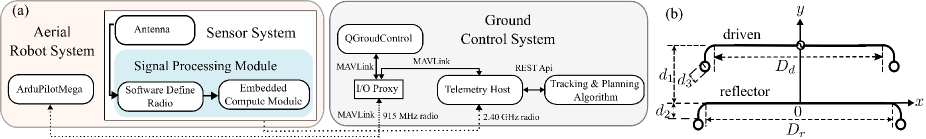
Figure 2: a) The communication channels between UAV and the ground control system with its main software components and protocols. The solid lines represent the internal connections/communications within the Sensor System and the Ground Control System. The dotted lines are connections between wireless interfaces such as the Aerial Robot System and the Ground Control System through two different radio channels: $915$ MHz and $2.4$ GHz. b) The folded 2-element Yagi antenna design used in our sensor system for observations.

In our system, the ArduPilotMega (APM) on the IRIS+ UAV transmits back its global positioning system (GPS) location to the Telemetry Host tool developed by our group to communicate with the APM module using the MAVLink protocol over a 915 MHz full duplex radio channel. The sensor system together with the antenna, SDR receiver, and the embedded compute module delivers targets’ RSSI data through a 2.40 GHz radio channel to the ground control system.

GPS locations of the UAV platform and targets’ RSSI data are delivered to our tracking and planning algorithm—solver—through the Telemetry Host using a RESTful web service. The solver estimates target locations and calculates new control actions per each POMDP cycle to command the UAV through MAVLink to fly to a new location. In order to ensure safety and meet University regulatory requirements, we also employ QGroundControl—a popular cross-platform flight control and mission planning software—to monitor and abort autonomous navigation. We detail our Sensor System below.

Signal Processing Module: Fig. 3 illustrates the components of the proposed signal processing module. We propose using a software-defined radio (SDR) receiver to implement the signal processing components. The key advantages of our choice are the ability to: i) reduce the weight of the receiver; ii) rapidly scan a large frequency spectrum to track multiple animals beaconing on different VHF frequency channels; and iii) reconfigure the system on the fly because the signal processing chain is defined in software.

In this work, we use the HackRF One SDR—an open source platform developed by [Ossmann, 2015] capable of directly converting radio frequency (RF) signals to digital signals using an analog-to-digital converter (ADC)—together with an Intel Edison board as our embedded compute module. We implemented a Discrete Fourier Transform (DFT) filter to isolate, from multiple signals, each unique VHF frequency channel associated with an animal radio collar and measure the signal strength of the received signal.

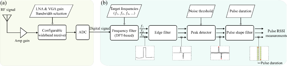
Figure 3: The signal processing module. (a) Software-defined radio: raw input RF signals are processed through the HackRF One SDR device with different configurable amplifiers–Low Noise Amplifier (LNA) and Variable Gain Amplifier (VGA), and an ADC to convert analogue signals to digital signals. (b) Embedded compute module: digital signals are processed on an Intel Edison board using a DFT (Discrete Fourier Transform)-based frequency filter with configurable input frequencies, edge filter and peak detector algorithms to derive radio collar RSSI measurements.

Antenna: A lightweight folded 2-element Yagi antenna was specially designed for our sensor system. Our design achieves a low profile antenna capable of being within the form factor of low-cost commodity UAVs suitable for easy operation in the field. Similar to a standard 2-element Yagi antenna, the folded design has one reflector and one driven element as shown in Fig. 2b.

The antenna operates in the frequency range from $145$ MHz to $155$ MHz (a typical range for wildlife radio tags), and a center frequency of $f=150$ MHz. The length of driven and reflector elements are $D_{d}=0.3975\lambda$ and $\ D_{r}=0.402\lambda$, respectively, while $d_{1}=0.1\lambda$, $d_{2}=0.03\lambda$ and the inductive loading ring diameter is $d_{3}=0.015\lambda$. Here, the wavelength $\lambda=c/f=2$ m with $c=3\cdot 10^{8}$ m/s. The antenna gain model calculated for the the design is shown in Fig. 6b.

4.1 Planning implementation for a real-time system

Implementing planning algorithms on any real-time systems is always challenging because of its high computational demand. Thus, in the following, we present the approaches to minimize the planning computational time while not sacrificing the overall localization performance:

1. Notably, for RSSI data, the uncertainty in the estimation of a target’s location is reduced when the maximum gain of the directional antenna mounted on the UAV points toward the target position. Hence, to increase the localization accuracy, the UAV heading angle $\theta^{u}_{k}$ must be controlled during the path planning process, although the multi-rotor UAV can be maneuvered without changing its heading. We select a set of discrete UAV rotation angles for the control actions $\mathcal{A}_{k}$ based on a simulation-based study to reduce the computational complexity of the POMDP planning process by limiting the number of possible actions to evaluate.

2. The solver performs planning in every $N_{p}$ observation cycles with $N_{p}>1$ instead of every observation. This approach helps to ensure that the solver prioritizes its limited computational resource on tracking targets instead of only performing planning steps.

3. A coarse planning interval $t_{p}$ in the planning procedure is implemented to minimize the computational time by reducing the number of look-ahead steps while still having the same look-ahead horizon. For example, if we want to estimate the target’s state in a 10 second horizon, we can use the normal interval $t_{p}=1$ s and estimate the target’s state 10 times or use the coarser interval $t_{p}=5$ s and perform the estimation twice; the latter approach is computationally less expensive.

4. Instead of selecting the best action from the possible action space $\mathcal{A}_{k}$, the domain knowledge of the receiver antenna gain is used to select a subset of actions that give the highest received gain using Alg. 1.

Algorithm 1 Calculate the control action subset

0:  Number of preferred actions $N_{\mathcal{A},s}$, $\mathcal{A}_{k}$, the antenna gain $G_{r}$, the target’s position $\mathbf{x}_{k+H}$

0:  $\mathcal{A}^{s}_{k}$

  for $l=1:N_{\mathcal{A},k}$ do

     Get $\mathbf{u}^{l}_{k+H}\in\mathcal{A}_{k}(l)$

     Calculate $G_{r}^{l}=G_{r}(\mathbf{x}_{k+H},\mathbf{u}^{l}_{k+H})$

  end for

  $\mathcal{A}_{k}^{s}=\mathcal{A}_{k}(G_{r}^{l}\geq\textbf{ Top }N_{\mathcal{A},s}\text{ of }G_{r})$

Following the above implementation approach, UAV motion includes two modes: i) changing its heading angle while hovering; and ii) moving forward to its direct location. In one planning procedure with $N_{p}$ cycles, the UAV needs $\lfloor|\triangle\theta|/\theta_{max}\rfloor$ cycles to rotate, and spends the remaining cycles $N_{p}-\lfloor|\triangle\theta|/\theta_{max}\rfloor$ to move forward without changing its heading. Here $\lfloor\cdot\rfloor$ and $|\cdot|$ are the floor and absolute operator respectively, and $\theta_{max}$ is the UAV maximum rotation angle in one cycle . The sign of $\triangle\theta$ decides the rotation direction ($+$ for the clockwise, and $-$ for the counter-clockwise).

5 Simulation Experiments

Implementing on a real system is time-consuming and difficult. Hence, we want to validate our systems first through several simulation experiments to: i) verify our tracking and planning algorithms; ii) investigate how our planning parameters such as different $\alpha$ values of the Rényi divergence or the number of discrete actions $N_{\mathcal{A},s}=|\mathcal{A}^{s}_{k}|$ created in Alg. 1 contribute to the overall algorithm performance; and iii) compare our proposed Rényi divergence based planning technique with other well-known methods, and the impact of the look-ahead horizon parameters on computational time and localization accuracy. All of the simulation experiments were processed on a PC with an Intel(R) Core(TM) i7-6700 CPU @ 3.40GHz, 32GB RAM and MATLAB-2016b.

5.1 Tracking and Planning Simulation

This simulation was implemented to validate our approach under a synthetic scenario where all parameters (e.g., velocity of the UAV $v_{u}$) are set to those expected in practice. In this experiment, the UAV attempted to search and localize 10 moving targets randomly located in an area of $500~{}\text{m}\times 500~{}\text{m}$. The following are the list of parameters used in this simulation: the sampling time step is $1$ second since the tag emits pulse signals every $1$ second. The solver performed a planning procedure every $N_{p}=5$ s, and the look-ahead horizon parameters: $H=N_{H}t_{p}=5$ s with the number of horizons $\ N_{H}=1$ and the planning interval $\ t_{p}=5$ s. The UAV started from its home location at $u_{1}=[0,0,20,0]^{T}$ m, moved under the constant velocity $v_{u}=5$ m/s with its maximum heading rotation angle $\theta_{max}=\pi/6$ rad/s. The number of particles for each target was capped at $N_{s}=10,000$, with the number of future sample measurements $M_{s}=50$, the Rényi divergence parameter $\alpha=0.5$, the number of actions $N_{\mathcal{A},s}=5$. In addition, a target is considered localized if its location uncertainty, determined by the determinant of its particles covariance, is small enough—$N_{Th}=10,000~{}\text{m}^{2N_{s}}$ was chosen as the limit. The LogPath measurement model with $P^{d0}_{r}=7.7~{}\text{dBm},n=3.1,\sigma_{P}=4.22~{}\text{dB}$ was used to verify our proposed algorithm. To demonstrate that our algorithm was able to localize mobile targets, a wombat—an animal that usually wanders around its area was considered. Hence, a random walk model was used to describe its behavior with a single target’s transitional density:

$$p(\mathbf{x}_{k}|\mathbf{x}_{k-1})=\mathcal{N}(\mathbf{x}_{k};\mathbf{Fx}_{k-1},\mathcal{Q})$$ (9)

where $F=\mathbf{I}_{3}$ with $\mathbf{I}_{n}$ is $n\times n$ identity matrix , $\mathcal{Q}=\sigma^{2}_{Q}\operatorname{diag}([1,1,0]^{T})$, $\sigma_{Q}=2$ m/s.

Fig. 4 shows localization results for 10 mobile targets where the estimation details are annotated next to the target’s position with two indicators: Root Mean Square (RMS) and flight time—see Sec. 5.2 for definitions. In summary, for this scenario, it took the UAV 587 seconds to localize all ten moving targets at a maximum error distance of less than 15 m, except for an outlier, target #2 (RMS = 26.3 m). At flight time 587 s, after localizing the last target (target #7), the UAV was sent a command to fly back to its original home location. In this case, the total UAV travel distance was 1.93 km. The results demonstrate that our algorithm can search and accurately localize multiple numbers of targets in real time (about 10 minutes) and the travel distance 1.93 km is well within the capacity of commercial off the shelf drones under the 2 kg mass category.

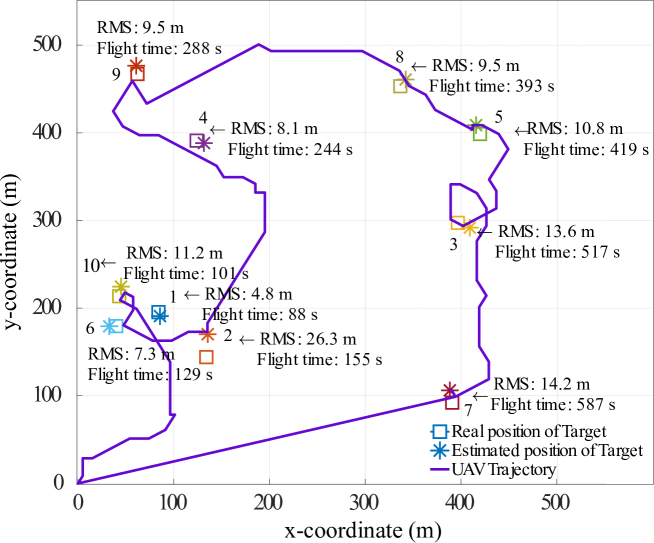
Figure 4: Simulation results with 10 mobile targets localized using a single UAV.

5.2 Monte Carlo simulations

For this experiment, all of the Monte Carlo setup parameters were kept the same as in Sec. 5.1, except for those under investigations. In addition, to ensure that the results were not random, all of the conducted experiments were performed over 100 Monte Carlo runs. The tracking algorithm was evaluated based on the following criterion:

• Estimation Error is the absolute distance between ground truth and estimated target location $\mathcal{D}_{rms}=\sum_{j=1}^{N_{tg}}d^{j}_{rms}/N_{tg}$ with $d^{j}_{rms}=[(x^{j}_{truth}-x^{j}_{est})^{2}+(y^{j}_{truth}-y^{j}_{est})^{2}]^{1/2}$.

• Flight time (s) for UAV to localize all of the targets and this includes hovering time when the UAV waits for commands from the solver to take an action.

• UAV travel distance: the total distance traveled by the UAV to track and locate all of the targets to the required location uncertainty bound; i.e the determinant of covariance being adequately small—$N_{Th}\leq 10,000~{}\text{m}^{2N_{s}}$ .

• Computational cost: We evaluate the computational cost in terms of two components: i) execution time for the solver to execute the tracking algorithm only (called non-planning time), and ii) the execution time for the solver to select the best action—planning step—as well as complete the tracking task (called planning time).

First, our search and localization algorithms were evaluated using different $\alpha$ values for Réyni reward function in (7). Table 1 presents the Monte Carlo results for $\alpha=\{0.1,0.5,0.9999\}$. In general, the $\alpha$ value does not significantly impact the overall performance. However, applying $\alpha=0.1$ provides the best localization results in terms of estimation error and search duration. Applying $\alpha=0.5$ proposed in [Ristic and Vo, 2010, Ristic et al., 2010] results in the worst performance, it increases flight time and travel distance necessary to complete the localization task. Using $\alpha=0.9999$ (considered as using KL divergence which is a popular information gain measure) helps to save UAV travel distance while sacrificing location accuracy. One explanation for this scenario is that our noisy measurement causes the predicted posterior $p(\mathbf{x}_{k+H}|\mathbf{z}_{1:k},\mathbf{z}^{(m)}_{k+1:k+H}(\mathbf{a}))$ in (7) to be less informative due to high uncertainty. Therefore, the reward function should place more emphasis on the current posterior instead by using a small $\alpha$ value or setting $\alpha\rightarrow 1$ to completely ignore the future posterior. This also explains the reason for the worst localization performance observed when $\alpha=0.5$ (equally weighting the current and the future posterior).

Table 1: Localization performance for different alpha values.

	$\alpha=0.1$	$\alpha=0.5$	$\alpha=0.9999$
RMS (m)	12.35	12.77	12.96
Flight time (s)	724	741	727
UAV travel distance (km)	2.38	2.41	2.34

Second, we conducted experiments to understand how the number of actions $N_{\mathcal{A},s}$ created by Alg. 1 affects our tracking performance in term of planning time and localization error. Table 2 shows Monte Carlo results for $N_{\mathcal{A},s}=\{2,3,4,5,6,7\}$. Increasing the number of actions beyond four does not necessarily lead to better planning decisions because of the directionality of the antenna gain. Since the antenna gain is not omnidirectional, some actions result in changing the heading where antenna gain along the propagation path between the UAV and the target is lower; when the number of actions evaluated is increased, we encounter instances when an action leading to such a lower antenna gain, in fact, results in a higher reward. This result is a consequence of the inherent uncertainties in the models used in tracking and planning. Thus, we can see that $N_{\mathcal{A},s}=4$ provides an adequate pool of actions to yield the best localization performance in terms of estimation error, flight duration, and travel distance; a desirable result for realizing real-time planning with limited computational resources.

Table 2: Localization performance for different number of actions.

Number of actions $N_{\mathcal{A},s}$	2	3	4	5	6	7
RMS (m)	14.18	12.64	12.17	12.27	12.83	12.63
Flight time (s)	840	781	693	723	756	799
UAV travel distance (km)	2.62	2.53	2.39	2.50	2.52	2.70
Planning time (s)	1.16	1.19	1.23	1.27	1.36	1.47

Third, we want to examine the performance of our proposed algorithm under an increasing number of targets; in this study, we increase the maximum number of targets $N_{tg}$ from 1 to 10. As depicted in Fig. 5, our algorithm’s estimation error was stable and invariant to the number of targets. Moreover, it is reasonable that the flight time and the travel distance increased linearly with target numbers because it took more time and power to track more targets.

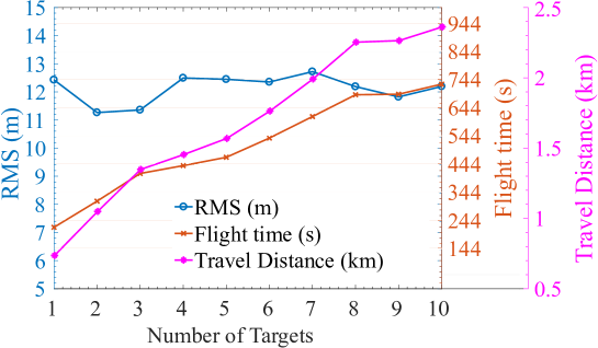
Figure 5: Localization performance for different number of targets $N_{tg}$ increase from 1 to 10.

Fourth, we examined the performance of the information gain measure, Rényi divergence, under different look-ahead horizons $H=N_{H}t_{p}$ compared to: i) Shannon entropy [Cliff et al., 2015]; ii) a naive approach that moves UAV to the closest estimated target location; and iii) a uniform search with the predefined path used in [Ristic et al., 2010]. Table 3 shows the Monte Carlo comparison results among various planning algorithms. All the parameters were reused from the Sec. 5.1, except for $\alpha=0.1$ and $N_{\mathcal{A},s}=4$ were updated based on the previous experimental results. The results demonstrated that Rényi divergence based reward function leads to significantly better planning strategies in comparison with other reward functions in terms of localization accuracy, including Shannon entropy with the same horizon settings ($N_{H}=1;t_{p}=5$). For Rényi reward function itself, the large look ahead horizon number $N_{H}>1$ helps to improve the localization accuracy; however, it requires higher computational power (planning) and causes the UAV to travel further. Using $N_{H}=1;t_{p}=5$ s provides the best trade-off between computational time and accuracy.

Table 3: Localization performance for different planning algorithms.

	Uniform	Closest Target	Shannon [Cliff et al., 2015]	Rényi
$N_{H}$	N/A	N/A	1	1	3	5	10
$t_{p}$ (s)	N/A	N/A	5	5	1	1	1
RMS (m)	18.8	13.4	12.6	12.5	12.4	12.0	11.6
Flight time (s)	921	799	774	699	889	811	822
UAV travel distance (km)	3.72	2.29	2.54	2.27	2.99	2.82	2.42
Planning Time (s)	1.58	1.11	1.38	1.28	1.53	1.65	2.71
Non-planning Time (s)	1.58	1.03	0.99	0.97	0.96	0.97	0.96

Summary: According to the above simulation results, we select $\alpha=0.1$, $N_{\mathcal{A},s}=4$, and $N_{H}=1,t_{p}=5~{}s$ as the planning parameters for the field experiment since these parameters provides the lowest computational cost, best performance in term of location estimation error, travel distance and flight time.

6 Field Experiments

We describe here our extensive experiments regime to validate our approach and evaluate the performance of our aerial robot system in the field. Our aim is to: i) investigate the possibility of signal interference from spinning motors of a UAV on RSSI measurements; ii) estimate the model parameters in the sensor model and validate the proposed model; and iii) conduct field trials to demonstrate and evaluate our system capabilities.

6.1 Rotor noise

We investigated the rotor noise to confirm that our system is not affected by the electromagnetic interference from the UAV’s motors. It also helps to clear the concern raised in [Cliff et al., 2015] that the rotor noise may affect the RSSI measurements. Four motors of the 3DR IRIS+ quad-copter shown in Fig.1 were used in this experiment. The RSSI data of a radio collar were measured across 149 MHz to 151 MHz frequency spectrum when four motors were operating at $20\%$, $50\%$, $100\%$ of its maximum speed of $10,212$ revolutions per minute. Fig 6 (a) shows the frequency spectrum of the received signal. We can see that there was no difference in the frequency characteristics when the rotors were in ON and OFF states. This result confirms that the rotors do not spin fast enough to generate high-frequency interference to impact our RSSI measurements.

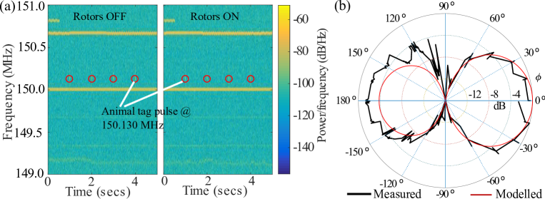
Figure 6: a) Waterfall plot for the rotor noise experiment when four motors spun at maximum rotation speed. b) Normalized antenna gain in E-plane $G(\phi)$. The red line is gain modeled pattern and black line is the normalized measured gain pattern from 30 measurements collected by rotating the UAV heading at 15^∘ intervals.

6.2 Sensor model validation and parameter estimation

Antenna Gain: The antenna gain pattern was measured to verify its directivity compared to the antenna gain model $G_{r}(\mathbf{x,u})=G_{r}(\phi)$ calculated—following [Orfanidis, 2002, p.1252]—based on the physical design as discussed in Sec. 3. Fig. 6b shows the measured and modeled radiation patterns $G_{r}(\phi)$ in the E-plane. In the measurement process, $\phi$ is evaluated as the angle between the UAV heading, changed through $0^{\circ}$ to $360^{\circ}$, and the direction from its position to a fixed location of a VHF radio tag. The result shows that the front-to-back ratio is smaller (2 dB) than expected and this is an artefact of folding the reflector on our design.

Signal propagation model parameter validation: We collected RSSI data points over a range from 10 m to 320 m between the UAV and a VHF radio tag. The tag and the UAV were kept at a height of 5 m above ground during this experiment. The tag was stationary at all times, while the UAV was directed to move away in a straight line from the tag at 10 m intervals whilst hovering at each location to allow the collection of approximately 30 measurements. The UAV heading was maintained to ensure consistent antenna gain during the experiment. Since we operated in an open terrain over a grassland, we selected the path loss exponent $n=2$ suitable for modelling free space path loss. Fig. 7 shows the measured RSSI and the propagation models obtained using a nonlinear regression algorithm to estimate model parameters; we have the following results for reference power $P_{r}^{d0}$ in (3), (4) at the reference distance $d_{0}=1$ m, and measurement noise variance $\sigma_{P}$ in (5):

• LogPath model : $P_{r}^{d0}=-15.69~{}\text{dBm}$ ; $\sigma_{P}=4.21$ dB.

• MultiPath model : $P_{r}^{d0}=-15.28~{}\text{dBm}$ ; $\sigma_{P}=2.31$ dB.

The results show that both models, as expected, derived a similar reference power $P_{r}^{d0}$ whilst providing a reasonable fit to measurement data. This affirms the validity of our propagation model. Although LogPath model is reasonable, MultiPath model is more accurate and yields a smaller measurement noise variance. The results confirm the impact of ground reflections, especially close to the signal source.

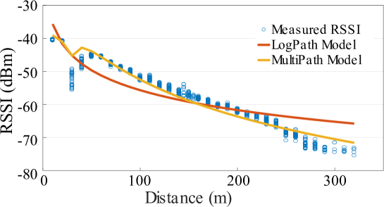
Figure 7: Plot of measured RSSI data points and its model estimates over a distance from 10 m to 320 m at 10 m intervals.

6.3 Field Trials

We designed and conducted two sets of field experiments that included 20 autonomous missions as described below.

• First set of trials (autumn season): We conducted a total of 16 autonomous flights with two mobile radio-tags to evaluate the measurement models and demonstrate the robustness of our system (see Section 6.4).

• Second set of trials (winter and wet season): We conducted 4 autonomous flights with the best performing measurement model. These experiments were aimed at demonstrating the multi-target tracking capability of our aerial robot platform under a mix of stationary (3 radio-tags) and mobile (2 radio-tags) target dynamics. In particular, we subjected our system to two highly mobile targets. Notably, these trials were conducted during the wet winter months when the test zone was over-grown with grass and shrubs. Therefore, these experiments demonstrate our system’s capability to plan a trajectory to track multiple radio-tagged objects with differing motion dynamics and under different environmental settings (see Section 6.5).

Our experiments were designed around the University of Adelaide and CASA (Civil Aviation Safety Authority, Australia) regulations governing the conduct of UAV research. Given the need to operate in an autonomous mode, our flight zone, as well as the scope of the experiment, was restricted to University-owned property designated for UAV flight tests. Prior to gaining ethical and regulatory clearances to progress our field trial to a wildlife species of interest to conservation biologists, our first objective is to evaluate and demonstrate a robust working prototype. This is a necessary condition to gain both regulatory and ethical approval. Further, it is not feasible to have a wildlife species of interest at the remote test site and conduct experiments to systematically evaluate the aerial robot system. Therefore we chose to conduct experiments with human test subjects with stipulated safety measures in an area allocated for field tests. This allowed us to create various target motion dynamics as well as obtain accurate ground truth data for tag locations to evaluate our system. Notably, our measurement model is based on the Received Signal Strength Indicator (RSSI-based) measurements of signals transmitted from radio-tags. Hence, there is no technical difference whether the radio-tags are carried by humans or wildlife.

In the field trials, the task of the aerial robot system was set to search and localize radio-tags undergoing various motion dynamics in a search area $75~{}\text{m}\times 300~{}\text{m}$ ($2.25$ hectares). Instead of wildlife, we relied on volunteers to wear a VHF radio tag of the type shown in Figure 8 on their forearm, and carry a mobile phone-based GPS data logger in their hands to obtain ground truth data. We were required to have two extra personnel stationed to maintain constant sight of the UAV as well a pilot with RePL (Remote Pilot License) in the field capable of aborting the autonomous mode and transferring control to manual operations mode.

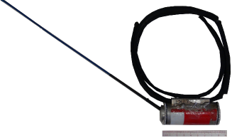
Figure 8: A collar used for radio tagging the endangered species of Southern Hairy Nose (SHN) wombats used in our field experiments. Each tag used in our experiments transmits an unmodulated on-off-keyed signal with a pulse width ranging from $10-20$ ms, at a period of approximately $1$ s, and using a unique frequency in the range of $150-152$ MHz.

6.4 First Set of Trials

In this section, we present the first set of field trials to demonstrate the planning method for tracking mobile targets. We also compare localization performance between the two signal propagation models: LogPath model and MultiPath model derived in section 6.2. We used two VHF radio collars for these trials.

Fig. 9 shows the tracking and localization results along with UAV trajectories based on the two different measurement models. As expected, we observe the UAV planning has a tendency to approach the target’s position since when the distance between the UAV and targets reduces, the RSSI measurement uncertainty is reduced. thus it helps to reduce the uncertainty and increase the information gain. We can observe a clear difference in the LogPath model and MultiPath model where UAV pursues the second target after completing the tracking task for target 1. The more accurate MultiPath model is able to track and localize the second target without needing a close approach. We can also observe that using LogPath model, where multipath propagation is not modeled but is clearly dominant close to the target, leads to a poorer localization accuracy despite the path planning algorithm leading the UAV close to the target.

Fig. 10 shows the particle distribution after the first observation is updated and when the targets are tracked and localized using the two measurement models. We can see that the solver is able to estimate the two tag positions quiet accurately even after the update using the initial observation; however, the uncertainty (as noted by the particle distribution) is still very high. Interestingly, MultiPath model location uncertainty is significantly less where target 1 is placed in the bottom half of the field while target 2 is placed in the top half of the field. Target 1, being closer to the UAV, is localized first, with under $55$ measurements for both measurement models. At the time when target 1 is localized, the uncertainty of target 2 is relatively higher for the LogPath model. The MultiPath model required significantly fewer measurements to track and localize target  2. As expected, both measurement models required significantly more measurements to localize the second target given the high measurement uncertainty associated with being much further than the first target from the UAV during its flight. Furthermore, random walk of the second target provided a challenging scenario since target 2 typically moved a larger distance around the field compared to the random walk performed by target 1.

Although the solver guides the UAV to move toward a target’s position in both measurement models, as expected, the standard LogPath model is less accurate compared to the MultiPath model shown in Fig. 7; thus, the uncertainty when using the LogPath model is higher and leads to longer time duration to localize the two tags. Albeit model uncertainty, the LogPath model is still capable of locating both moving targets within the flight time capability of the UAV. The consequence of model uncertainty resulting from the LogPath model is more apparent when the UAV makes an approach to the target and the distance to the target is less than $50$ m. This is evident in comparing the belief density in Fig. 10a at $k=125$ to that in Fig. 10b at $k=109$. We can see that the target location uncertainty increase for the LogPath model in the vicinity of 50 m and as a result, the UAV requires an increased number of maneuvers to track and locate the target.

Table 4 presents the summary comparison results of location estimates between the two measurement models. Smaller RMS (root mean square) estimation error values suggest a higher accuracy, while shorter flight times and travel distance to localize all targets are highly desirable for a practicable system given the power constrained nature of commodity UAVs. The results confirm that the MultiPath model is superior to the standard LogPath model since it has been able to account for ground reflections. Further, the UAV is not required to approach the target closely to reduce its measurement uncertainty when using the MultiPath model.

The results in Table 4 also demonstrate that our proposed method can localize two mobile targets with a shorter flight time and better accuracy compared to the method in [Cliff et al., 2015]. The RMS flight time realized with the MultiPath model is one-sixth of that in [Cliff et al., 2015]). Although our experiments were not performed with a live target animal species of interest to conservation biologists, we search and locate two mobile radio-tagged targets. In contrast, [Cliff et al., 2015] method was formulated and implemented to locate a single stationary target. However, the approach in [Cliff et al., 2015] was evaluated with a stationary radio-collared live bird while our field experiments were conducted with human test subjects.

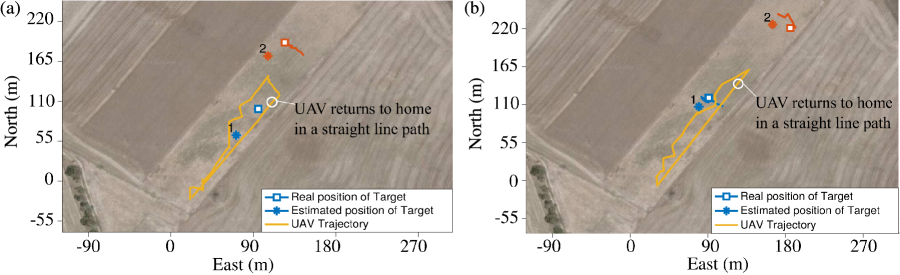
Figure 9: Field experiment results to search, track and localize two mobile tags for the two different measurement models. a) Standard LogPath. b) MultiPath.

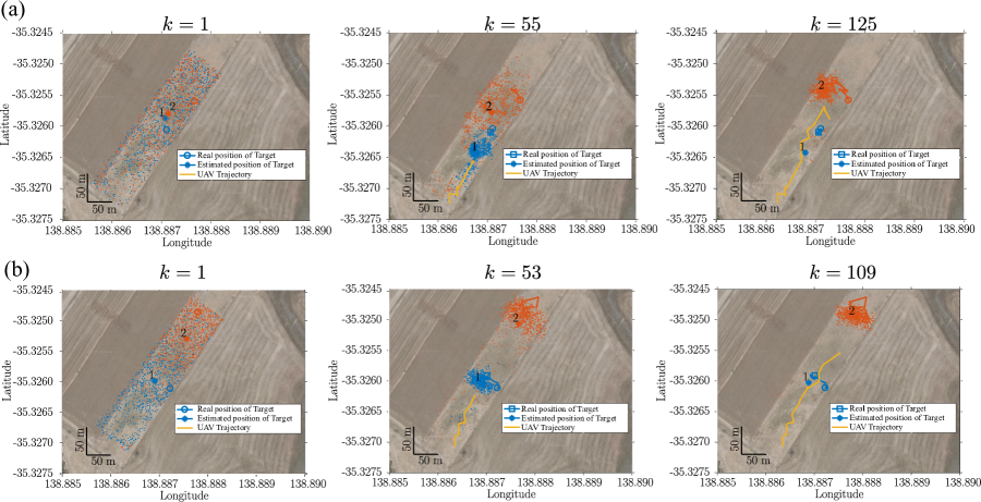
Figure 10: The intermediate distributions of belief density representing the location of the radio-tags for the two scenarios in Fig. 9. Here, Fig 10a demonstrates the convergence of the belief density of the radio-tag positions using the standard LogPath measurement model in Fig. 9a) after first observation ($k=1$), tag 1 is localized ($k=55$), and tag 2 is localized ($k=125$). Similarly, Fig 10b demonstrates the convergence of the belief density of the radio-tag positions using the MultiPath measurement model in Fig. 9b) after the first observation ($k=1$), tag 1 is localized ($k=53$), and tag 2 is localized ($k=109$). The blue and orange dots represent the starting positions of tag 1 and tag 2, respectively. The square symbols denote the ground truths of the localized tags; the star symbols denote the estimated positions of the tags. The solid yellow lines represent the UAV trajectories.

Table 4: Comparison of localization performance.

Model	Target Type	Trials	RMS (m)	Total Flight Time (s)	Travel Distance (m)
LogPath	Mobile	8	$30.1\pm 12.8$	$255\pm 104$	$549\pm 167$
MultiPath	Mobile	8	$\mathbf{22.7}\pm 13.9$	$\mathbf{138}\pm 53$	$\mathbf{286}\pm 121$
[Cliff et al., 2015]	Stationary	6	$23.8\pm 14.0$	838	N/A

6.5 Second Set of Trials

In this section, we present the second set of field trials. We use the Multipath measurement model because it provides a better measurement likelihood as shown in the tracking accuracy and flight time results in Table 4. We can see from Fig. 3, the SDR-based signal processing architecture used in our system scales to enable tracking a large number of radio tags. The number of VHF radio-tags that can be tracked and localized is only limited by the hardware, such as the battery life of the UAV and the receiver noise of the SDR. In order to demonstrate scalability and robustness, we used five radio-tags. In order to demonstrate the capability of our system to accommodate different animal behaviors, we used two highly mobile targets (target $1,2$) and three stationary targets (target $3,4,5$). Further, to demonstrate the robustness of our measurement model, we conducted these trials in the wet, winter season in South Australia where the test site was representative of a grassland with shrubs and moisture. We conducted four field missions in which the task of our aerial robot system was to track and localizes five targets as opposed to two mobile targets investigated in Section 6.4. All other experimental settings were as described in Section .6.4.

Fig. 11 depicts the UAV and mobile target trajectories together with tracking and localization results. Table. 5 presents a quantitative summary of the results from the four field missions. The results show that when the targets are highly mobile, such as target $1$ in Fig. 11a or target $1$ and $2$ in Fig. 11d, the UAV takes longer flight paths to be able to localize these highly mobile targets. This is because the UAV undertakes control actions to position itself to reduce measurement uncertainty. Consequently, we also see that the UAV path planning algorithm undertakes control actions to navigate the UAV closer or follow targets to quickly reduce measurement uncertainty. In contrast, when the targets are less mobile as shown in Fig. 11b-c, the UAV can easily localize the targets with fewer measurements, shorter flight paths, and without needing to approach the targets. Thus, when targets are less mobile, the UAV requires less flight time to accurately track and localize them. We can see that our planning for tracking approach was robust with respect to various target motion dynamics we have created. Further, the results summarized in Table 5 demonstrate that our localization results were consistently high across all four missions.

As expected, our aerial robot system can successfully track and localize multiple radio tags. In relation to the first set of field trials, we can also see that our system is: i) scalable to a larger number of VHF radio-tags; ii) robust against variations in environmental conditions; and iii) robust with respect to various target behaviors.

Table 5: Localization performance over four field missions to track and localize five radio-tagged targets.

	RMS (m)						Flight time (s)
Target dynamics	Mobile		Stationary			Mean
Target #	Target 1	Target 2	Target 3	Target 4	Target 5
Mission 1	27.3	19.1	27.2	18.1	19.9	22.3	163
Mission 2	9.3	21.8	24.9	25.4	23.7	21.0	143
Mission 3	15.0	9.3	18.7	30.6	16.3	18.0	128
Mission 4	10.0	29.6	18.4	25.1	16.6	19.9	165

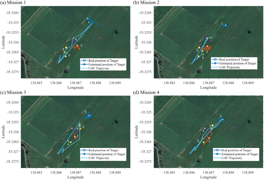
Figure 11: Four autonomous field experiment missions to search, track and localize five targets: two mobile targets (target $1,2$) and three stationary tags (target $3,4,5$). Fig. 11(a), (b), (c), and (d) corresponds to the sequence of the missions in Table 5. The square symbols denote the ground truth of the localized radio-tags; the star symbols denote the estimated positions of the radio-tags; the solid blue lines represent the trajectories planned by the autonomous aerial robot to track the set of five VHF radio-collared tags.

7 Discussion

In this section, we summarize and discuss results from our approach as well as compare and discuss our results in the context of the recent study by [Cliff et al., 2015] (see Section 7.1). We then reflect upon the lessons learned from our field trials to build, test and evaluate a new approach following a different school of thought for autonomous tracking and localization of VHF radio-tags (see Section 7.2). Our work, being a first, is not without limitations. We discuss these in Section 7.3.

7.1 Comparison

Table 6 presents a complete comparison between our proposed system and [Cliff et al., 2015] system. Notably, our search area is smaller compared to [Cliff et al., 2015] ($75~{}\text{m}\times 300~{}\text{m}$ v.s $1000~{}\text{m}\times 1000~{}\text{m}$) due to our test flight zone restrictions; however, we have set up our initial distance from the UAV home position to its farthest target’s position to be equivalent to the distance of the stationary target in [Cliff et al., 2015]; approximately 300 m. Although we have tried to replicate the distance to the location of a radio-tag, the detection range is determined by a number of factors other than the specification of the receiver and the antenna used. The detection range is heavily influenced by the transmitted power of a radio-tag, which is adjusted based on application requirements and varies in different environments, even for the radio collars form the same manufacturer. Therefore, we have not directly compared the detection range. Instead, we have tried to achieve a similar UAV-to-target distance in our experimental settings.

In general, as shown in Table 6, our system is more compact, lighter, and has a payload that is one-third of that in [Cliff et al., 2015] and consequently capable of longer flight times on any given UAV. Our total system mass being under $2$  kg enables ecologists in jurisdictions such as Australia [Civil Aviation Safety Authority, 2017], Germany [Federal Ministry of Transport and Digital Infrastructure, 2017] and India [Office Of The Director General Of Civil Aviation, 2018] to operate our system without a remote pilot license (RePL) and regulatory burdens. Moreover, as shown in Table 4, compared to the bearing-only method requiring full rotations of a UAV at each observation point, the ability to instantly collect RSSI measurements also helps reduce flight times significantly. Furthermore, as discussed in [Arulampalam et al., 2002], the computational cost for grid-based methods used in [Cliff et al., 2015] increases dramatically with the number of cells whilst the grid must be dense enough to achieve accurate estimations; e.g., a grid-based filter with $N$ cells conducts $\mathrm{O}(N^{2})$ operations per iteration, while a similar particle filter with $N$ particles only requires $\mathrm{O}(N)$ operations. Hence, the grid-based filter method is only suitable for case with stationary targets as in [Cliff et al., 2015] where the most expensive computational step, the prediction step, is skipped. Moreover, as shown in Table. 3, our planning algorithm based on Rényi divergence is superior to the Shannon entropy approach in [Cliff et al., 2015] in terms of two important metrics: i) accuracy; and ii) UAV flight time.

Table 6: Comparison between our system and [Cliff et al., 2015] system.

	Ours	[Cliff et al., 2015]
Payload (g)	260	750
Total mass (g)	1,280	2,200
Drone type	Quadcopters (smaller drone)	Octocopters (relatively larger drone)
Receiver Architecture	Software defined radio (digital-based, rapidly scan multiple frequencies to support detecting signals from multiple animals)	Analog filtering circuit and a fixed frequency narrowband receiver (analog-based, difficult to re-configure for a new frequency)
Antenna elements	Compact, lightweight, folded 2-element Yagi antenna (designed for small drone form factor)	Antenna array structure requiring a large spatial separation of two antenna elements and wire ground plane
Measurement model	Range-only (exploiting the simplicity of a range-only measurement system)	Bearing-only (antenna array, and UAV rotation at grid points with a phase difference measurement system)
Filtering method	Particle filter ($\mathrm{O}(N)$ operations per iteration)	Grid-based filter ($\mathrm{O}(N^{2})$ operations per iteration)
Planning algorithm (reward function)	Rényi divergence	Shannon entropy
Targets dynamics	Multiple mobile targets	A single stationary target
Nature of targets	Radio tags carried by humans test subjects	A radio-tagged bird (Manorina Melanocephala)

The studies in  [Dos Santos et al., 2014] and  [VonEhr et al., 2016] also used an SDR receiver and considered the problem of detecting multiple VHF radio-tag signals using a software defined radio based receiver. We can make the following observations regarding the other SDR based receiver approaches:

• The team in [Dos Santos et al., 2014] used an SDR payload on a UAV flying a pre-defined flight path to store raw signal detections. This data was post-post processed after the flight to build a signal heat map. The detection range reported in [Dos Santos et al., 2014] is $240$ m, similar to our range of $320$ m.

• This study in [VonEhr et al., 2016] discussed two software defined radio methods to collect VHF signal measurements: i) using the Doppler effect; ii) bearing measurements obtained by rotating a drone-mounted Yagi antenna, the so-called Yagi Rotation Methodology. Notably, this measurement approach is like that proposed in [Cliff et al., 2015]. Only the Yagi Rotation Methodology was implemented with a reported bearing measurement accuracy of $\pm$30 degrees. More significantly, the detection range reported in  [VonEhr et al., 2016] is up to 1.5 km. This is mainly due to a higher gain antenna (3-element Yagi vs 2-element Yagi of our system) and a more sensitive SDR, the Funcube Dongle Pro+ (FDP+) SDR used in the study. Although the Funcube Dongle Pro+ (FDP+) has a higher receiver sensitivity, it has a limited bandwidth compared the HackRF One SDR device we employed.

The mass of the sensor systems was not reported in  [VonEhr et al., 2016], but Funcube Dongle Pro+ (FDP+) SDR device with a mass of 17 g is significantly more lightweight than the HackRF One we employed with a mass of 100 g. Although detection range cannot be directly compared, we can see that together with a higher gain antenna, the hardware employed in  [VonEhr et al., 2016] achieved a significantly larger signal detection range compared with our study and the the studies in [Dos Santos et al., 2014] and [Cliff et al., 2015].

7.2 Lessons Learned

In this section, we share our observations and discuss lessons learned during our extensive set of field experiments. We also share with the research community guidelines for establishing a framework for UAV operations and related research.

We realize that the field trials are difficult for any robotics system, especially for aerial platforms where several strict regulations govern their operation. These regulations can depend on jurisdictions under which the flight operations are conducted. Typically, regulations imposed can be different depending on the purpose of the flight such as commercial or recreational and the weight class of the UAV. Currently, there is a lack of harmonization in these regulations. For instance, the requirement for a remote pilot license (RePL) applies to countries such as Australia, Germany, and India only for UAVs over 2 kg  [Civil Aviation Safety Authority, 2017, Federal Ministry of Transport and Digital Infrastructure, 2017, Office Of The Director General Of Civil Aviation, 2018]. In contrast, New Zealand and Finland only require a license for UAVs over 25 kg [Civil Aviation Authority Of New Zealand, 2015, Finnish Transport Safety Agency, 2016]. Therefore the research team must first familiarize themselves with existing regulations governing the operation of UAVs. Second, the research team needs to negotiate with the insuring body under which they operate to allow the conduct of drone-based flights as this should not be assumed. Insurance agencies can place further restrictions upon the possible field trials that can be conducted due to legal and risk issues. Dealing with these critical issues first will allow getting a framework under which to operate UAV related research such as our work in this article. At the time of doing this research, such a framework was pioneered at our University. This included the creation of a Chief Remote Pilot position and a Maintenance Controller Position. Subsequently, applying to CASA (Civil and Aviation Services, Australia) to obtain a Remotely Piloted Aircraft Operator’s Certificate (ReOC) to conduct UAV missions. The Chief Remote Pilot registered with CASA then has the authority to evaluate, manage and approve all UAV flights conducted by University staff and students.

We observed, in both field experiments and simulations, that flying the robot platform higher allows obtaining a better signal compared to ground-based systems. This is because the signal propagating to the UAV system entering an open airspace will be less attenuated than a signal propagating to a ground-based antenna and receiver system. This is since a signal propagating to a ground-based receiver will be more attenuated from potentially multiple radio wave scatters, reflectors, absorbers such as shrubs and grass in the intervening paths. Therefore, flying the robot at a higher altitude can increase the detection range. Notably, in practice, this height advantage is sometimes obtained by using lightweight aircraft and this is an expensive proposition.

The detection range of our current system is not comparable to handheld systems. However, we can see that to develop a mature tool that can function independently and survey a large area of land, we need a longer signal detection range. One simple approach to increase the range is to employ a preamplifier stage for the SDR we have used. An alternative approach is to consider an SDR device with greater sensitivity in the VHF band. For example, an earlier SDR based design  [VonEhr et al., 2016] has achieved a 1.5 km detection range. Although we could not have benefited from such a long range given the limited University allocated space for testing, the study in  [VonEhr et al., 2016] shows that a different SDR device based receiver can offer much longer detection range. Most notably, the SDR used in  [VonEhr et al., 2016] with a mass of only 17 g can be used to replace the SDR of mass 100 g we have employed to realize a further reduction in the mass of the sensor system.

The current flight time for 3DR IRIS+ quad-copter carrying our sensor system is only around 10 minutes while the detection range of the type of VHF collar we have used is around 320 m. Thus, surveying a larger area in the order of several hundred hectares is not yet feasible for our battery-equipped UAV. However, assuming we employ the SDR receiver used in  [VonEhr et al., 2016], we can achieve a reported detection range of 1.5 km. Consequently, we can see that such a detection range can achieve a survey area defined by a radius of 1.5 km to yield an area of over 700 hectares. Alternatively, if we assume that the survey area scales with the square of the detection range, we can see that an area of 225 hectares can potentially be surveyed.

Further, we observe that flying the UAV close to highly mobile targets helps to reduce localization uncertainty. We can clearly observe this in our path planning results in Fig.11a where target $1$ was running back and forth compared with the UAV trajectory for Fig.11b where target $1$ was less mobile. However, a close approach by a UAV may disturb the wildlife of interest  [Hodgson and Koh, 2016, Mulero-Pázmány et al., 2017] and can be potentially counterproductive when attempting to obtain accurate spatial and temporal information of threatened species. Wildlife reactions to a UAV differ among different species. For example, terrestrial mammals are less reactive to a UAV than birds [Mulero-Pázmány et al., 2017]. Therefore, the potential for disturbance as well as operating parameters of a UAV close to wildlife is more likely to be dependent on the species of interest. We hope to be able to address questions around appropriate operating parameters for drones in our future work. Nevertheless, we should consider maintaining a safe distance from wildlife. A practical solution can be found by flying at the highest altitude possible [Mulero-Pázmány et al., 2017]. A second approach is to use a receiver with a higher sensitivity, such as the hardware used in [Mulero-Pázmány et al., 2017], to increase the signal detection range. A third approach can be to reformulate the trajectory planning algorithm using the void probability functional proposed in [Beard et al., 2017]. Such a planning method can alter the control decisions of the path planning algorithm to avoid approaching wildlife and always maintain a safe distance.

7.3 Limitations and Future Work

While we have demonstrated a successful system, our approach is not without limitations.

Although we formulated a three-dimensional (3D) tracking problem—see equation (9)—our implementation assumed a fixed UAV altitude during the field trials. Therefore the implemented algorithm solved a two-dimensional (2D) tracking problem, that is ideally suitable for tracking and locating endangered species in largely flat terrains and grasslands. Consequently, the current approach is not suitable for tracking wildlife in hills or mountainous areas.

Notably, implementing a 3D tracking algorithm is straightforward given our formulation is already in 3D. Instead of assuming the target’s height is fixed, we need to incorporate an additional unknown variable $p^{t}_{z}$ for the target height in the target state space described by $\mathbf{x}$ in Section 3.1 and estimate the value of this unknown variable together with the 2D coordinate variables, $p^{t}_{x}$ and $p^{t}_{y}$. We have conducted simulations to evaluate a 3D formulation where the target height is unknown with an initial uncertainty ranging between $\pm 10$ m and the UAV altitude is assumed to be known exactly. The simulation results confirm that our tracking and planning algorithm is still able to track and localize multiple radio-tagged targets with unknown heights. However, the practical challenge is that we need to obtain accurate UAV altitude measurements to implement a robust 3D tracking formulation. Commercial off the shelf UAVs such as the 3DR IRIS+ that we used for building our autonomous system employs a barometer to determine height. We observed in flight tests that the height measurement is unreliable, fluctuates over time and often depends on weather conditions; as also observed in  [Szafranski et al., 2013, Liu et al., 2014]. Thus, we leave it for future work to address the problem of accurately estimating the altitude of a UAV. Two approaches that can be considered include: i) filtering the barometer sensor data using, for example, a Kalman filter [Liu et al., 2014]; and ii) the use of a LiDAR sensor or a radar-based sensor for more accurate height above ground estimations  [Schartel et al., 2018]. Alternatively, employing the existing implementation on all topographical conditions require a UAV capability to maintain a fixed relative altitude above ground.

While the software defined radio device may be replaced to achieve a greater detection range, as we discussed in Section 7.2, future work should focus on the development of new antenna designs. We designed, simulated and built a compact, folded two element Yagi antenna. Further research efforts to investigate antenna design techniques can lead to lightweight higher gain antennas to increase the detection range and survey area.

The range of the $2.4$ GHz wireless link we employed for communicating between the Ground Control System and the UAV has limited outdoor range—see Figure 2. Although, this is not a problem given the limited test site available for our work, building a practical tool requires addressing this potential problem. Thus, future work should piggyback data on the telemetry channel using the long-range $915$ MHz radio channel [VonEhr et al., 2016]. Alternatively, the Ground Control System can be removed from the loop by embedding all of the tracking and planning algorithm on the UAV itself to increase the system reliability and search area by eliminating the transmission power consumed by the additional 2.4 GHz radio channel.

Our problem formulation assumes that at least one target is visible or the UAV’s initial heading can be in the general direction of the targets. This approach is similar to that followed in [Cliff et al., 2015]. In future work, planning formulation should consider both exploration and tracking to deal with events where there are no detectable radio signals  [Charrow et al., 2015].

8 Conclusions

We have developed and demonstrated an autonomous aerial vehicle system for tracking and localizing VHF radio-tagged animals using noisy RSSI based measurements and considered the mobility of targets during their discovery in the field. The joint particle filter and POMDP with Rényi divergence based reward function provided an accurate method to explore, track and locate multiple animal collars while considering the resource constraints of the underlying UAV platform. In addition, we have realized a lightweight sensor system to minimize the payload on a UAV and achieve longer flight times.

We have demonstrated the robustness and scalability of the system in field experiments with five VHF radio collar tags under various motion dynamics. We conducted 20 autonomous flights and over 10 manual flights for sensor system evaluations. Our future goal is to evaluate our aerial robot system in field trials with different species of animals. We are in the process of obtaining ethics clearance for our first trial with the engendered Southern Hairy Nose wombats in South Australia.

Acknowledgments

This work was jointly supported by the Western Australia Parks and Wildlife (WA Parks), the Australian Research Council (LP160101177), The Shultz Foundation, the Defense Science and Technology Group (DSTG), and the University of Adelaide’s Unmanned Research Aircraft Facility. We would like to thank the support and guidance provided by Mr. Adam Kilpatrick, Chief Remote Pilot and Maintenance Controller at the University of Adelaide, for making the field trials possible and and Remote Pilot, Mr. Fei Chen, Auto-ID Lab, The University of Adelaide for support provided in conducting all of the field experiments in the study. We would like to thank conservation biologist Dr. David Taggart for helping us source the additional VHF collar radio tags as well as the support and guidance provided by Mr Keith Morris, Department of Biodiversity, Conservation and Attractions, Western Australia.

References

- Arulampalam et al., 2002 Arulampalam, M. S., Maskell, S., Gordon, N., and Clapp, T. (2002). A tutorial on particle filters for online nonlinear/non-Gaussian Bayesian tracking. IEEE Transactions on Signal Processing, 50(2):174–188.
- Bar-Shalom, 1987 Bar-Shalom, Y. (1987). Tracking and data association. Academic Press Professional, Inc.
- Beard et al., 2017 Beard, M. A., Vo, B.-T., Vo, B. N., and Arulampalam, S. (2017). Void probabilities and cauchy-schwarz divergence for generalized labeled multi-bernoulli models. IEEE Transactions on Signal Processing, 65.
- Blackman, 1986 Blackman, S. S. (1986). Multiple-target tracking with radar applications. Dedham, MA, Artech House, Inc., 1986, 463 p.
- Caballero et al., 2008 Caballero, F., Merino, L., Maza, I., and Ollero, A. (2008). A particle filtering method for wireless sensor network localization with an aerial robot beacon. In Proc. of IEEE ICRA, pages 596–601.
- Charrow et al., 2015 Charrow, B., Michael, N., and Kumar, V. (2015). Active control strategies for discovering and localizing devices with range-only sensors. In Algorithmic Foundations of Robotics XI, pages 55–71. Springer.
- Christiansen et al., 2014 Christiansen, P., Steen, K. A., Jørgensen, R. N., and Karstoft, H. (2014). Automated detection and recognition of wildlife using thermal cameras. Sensors, 14(8):13778–13793.
- Civil Aviation Authority Of New Zealand, 2015 Civil Aviation Authority Of New Zealand (2015). Advisory Circular AC101-1. [Online; accessed 1-September-2018].
- Civil Aviation Safety Authority, 2017 Civil Aviation Safety Authority (2017). AC 101-10 Remotely piloted aircraft systems - operation of excluded RPA (other than model aircraft). [Online; accessed 13-April-2018].
- Cliff et al., 2015 Cliff, O. M., Fitch, R., Sukkarieh, S., Saunders, D., and Heinsohn, R. (2015). Online Localization of Radio-Tagged Wildlife with an Autonomous Aerial Robot System. In Robotics: Science and Systems.
- Cochran and Lord Jr, 1963 Cochran, W. W. and Lord Jr, R. D. (1963). A radio-tracking system for wild animals. The Journal of Wildlife Management, pages 9–24.
- Dos Santos et al., 2014 Dos Santos, G. A. M., Barnes, Z., Lo, E., Ritoper, B., Nishizaki, L., Tejeda, X., Ke, A., Lin, H., Schurgers, C., Lin, A., et al. (2014). Small unmanned aerial vehicle system for wildlife radio collar tracking. In IEEE 11th International Conference on Mobile Ad Hoc and Sensor Systems (MASS), pages 761–766.
- Federal Ministry of Transport and Digital Infrastructure, 2017 Federal Ministry of Transport and Digital Infrastructure (2017). New rules governing drones in force. [Online; accessed 1-September-2018].
- Finnish Transport Safety Agency, 2016 Finnish Transport Safety Agency (2016). Use Of Remotely Piloted Aircraft And Model Aircraft. [Online; accessed 1-September-2018].
- Gonzalez et al., 2016 Gonzalez, L. F., Montes, G. A., Puig, E., Johnson, S., Mengersen, K., and Gaston, K. J. (2016). Unmanned Aerial Vehicles (UAVs) and artificial intelligence revolutionizing wildlife monitoring and conservation. Sensors, 16(1):97.
- Gordon et al., 1993 Gordon, N. J., Salmond, D. J., and Smith, A. F. (1993). Novel approach to nonlinear/non-Gaussian Bayesian state estimation. IEE Proceedings F - Radar and Signal Processing, 140(2):107–113.
- Hero et al., 2008 Hero, A. O., Kreucher, C. M., and Blatt, D. (2008). Information theoretic approaches to sensor management. Springer US.
- Hodgson and Koh, 2016 Hodgson, J. C. and Koh, L. P. (2016). Best practice for minimising unmanned aerial vehicle disturbance to wildlife in biological field research. Current Biology, 26(10):R404–R405.
- Hsu et al., 2008 Hsu, D., Lee, W. S., and Rong, N. (2008). A point-based POMDP planner for target tracking. In Proc. of IEEE ICRA, pages 2644–2650.
- Jakes, 1974 Jakes, W. C. (1974). Microwave mobile communications. Wiley, New York.
- Jensen et al., 2014 Jensen, A. M., Geller, D. K., and Chen, Y. (2014). Monte Carlo simulation analysis of tagged fish radio tracking performance by swarming unmanned aerial vehicles in fractional order potential fields. Journal of Intelligent & Robotic Systems, 74(1-2):287–307.
- Kaelbling et al., 1998 Kaelbling, L. P., Littman, M. L., and Cassandra, A. R. (1998). Planning and acting in partially observable stochastic domains. Artificial Intelligence, 101(1):99 –134.
- Kays et al., 2011 Kays, R., Tilak, S., Crofoot, M., Fountain, T., Obando, D., Ortega, A., Kuemmeth, F., Mandel, J., Swenson, G., Lambert, T., et al. (2011). Tracking animal location and activity with an automated radio telemetry system in a tropical rainforest. The Computer Journal, pages 1931–1948.
- Kenward, 2000 Kenward, R. E. (2000). A manual for wildlife radio tagging. Academic Press.
- Körner et al., 2010 Körner, F., Speck, R., Göktogan, A. H., and Sukkarieh, S. (2010). Autonomous airborne wildlife tracking using radio signal strength. In Proc. of IEEE/RSJ IROS, pages 107–112.
- Liu et al., 2014 Liu, H., Liu, M., Wei, X., Song, Q., Ge, Y., and Wang, F. (2014). Auto altitude holding of quadrotor UAVs with Kalman filter based vertical velocity estimation. In 11th World Congress on Intelligent Control and Automation (WCICA), pages 4765–4770.
- Mahler, 2007a Mahler, R. (2007a). PHD filters of higher order in target number. IEEE Transactions on Aerospace and Electronic Systems, 43(4).
- Mahler, 2003 Mahler, R. P. (2003). Multitarget Bayes filtering via first-order multitarget moments. IEEE Transactions on Aerospace and Electronic systems, 39(4):1152–1178.
- Mahler, 2007b Mahler, R. P. (2007b). Statistical Multisource-Multitarget Inf. Fusion. Artech House, Inc.
- Mulero-Pázmány et al., 2017 Mulero-Pázmány, M., Jenni-Eiermann, S., Strebel, N., Sattler, T., Negro, J. J., and Tablado, Z. (2017). Unmanned aircraft systems as a new source of disturbance for wildlife: A systematic review. PloS one, 12(6):e0178448.
- Office Of The Director General Of Civil Aviation, 2018 Office Of The Director General Of Civil Aviation (2018). Requirements for Operation of Civil Remotely Piloted Aircraft System (RPAS) . [Online; accessed 1-September-2018].
- Olivares-Mendez et al., 2015 Olivares-Mendez, M. A., Fu, C., Ludivig, P., Bissyandé, T. F., Kannan, S., Zurad, M., Annaiyan, A., Voos, H., and Campoy, P. (2015). Towards an autonomous vision-based unmanned aerial system against wildlife poachers. Sensors, 15(12):31362–31391.
- Orfanidis, 2002 Orfanidis, S. J. (2002). Electromagnetic waves and antennas. Rutgers University New Brunswick, NJ.
- Ossmann, 2015 Ossmann, M. (2015). Software Defined Radio with HackRF.
- Patwari et al., 2005 Patwari, N., Ash, J. N., Kyperountas, S., Hero, A. O., Moses, R. L., and Correal, N. S. (2005). Locating the nodes: cooperative localization in wireless sensor networks. IEEE Signal processing magazine, 22(4):54–69.
- Posch and Sukkarieh, 2009 Posch, A. and Sukkarieh, S. (2009). UAV based search for a radio tagged animal using particle filters. In Australasian Conference on Robotics and Automation (ACRA), Sydney, Australia, Dec, pages 2–4.
- Reuter et al., 2014 Reuter, S., Vo, B.-T., Vo, B.-N., and Dietmayer, K. (2014). The labeled multi-Bernoulli filter. IEEE Transactions on Signal Processing, 62(12):3246–3260.
- Ristic, 2013 Ristic, B. (2013). Particle Filters for Random Set Models. Springer-Verlag New York.
- Ristic et al., 2004 Ristic, B., Arulampalam, S., and Gordon, N. c. (2004). Beyond the Kalman filter : particle filters for tracking applications. Artech House.
- Ristic et al., 2010 Ristic, B., Morelande, M., and Gunatilaka, A. (2010). Information driven search for point sources of gamma radiation. Signal Processing, 90(4):1225–1239.
- Ristic and Vo, 2010 Ristic, B. and Vo, B.-N. (2010). Sensor control for multi-object state-space estimation using random finite sets . Automatica, 46(11):1812 – 1818.
- Särkkä et al., 2014 Särkkä, S., Viikari, V., and Jaakkola, K. (2014). RFID-based butterfly location sensing system. In European Signal Processing Conference (EUSIPCO), pages 2045–2049.
- Schartel et al., 2018 Schartel, M., Burr, R., Schoeder, P., Rossi, G., Hügler, P., Mayer, W., and Waldschmidt, C. (2018). Radar-based altitude over ground estimation of UAVs. In 11th German Microwave Conference (GeMiC), pages 103–106.
- Selby et al., 2011 Selby, W., Corke, P., and Rus, D. (2011). Autonomous aerial navigation and tracking of marine animals. In Proc. of the Australian Conference on Robotics and Automation (ACRA).
- Silver and Veness, 2010 Silver, D. and Veness, J. (2010). Monte-Carlo planning in large POMDPs. In Advances in neural information processing systems, pages 2164–2172.
- Stone et al., 2013 Stone, L. D., Streit, R. L., Corwin, T. L., and Bell, K. L. (2013). Bayesian multiple target tracking. Artech House.
- Streit and Luginbuhl, 1994 Streit, R. L. and Luginbuhl, T. E. (1994). Maximum likelihood method for probabilistic multihypothesis tracking. In Signal and Data Processing of Small Targets 1994, volume 2235, pages 394–406. International Society for Optics and Photonics.
- Szafranski et al., 2013 Szafranski, G., Czyba, R., Janusz, W., and Blotnicki, W. (2013). Altitude estimation for the UAV’s applications based on sensors fusion algorithm. In 2013 International Conference on Unmanned Aircraft Systems (ICUAS), pages 508–515.
- Thomas et al., 2012 Thomas, B., Holland, J. D., and Minot, E. O. (2012). Wildlife tracking technology options and cost considerations. Wildlife Research, 38(8):653–663.
- Tokekar et al., 2010 Tokekar, P., Bhadauria, D., Studenski, A., and Isler, V. (2010). A robotic system for monitoring carp in Minnesota lakes. Journal of Field Robotics, 27(6):779–789.
- Tremblay et al., 2017 Tremblay, J. A., Desrochers, A., Aubry, Y., Pace, P., and Bird, D. M. (2017). A low-cost technique for radio-tracking wildlife using a small standard unmanned aerial vehicle. Journal of Unmanned Vehicle Systems, 5(3):102–108.
- Vander Hook et al., 2014 Vander Hook, J., Tokekar, P., and Isler, V. (2014). Cautious Greedy Strategy for Bearing-only Active Localization: Analysis and Field Experiments. Journal of Field Robotics, 31(2):296–318.
- Vo and Ma, 2006 Vo, B.-N. and Ma, W.-K. (2006). The Gaussian mixture probability hypothesis density filter. IEEE Transactions on signal processing, 54(11):4091.
- Vo et al., 2014 Vo, B.-N., Vo, B.-T., and Phung, D. (2014). Labeled random finite sets and the Bayes multi-target tracking filter. IEEE Transactions on Signal Processing, 62(24):6554–6567.
- Vo and Vo, 2013 Vo, B.-T. and Vo, B.-N. (2013). Labeled random finite sets and multi-object conjugate priors. IEEE Transactions on Signal Processing, 61(13):3460–3475.
- Vo et al., 2009 Vo, B.-T., Vo, B.-N., and Cantoni, A. (2009). The cardinality balanced multi-target multi-Bernoulli filter and its implementations. IEEE Transactions on Signal Processing, 57(2):409–423.
- VonEhr et al., 2016 VonEhr, K., Hilaski, S., Dunne, B. E., and Ward, J. (2016). Software Defined Radio for direction-finding in UAV wildlife tracking. In IEEE International Conference on Electro Information Technology (EIT), pages 0464–0469.
- Ward et al., 2016 Ward, S., Hensler, J., Alsalam, B., and Gonzalez, L. F. (2016). Autonomous UAVs wildlife detection using thermal imaging, predictive navigation and computer vision. In Proceedings of the IEEE Aerospace Conference, pages 1–8.
- Webber et al., 2017 Webber, D., Hui, N., Kastner, R., and Schurgers, C. (2017). Radio receiver design for Unmanned Aerial wildlife tracking. In International Conference on Computing, Networking and Communications (ICNC),, pages 942–946.
- Wikelski et al., 2007 Wikelski, M., s, R. W., Kasdin, N. J., Thorup, K., Smith, J. A., and Swenson, G. W. (2007). Going wild: what a global small-animal tracking system could do for experimental biologists. Journal of Experimental Biology, 210(2):181–186.
- Zhou, 2013 Zhou, D. (2013). Thermal image-based deer detection to reduce accidents due to deer-vehicle collisions.