Approximating the Sum of Independent Non-Identical Binomial Random Variables

Abstract

The distribution of sum of independent non-identical binomial random variables is frequently encountered in areas such as genomics, healthcare, and operations research. Analytical solutions to the density and distribution are usually cumbersome to find and difficult to compute. Several methods have been developed to approximate the distribution, and among these is the saddlepoint approximation. However, implementation of the saddlepoint approximation is non-trivial and, to our knowledge, an R package is still lacking. In this paper, we implemented the saddlepoint approximation in the sinib package. We provide two examples to illustrate its usage. One example uses simulated data while the other uses real-world healthcare data. The sinib package addresses the gap between the theory and the implementation of approximating the sum of independent non-identical binomials.

1 Introduction

Convolution of independent non-identical binomial random variables appears in a variety of applications, such as analysis of variant-region overlap in genomics [1], calculation of bundle compliance statistics in healthcare organizations [2], and reliability analysis in operations research [3].

Computating the exact distribution of the sum of non-identical independent binomial random variables requires enumeration of all possible combinations of binomial outcomes that satisfy the totality constraint. However, analytical solutions are often difficult to find for sums of greater than two binomial random variables. Several studies have proposed approximate solutions [4, 5]. In particular, Eisinga et al. examined the saddlepoint approximation, and compared them to exact solutions [6]. They note that, in practice, these approximations are often as good as the exact solution and are easy to implement in most statistical software.

Despite the theoretical development of aforementioned approximate solutions, a software implementation in R is still lacking. The stats package includes functions for the most frequently used distribution such as dbinom and dnorm. In addition, it also include less frequent distributions such as pbirthday. However, it does not contain functions for distribution of sum of independent non-identical binomials. Another package, EQL, provides a saddlepoint function to approximate the mean of i.i.d random variables. However, this function does not apply to the case where the random variables are not identical. In this paper, we address this deficiency by implementing a saddlepoint approximation in the open source package sinib (sum of independent non-identical binomial random variables). The package provides the standard suite of probability (psinib, distribution (dsinib, quantile (qsinib, and random number generator (rsinib functions. The package is accompanied by a detailed documentation, and can be easily integrated into existing applications.

The remainder of this paper is organized as follows, section 2 formulates the distribution of sum of independent non-identical binomial random variables. Section 3 gives an overview of the saddlepoint approximation. Section 4 describes the design and implementation of the sinib package. Section 5 uses two examples to illustrate its usage. As a bonus, we assess the accuracty of saddlepoint approximation in both examples. Section 6 draws final conclusion and discusses possible future development of the package.

2 Overview of the distribution

Suppose $X_{1}$,…,$X_{m}$ are independent non-identical binomial random variables, and $S_{m}=\sum_{i=1}^{m}X_{i}$. We are interested in finding the distribution of $S_{m}$.

$$P(S_{m}=s)=P(X_{1}+X_{2}+...+X_{m}=s)$$ (1)

In the special case of $m=2$, the probability simplifies to

$$P(S_{2}=s)=P(X_{1}+X_{2}=s)=\sum_{i=0}^{s}P(X_{1}=i)P(X_{2}=s-i)$$ (2)

Computation of the exact distribution often involves enumerating all possible combinations of each variable that sums to a given value, which becomes infeasible when n is large. A fast recursion method to compute the exact distribution has been proposed [7, 8]. The algorithm is as follows:

1. Compute the exact distribution of each $X_{i}$.

2. Calculate the distribution of $S_{2}=X_{1}+X_{2}$ using equation 2 and cache the result.

3. Calculate $S_{r}=S_{r-1}+X_{i}$ for $r=3,4,...,m$.

Although the recursion speeds up the calculation, studies have shown that the result may be numerically unstable due to round-off error in computing $P(S_{r}=0)$ if r is large[9, 6]. Therefore, approximation methods are still widely used in literature.

3 Saddlepoint approximation

The saddlepoint approximation, first proposed by [10] and later extended by [11], provides highly accurate approximations for the probability and density of any distribution. In brief, let $M(u)$ be the moment generating function, and $K(u)=\log(M(u))$ be the cumulant generating function. The saddlepoint approximation to the PDF of the distribution is given as:

$$\hat{P}_{1}(S=s)=\frac{\exp(K(\hat{u})-\hat{u}s)}{\sqrt{2\pi K^{\prime\prime}(\hat{u})}}$$ (3)

where $\hat{u}$ is the unique value that satisfies $K^{\prime}(\hat{u})=s$.

[6] applied the saddlepoint approximation to sum of independent non-identical binomial random variables. Suppose that $X_{i}\sim Binomial(n_{i},p_{i})\text{ for }i=1,2,...,m$. The cumulant generating function of $S_{m}=\sum_{i=1}^{m}X_{i}$ is:

$$K(u)=\sum_{i=1}^{m}n_{i}\ln(1-p_{i}+p_{i}\exp(u))$$ (4)

The first- and second-order derivative of $K(u)$ are:

$$K^{\prime}(u)=\sum_{i=1}^{m}n_{i}q_{i}$$ (5)

$$K^{\prime\prime}(u)=\sum_{i=1}^{m}n_{i}q_{i}(1-q_{i})$$ (6)

where $q_{i}=p_{i}exp(u)(1-p_{i}+p_{i}\exp(u))$.

The saddlepoint of $\hat{u}$ can be obtained by solving $K^{\prime}(\hat{u})=s$. A unique root can always be found because $K(u)$ is strictly convex and therefore $K^{\prime}(u)$ is monotonically increasing on the real line.

The above shows the first-order approximation of the distribution. The approximation can be improved by adding a second-order correction term [12].

$$\hat{P}_{2}(S=s)=\hat{P}_{1}(S=s)\Big{\{}1+\frac{K^{\prime\prime\prime\prime}(\hat{u})}{8[K^{\prime\prime}(\hat{u})]^{2}}-\frac{5[K^{\prime\prime\prime}(\hat{u})]^{2}}{24[K^{\prime\prime}(\hat{u})]^{3}}\Big{\}}$$ (7)

where

$$K^{\prime\prime\prime}(\hat{u})=\sum_{i=1}^{m}n_{i}q_{i}(1-q_{i})(1-2q_{i})$$

and

$$K^{\prime\prime\prime\prime}(\hat{u})=\sum_{i=1}^{m}n_{i}q_{i}(1-q_{i})[1-6q_{i}(1-q_{i})]$$

Although the saddlepoint equation cannot be solved at boundaries $s=0$ and $s=\sum_{i=1}^{m}n_{i}$, their exact probabilities can be computed easily:

$$P(S=0)=\prod_{i=1}^{m}(1-p_{i})^{n_{i}}$$ (8)

$$P(S=\sum_{i=1}^{m}n_{i})=\prod_{i=1}^{m}p_{i}^{n_{i}}$$ (9)

Incorporation of boundary solutions into the approximation gives:

$$\bar{P}(S=s)=\begin{cases}P(S=0),&s=0\\ [1-P(S=0)-P(S=\sum_{i=1}^{m}n_{i})]\frac{\hat{P}_{2}(S=s)}{\sum_{i=1}^{\sum_{i=1}^{m}n_{i}-1}\hat{P}_{2}(S=i)},&0<s<\sum_{i=1}^{m}n_{i}\\ P(S=\sum_{i=1}^{m}n_{i}),&s=\sum_{i=1}^{m}n_{i}\end{cases}$$ (10)

We implemented equation 10 as the final approxmation of the probability density function. For the cumulative density, [12] gave the following approximator:

$$\hat{P}_{3}(S\geq s)=\begin{cases}1-\Phi(\hat{w})-\phi(\hat{w})(\frac{1}{\hat{w}}-\frac{1}{\hat{u_{1}}}),&\text{if }s\neq E(S)\text{ and }\hat{u}\neq 0\\ \frac{1}{2}-\frac{1}{\sqrt{2\pi}}\big{[}\frac{K^{\prime\prime\prime}(0)}{6K^{\prime\prime}(0)^{3/2}}-\frac{1}{2\sqrt{K^{\prime\prime}(0)}}\big{]},&\text{otherwise}\end{cases}$$ (11)

where $\hat{w}=\text{sign}(\hat{u})[2\hat{u}K^{\prime}(\hat{u})-2K(\hat{u})]^{1/2}$ and $\hat{u}_{1}=[1-\exp(-\hat{u})][K^{\prime\prime}(\hat{u})]^{1/2}$. The letters $\Phi$ and $\phi$ denotes the probability and density of the standard normal distribution.

The accuracy can be improved by adding a second-order continuity correction:

$$\hat{P}_{4}(S\geq s)=\hat{P}_{3}(S\geq s)-\phi(\hat{w})\Big{[}\frac{1}{\hat{u}_{2}}\Big{(}\frac{\hat{\kappa}_{4}}{8}-\frac{5\hat{\kappa}^{2}_{3}}{24}\Big{)}-\frac{1}{\hat{u}_{2}^{3}}-\frac{\hat{\kappa}_{3}}{2\hat{u}_{2}^{2}}+\frac{1}{\hat{w}^{3}}\Big{]}$$ (12)

where $\hat{u}_{2}=\hat{u}[K^{\prime\prime}(\hat{u})]^{1/2}$, $\hat{\kappa}_{3}=K^{\prime\prime\prime}(\hat{u})[K^{\prime\prime}(\hat{u})]^{-3/2}$, and $\hat{\kappa}_{4}=K^{\prime\prime\prime\prime}(\hat{u})[K^{\prime\prime}(\hat{u})]^{-2}$.

We implemented equation 12 in the package to approximate the cumulative distribution.

4 The sinib package

The package used only functions in base R and the stats package to minimize compatibility issues. The arguments for the functions in the sinib package are designed to have similar meaning to those in the stats package, thereby minimizing the learning required. To illustrate, we compare the arguments of the *binom and the *sinib functions.

From the help page of the binomial distribution:

• x, q: vector of quantiles.

• p: vector of probabilities.

• n: number of observations.

• size: number of trials.

• prob: probability of success on each trial.

• log, log.p: logical; if TRUE, probabilities p are given as log(p).

• lower.tail: logical; if TRUE (default), probabilities are $P[X\leq x]$, otherwise, $P[X>x]$.

Since the distribution of sum of independent non-identical binomials is defined by a vector of trial and probability pairs (each pair for one constituent binomial), it was neccessary to redefine these arguments in the *sinib functions. Therefore, the following two arguments need to be redefined:

• size: integer vector of number of trials.

• prob: numeric vector of success probabilities.

All other arguments remain the same. It is worth noting that when size and prob arguments are given as vectors of length 1, the *sinib functions redues to *binom functions:

# Binomial:dbinom(x = 1, size = 2, prob = 0.5)[1] 0.5# Sum of binomials:library(sinib)dsinib(x = 1, size = 2, prob = 0.5)[1] 0.5

With that in mind, the next section shows a few examples to illustrate the usage of sinib.

5 Two examples

5.1 Sum of two binomials

We use two examples to illustrate the use of this package, starting from the simplest case of two binomial random variables with the same mean but different sizes, $X\sim Bin(n,p)$ and $Y\sim Bin(m,p)$. The distribution of $S=X+Y$ has an analytical solution, $S\sim Bin(m+n,p)$. We can therefore use different combinations of $(m,n,p)$ to assess the accuracy of the saddlepoint approximation of the CDF. We use $m,n=\{10,100,1000\}$ and $p=\{0.1,0.5,0.9\}$ to assess the approximation. The ranges of m and n are chosen to be large and the value of p are chosen to represent both boundaries.

library(foreach)library(data.table)library(cowplot)library(sinib)# Comparison of CDF between truth and approximation:data=foreach(m=c(10,100,1000),.combine=’rbind’)%do%{foreach(n=c(10,100,1000),.combine=’rbind’)%do%{foreach(p=c(0.1, 0.5, 0.9),.combine=’rbind’)%do%{a=pbinom(q=0:(m+n),size=(m+n),prob = p)b=psinib(q=0:(m+n),size=as.integer(c(m,n)),prob=c(p,p))data.table(s=seq_along(a),truth=a,approx=b,m=m,n=n,p=p)}}}ggplot(data,aes(x=truth,y=approx,color=as.character(p)))+geom_point(alpha=0.5)+facet_grid(m~n)+theme_bw()+scale_color_discrete(name=’prob’)+xlab(’Truth’)+ylab(’Approximation’)

Figure 1: Comparison of CDF between truth and approximation

Figure 1 shows that the approximations are close to the ground truths across a range of parameters. We can further examine the accuracy by looking at the differences between the approximations and the ground truths.

p2=ggplot(data[m==100&n==100],aes(x=s,y=truth-approx,color=as.character(p)))+geom_point(alpha=0.5)+theme_bw()+scale_color_discrete(name=’prob’)+xlab(’Quantile’)+ylab(’Truth-Approximation’)+geom_vline(xintercept=200*0.5,color=’green’,linetype=’longdash’)+geom_vline(xintercept=200*0.1,color=’red’,linetype=’longdash’)+geom_vline(xintercept=200*0.9,color=’blue’,linetype=’longdash’)

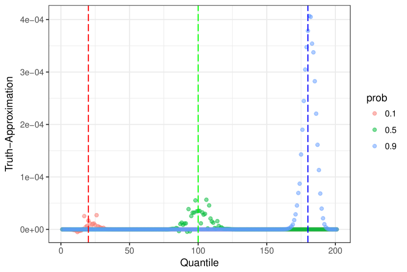
Figure 2: Difference in CDF between the ground truth and the approximation

Figure 2 shows the difference between the truth and the approximation for $m=n=100$. The dashed line indicate the mean of each random variable. The approximations perform well overall. The largest difference occurs around the mean (dashed lines), but the largest deviation is less than 5e-4. We can also examine the approximation for the PDF.

# Comparison of PDF between truth and approximation:data=foreach(m=c(10,100,1000),.combine=’rbind’)%do%{foreach(n=c(10,100,1000),.combine=’rbind’)%do%{foreach(p=c(0.1, 0.5, 0.9),.combine=’rbind’)%do%{a=dbinom(x=0:(m+n),size=(m+n),prob = p)b=dsinib(x=0:(m+n),size=as.integer(c(m,n)),prob=c(p,p))data.table(s=seq_along(a),truth=a,approx=b,m=m,n=n,p=p)}}}ggplot(data,aes(x=truth,y=approx,color=as.character(p)))+geom_point(alpha=0.5)+facet_grid(m~n)+theme_bw()+scale_color_discrete(name=’prob’)+xlab(’Truth’)+ylab(’Approximation’)

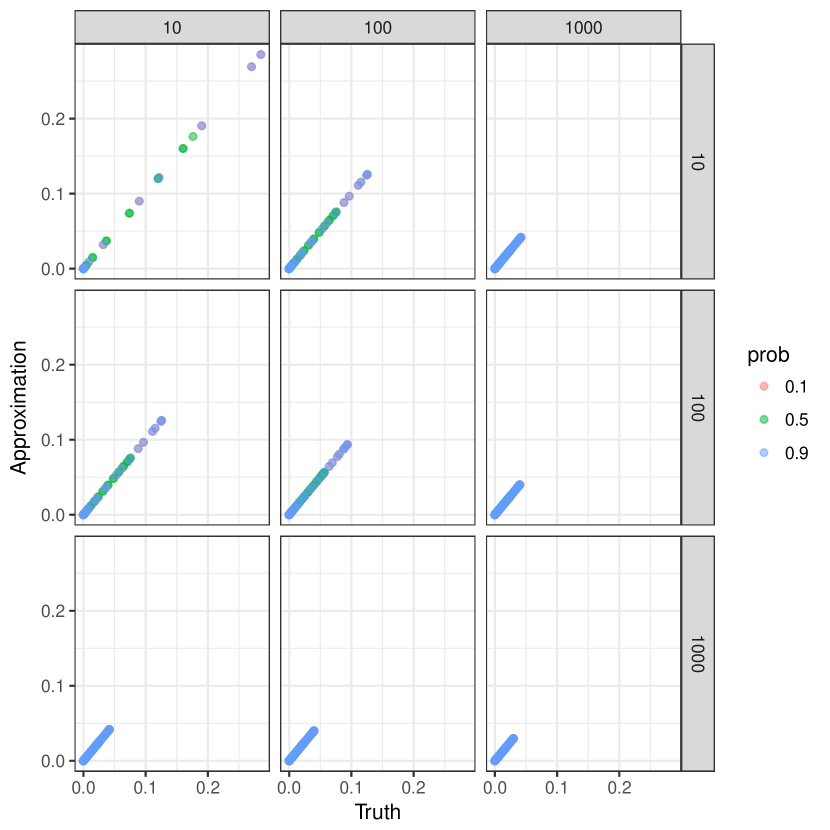
Figure 3: Comparison of PDF between truth and approximation

Figure 3 shows that the approximations and the ground truths are similar. Once again, we examine the difference between the truth and the approximation. One example for $m=n=100$ is shown in figure 4. As before, the approximation degrades around the mean, but the largest deviation is less than 4e-7.

p4=ggplot(data[m==100&n==100],aes(x=s,y=truth-approx,color=as.character(p)))+geom_point(alpha=0.5)+theme_bw()+scale_color_discrete(name=’prob’)+xlab(’Quantile’)+ylab(’Truth-Approximation’)+geom_vline(xintercept=200*0.5,color=’green’,linetype=’longdash’)+geom_vline(xintercept=200*0.1,color=’red’,linetype=’longdash’)+geom_vline(xintercept=200*0.9,color=’blue’,linetype=’longdash’)

Figure 4: Difference in PDF between truth and approximation

5.2 Healthcare monitoring

In the second example, we used a health system monitoring dataset by [2]. Suppose $n_{i}$ and $p_{i}$ take the following values.

size=as.integer(c(12, 14, 4, 2, 20, 17, 11, 1, 8, 11))prob=c(0.074, 0.039, 0.095, 0.039, 0.053, 0.043, 0.067, 0.018, 0.099, 0.045)

Since it is difficult to find an analytical solution to the density, we estimated the density with simulation (1e8 trials) and treated it as the ground truth. We then compared simulations with 1e3, 1e4, 1e5, and 1e6 trials, as well as the saddlepoint approximation, to the ground truth.

# Sinib:approx=dsinib(0:sum(size),size,prob)approx=data.frame(s=0:sum(size),pdf=approx,type=’saddlepoint’)# Simulation:data=foreach(n_sim=10^c(3:6,8),.combine=’rbind’)%do%{n_binom=length(prob)set.seed(42)mat=matrix(rbinom(n_sim*n_binom,size,prob),nrow=n_binom,ncol=n_sim)S=colSums(mat)sim=sapply(X = 0:sum(size), FUN = function(x) {sum(S==x)/length(S)})data.table(s=0:sum(size),pdf=sim,type=n_sim)}data=rbind(data,approx)truth=data[type==’1e+08’,]merged=merge(truth[,list(s,pdf)],data,by=’s’,suffixes=c(’_truth’,’_approx’))merged=merged[type!=’1e+08’,]ggplot(merged,aes(pdf_truth,pdf_approx))+geom_point()+facet_grid(~type)+geom_abline(intercept=0,slope=1)+theme_bw()+xlab(’Truth’)+ylab(’Approx’)

Figure 5: Comparison of PDF between truth and approximation

Figure 5 shows that the simulation with 1e6 trials and the saddlepoint approximation are visually indistinguishable from the ground truth, while simulations with smaller sizes shows clear deviations from the truth. To be precise, we plotted the difference in PDF between the truth and the approximation.

merged[,diff:=pdf_truth-pdf_approx]ggplot(merged,aes(s,diff))+geom_point()+facet_grid(~type)+theme_bw()+xlab(’Quantile’)+ylab(’Truth-Approx’)

Figure 6: Comparison of PDF between truth and approximation

Figure 6 shows that that the saddlepoint method and the simulation with 1e6 both provide good approximations, while simulations of smaller sizes show clear deviations. Note that the saddlepoint approximation is 5 times faster than the simulation of 1e6 trials.

ptm=proc.time()n_binom=length(prob)mat=matrix(rbinom(n_sim*n_binom,size,prob),nrow=n_binom,ncol=n_sim)S=colSums(mat)sim=sapply(X = 0:sum(size), FUN = function(x) {sum(S==x)/length(S)})proc.time()-ptm#    user  system elapsed#   1.008   0.153   1.173ptm=proc.time()approx=dsinib(0:sum(size),size,prob)proc.time()-ptm#   user  system elapsed#  0.025   0.215   0.239

6 Conclusion and future directions

In this paper, we presented an implementation of the saddlepoint method to approximate the distribution of sum of independent and non-identical binomials. We assessed the accuracy of the method by, first, comparing it with the analytical solution on a simple case of two binomials, and second, with the simulated ground truth on a real-world dataset in healthcare monitoring. These assessments suggest that, while the saddlepoint approximation deviates from the ground truth around the means, it generally provides an approximation superior to simulation in terms of both speed and accuracy. Overall, the sinib package addresses the gap between the theory and implementation on the approximation of sum of independent and non-identical binomial random variables.

In the future, we aim to explore other approximation methods such as the Kolmogorov approximation and the Pearson curve approximation described by [7].

References

- [1] Ellen M Schmidt, Ji Zhang, Wei Zhou, Jin Chen, Karen L Mohlke, Y Eugene Chen, and Cristen J Willer. GREGOR: evaluating global enrichment of trait-associated variants in epigenomic features using a systematic, data-driven approach. Bioinformatics, 31(16):2601–2606, August 2015.
- [2] James C Benneyan and Aysun Taşeli. Exact and approximate probability distributions of evidence-based bundle composite compliance measures. Health Care Management Science, 13(3):193–209, February 2010.
- [3] Samuel Kotz and Norman L Johnson. Effects of False and Incomplete Identification of Defective Items on the Reliability of Acceptance Sampling. Operations Research, 32(3):575–583, May 1984.
- [4] Norman L Johnson, Adrienne W Kemp, and Samuel Kotz. Univariate Discrete Distributions. Johnson/Univariate Discrete Distributions. John Wiley & Sons, Inc., Hoboken, NJ, USA, January 2005.
- [5] Joel K Jolayemi. A unified approximation scheme for the convolution of independent binomial variables. Applied Mathematics and Computation, 49(2-3):269–297, June 1992.
- [6] Rob Eisinga, Manfred Te Grotenhuis, and Ben Pelzer. Saddlepoint approximations for the sum of independent non-identically distributed binomial random variables. Statistica Neerlandica, 67(2):190–201, May 2013.
- [7] Ken Butler and Michael A Stephens. The Distribution of a Sum of Independent Binomial Random Variables. Methodology and Computing in Applied Probability, 19(2):557–571, December 2016.
- [8] J Arthur Woodward and Christina G S Palmer. On the exact convolution of discrete random variables. Applied Mathematics and Computation, 83(1):69–77, April 1997.
- [9] Hong Yili. On Computing the Distribution Function for the Sum of Independent and Non-identical Random Indicators .
- [10] H E Daniels. Saddlepoint Approximations in Statistics. The Annals of Mathematical Statistics, 25(4):631–650, December 1954.
- [11] Robert Lugannani and Stephen Rice. Saddle Point Approximation for the Distribution of the Sum of Independent Random Variables. Advances in Applied Probability, 12(2):475, June 1980.
- [12] H E Daniels. Tail Probability Approximations. International Statistical Review / Revue Internationale de Statistique, 55(1):37–48, April 1987.