Linearly-Recurrent Autoencoder Networks for Learning Dynamics

Abstract

This paper describes a method for learning low-dimensional approximations of nonlinear dynamical systems, based on neural-network approximations of the underlying Koopman operator. Extended Dynamic Mode Decomposition (EDMD) provides a useful data-driven approximation of the Koopman operator for analyzing dynamical systems. This paper addresses a fundamental problem associated with EDMD: a trade-off between representational capacity of the dictionary and over-fitting due to insufficient data. A new neural network architecture combining an autoencoder with linear recurrent dynamics in the encoded state is used to learn a low-dimensional and highly informative Koopman-invariant subspace of observables. A method is also presented for balanced model reduction of over-specified EDMD systems in feature space. Nonlinear reconstruction using partially linear multi-kernel regression aims to improve reconstruction accuracy from the low-dimensional state when the data has complex but intrinsically low-dimensional structure. The techniques demonstrate the ability to identify Koopman eigenfunctions of the unforced Duffing equation, create accurate low-dimensional models of an unstable cylinder wake flow, and make short-time predictions of the chaotic Kuramoto-Sivashinsky equation.

65P99, 37M10, 37M25, 47-04, 47B33

1 Introduction

The Koopman operator first introduced in [11] describes how Hilbert space functions on the state of a dynamical system evolve in time. These functions, referred to as observables, may correspond to measurements taken during an experiment or the output of a simulation. This makes the Koopman operator a natural object to consider for data-driven analysis of dynamical systems. Such an approach is also appealing because the Koopman operator is linear, though infinite dimensional, enabling the concepts of modal analysis for linear systems to be extended to dynamics of observables in nonlinear systems. Hence, the invariant subspaces and eigenfunctions of the Koopman operator are of particular interest and provide useful features for describing the system if they can be found. For example, level sets of Koopman eigenfunctions may be used to form partitions of the phase space into ergodic sets along with periodic and wandering chains of sets [2]. They allow us to parameterize limit cycles and tori as well as their basins of attraction. The eigenvalues allow us to determine the stability of these structures and the frequencies of periodic and quasiperiodic attractors [20]. Furthermore, by projecting the full state as an observable onto the eigenfunctions of the Koopman operator, it is decomposed into a linear superposition of components called Koopman modes which each have a fixed frequency and rate of decay. Koopman modes therefore provide useful coherent structures for studying the system’s evolution and dominant pattern-forming behaviors. This has made the Koopman operator a particularly useful object of study for high-dimensional spatiotemporal systems like unsteady fluid dynamics beginning with the work of Mezić on spectral properties of dynamical systems [19] then Rowley [27] and Schmid [28] on the Dynamic Mode Decomposition (DMD) algorithm. Rowley, recognizing that DMD furnishes an approximation of the Koopman operator and its modes, applied the technique to data collected by simulating a jet in a crossflow. The Koopman modes identified salient patterns of spatially coherent structure in the flow which evolved at fixed frequencies.

The Extended Dynamic Mode Decomposition (EDMD) [33] is an algorithm for approximating the Koopman operator on a dictionary of observable functions using data. If a Koopman-invariant subspace is contained in the span of the observables included in the dictionary, then as long as enough data is used, the representation on this subspace will be exact. EDMD is a Galerkin method with a particular data-driven inner product as long as enough data is used. Specifically, this will be true as long as the rank of the data matrix is the same as the dimension of the subspace spanned by the (nonlinear) observables [25]. However, the choice of dictionary is ad hoc, and it is often not clear how to choose a dictionary that is sufficiently rich to span a useful Koopman-invariant subspace. One might then be tempted to consider a very large dictionary, with enough capacity to represent any complex-valued function on the state space to within an $\epsilon$ tolerance. However, such a dictionary has combinatorial growth with the dimension of the state space and would be enormous for even modestly high-dimensional problems.

One approach to mitigate the cost of large or even infinite dictionaries is to formulate EDMD as a kernel method referred to as KDMD [34]. However, we are still essentially left with the same problem of deciding which kernel function to use. Furthermore, if the kernel or EDMD feature space is endowed with too much representational capacity (a large dictionary), the algorithm will over-fit the data (as we shall demonstrate with a toy problem in Example 2.1). EDMD and KDMD also identify a number of eigenvalues, eigenfunctions, and modes which grows with the size of the dictionary. If we want to build reduced order models of the dynamics, a small collection of salient modes or a low-dimensional Koopman invariant subspace must be identified. It is worth mentioning two related algorithms for identifying low-rank approximations of the Koopman operator. Optimal Mode Decomposition (OMD) [35] finds the optimal orthogonal projection subspace of user-specified rank for approximating the Koopman operator. Sparsity-promoting DMD [10] is a post-processing method which identifies the optimal amplitudes of Koopman modes for reconstructing the snapshot sequence with an $\ell^{1}$ penalty. The sparsity-promoting penalty picks only the most salient Koopman modes to have nonzero amplitudes. Another related scheme is Sparse Identification of Nonlinear Dynamics (SINDy) [1] which employs a sparse regression penalty on the number of observables used to approximate nonlinear evolution equations. By forcing the dictionary to be sparse, the over-fitting problem is reduced.

In this paper, we present a new technique for learning a very small collection of informative observable functions spanning a Koopman invariant subspace from data. Two neural networks in an architecture similar to an under-complete autoencoder [7] represent the collection of observables together with a nonlinear reconstruction of the full state from these features. A learned linear transformation evolves the function values in time as in a recurrent neural network, furnishing our approximation of the Koopman operator on the subspace of observables. This approach differs from recent efforts that use neural networks to learn dictionaries for EDMD [37, 13] in that we employ a second neural network to reconstruct the full state. Ours and concurrent approaches utilizing nonlinear decoder neural networks [30, 16] enable learning of very small sets of features that carry rich information about the state and evolve linearly in time. Previous methods for data-driven analysis based on the Koopman operator utilize linear state reconstruction via the Koopman modes. Therefore they rely on an assumption that the full state observable is in the learned Koopman invariant subspace. Nonlinear reconstruction is advantageous since it relaxes this strong assumption, allowing recent techniques to recover more information about the state from fewer observables. By minimizing the state reconstruction error over several time steps into the future, our architecture aims to detect highly observable features even if they have small amplitudes. This is the case in non-normal linear systems, for instance as arise in many fluid flows (in particular, shear flows [29]), in which small disturbances can siphon energy from mean flow gradients and excite larger-amplitude modes. The underlying philosophy of our approach is similar to Visual Interaction Networks (VINs) [32] that learn physics-based dynamics models for encoded latent variables.

Deep neural networks have gained attention over the last decade due to their ability to efficiently represent complicated functions learned from data. Since each layer of the network performs simple operations on the output of the previous layer, a deep network can learn and represent functions corresponding to high-level or abstract features. For example, your visual cortex assembles progressively more complex information sequentially from retinal intensity values to edges, to shapes, all the way up to the facial features that let you recognize your friend. By contrast, shallow networks — though still universal approximators — require exponentially more parameters to represent classes of natural functions like polynomials [23, 14] or the presence of eyes in a photograph. Function approximation using linear combinations of preselected dictionary elements is somewhat analogous to a shallow neural network where capacity is built by adding more functions. We therefore expect deep neural networks to represent certain complex nonlinear observables more efficiently than a large, shallow dictionary. Even with the high representational capacity of our deep neural networks, the proposed technique is regularized by the small number of observables we learn and is therefore unlikely to over-fit the data.

We also present a technique for constructing reduced order models in nonlinear feature space from over-specified KDMD models. Recognizing that the systems identified from data by EDMD/KDMD can be viewed as state-space systems where the output is a reconstruction of the full state using Koopman modes, we use Balanced Proper Orthogonal Decomposition (BPOD) [24] to construct a balanced reduced-order model. The resulting model consists of only those nonlinear features that are most excited and observable over a finite time horizon. Nonlinear reconstruction of the full state is introduced in order to account for complicated, but intrinsically low-dimensional data. In this way, the method is analogous to an autoencoder where the nonlinear decoder is learned separately from the encoder and dynamics.

Finally, the two techniques we introduce are tested on a range of example problems. We first investigate the eigenfunctions learned by the autoencoder and the KDMD reduced-order model by identifying and parameterizing basins of attraction for the unforced Duffing equation. The prediction accuracy of the models is then tested on a high-dimensional cylinder wake flow problem. Finally, we see if the methods can be used to construct reduced order models for the short-time dynamics of the chaotic Kuramoto-Sivashinsky equation. Several avenues for future work and extensions of our proposed methods are discussed in the conclusion.

2 Extended Dynamic Mode Decomposition

Before discussing the new method for approximating the Koopman operator, it will be beneficial to review the formulation of Extended Dynamic Mode Decomposition (EDMD) [33] and its kernel variant KDMD [34]. Besides providing the context for developing the new technique, it will be useful to compare our results to those obtained using reduced order KDMD models.

2.1 The Koopman operator and its modes

Consider a discrete-time autonomous dynamical system on the state space $\mathcal{M}\subset\mathbb{R}^{n}$ given by the function $\mathbf{x}_{t+1}=\mathbf{f}(\mathbf{x}_{t})$. Let $\mathcal{F}$ be a Hilbert space of complex-valued functions on $\mathcal{M}$. We refer to elements of $\mathcal{F}$ as observables. The Koopman operator acts on an observable $\psi\in\mathcal{F}$ by composition with the dynamics:

(1) $$\mathcal{K}\psi=\psi\circ\mathbf{f}.$$

It is easy to see that the Koopman operator is linear; however, the Hilbert space $\mathcal{F}$ on which it acts is often infinite dimensional. Since the operator $\mathcal{K}$ is linear, it may have eigenvalues and eigenfunctions. If a given observable lies within the span of these eigenfunctions, then we can predict the time evolution of the observable’s values, as the state evolves according to the dynamics. Let $\mathbf{g}:\mathcal{M}\rightarrow\mathbb{C}^{N_{0}}$ be a vector-valued observable whose components are in the span of the Koopman eigenfunctions. The vector-valued coefficients needed to reconstruct $\mathbf{g}$ in a Koopman eigenfunction basis are called the Koopman modes associated with $\mathbf{g}$.

In particular, the dynamics of the original system can be recovered by taking the observable $\mathbf{g}$ to be the full-state observable defined by $\mathbf{g}(\mathbf{x})=\mathbf{x}$. Assume $\mathcal{K}$ has eigenfunctions $\{\varphi_{1},\ldots,\varphi_{K}\}$ with corresponding eigenvalues $\{\mu_{1},\ldots,\mu_{K}\}$, and suppose the components of the vector-valued function $\mathbf{g}$ lie within the span of $\{\varphi_{k}\}$. The Koopman modes $\boldsymbol{\xi}_{k}$ are then defined by

(2) $$\mathbf{x}=\sum_{k=1}^{K}\boldsymbol{\xi}_{k}\varphi_{k}(\mathbf{x}),$$

from which we can recover the evolution of the state, according to

(3) $$\mathbf{f}^{t}(\mathbf{x})=\sum_{k=1}^{K}\boldsymbol{\xi}_{k}\mu_{k}^{t}\varphi_{k}(\mathbf{x}).$$

The entire orbit of an initial point $\mathbf{x}_{0}$ may thus be determined by evaluating the eigenfunctions at $\mathbf{x}_{0}$ and evolving the coefficients $\boldsymbol{\xi}_{k}$ in time by multiplying by the eigenvalues. The eigenfunctions $\varphi_{k}$ are intrinsic features of the dynamical system which decompose the state dynamics into a linear superposition of autonomous first-order systems. The Koopman modes $\boldsymbol{\xi}_{k}$ depend on the coordinates we use to represent the dynamics, and allow us to reconstruct the dynamics in those coordinates.

2.2 Approximating Koopman on an explicit dictionary with EDMD

The aim of EDMD is to approximate the Koopman operator using data snapshot pairs taken from the system $\left\{\left(\mathbf{x}_{j},\mathbf{y}_{j}\right)\right\}_{j=1}^{M}$ where $\mathbf{y}_{j}=\mathbf{f}(\mathbf{x}_{j})$. For convenience, we organize these data into matrices

(4) $$\mathbf{X}=\begin{bmatrix}\mathbf{x}_{1}&\mathbf{x}_{2}&\cdots&\mathbf{x}_{M}\end{bmatrix},\qquad\mathbf{Y}=\begin{bmatrix}\mathbf{y}_{1}&\mathbf{y}_{2}&\cdots&\mathbf{y}_{M}\end{bmatrix}.$$

Consider a finite dictionary of observable functions $\mathcal{D}=\left\{\psi_{i}:\mathcal{M}\rightarrow\mathbb{C}\right\}_{i=1}^{N}$ that span a subspace $\mathcal{F}_{\mathcal{D}}\subset\mathcal{F}$. EDMD approximates the Koopman operator on $\mathcal{F}_{\mathcal{D}}$ by minimizing an empirical error when the Koopman operator acts on elements $\psi\in\mathcal{F}_{\mathcal{D}}$. Introducing the feature map

(5) $$\mathbf{\Psi}(\mathbf{x})=\begin{bmatrix}\psi_{1}(\mathbf{x})&\psi_{2}(\mathbf{x})&\cdots&\psi_{N}(\mathbf{x})\end{bmatrix}^{*},$$

where $(\cdot)^{*}$ is the complex conjugate transpose, we may succinctly express elements in the dictionary’s span as a linear combination with coefficients $\mathbf{a}$:

(6) $$\psi_{\mathbf{a}}=\mathbf{\Psi}^{*}\mathbf{a}.$$

EDMD represents an approximation of the Koopman operator as a matrix $\mathbf{K}:\mathbb{C}^{N}\rightarrow\mathbb{C}^{N}$ that updates the coefficients in the linear combination Eq. 6 to approximate the new observable $\mathcal{K}\psi_{\mathbf{a}}$ in the span of the dictionary. Of course we cannot expect the span of our dictionary to be an invariant subspace, so the approximation satisfies

(7) $$\mathcal{K}\psi_{\mathbf{a}}=\mathbf{\Psi}^{*}\mathbf{K}\mathbf{a}+r,$$

where $r\in\mathcal{F}$ is a residual that we wish to minimize in some sense, by appropriate choice of the matrix $\mathbf{K}$. The values of the Koopman-updated observables are known at each of the data points $\mathcal{K}\psi_{\mathbf{a}}(\mathbf{x}_{j})=\psi_{\mathbf{a}}\circ\mathbf{f}(\mathbf{x}_{j})=\psi_{\mathbf{a}}(\mathbf{y}_{j})$, allowing us to define an empirical error of the approximation in terms of the residuals at these data points. Minimizing this error yields the EDMD matrix $\mathbf{K}$. The empirical error on a single observable in $\mathcal{F}_{\mathcal{D}}$ is given by

(8) $$\begin{split}J(\psi_{\mathbf{a}})=&\sum_{i=1}^{M}\left|\psi_{\mathbf{a}}(\mathbf{y}_{i})-\mathbf{\Psi}(\mathbf{x}_{i})^{*}\mathbf{K}\mathbf{a}\right|^{2}\\ =&\sum_{i=1}^{M}\left|\left(\mathbf{\Psi}(\mathbf{y}_{i})^{*}-\mathbf{\Psi}(\mathbf{x}_{i})^{*}\mathbf{K}\right)\mathbf{a}\right|^{2}\end{split}$$

and the total empirical error on a set of observables $\left\{\psi_{\mathbf{a}_{j}}\right\}_{j=1}^{N^{\prime}}$, $N^{\prime}\geq N$ spanning $\mathcal{F}_{\mathcal{D}}$ is given by

(9) $$J=\sum_{j=1}^{N^{\prime}}\sum_{i=1}^{M}\left|\left(\mathbf{\Psi}(\mathbf{y}_{i})^{*}-\mathbf{\Psi}(\mathbf{x}_{i})^{*}\mathbf{K}\right)\mathbf{a}_{j}\right|^{2}.$$

Regardless of how the above observables are chosen, the matrix $\mathbf{K}$ that minimizes Eq. 9 is given by

(10) $$\mathbf{K}=\mathbf{G}^{+}\mathbf{A},\qquad\mathbf{G}=\frac{1}{M}\sum_{i=1}^{M}\mathbf{\Psi}(\mathbf{x}_{i})\mathbf{\Psi}(\mathbf{x}_{i})^{*},\qquad\mathbf{A}=\frac{1}{M}\sum_{i=1}^{M}\mathbf{\Psi}(\mathbf{x}_{i})\mathbf{\Psi}(\mathbf{y}_{i})^{*},$$

where $(\cdot)^{+}$ denotes the Moore-Penrose pseudoinverse of a matrix.

The EDMD solution Eq. 10 requires us to evaluate the entries of $\mathbf{G}$ and $\mathbf{A}$ and compute the pseudoinverse of $\mathbf{G}$. Both matrices have size $N\times N$ where $N$ is the number of observables in our dictionary. In problems where the state dimension is large, as it is in many fluids datasets coming from experimental or simulated flow fields, a very large number of observables is needed to achieve even modest resolution on the phase space. The problem of evaluating and storing the matrices needed for EDMD becomes intractable as $N$ grows large. However, the rank of these matrices does not exceed $\min\left\{M,N\right\}$. The kernel DMD method provides a way to compute an EDMD-like approximation of the Koopman operator using kernel matrices whose size scales with the number of snapshot pairs $M^{2}$ instead of the number of features $N^{2}$. This makes it advantageous for problems where the state dimension is greater than the number of snapshots or where very high resolution of the Koopman operator on a large dictionary is needed.

2.3 Approximating Koopman on an implicit dictionary with KDMD

KDMD can be derived by considering the data matrices

(11) $$\mathbf{\Psi}_{\mathbf{X}}=\begin{bmatrix}\mathbf{\Psi}(\mathbf{x}_{1})&\mathbf{\Psi}(\mathbf{x}_{2})&\cdots&\mathbf{\Psi}(\mathbf{x}_{M})\end{bmatrix},\qquad\mathbf{\Psi}_{\mathbf{Y}}=\begin{bmatrix}\mathbf{\Psi}(\mathbf{y}_{1})&\mathbf{\Psi}(\mathbf{y}_{2})&\cdots&\mathbf{\Psi}(\mathbf{y}_{M})\end{bmatrix},$$

in feature space i.e., after applying the now only hypothetical feature map $\mathbf{\Psi}$ to the snapshots. We will see that the final results of this approach make reference only to inner products $\mathbf{\Psi}(\mathbf{x})^{*}\mathbf{\Psi}(\mathbf{z})$ which will be defined using a suitable non-negative definite kernel function $k(\mathbf{x},\mathbf{z})$. Choice of such a kernel function implicitly defines the corresponding dictionary via Mercer’s theorem. By employing simply-defined kernel functions, the inner products are evaluated at a lower computational cost than would be required to evaluate a high or infinite dimensional feature map and compute inner products in the feature space explicitly.

The total empirical error for EDMD Eq. 9 can be written as the Frobenius norm

(12) $$J=\left\|\left(\mathbf{\Psi}_{\mathbf{Y}}^{*}-\mathbf{\Psi}_{\mathbf{X}}^{*}\mathbf{K}\right)\mathbf{A}\right\|_{F}^{2},\quad\mbox{where}\quad\mathbf{A}=\begin{bmatrix}\mathbf{a}_{1}&\mathbf{a}_{2}&\cdots&\mathbf{a}_{N^{\prime}}\end{bmatrix}.$$

Let us consider an economy sized SVD $\mathbf{\Psi}_{\mathbf{X}}=\mathbf{U}\mathbf{\Sigma}\mathbf{V}^{*}$, the existence of which is guaranteed by the finite rank $r$ of our feature data matrix. In Eq. 12 we see that any components of the range $\mathcal{R}(\mathbf{K})$ orthogonal to $\mathcal{R}(\mathbf{\Psi}_{\mathbf{X}})$ are annihilated by $\mathbf{\Psi}_{\mathbf{X}}^{*}$ and cannot be inferred from the data. We therefore restrict the dictionary to those features which can be represented in the range of the feature space data $\mathcal{F}_{\mathcal{D}}=\left\{\psi_{\mathbf{a}}=\mathbf{\Psi}^{*}\mathbf{a}:\mathbf{a}\in\mathcal{R}(\mathbf{U})\right\}$ and represent $\mathbf{K}=\mathbf{U}\hat{\mathbf{K}}\mathbf{U}^{*}$ for some matrix $\hat{\mathbf{K}}\in\mathbb{C}^{r\times r}$. After some manipulation, it can be shown that minimizing the empirical error Eq. 12 with respect to $\hat{\mathbf{K}}$ is equivalent to minimizing

(13) $$J^{\prime}=\left\|\left(\mathbf{V}^{*}\mathbf{\Psi}_{\mathbf{Y}}^{*}-\mathbf{\Sigma}\hat{\mathbf{K}}\mathbf{U}^{*}\right)\mathbf{A}\right\|_{F}^{2}.$$

Regardless of how the columns of $\mathbf{A}$ are chosen, as long as $\mathcal{R}(\mathbf{A})=\mathcal{R}(\mathbf{U})$ the minimum norm solution for the KDMD matrix is

(14) $$\hat{\mathbf{K}}=\mathbf{\Sigma}^{+}\mathbf{V}^{*}\mathbf{\Psi}_{\mathbf{Y}}^{*}\mathbf{U}=\mathbf{\Sigma}^{+}\mathbf{V}^{*}\mathbf{\Psi}_{\mathbf{Y}}^{*}\mathbf{\Psi}_{\mathbf{X}}\mathbf{V}\mathbf{\Sigma}^{+}.$$

Each component in the above KDMD approximation can be found entirely in terms of inner products in the feature space, enabling the use of a kernel function to implicitly define the feature space. The two matrices whose entries are $\left[\mathbf{K}_{\mathbf{XX}}\right]_{ij}=\mathbf{\Psi}(\mathbf{x}_{i})^{*}\mathbf{\Psi}(\mathbf{x}_{j})=k(\mathbf{x}_{i},\mathbf{x}_{j})$ and $\left[\mathbf{K}_{\mathbf{YX}}\right]_{ij}=\left[\mathbf{\Psi}_{\mathbf{Y}}^{*}\mathbf{\Psi}_{\mathbf{X}}\right]_{ij}=\mathbf{\Psi}(\mathbf{y}_{i})^{*}\mathbf{\Psi}(\mathbf{x}_{j})=k(\mathbf{y}_{i},\mathbf{x}_{j})$ are computed using the kernel. The Hermitian eigenvalue decomposition $\mathbf{K}_{\mathbf{XX}}=\mathbf{V}\mathbf{\Sigma}^{2}\mathbf{V}^{*}$ provides the matrices $\mathbf{V}$ and $\mathbf{\Sigma}$.

It is worth pointing out that the EDMD and KDMD solutions Eq. 10 and Eq. 14 can be regularized by truncating the rank $r$ of the SVD $\mathbf{\Psi}_{\mathbf{X}}=\mathbf{U}\mathbf{\Sigma}\mathbf{V}^{*}$. In EDMD, we recognize that $\mathbf{G}=\frac{1}{M}\mathbf{\Psi}_{\mathbf{X}}\mathbf{\Psi}_{\mathbf{X}}^{*}=\frac{1}{M}\mathbf{U}\mathbf{\Sigma}^{2}\mathbf{U}^{*}$ is a Hermitian eigendecomposition. Before finding the pseudoinverse, the rank is truncated to remove the dyadic components having small singular values.

2.4 Computing Koopman eigenvalues, eigenfunctions, and modes

Suppose that $\varphi=\mathbf{\Psi}^{*}\mathbf{w}$ is an eigenvector of the Koopman operator in the span of the dictionary with eigenvalue $\mu$. Suppose also that $\mathbf{w}=\mathbf{U}\hat{\mathbf{w}}$ is in the span of the data in feature space. From $\mathcal{K}\varphi=\mu\varphi$ it follows that $\mathbf{\Psi}_{\mathbf{Y}}^{*}\mathbf{w}=\mu\mathbf{\Psi}_{\mathbf{X}}^{*}\mathbf{w}$ by substituting all of the snapshot pairs. Left-multiplying by $\frac{1}{M}\mathbf{\Psi}_{\mathbf{X}}$ and taking the pseudoinverse, we obtain $(\mathbf{G}^{+}\mathbf{A})\mathbf{w}=\mu(\mathbf{G}^{+}\mathbf{G})\mathbf{w}=\mu\mathbf{w}$ where the second equality holds because $\mathbf{w}\in\mathcal{R}(\mathbf{\Psi}_{\mathbf{X}})$. Therefore, $\mathbf{w}$ is an eigenvector with eigenvalue $\mu$ of the EDMD matrix Eq. 10. In terms of the coefficients $\hat{\mathbf{w}}$, we have $\mathbf{\Psi}_{\mathbf{Y}}^{*}\mathbf{U}\hat{\mathbf{w}}=\mu\mathbf{\Psi}_{\mathbf{X}}^{*}\mathbf{U}\hat{\mathbf{w}}$, which upon substituting the definition $\mathbf{\Psi}_{\mathbf{X}}=\mathbf{U}\mathbf{\Sigma}\mathbf{V}$ gives $\mathbf{\Psi}_{\mathbf{Y}}^{*}\mathbf{\Psi}_{\mathbf{X}}\mathbf{V}\mathbf{\Sigma}^{+}\hat{\mathbf{w}}=\mu\mathbf{V}\mathbf{\Sigma}\hat{\mathbf{w}}$. From the previous statement we it is evident that $\mathbf{\Sigma}^{+}\mathbf{V}^{*}\mathbf{\Psi}_{\mathbf{Y}}^{*}\mathbf{\Psi}_{\mathbf{X}}\mathbf{V}\mathbf{\Sigma}^{+}\hat{\mathbf{w}}=\hat{\mathbf{K}}\hat{\mathbf{w}}=\mu\hat{\mathbf{w}}$. Hence, $\hat{\mathbf{w}}$ is an eigenvector of the KDMD matrix Eq. 14 with eigenvalue $\mu$. Unfortunately, the converses of these statements do not hold. Nonetheless, approximations of Koopman eigenfunctions,

(15) $$\varphi(\mathbf{x})=\mathbf{\Psi}(\mathbf{x})^{*}\mathbf{w}=\mathbf{\Psi}(\mathbf{x})^{*}\mathbf{\Psi}_{\mathbf{X}}\mathbf{V}\mathbf{\Sigma}^{+}\hat{\mathbf{w}},$$

are formed using the right eigenvectors $\mathbf{w}$ and $\hat{\mathbf{w}}$ of $\mathbf{K}$ and $\hat{\mathbf{K}}$ respectively. In Eq. 15 the inner products $\mathbf{\Psi}(\mathbf{x})^{*}\mathbf{\Psi}_{\mathbf{X}}$ can be found by evaluating the kernel function between $\mathbf{x}$ and each point in the training data $\left\{\mathbf{x}_{j}\right\}_{j=1}^{M}$ yielding a row-vector.

The Koopman modes $\left\{\boldsymbol{\xi}_{k}\right\}_{k=1}^{r}$ associated with the full state observable reconstruct the state as a linear combination of Koopman eigenfunctions. They can be found from the provided training data using a linear regression process. Let us define the matrices

(16) $$\mathbf{\Xi}=\begin{bmatrix}\boldsymbol{\xi}_{1}&\boldsymbol{\xi}_{2}&\cdots&\boldsymbol{\xi}_{r}\end{bmatrix},\qquad\mathbf{\Phi}_{\mathbf{X}}=\begin{bmatrix}\varphi_{1}(\mathbf{x}_{1})&\cdots&\varphi_{1}(\mathbf{x}_{M})\\ \vdots&\ddots&\vdots\\ \varphi_{r}(\mathbf{x}_{1})&\cdots&\varphi_{r}(\mathbf{x}_{M})\end{bmatrix}=\mathbf{W}_{R}^{T}\overline{\mathbf{\Psi}_{\mathbf{X}}}=\hat{\mathbf{W}}_{R}^{T}\mathbf{\Sigma}\mathbf{V}^{T},$$

containing the Koopman modes and eigenfunction values at the training points. In the above, $\mathbf{W}_{R}$ and $\hat{\mathbf{W}}_{R}$ are the matrices whose columns are the right eigenvectors of $\mathbf{K}$ and $\hat{\mathbf{K}}$ respectively. Seeking to linearly reconstruct the state from the eigenfunction values at each training point, the regression problem,

(17) $$\operatorname*{\min\!imize\enskip}_{\mathbf{\Xi}\in\mathbb{C}^{n\times r}}\left\|\mathbf{X}-\mathbf{\Xi}\mathbf{\Phi}_{\mathbf{X}}\right\|_{F}^{2},$$

is formulated. The solution to this standard least squares problem is

(18) $$\mathbf{\Xi}=\mathbf{X}\overline{\mathbf{\Psi}_{\mathbf{X}}^{+}\mathbf{W}_{L}}=\mathbf{X}\overline{\mathbf{V}\mathbf{\Sigma}^{+}\hat{\mathbf{W}}_{L}},$$

where $\mathbf{W}_{L}$ and $\hat{\mathbf{W}}_{L}$ are the left eigenvector matrices of $\mathbf{K}$ and $\hat{\mathbf{K}}$ respectively. These matrices must be suitably normalized so that the left and right eigenvectors form bi-orthonormal sets $\mathbf{W}_{L}^{*}\mathbf{W}_{R}=\mathbf{I}_{r}$ and $\hat{\mathbf{W}}_{L}^{*}\hat{\mathbf{W}}_{R}=\mathbf{I}_{r}$.

2.5 Drawbacks of EDMD

One of the drawbacks of EDMD and KDMD is that the accuracy depends on the chosen dictionary. For high-dimensional data sets, constructing and evaluating an explicit dictionary becomes prohibitively expensive. Though the kernel method allows us to use high-dimensional dictionaries implicitly, the choice of kernel function significantly impacts the results. In both techniques, higher resolution is achieved directly by adding more dictionary elements. Therefore, enormous dictionaries are needed in order to represent complex features. The shallow representation of features in terms of linear combinations of dictionary elements means that the effective size of the dictionary must be limited by the rank of the training data in feature space. As one increases the resolution of the dictionary, the rank $r$ of the feature space data $\mathbf{\Psi}_{\mathbf{X}}$ grows and eventually reaches the number of points $M$ assuming the points are distinct. The number of data points therefore is an upper bound on the effective number of features we can retain for EDMD or KDMD. This effective dictionary selection is implicit when we truncate the SVD of $\mathbf{G}$ or $\mathbf{\Psi}_{\mathbf{X}}$. It is when $r=M$ that we have retained enough features to memorize the data set up to projection of $\mathbf{\Psi}_{\mathbf{Y}}$ onto $\mathcal{R}(\mathbf{\Psi}_{\mathbf{X}})$. Consequently, over-fitting becomes problematic as we seek dictionaries with high enough resolution to capture complex features. We illustrate this problem with the following simple example.

Example 2.1.

Let us consider the linear dynamical system

(19) $$\mathbf{x}_{t+1}=\mathbf{f}(\mathbf{x}_{t+1})=\begin{bmatrix}1&0\\ 0&0.5\end{bmatrix}\mathbf{x}_{t+1}$$

with $\mathbf{x}=\left[x_{1},\enskip x_{2}\right]^{T}\in\mathbb{R}^{2}$. We construct this example to reflect the behavior of EDMD with rich dictionaries containing more elements than snapshots. Suppose that we have only two snapshot pairs,

(20) $$\mathbf{X}=\begin{bmatrix}1&1\\ 1&0.5\end{bmatrix},\qquad\mathbf{Y}=\begin{bmatrix}1&1\\ 0.5&0.25\end{bmatrix},$$

taken by evolving the trajectory two steps from the initial condition $x_{0}=\left[1,\enskip 1\right]^{T}$. Let us define the following dictionary. Its first two elements are Koopman eigenfunctions whose values are sufficient to describe the full state. In fact, EDMD recovers the original dynamics perfectly from the given snapshots when we take only these first two observables. In this example, we show that by including an extra, unnecessary observable we get a much worse approximation of the dynamics. A third dictionary element which is not an eigenfunction is included in order to demonstrate the effects of an overcomplete dictionary. With these dictionary elements, the data matrices are

(21) $$\mathbf{\Psi}(\mathbf{x})=\begin{bmatrix}x_{1}\\ x_{2}\\ (x_{1})^{2}+(x_{2})^{2}\end{bmatrix}\quad\Longrightarrow\quad\mathbf{\Psi}_{\mathbf{X}}=\begin{bmatrix}1&1\\ 1&0.5\\ 2&1.25\end{bmatrix},\quad\mathbf{\Psi}_{\mathbf{Y}}=\begin{bmatrix}1&1\\ 0.5&0.25\\ 1.25&1.0625\end{bmatrix}.$$

Applying Eq. 10 we compute the EDMD matrix and its eigendecomposition,

(22) $$\mathbf{K}=\begin{bmatrix}0.9286&-0.1071&0.7321\\ -0.2143&0.1786&-0.0536\\ 0.1429&0.2143&0.2857\end{bmatrix}\quad\Longrightarrow\quad\left\{\begin{aligned} \mu_{1}&=1.0413\\ \mu_{2}&=0\\ \mu_{3}&=0.3515\end{aligned}\right.,$$

as well as the eigenfunction approximations,

(23) $$\begin{bmatrix}\varphi_{1}(\mathbf{x})\\ \varphi_{2}(\mathbf{x})\\ \varphi_{3}(\mathbf{x})\end{bmatrix}=\mathbf{W}_{R}^{T}\overline{\mathbf{\Psi}(\mathbf{x})}=\begin{bmatrix}-0.9627&0.2461&-0.1122\\ 0.5735&0.4915&0.5722\\ -0.6013&0.5722&0.5577\end{bmatrix}\begin{bmatrix}x_{1}\\ x_{2}\\ (x_{1})^{2}+(x_{2})^{2}\end{bmatrix}.$$

It is easy to see that none of the eigenfunctions or eigenvalues are correct for the given system even though the learned matrix satisfies $\left\|\mathbf{\Psi}_{\mathbf{Y}}^{*}-\mathbf{\Psi}_{\mathbf{X}}^{*}\mathbf{K}\right\|_{F}<6*10^{-15}$ with 16 digit precision computed with standard Matlab tools. This shows that even with a single additional function in the dictionary, we have severely over-fit the data. This is surprising since our original dictionary included two eigenfunctions by definition. The nuance comes since EDMD is only guaranteed to capture eigenfunctions $\varphi(\mathbf{x})=\mathbf{w}^{T}\overline{\mathbf{\Psi}(\mathbf{x})}$ where $\mathbf{w}$ is in the span of the feature space data $\mathcal{R}(\mathbf{\Psi}_{\mathbf{X}})$. In this example, the true eigenfunctions do not satisfy this condition; one can check that neither $\mathbf{w}=[1,\enskip 0,\enskip 0]^{T}$ nor $\mathbf{w}=[0,\enskip 1,\enskip 0]^{T}$ is in $\mathcal{R}(\mathbf{\Psi}_{\mathbf{X}})$.

3 Recent approach for dictionary learning

Example 2.1 makes clear the importance of choosing an appropriate dictionary prior to performing EDMD. In two recent papers [37, 13], the universal function approximation property of neural networks was used to learn dictionaries for approximating the Koopman operator. A fixed number of observables making up the dictionary are given by a neural network $\mathbf{\Psi}(\mathbf{x};\boldsymbol{\theta})\in\mathbb{R}^{d}$ parameterized by $\boldsymbol{\theta}$. The linear operator $\mathbf{K}^{T}\in\mathbb{R}^{d\times d}$ evolving the dictionary function values one time step into the future is learned simultaneously through minimization of

(24) $$J(\mathbf{K},\boldsymbol{\theta})=\sum_{i=1}^{M}\left\|\mathbf{\Psi}(\mathbf{y}_{i};\boldsymbol{\theta})-\mathbf{K}^{T}\mathbf{\Psi}(\mathbf{x}_{i};\boldsymbol{\theta})\right\|^{2}+\Omega(\mathbf{K},\boldsymbol{\theta}).$$

A schematic of this architecture is depicted in Fig. 1 where $\mathbf{z}=\mathbf{\Psi}(\mathbf{x};\boldsymbol{\theta})$ and $\mathbf{z^{\#}}=\mathbf{\Psi}(\mathbf{y};\boldsymbol{\theta})$ are the dictionary function values before and after the time increment. The term $\Omega$ is used for regularization and the Tikhonov regularizer $\Omega(\mathbf{K},\boldsymbol{\theta})=\lambda\left\|\mathbf{K}\right\|_{F}^{2}$ was used. One notices that as the problem is formulated, the trivial solution $\mathbf{\Psi}(\mathbf{x};\boldsymbol{\theta})\equiv\mathbf{0}_{d}$ and $\mathbf{K}=\mathbf{0}_{d\times d}$ is a global minimizer. [13] solves this problem by fixing some of the dictionary elements to not be trainable. Since the full state observable is to be linearly reconstructed in the span of the dictionary elements via the Koopman modes, it is natural to fix the first $N$ dictionary elements to be $\mathbf{x}$ while learning the remaining $d-N$ elements through parameterization as a neural network. The learned dictionary then approximately spans a Koopman invariant subspace containing the full state observable. Training proceeds by iterating two steps: (1) Fix $\boldsymbol{\theta}$ and optimize $\mathbf{K}$ by explicit solution of the least squares problem; Then (2) fix $\mathbf{K}$ and optimize $\boldsymbol{\theta}$ by gradient descent. The algorithm implemented in [13] is summarized in Algorithm 1.

Algorithm 1 EDMD with dictionary learning [13]

  Initialize $\mathbf{K}$, $\boldsymbol{\theta}$

  while $J(\mathbf{K},\boldsymbol{\theta})>\epsilon$ do

     Tikhonov regularized EDMD: $\mathbf{K}\leftarrow\left(\mathbf{G}(\boldsymbol{\theta})+\lambda\mathbf{I}_{d}\right)^{-1}\mathbf{A}(\boldsymbol{\theta})$

     Gradient descent: $\boldsymbol{\theta}\leftarrow\boldsymbol{\theta}-\delta\nabla_{\boldsymbol{\theta}}J(\mathbf{K},\boldsymbol{\theta})$

  end while

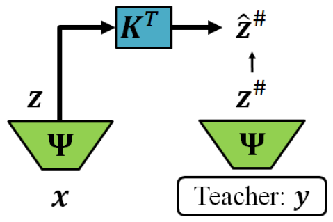
Figure 1: EDMD with dictionary learning architecture

When learning an adaptive dictionary of a fixed size using a neural network (or other function approximation method), let us consider two objects: the dictionary space $\mathcal{S}=\left\{\psi_{j}(\bullet;\boldsymbol{\theta}):\mathbb{R}^{n}\rightarrow\mathbb{R}\enskip:\enskip\forall\boldsymbol{\theta}\in\Theta,\enskip j=1,\ldots,d\right\}$ is the set of all functions which can be parameterized by the neural network and the dictionary $\mathcal{D}(\boldsymbol{\theta})=\left\{\psi_{j}(\bullet;\boldsymbol{\theta}):\mathbb{R}^{n}\rightarrow\mathbb{R}\enskip:\enskip j=1,\ldots,d\right\}$ is the $d$ elements of $\mathcal{S}$ fixed by choosing $\boldsymbol{\theta}$. In EDMD and the dictionary learning approach just described, the Koopman operator is always approximated on a subspace $\mathcal{F}_{\mathbf{X}}=\left\{\mathbf{\Psi}^{*}\mathbf{w}\enskip:\enskip\mathbf{w}\in\mathcal{R}(\mathbf{\Psi}_{\mathbf{X}})\right\}\subset\mathcal{F}_{\mathcal{D}}=\operatorname{span}\mathcal{D}$. As discussed earlier, the EDMD method always uses $\mathcal{S}=\mathcal{D}$ and the only way to increase resolution and feature complexity is to grow the dictionary — leading to the over-fitting problems illustrated in Example 2.1. By contrast, the dictionary learning approach enables us to keep the size of the dictionary relatively small while exploring a much larger space $\mathcal{S}$. In particular, the dictionary size is presumed to be much smaller than the total number of training data points and probably small enough so that $\mathcal{F}_{\mathbf{X}}=\mathcal{F}_{\mathcal{D}}$. Otherwise, the number of functions $d$ learned by the network could be reduced so that this becomes true. The small dictionary size therefore prevents the method from memorizing the snapshot pairs without learning true invariant subspaces. This is not done at the expense of resolution since the allowable complexity of functions in $\mathcal{S}$ is extremely high.

Deep neural networks are advantageous since they enable highly efficient representations of certain natural classes of complex features [23, 14]. In particular, deep neural networks are capable of learning functions whose values are built by applying many simple operations in succession. It is shown empirically that this is indeed an important and natural class of functions since deep neural networks have recently enabled near human level performance on tasks like image and handwritten digit recognition [7]. This proved to be a useful property for dictionary learning for EDMD since [37, 13] achieve state of the art results on examples including the Duffing equation, Kuramoto-Sivashinsky PDE, a system representing the glycolysis pathway, and power systems.

4 New approach: deep feature learning using the LRAN

By removing the constraint that the full state observable is in the learned Koopman invariant subspace, one can do even better. This is especially important for high-dimensional systems where it would be prohibitive to train such a large neural network-based dictionary with limited training data. Furthermore, it may simply not be the case that the full state observable lies in a finite-dimensional Koopman invariant subspace. The method described here is capable of learning extremely low-dimensional invariant subspaces limited only by the intrinsic dimensionality of linearly-evolving patterns in the data. A schematic of our general architecture is presented in Fig. 2. The dictionary function values are given by the output of an encoder neural network $\mathbf{z}=\mathbf{\Psi}(\mathbf{x};\boldsymbol{\theta}_{enc})$ parameterized by $\boldsymbol{\theta}_{enc}$. We avoid the trivial solution by nonlinearly reconstructing an approximation of the full state using a decoder neural network $\hat{\mathbf{x}}=\tilde{\mathbf{\Psi}}(\mathbf{z};\boldsymbol{\theta}_{dec})$ parameterized by $\boldsymbol{\theta}_{dec}$. The decoder network takes the place of Koopman modes for reconstructing the full state from eigenfunction values. However, if Koopman modes are desired it is still possible to compute them using two methods. The first is to employ the same regression procedure whose solution is given by Eq. 18 to compute the Koopman modes from the EDMD dictionary provided by the encoder. Reconstruction using the Koopman modes will certainly achieve lower accuracy than the nonlinear decoder, but may still provide a useful tool for feature extraction and visualization. The other option is to employ a linear decoder network $\tilde{\mathbf{\Psi}}(\mathbf{z};\boldsymbol{\theta}_{dec})=\mathbf{B}(\boldsymbol{\theta}_{dec})\mathbf{z}$ where $\mathbf{B}(\boldsymbol{\theta}_{dec})\in\mathbb{R}^{n\times d}$ is a matrix whose entries are parameterized by $\boldsymbol{\theta}_{dec}$. The advantage of using a nonlinear decoder network is that the full state observable need not be in the span of the learned encoder dictionary functions. A nonlinear decoder can reconstruct more information about the full state from fewer features provided by the encoder. This enables the dictionary size $d$ to be extremely small — yet informative enough to enable nonlinear reconstruction. This is exactly the principle underlying the success of undercomplete autoencoders for feature extraction, manifold learning, and dimensionality reduction. Simultaneous training of the encoder and decoder networks extract rich dictionary elements which the decoder can use for reconstruction.

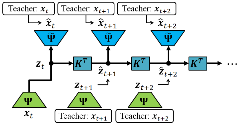
Figure 2: Linearly-Recurrent Autoencoder Network (LRAN) architecture

The technique includes a linear time evolution process given by the matrix $\mathbf{K}(\boldsymbol{\theta}_{\mathbf{K}})$ parameterized by $\boldsymbol{\theta}_{\mathbf{K}}$. This matrix furnishes our approximation of the Koopman operator on the learned dictionary. Taking the eigendecomposition $\mathbf{K}=\mathbf{W}_{R}\mathbf{\Lambda}\mathbf{W}_{L}^{*}$ allows us to compute the Koopman eigenvalues, eigenfunctions, and modes exactly as we would for EDMD using Eq. 15 and Eq. 18. By training the operator $\mathbf{K}$ simultaneously with the encoder and decoder networks, the dictionary of observables learned by the encoder is forced to span a low-dimensional Koopman invariant subspace which is sufficiently informative to approximately reconstruct the full state. In many real-world applications, the scientist has access to data sets consisting of several sequential snapshots. The LRAN architecture shown in Fig. 2 takes advantage of longer sequences of snapshots during training. This is especially important when the system dynamics are highly non-normal. In such systems, low-amplitude features which could otherwise be ignored for reconstruction purposes are highly observable and influence the larger amplitude dynamics several time-steps into the future. One may be able to achieve reasonable accuracy on snapshot pairs by neglecting some of these low-energy modes, but accuracy will suffer as more time steps are predicted. Inclusion of multiple time steps where possible forces the LRAN to incorporate these dynamically important non-normal features in the dictionary. As we will discuss later, it is possible to generalize the LRAN architecture to continuous time systems with irregular sampling intervals and sequence lengths. It is also possible to restrict the LRAN to the case when only snapshot pairs are available. Here we consider the case when our data contains equally-spaced snapshot sequences $\left\{\mathbf{x}_{t},\mathbf{x}_{t+1},\ldots,\mathbf{x}_{t+\mathcal{T}-1}\right\}$ of length $\mathcal{T}$. The loss function

(25) $$J(\boldsymbol{\theta}_{enc},\boldsymbol{\theta}_{dec},\boldsymbol{\theta}_{\mathbf{K}})=\operatorname*{\!\mathbb{E}\enskip}_{\mathbf{x}_{t},\ldots,\mathbf{x}_{t+\mathcal{T}-1}\sim P_{data}}\frac{1}{1+\beta}\biggl{[}\sum_{\tau=0}^{\mathcal{T}-1}\frac{\delta^{t}}{N_{1}(\delta)}\frac{\left\|\hat{\mathbf{x}}_{t+\tau}-\mathbf{x}_{t+\tau}\right\|^{2}}{\left\|\mathbf{x}_{t+\tau}\right\|^{2}+\epsilon_{1}}\\ +\beta\sum_{\tau=1}^{\mathcal{T}-1}\frac{\delta^{t-1}}{N_{2}(\delta)}\frac{\left\|\hat{\mathbf{z}}_{t+\tau}-\mathbf{z}_{t+\tau}\right\|^{2}}{\left\|\mathbf{z}_{t+\tau}\right\|^{2}+\epsilon_{2}}\biggr{]}+\Omega(\boldsymbol{\theta}_{enc},\boldsymbol{\theta}_{dec},\boldsymbol{\theta}_{\mathbf{K}})$$

is minimized during training, where $\mathbb{E}$ denotes the expectation over the data distribution. The encoding, latent state dynamics, and decoding processes are given by

$$\mathbf{z}_{t+\tau}=\mathbf{\Psi}(\mathbf{x}_{t+\tau};\boldsymbol{\theta}_{enc}),\quad\hat{\mathbf{z}}_{t+\tau}=\left[\mathbf{K}(\boldsymbol{\theta}_{\mathbf{K}})^{\tau}\right]^{T}\mathbf{z}_{t},\quad\hat{\mathbf{x}}_{t+\tau}=\tilde{\mathbf{\Psi}}(\hat{\mathbf{z}}_{t+\tau};\boldsymbol{\theta}_{dec}),$$

respectively. The regularization term $\Omega$ has been included for generality, though our numerical experiments show that it was not necessary. Choosing a small dictionary size $d$ provides sufficient regularization for the network. The loss function Eq. 25 consists of a weighted average of the reconstruction error and the hidden state time evolution error. The parameter $\beta$ determines the relative importance of these two terms. The errors themselves are relative square errors between the predictions and the ground truth summed over time with a decaying weight $0<\delta\leq 1$. This decaying weight is used to facilitate training by prioritizing short term predictions. The corresponding normalizing constants,

$$N_{1}(\delta)=\sum_{\tau=0}^{\mathcal{T}-1}\delta^{\tau},\qquad N_{2}(\delta)=\sum_{\tau=1}^{\mathcal{T}-1}\delta^{\tau-1}$$

ensure that the decay-weighted average is being taken over time. The small constants $\epsilon_{1}$ and $\epsilon_{2}$ are used to avoid division by $0$ in the case that the ground truth values vanish. The expectation value was estimated empirically using minibatches consisting of sequences of length $\mathcal{T}$ drawn randomly from the training data. Stochastic gradient descent with the Adaptive Moment Estimation (ADAM) method and slowly decaying learning rate was used to simultaneously optimize the parameters $\boldsymbol{\theta}_{enc}$, $\boldsymbol{\theta}_{dec}$, and $\boldsymbol{\theta}_{\mathbf{K}}$ in the open-source software package TensorFlow.

4.1 Neural network architecture and initialization

The encoder and decoder consist of deep neural networks whose schematic is sketched in Fig. 3. The figure is only a sketch since many more hidden layers were actually used in the architectures applied to example problems in this paper. In order to achieve sufficient depth in the encoder and decoder networks, hidden layers employed exponential linear units or “elu’s” as the nonlinearity [3]. These units mitigate the problem of vanishing and exploding gradients in deep networks by employing the identity function for all non-negative arguments. A shifted exponential function for negative arguments is smoothly matched to the linear section at the origin, giving the activation function

(26) $$\operatorname{elu}(x)=\begin{cases}x&\quad x\geq 0\\ \exp(x)-1&\quad x<0\end{cases}.$$

This prevents the units from “dying” as standard rectified linear units or “ReLU’s” do when the arguments are always negative on the data. Furthermore, “elu’s” have the advantage of being continuously differentiable. This will be a nice property if we want to approximate a $C^{1}$ data manifold whose chart map and its inverse are given by the encoder and decoder. If the maps are differentiable, then the tangent spaces can be defined as well as push-forward, pull-back, and connection forms. Hidden layers map the activations $\mathbf{x}^{(l)}$ at layer $l$ to activations at the next layer $l+1$ given by a linear transformation and subsequent element-wise application of the activation function,

(27) $$\mathbf{x}^{(l+1)}=\operatorname{elu}\left[\mathbf{W}^{(l)}(\boldsymbol{\theta})\mathbf{x}^{(l)}+\mathbf{b}^{(l)}(\boldsymbol{\theta})\right],\quad\mathbf{W}^{(l)}(\boldsymbol{\theta})\in\mathbb{R}^{n_{l+1}\times n_{l}},\quad\mathbf{b}^{(l)}(\boldsymbol{\theta})\in\mathbb{R}^{n_{l+1}}.$$

The weight matrices $\mathbf{W}$ and vector biases $\mathbf{b}$ parameterized by $\boldsymbol{\theta}$ are learned by the network during training. The output layers $L$ for both the encoder and decoder networks utilize linear transformations without a nonlinear activation function:

(28) $$\mathbf{x}^{(L)}=\mathbf{W}^{(L-1)}(\boldsymbol{\theta})\mathbf{x}^{(L-1)}+\mathbf{b}^{(L-1)}(\boldsymbol{\theta}),\quad\mathbf{W}^{(L-1)}(\boldsymbol{\theta})\in\mathbb{R}^{n_{L}\times n_{L-1}},\quad\mathbf{b}^{(L-1)}(\boldsymbol{\theta})\in\mathbb{R}^{n_{L}},$$

where $L=L_{enc}$ or $L=L_{dec}$ is the last layer of the encoder or decoder with $n_{L_{enc}}=d$ or $n_{L_{dec}}=n$ respectively. This allows for smooth and consistent treatment of positive and negative output values without limiting the flow of gradients back through the network.

The weight matrices were initialized using the Xavier initializer in Tensorflow. This initialization distributes the entries in $\mathbf{W}^{(l)}$ uniformly over the interval $[-\alpha,\alpha]$ where $\alpha=\sqrt{6/(n_{l}+n_{l+1})}$ in order to keep the scale of gradients approximately the same in all layers. This initialization method together with the use of exponential linear units allowed deep networks to be used for the encoder and decoder. The bias vectors $\mathbf{b}^{(l)}$ were initialized to be zero. The transition matrix $\mathbf{K}$ was initialized to have diagonal blocks of the form $\begin{bmatrix}\sigma&\omega\\ -\omega&\sigma\end{bmatrix}$ with eigenvalues $\lambda=\sigma\pm\omega\imath$ equally spaced around the circle of radius $r=\sqrt{\sigma^{2}+\omega^{2}}=0.8$. This was done heuristically to give the initial eigenvalues good coverage of the unit disc. One could also initialize this matrix using a low-rank DMD matrix.

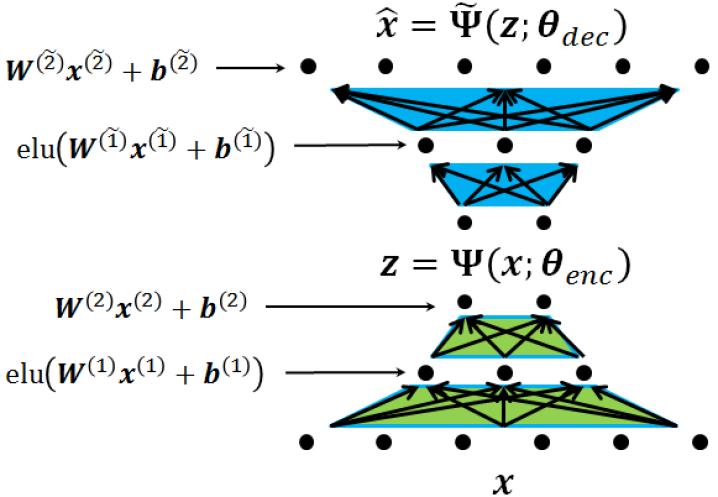
Figure 3: Architecture of the encoder and decoder networks

4.2 Simple modifications of LRANs

Several extensions and modifications of the LRAN architecture are possible. Some simple modifications are discussed here, with several more involved extensions suggested in the conclusion. In the first extension, we observe that it is easy learn Koopman eigenfunctions associated with known eigenvalues simply by fixing the appropriate entries in the matrix $\mathbf{K}$. In particular, if we know that our system has Koopman eigenvalue $\mu=\sigma+\omega\imath$ then we may formulate the state transition matrix

(29) $$\mathbf{K}(\boldsymbol{\theta})=\begin{bmatrix}\begin{bmatrix}\sigma&\omega\\ -\omega&\sigma\end{bmatrix}&\mathbf{0}_{2\times(d-2)}\\ \mathbf{0}_{(d-2)\times 2}&\tilde{\mathbf{K}}(\boldsymbol{\theta})\end{bmatrix}.$$

In the above, the known eigenvalue is fixed and only the entries of $\tilde{\mathbf{K}}$ are allowed to be trained. If more eigenvalues are known, we simply fix the additional entries of $\mathbf{K}$ in the same way. The case where some eigenvalues are known is particularly interesting because in certain cases, eigenvalues of the linearized system are Koopman eigenvalues whose eigenfunctions have useful properties. Supposing the autonomous system under consideration has a fixed point with all eigenvalues $\mu_{i}$, $i=1,\ldots,n$ inside the unit circle, the Hartman-Grobman theorem establishes a topological conjugacy to a linear system with the same eigenvalues in a small neighborhood $\mathcal{U}$ of the fixed point. One easily checks that the coordinate transformations $h_{i}:\mathcal{M}\cap\mathcal{U}\rightarrow\mathbb{R}$, $i=1,\ldots,n$ establishing this conjugacy are Koopman eigenfunctions restricted to the neighborhood. Composing them with the flow map allows us to extend the eigenfunctions to the entire basin of attraction by defining $\varphi_{i}(\mathbf{x})=\mu_{i}^{-\tau(\mathbf{x})}h_{i}\left(\mathbf{f}^{\tau(\mathbf{x})}(\mathbf{x})\right)$ where $\tau(\mathbf{x})$ is the smallest integer $\tau$ such that $\mathbf{f}^{\tau}(\mathbf{x})\in\mathcal{U}$. These eigenfunctions extend the topological conjugacy by parameterizing the basin. Similar results hold for stable limit cycles and tori [20]. This is nice because we can often find eigenvalues at fixed points explicitly by linearization. Choosing to fix these eigenvalues in the $\mathbf{K}$ matrix forces the LRAN to learn corresponding eigenfunctions parameterizing the basin of attraction. It is also easy to include a set of observables explicitly by appending them to the encoder function $\mathbf{\Psi}(\mathbf{x};\boldsymbol{\theta}_{enc})=\left[\mathbf{\Psi}_{fixed}(\mathbf{x})^{T},\enskip\tilde{\mathbf{\Psi}}(\mathbf{x};\boldsymbol{\theta}_{enc})^{T}\right]^{T}$ so that only the functions $\tilde{\mathbf{\Psi}}$ are learned by the network. This may be useful if we want to accurately reconstruct some observables $\mathbf{\Psi}_{fixed}$ linearly using Koopman modes.

The LRAN architecture and loss function Eq. 25 may be further generalized to non-uniform sampling of continuous-time systems. In this case, we consider $T$ sequential snapshots
$\left\{\mathbf{x}(t_{0}),\mathbf{x}(t_{1}),\ldots,\mathbf{x}(t_{T-1})\right\}$ where the times $t_{0},t_{1},\ldots,t_{T-1}$ are not necessarily evenly spaced. In the continuous time case, we have a Koopman operator semigroup $\mathcal{K}_{t+s}=\mathcal{K}_{t}\mathcal{K}_{s}$ defined as $\mathcal{K}_{t}\psi(\mathbf{x})=\psi(\mathbf{\varPhi}_{t}(\mathbf{x}))$ and generated by the operator $\mathcal{K}\psi(\mathbf{x})=\dot{\psi}(\mathbf{x})=\left(\nabla_{\mathbf{x}}\psi(\mathbf{x})\right)\mathbf{f}(\mathbf{x})$ where the dynamics are given by $\dot{\mathbf{x}}=\mathbf{f}(\mathbf{x})$ and $\mathbf{\varPhi}_{t}$ is the time $t$ flow map. The generator $\mathcal{K}$ is clearly a linear operator which we can approximate on our dictionary of observables with a matrix $\mathbf{K}$. By integrating, we can approximate elements from the semigroup $\mathcal{K}_{t}$ using the matrices $\mathbf{K}_{t}=\exp{(\mathbf{K}t)}$ on the dictionary. Finally, in order to formulate the analogous loss function, we might utilize continuously decaying weights

(30) $$\rho_{1}(t)=\frac{\delta^{t}}{\sum_{k=0}^{\mathcal{T}-1}\delta^{t_{k}}},\qquad\rho_{2}(t)=\frac{\delta^{t}}{\sum_{k=1}^{\mathcal{T}-1}\delta^{t_{k}}},$$

normalized so that they sum to $1$ for the given sampling times. Neural networks can be used for the encoder and decoder together with the loss function

(31) $$J(\boldsymbol{\theta}_{enc},\boldsymbol{\theta}_{dec},\boldsymbol{\theta}_{\mathbf{K}})=\operatorname*{\!\mathbb{E}\enskip}_{\mathbf{x}(t_{0}),\ldots,\mathbf{x}(t_{\mathcal{T}-1})\sim P_{data}}\frac{1}{1+\beta}\biggl{[}\sum_{k=0}^{\mathcal{T}-1}\rho_{1}(t_{k})\frac{\left\|\hat{\mathbf{x}}(t_{k})-\mathbf{x}(t_{k})\right\|^{2}}{\left\|\mathbf{x}(t_{k})\right\|^{2}+\epsilon_{1}}\\ +\beta\sum_{k=1}^{\mathcal{T}-1}\rho_{2}(t_{k})\frac{\left\|\hat{\mathbf{z}}(t_{k})-\mathbf{z}(t_{k})\right\|^{2}}{\left\|\mathbf{z}(t_{k})\right\|^{2}+\epsilon_{2}}\biggr{]}+\Omega(\boldsymbol{\theta}_{enc},\boldsymbol{\theta}_{dec},\boldsymbol{\theta}_{\mathbf{K}})$$

to be minimized during training. In this case, the dynamics evolve the observables linearly in continuous time, so we let

$$\mathbf{z}(t_{k})=\mathbf{\Psi}(\mathbf{x}(t_{k});\boldsymbol{\theta}_{enc}),\quad\hat{\mathbf{z}}(t_{k})=\exp\left[\mathbf{K}(\boldsymbol{\theta}_{\mathbf{K}})(t_{k}-t_{0})\right]^{T}\mathbf{z}(t_{0}),\quad\hat{\mathbf{x}}(t_{k})=\tilde{\mathbf{\Psi}}(\hat{\mathbf{z}}(t_{k});\boldsymbol{\theta}_{dec}).$$

This loss function can be evaluated on the training data and minimized in essentially the same way as Eq. 25. The only difference is that we are discovering a matrix approximation to the generator of the Koopman semigroup. We will not explore irregularly sampled continuous time systems further in this paper, leaving it as a subject for future work.

We briefly remark that the general LRAN architecture can be restricted to the case of snapshot pairs as shown in Fig. 4. In this special case, training might be accelerated using a technique similar to Algorithm 1. During the initial stage of training, it may be beneficial to periodically re-initialize the $\mathbf{K}$ matrix with its EDMD approximation using the current dictionary functions and a subset of the training data. This might provide a more suitable initial condition for the matrix as well as accelerate the training process. However, this update for $\mathbf{K}$ is not consistent with all the terms in the loss function $J$ since it does not account for reconstruction errors. Therefore, the final stages of training must always proceed by gradient descent on the complete loss function.

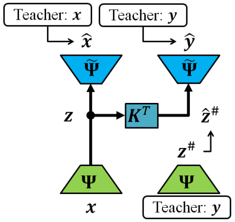
Figure 4: LRAN architecture restricted to snapshot pairs

Finally, we remark that the LRAN architecture sacrifices linear reconstruction using Koopman modes for nonlinear reconstruction using a decoder neural network in order to learn ultra-low dimensional Koopman invariant subspaces. Interestingly, this formulation allows the LRAN to parameterize the Nonlinear Normal Modes (NNMs) frequently encountered in structural dynamics. These modes are two-dimensional, periodic invariant manifolds containing a fixed point of a Hamiltonian system lacking internal resonances. Therefore, if $\mu=\omega\imath$ and $\overline{\mu}=-\omega\imath$ are a complex conjugate pair of pure imaginary eigenvalues of $\mathbf{K}$ with corresponding left eigenvectors $\mathbf{w}_{L}$ and $\overline{\mathbf{w}_{L}}$ then a NNM is parameterized as follows:

(32) $$\mathbf{x}(\alpha)=\tilde{\mathbf{\Psi}}(\alpha\mathbf{w}_{L}+\overline{\alpha\mathbf{w}_{L}};\boldsymbol{\theta}_{dec})=\tilde{\mathbf{\Psi}}\left(2\Re(\alpha)\Re(\mathbf{w}_{L})-2\Im(\alpha)\Im(\mathbf{w}_{L});\boldsymbol{\theta}_{dec}\right).$$

The global coordinates on the manifold are $\left(\Re(\alpha),\Im(\alpha_{2})\right)$. Coordinate projection of the full state onto the NNM,

(33) $$\begin{bmatrix}\Re(\alpha)\\ \Im(\alpha)\end{bmatrix}=\begin{bmatrix}\Re(\mathbf{w}_{R})^{T}\\ \Im(\mathbf{w}_{R})^{T}\end{bmatrix}\mathbf{\Psi}(\mathbf{x};\boldsymbol{\theta}_{enc}),$$

is accomplished by employing the encoder network and the right eigenvector $\mathbf{w}_{R}$ corresponding to eigenvalue $\mu$. These coordinates are the real and imaginary parts of the associated Koopman eigenfunction $\alpha=\varphi(\mathbf{x})$. The NNM has angular frequency $\angle(\omega\imath)/\Delta t$ where $\Delta t$ is the sampling interval between the snapshots in the case of the discrete time LRAN.

We may further generalize the notion of NNMs by considering the Koopman mode expansion of the real-valued observable vector $\mathbf{\Psi}$ making up our dictionary. In this particular case, the associated Koopman modes are the complex conjugate left eigenvectors of $\mathbf{K}$. They allow exact reconstruction and prediction using the decomposition

(34) $$\mathbf{z}_{t}=\sum_{j=1}^{r}\overline{\mathbf{w}_{L,j}}\mu_{j}^{t}\left(\mathbf{w}_{R,j}^{T}\mathbf{z}_{0}\right)=\sum_{j=1}^{r}\overline{\mathbf{w}_{L,j}}\mu_{j}^{t}\varphi_{j}(\mathbf{x}_{0}),$$

assuming a Koopman invariant subspace has been learned that contains the full state observable. Reconstructing and predicting with the decoder instead, we have

(35) $$\mathbf{x}_{t}=\tilde{\mathbf{\Psi}}\left[\sum_{j=1}^{r}\overline{\mathbf{w}_{L,j}}\mu_{j}^{t}\varphi_{j}(\mathbf{x}_{0});\enskip\boldsymbol{\theta}_{dec}\right].$$

Therefore, each invariant subspace of $\mathbf{K}$ given by its left eigenvectors corresponds to an invariant manifold in the $n$-dimensional phase space. These manifolds have global charts whose coordinate projections are given by the Koopman eigenfunctions $\varphi_{j}(\mathbf{x})=\mathbf{w}_{R,j}^{T}\mathbf{\Psi}(\mathbf{x};\boldsymbol{\theta}_{enc})$. The dynamics on these manifolds is incredibly simple and entails repeated multiplication of the coordinates by the eigenvalues. Generalized eigenspaces may also be considered in the natural way by using the Jordan normal form of $\mathbf{K}$ instead of its eigendecomposition in the above arguments. The only necessary change is in the evolution equations, where instead of taking powers of $\mathbf{\Lambda}=\operatorname{diag}\left\{\mu_{1},\ldots,\mu_{r}\right\}$, we take powers of $\mathbf{J}$, the matrix consisting of Jordan blocks [20]. Future work might use a variational autoencoder (VAE) formulation [7, 18, 17, 12] where a given distribution is imposed on the latent state in order to facilitate sampling.

5 EDMD-based model reduction as a shallow autoencoder

In this section we examine how the EDMD method might be used to construct low-dimensional Koopman invariant subspaces while still allowing for accurate reconstructions and predictions of the full state. The idea is to find a reduced order model of the large linear system identified by EDMD in the space of observables. This method is sometimes called overspecification [26] and essentially determines an encoder function into an appropriate small set of features. From this reduced set of features, we then employ nonlinear reconstruction of the full state through a learned decoder function. Introduction of the nonlinear decoder should allow for lower-dimensional models to be identified which are still able to make accurate predictions. The proposed framework therefore constructs a kind of autoencoder where encoded features evolve with linear time invariant dynamics. The encoder functions are found explicitly as linear combinations of EDMD observables and are therefore analogous to a shallow neural network with a single hidden layer. The nonlinear decoder function is also found explicitly through a regression process involving linear combinations of basis functions.

We remark that this approach differs from training an LRAN by minimization of Eq. 25 in two important ways. First, the EDMD-based model reduction and reconstruction processes are performed sequentially; thus, the parts are not simultaneously optimized as in the LRAN. The LRAN is advantageous since we only learn to encode observables which the decoder can successfully use for reconstruction. There are no such guarantees here. Second, the EDMD dictionary remains fixed albeit overspecified whereas the LRAN explicitly learns an appropriate dictionary. Therefore, the EDMD shallow autoencoder framework will still suffer from the overfitting problem illustrated in Example 2.1. If the EDMD-identified matrix $\mathbf{K}$ does not correctly represent the dynamics on a Koopman invariant subspace, then any reduced order models derived from it cannot be expected to be accurately relect the dynamics either. Nonetheless, in many cases, this method could provide a less computationally expensive alternative to training a LRAN which retains some of the benefits owing to nonlinear reconstruction.

Dimensionality reduction is achieved by first performing EDMD with a large dictionary, then projecting the linear dynamics onto a low-dimensional subspace. A naive approach would be to simply project the large feature space system onto the most energetic POD modes — equivalent to low-rank truncation of the SVD $\mathbf{\Psi}_{\mathbf{X}}=\mathbf{U}\mathbf{\Sigma}\mathbf{V}^{*}$. While effective for normal systems with a few dominant modes, this approach yields very poor predictions in non-normal systems since low amplitude modes with large impact on the dynamics would be excluded from the model. One method which resolves this issue is balanced truncation of the identified feature space system. Such an idea is suggested in [26] for reducing the system identified by linear DMD. Drawing from the model reduction procedure for snapshot-based realizations developed in [15], we will construct a balanced reduced order model for the system identified using EDMD or KDMD. In the formulation of EDMD that led to the kernel method, an approximation of the Koopman operator,

(36) $$\mathcal{K}\mathbf{\Psi}(\mathbf{x})^{*}\mathbf{a}=\mathbf{\Psi}(\mathbf{x})^{*}\mathbf{U}\hat{\mathbf{K}}\mathbf{U}^{*}\mathbf{a}+\mathbf{r}(\mathbf{x}),\quad\forall\mathbf{a}\in\mathcal{R}(\mathbf{U}),$$

was obtained. The approximation allows us to model the dynamics of a vector of observables,

(37) $$\mathbf{\Psi}_{\mathbf{U}}(\mathbf{x})=\mathbf{U}^{*}\mathbf{\Psi}(\mathbf{x})=\mathbf{\Sigma}^{+}\mathbf{V}^{*}\mathbf{\Psi}_{\mathbf{X}}^{*}\mathbf{\Psi}(\mathbf{x}),$$

with the linear input-output system

(38) $$\begin{aligned} \mathbf{\Psi}_{\mathbf{U}}(\mathbf{x}_{t+1})&=\hat{\mathbf{K}}^{*}\mathbf{\Psi}_{\mathbf{U}}(\mathbf{x}_{t})+\dfrac{1}{\sqrt{M}}\mathbf{\Sigma}\mathbf{u}_{t}\\ \mathbf{x}_{t}&=\mathbf{C}\mathbf{\Psi}_{\mathbf{U}}(\mathbf{x}_{t})\end{aligned},$$

where $\hat{\mathbf{K}}$ is the matrix Eq. 14 identified by EDMD or KDMD. The input $\mathbf{u}_{t}$ is provided in order to equate varying initial conditions $\mathbf{\Psi}_{\mathbf{U}}(\mathbf{x}_{0})$ with impulse responses of Eq. 38. Since the input is used to set the initial condition, we choose to scale each component by its singular value to reflect the covariance

(39) $$\operatorname*{\!\mathbb{E}\enskip}_{\mathbf{x}\sim P_{data}}\left[\mathbf{\Psi}_{\mathbf{U}}(\mathbf{x})\mathbf{\Psi}_{\mathbf{U}}(\mathbf{x})^{*}\right]\approx\frac{1}{M}\mathbf{U}^{*}\mathbf{\Psi}_{\mathbf{X}}\mathbf{\Psi}_{\mathbf{X}}^{*}\mathbf{U}=\frac{1}{M}\mathbf{\Sigma}^{2}=\operatorname*{\!\mathbb{E}\enskip}_{\mathbf{u}\sim\mathcal{N}(\mathbf{0},\mathbf{I}_{r})}\left[\dfrac{1}{M}\mathbf{\Sigma}\mathbf{u}\mathbf{u}^{*}\mathbf{\Sigma}^{*}\right],$$

in the observed data. Therefore, initializing the system using impulse responses $\mathbf{u}_{0}=\mathbf{e}_{j}$, $j=1,\ldots,r$ from the $\sigma$-points of the distribution $\mathbf{u}\sim\mathcal{N}(\mathbf{0},\mathbf{I}_{r})$ ensures that the correct empirical covariances are obtained. The output matrix,

(40) $$\mathbf{C}=\mathbf{X}\mathbf{V}\mathbf{\Sigma}^{+},$$

is used to linearly reconstruct the full state observable from the complete set of features. It is found using linear regression similar to the Koopman modes Eq. 18. The low-dimensional set of observables making up the encoder will be found using a balanced reduced order model of Eq. 38.

5.1 Balanced Model Reduction

Balanced truncation [21] is a projection-based model reduction techniqe that attempts to retain a subspace in which Eq. 38 is both maximally observable and controllable. While these notions generally do not coincide in the original space, remarkably it is possible to find a left-invertible linear transformation $\mathbf{\Psi}_{\mathbf{U}}(\mathbf{x})=\mathbf{T}\mathbf{z}$ under which these properties are balanced. This so called balancing transformation of the learning subspace simultaneously diagonalizes the observability and controllability Gramians. Therefore, the most observable states are also the most controllable and vice versa. The reduced order model is formed by truncating the least observable/controllable states of the transformed system. If the discrete time observability Gramian $\mathbf{W}_{o}$ and controllability Gramian $\mathbf{W}_{c}$ are given by

(41) $$\mathbf{W}_{o}=\sum_{t=0}^{\infty}(\hat{\mathbf{K}})^{t}\mathbf{C}^{*}\mathbf{C}(\hat{\mathbf{K}}^{*})^{t},\qquad\mathbf{W}_{c}=\frac{1}{M}\sum_{t=0}^{\infty}(\hat{\mathbf{K}}^{*})^{t}\mathbf{\Sigma}^{2}(\hat{\mathbf{K}})^{t},$$

then the Gramians transform according to

(42) $$\mathbf{W}_{o}\mapsto\mathbf{T}^{*}\mathbf{W}_{o}\mathbf{T},\qquad\mathbf{W}_{c}\mapsto\mathbf{T}_{L}^{+}\mathbf{W}_{c}(\mathbf{T}_{L}^{+})^{*}$$

under the change of coordinates. In the above, $\mathbf{S}^{*}=\mathbf{T}_{L}^{+}$ is the left pseudoinverse satisfying $\mathbf{S}^{*}\mathbf{T}=\mathbf{I}_{d}$ where $d$ is the rank of $\mathbf{T}$ and $\mathbf{T}\mathbf{S}^{*}=\mathbf{P}_{\mathbf{T}}$ is a (not necessarily orthogonal) projection operator onto $\mathcal{R}(\mathbf{T})$.

Since the Gramians are Hermitian positive semidefinite, they can be written as $\mathbf{W}_{o}=\mathbf{A}\mathbf{A}^{*}$, $\mathbf{W}_{c}=\mathbf{B}\mathbf{B}^{*}$ for some not necessarily unique matrices $\mathbf{A},\mathbf{B}\in\mathbb{R}^{r\times r}$. Forming an economy sized singular value decomposition $\mathbf{H}=\mathbf{A}^{*}\mathbf{B}=\mathbf{U}_{H}\mathbf{\Sigma}_{H}\mathbf{V}_{H}$ allows us to construct the transformations

(43) $$\mathbf{T}=\mathbf{B}\mathbf{V}_{H}(\mathbf{\Sigma}_{H}^{+})^{1/2},\qquad\mathbf{S}=\mathbf{A}\mathbf{U}_{H}(\mathbf{\Sigma}_{H}^{+})^{1/2}.$$

Using this construction, it is easy to check that the resulting transformation simultaneously diagonalizes the Gramians:

(44) $$\mathbf{T}^{*}\mathbf{W}_{o}\mathbf{T}=\mathbf{S}^{*}\mathbf{W}_{c}\mathbf{S}=\mathbf{\Sigma}_{H}.$$

Entries of the diagonal matrix $\mathbf{\Sigma}_{H}$ are called the Hankel singular values. The columns of $\mathbf{T}$ and $\mathbf{S}$ are called the “balancing modes” and “adjoint modes” respectively. The balancing modes span the subspace where Eq. 38 is both observable and controllable while the adjoint modes furnish the projected coefficients of the state $\mathbf{S}^{*}\mathbf{\Psi}_{\mathbf{U}}(\mathbf{x})=\mathbf{z}$ onto the space where these properties are balanced. The corresponding Hankel singular values quantify the observability/controllability of the states making up $\mathbf{z}$. Therefore, a reduced order model which is provably close to optimal truncation in the $\mathcal{H}_{\infty}$ norm is formed by rank-$d$ truncation of the SVD, retaining only the first $d$ balancing and adjoint modes $\mathbf{T}_{d}$ and $\mathbf{S}_{d}$ [4]. The reduced state space system modeling the dynamics of Eq. 38 is given by

(45) $$\begin{aligned} \mathbf{z}_{t+1}&=\mathbf{S}_{d}^{*}\hat{\mathbf{K}}^{*}\mathbf{T}_{d}\mathbf{z}_{t}+\dfrac{1}{\sqrt{M}}\mathbf{S}_{d}^{*}\mathbf{\Sigma}\mathbf{u}_{t}\\ \mathbf{x}_{t}&\approx\mathbf{C}\mathbf{T}_{d}\mathbf{z}_{t}\end{aligned},\quad\mbox{where}\quad\mathbf{z}\triangleq\mathbf{S}_{d}^{*}\mathbf{\Psi}_{\mathbf{U}}(\mathbf{x}).$$

Therefore, the reduced dictionary of observables is given by the components of $\mathbf{S}_{d}^{*}\mathbf{\Psi}_{\mathbf{U}}:\mathbb{R}^{n}\rightarrow\mathbb{R}^{d}$ and the corresponding EDMD approximation of the Koopman operator on its span is given by $\mathbf{T}_{d}^{*}\hat{\mathbf{K}}\mathbf{S}_{d}$. This set of features is highly observable in that their dynamics strongly influences the full state reconstruction over time through $\mathbf{C}$. And highly controllable in that the features are excited by typical state configurations through $\mathbf{\Sigma}$. The notion of feature excitation corresponding to controllability will be made clear in the next section.

5.2 Finite-horizon Gramians and Balanced POD

Typically one would find the infinite horizon Gramians for an overspecified Hurwitz EDMD system Eq. 38 by solving the Lyapunov equations

(46) $$\hat{\mathbf{K}}\mathbf{W}_{o}\hat{\mathbf{K}}^{*}-\mathbf{W}_{o}+\mathbf{C}^{*}\mathbf{C}=0,\qquad\hat{\mathbf{K}}^{*}\mathbf{W}_{c}\hat{\mathbf{K}}-\mathbf{W}_{c}+\mathbf{\Sigma}^{2}=0.$$

In the case of neutrally stable or unstable systems, unique positive definite solutions do not exist and one must use generalized Gramians [38]. When used to form balanced reduced order models, this will always result in the unstable and neutrally stable modes being chosen before the stable modes. This could be problematic for our intended framework since EDMD can identify many spurious and sometimes unstable eigenvalues corresponding to noisy low-amplitude fluctuations. While these noisy modes remain insignificant over finite times of interest, they will dominate EDMD-based predictions over long times. Therefore it makes sense to consider the dominant modes identified by EDMD over a finite time interval of interest. Using finite horizon Gramians reduces the effect of spurious modes on the reduced order model, making it more consistent with the data. The time horizon can be chosen to reflect a desired future prediction time or the number of sequential snapshots in the training data.

The method of Balanced Proper Orthogonal Decomposition or BPOD [24] allows us to find balancing and adjoint modes of the finite horizon system. In BPOD, we observe that the finite-horizon Gramians are empirical covariance matrices formed by evolving the dynamics from impulsive initial conditions for time $\mathcal{T}$. This gives the specific form for matrices

(47) $$\mathbf{A}=\begin{bmatrix}\mathbf{C}^{*}&\hat{\mathbf{K}}\mathbf{C}^{*}&\cdots&(\hat{\mathbf{K}})^{\mathcal{T}}\mathbf{C}^{*}\end{bmatrix},\qquad\mathbf{B}=\dfrac{1}{\sqrt{M}}\begin{bmatrix}\mathbf{\Sigma}&\hat{\mathbf{K}}^{*}\mathbf{\Sigma}&\cdots&(\hat{\mathbf{K}}^{*})^{\mathcal{T}}\mathbf{\Sigma}\end{bmatrix},$$

allowing for computation of the balancing and adjoint modes without ever forming the Gramians. This is known as the method of snapshots. Since the output dimension is large, we consider its projection onto the most energetic modes. These are identified by forming the economy sized SVD of the impulse responses $\mathbf{C}\mathbf{B}=\mathbf{U}_{OP}\mathbf{\Sigma}_{OP}\mathbf{V}_{OP}^{*}$. Projecting the output allows us to form the elements of

(48) $$\mathbf{A}_{OP}=\begin{bmatrix}\mathbf{C}^{*}\mathbf{U}_{OP}&\hat{\mathbf{K}}\mathbf{C}^{*}\mathbf{U}_{OP}&\cdots&(\hat{\mathbf{K}})^{\mathcal{T}}\mathbf{C}^{*}\mathbf{U}_{OP}\end{bmatrix},$$

from fewer initial conditions than $\mathbf{A}$. In particular, the initial conditions are the first few columns of $\mathbf{U}_{OP}$ with the largest singular values [24].

Observe that the unit impulses place the initial conditions precisely at the $\sigma$-points of the data-distribution in features space. If this distribution is Gaussian, then the empirical expectations obtained by evolving the linear system agree with the true expectations taken over the entire data distribution. Therefore, the finite horizon controllability Gramian corresponds to the covariance matrix taken over all time $\mathcal{T}$ trajectories starting at initial data points coming from a Gaussian distribution in feature space. Consequently, controllability in this case corresponds exactly with feature variance or expected square amplitude over time.

We remark that in the infinite-horizon limit $\mathcal{T}\rightarrow\infty$, BPOD converges on a transformation which balances the generalized Gramians introduced in [38]. Application of BPOD to unstable systems is discussed in [6] which provides justification for the approach.

Another option to avoid spurious modes from corrupting the long-time dynamics is to consider pre-selection of EDMD modes which are nearly Koopman invariant. The development of such an accuracy criterion for selecting modes is the subject of a forthcoming paper by H. Zhang and C. W. Rowley. One may then apply balanced model reduction to the feature space system containing only the most accurate modes.

5.3 Nonlinear reconstruction

In truncating the system, we determined a small subspace of observables whose values evolve linearly in time and are both highly observable and controllable. However, most of the less observable low-amplitude modes are removed. The linear reconstruction only allows us to represent data on a low-dimensional subspace of $\mathbb{R}^{n}$. While projection onto this subspace aims to explain most of the data variance and dynamics, it may be the case that the data lies near a curved manifold not fully contained in the subspace. The neglected modes contribute to this additional complexity in the shape of the data in $\mathbb{R}^{n}$. Nonlinear reconstruction of the full state can help account for the complex shape of the data and for neglected modes enslaved to the ones retained.

We consider the regression problem involved in reconstructing the full state $\mathbf{x}$ from a small set of EDMD observables $\mathbf{z}$. Because the previously obtained solution to the EDMD balanced model reduction problem Eq. 45 employs linear reconstruction through matrix $\mathbf{C}\mathbf{T}_{d}$, we expect nonlinearities in the reconstruction to be small with most of the variance being accounted for by linear terms. Therefore, the regression model,

(49) $$\mathbf{x}=\mathbf{C}_{1}\mathbf{z}+\mathbf{C}_{2}\mathbf{\Psi}(\mathbf{z})+\mathbf{e},$$

is formulated based on [5, 36] to include linear and nonlinear components. In the above, $\mathbf{\Psi}:\mathbb{C}^{d}\rightarrow\mathcal{H}$ is a nonlinear feature map into reproducing kernel Hilbert space $\mathcal{H}$ and $\mathbf{C}_{1}:\mathbb{C}^{d}\rightarrow\mathbb{C}^{n}$ and $\mathbf{C}_{2}:\mathcal{H}\rightarrow\mathbb{C}^{n}$ are linear operators. These operators are found by solving the $l^{2}$ regularized optimization problem,

(50) $$\operatorname*{\min\!imize\enskip}_{\mathbf{C}_{1},\mathbf{C}_{2}}J=\left\|\mathbf{X}^{*}-\mathbf{Z}^{*}\mathbf{C}_{1}^{*}-\mathbf{\Psi}_{\mathbf{Z}}^{*}\mathbf{C}_{2}^{*}\right\|_{F}^{2}+\gamma\operatorname{Tr}(\mathbf{C}_{2}\mathbf{C}_{2}^{*}),\qquad\gamma\geq 0,$$

involving the empirical square error on the training data $\left\{(\mathbf{z}_{j},\mathbf{x}_{j})\right\}_{j=1}^{M}$ arranged into columns of the matrices $\mathbf{Z}=\begin{bmatrix}\mathbf{z}_{1}&\cdots&\mathbf{z}_{M}\end{bmatrix}$ and $\mathbf{X}=\begin{bmatrix}\mathbf{x}_{1}&\cdots&\mathbf{x}_{M}\end{bmatrix}$. The regularization penalty is placed only on the coefficients of nonlinear terms to control over-fitting while the linear term, which we expect to dominate, is not penalized. The operator $\mathbf{\Psi}_{\mathbf{Z}}:\mathbb{C}^{M}\rightarrow\mathcal{H}$ forms linear combinations of the data in feature space $\mathbf{v}\mapsto v_{1}\mathbf{\Psi}(\mathbf{z}_{1})+\cdots+v_{M}\mathbf{\Psi}(\mathbf{z}_{M})$. Since $\mathbf{Z}$ and $\mathbf{\Psi}_{\mathbf{Z}}$ are operators with finite ranks $r_{1}$ and $r_{2}\leq M$, we may consider their economy sized singular value decompositions: $\mathbf{Z}=\mathbf{U}_{1}\mathbf{\Sigma}_{1}\mathbf{V}_{1}^{*}$ and $\mathbf{\Psi}_{\mathbf{Z}}=\mathbf{U}_{2}\mathbf{\Sigma}_{2}\mathbf{V}_{2}^{*}$. Observe that it is impossible to infer any components of $\mathcal{R}(\mathbf{C}_{1}^{*})$ orthogonal to $\mathcal{R}(\mathbf{Z})$ since they are annihilated by $\mathbf{Z}^{*}$. Therefore, we apply Occam’s razor and assume that $\mathbf{C}_{1}^{*}=\mathbf{U}_{1}\hat{\mathbf{C}}_{1}^{*}$ for some $\hat{\mathbf{C}}_{1}^{*}\in\mathbb{C}^{r_{1}\times n}$. By the same argument, $\mathcal{R}(\mathbf{C}_{2}^{*})$ cannot have any components orthogonal to $\mathcal{R}(\mathbf{\Psi}_{\mathbf{Z}})$ since they are annihilated by $\mathbf{\Psi}_{\mathbf{Z}}^{*}$ and have a positive contribution to the regularization penalty term $\operatorname{Tr}(\mathbf{C}_{2}\mathbf{C}_{2}^{*})$. Hence, we must also have $\mathbf{C}_{2}^{*}=\mathbf{U}_{2}\hat{\mathbf{C}}_{2}^{*}$ for some $\hat{\mathbf{C}}_{2}^{*}\in\mathbb{C}^{r_{2}\times n}$. Substituting these relationships into Eq. 50 allows it to be formulated as the standard least squares problem

(51) $$\begin{aligned} J&=\left\|\mathbf{X}^{*}-\mathbf{V}_{1}\mathbf{\Sigma}_{1}\hat{\mathbf{C}}_{1}^{*}-\mathbf{V}_{2}\mathbf{\Sigma}_{2}\hat{\mathbf{C}}_{2}^{*}\right\|_{F}^{2}+\gamma\left\|\hat{\mathbf{C}}_{2}\right\|_{F}^{2}\\ &=\left\|\begin{bmatrix}\mathbf{X}^{*}\\ \mathbf{0}_{r_{2}\times n}\end{bmatrix}-\begin{bmatrix}\mathbf{V}_{1}\mathbf{\Sigma}_{1}&\mathbf{V}_{2}\mathbf{\Sigma}_{2}\\ \mathbf{0}_{r_{2}\times r_{1}}&\sqrt{\gamma}\mathbf{I}_{r_{2}}\end{bmatrix}\begin{bmatrix}\hat{\mathbf{C}}_{1}^{*}\\ \hat{\mathbf{C}}_{2}^{*}\end{bmatrix}\right\|_{F}^{2}\end{aligned}.$$

The block-wise matrix clearly has full column rank $r_{1}+r_{2}$ for $\gamma>0$ and the normal equation for this least squares problem are found by projecting onto its range. The solution,

(52) $$\begin{bmatrix}\hat{\mathbf{C}}_{1}^{*}\\ \hat{\mathbf{C}}_{2}^{*}\end{bmatrix}=\begin{bmatrix}\mathbf{\Sigma}_{1}&\mathbf{0}_{r_{1}\times r_{2}}\\ \mathbf{0}_{r_{2}\times r_{1}}&\mathbf{\Sigma}_{2}\end{bmatrix}^{-1}\begin{bmatrix}\mathbf{I}_{r_{1}}&\mathbf{V}_{1}^{*}\mathbf{V}_{2}\\ \mathbf{V}_{2}^{*}\mathbf{V}_{1}&\mathbf{I}_{r_{2}}+\gamma\mathbf{\Sigma}_{2}^{-2}\end{bmatrix}^{-1}\begin{bmatrix}\mathbf{V}_{1}^{*}\mathbf{X}^{*}\\ \mathbf{V}_{2}^{*}\mathbf{X}^{*}\end{bmatrix},$$

corresponds to taking the left pseudoinverse and simplifying the resulting expression. The matrices $\mathbf{V}_{1,2}$ and $\mathbf{\Sigma}_{1,2}$ are found by solving Hermitian eigenvalue problems using the (kernel) matrices of inner products $\mathbf{Z}^{*}\mathbf{Z}=\mathbf{V}_{1}\mathbf{\Sigma}_{1}^{2}\mathbf{V}_{1}^{*}$ and $\mathbf{\Psi}_{\mathbf{Z}}^{*}\mathbf{\Psi}_{\mathbf{Z}}=\mathbf{V}_{2}\mathbf{\Sigma}_{2}^{2}\mathbf{V}_{2}^{*}$. At a new point $\mathbf{z}$, the approximate reconstruction using the partially linear kernel regression model is

(53) $$\mathbf{x}\approx\left(\hat{\mathbf{C}}_{1}\mathbf{\Sigma}_{1}^{-1}\mathbf{V}_{1}^{*}\mathbf{Z}^{*}\right)\mathbf{z}+\hat{\mathbf{C}}_{2}\mathbf{\Sigma}_{2}^{-1}\mathbf{V}_{2}^{*}\left(\mathbf{\Psi}_{\mathbf{Z}}^{*}\mathbf{\Psi}(\mathbf{z})\right).$$

Recall that the kernel matrices are

(54) $$\mathbf{\Psi}_{\mathbf{Z}}^{*}\mathbf{\Psi}_{\mathbf{Z}}=\begin{bmatrix}k(\mathbf{z}_{1},\mathbf{z}_{1})&\cdots&k(\mathbf{z}_{1},\mathbf{z}_{M})\\ \vdots&\ddots&\vdots\\ k(\mathbf{z}_{M},\mathbf{z}_{1})&\cdots&k(\mathbf{z}_{M},\mathbf{z}_{M})\end{bmatrix},\qquad\mathbf{\Psi}_{\mathbf{Z}}^{*}\mathbf{\Psi}(\mathbf{z})=\begin{bmatrix}k(\mathbf{z}_{1},\mathbf{z})\\ \vdots\\ k(\mathbf{z}_{M},\mathbf{z})\end{bmatrix}$$

for a chosen continuous nonnegative definite mercer kernel function $k:\mathbb{C}^{d}\times\mathbb{C}^{d}\rightarrow\mathbb{C}$ inducing the feature map $\mathbf{\Psi}$.

The main drawback associated with the kernel method used for encoding eigenfunctions or reconstructing the state is the number of kernel evaluations. Even if the dimension $d$ of the reduced order model is small, the kernel-based inner product of each new example must still be computed with all of the training data in order to encode it and then again to decode it. When the training data sets grow large, this leads to a high cost in making predictions on new data points. An important avenue of future research is to prune the training examples to only a small number of maximally informative “support vectors” for taking inner products. Some possible approaches are discussed in [31, 22].

6 Numerical examples

6.1 Duffing equation

In our first numerical example, we will consider the unforced Duffing equation in a parameter regime exhibiting two stable spirals. We take this example directly from [33] where the Koopman eigenfunctions are used to separate and parameterize the basins of attraction for the fixed points. The unforced Duffing equation is given by

(55) $$\ddot{x}=-\delta\dot{x}-x(\beta+\alpha x^{2}),$$

where the parameters $\delta=0.5$, $\beta=-1$, and $\alpha=1$ are chosen. The equation exhibits stable equilibria at $x=\pm 1$ with eigenvalues $\lambda_{1,2}=\dfrac{1}{4}\left(-1\pm\sqrt{31}\imath\right)$ associated with the linearizations at these points. One can show that these (continuous-time) eigenvalues also correspond to Koopman eigenfunctions whose magnitude and complex argument act like action-angle variables parameterizing the entire basins. A non-trivial Koopman eigenfunction with eigenvalue $\lambda_{0}=0$ takes different constant values in each basin, acting like an indicator function to distinguish them.

We will see whether the LRAN and the reduced KDMD model can learn these eigenfunctions from data and use them to predict the dynamics of the unforced Duffing equation as well as to determine which basin of attraction a given point belongs. The training data are generated by simulating the unforced Duffing equation from uniform random initial conditions $\left(x(0),\dot{x}(0)\right)\in[-2,2]\times[-2,2]$. From each trajectory $11$ samples are recorded $\Delta t=0.25$ apart. The training data for LRAN models consists of $M=10^{4}$ such trajectories. Since the KDMD method requires us to evaluate the kernel function between a given example and each training point, we limit the number of training data points to $10^{3}$ randomly selected snapshot pairs from the original set. It is worth mentioning that the LRAN model handles large data sets more efficiently than KDMD since the significant cost goes into training the model which is then inexpensive and fast to evaluate on new examples.

Since three of the Koopman eigenvalues are known ahead of time we train an LRAN model where the transition matrix $\mathbf{K}$ is fixed to have discrete time eigenvalues $\mu_{k}=\exp(\lambda_{k}\Delta t)$. We refer to this as the “constrained LRAN” and compare its performance to a “free LRAN” model where $\mathbf{K}$ is learned and a $5$th order balanced truncation using KDMD called “KDMD ROM”. The hyperparameters of each model are reported in Appendix A.

The learned eigenfunctions for each model are plotted in Figs. 5, 6 and 7. The corresponding eigenvalues learned or fixed in the model are also reported. The complex eigenfunctions are plotted in terms of their magnitude and phase. In each case, the eigenfunction associated with the continuous-time eigenvalue $\lambda_{0}$ closest to zero appears to partition the phase space into basins of attraction for each fixed point as one would expect. In order to test this hypothesis, we use the median eigenfunction value for each model as a threshold to classify test data points between the basins. The eigenfunction learned by the constrained LRAN was used to correctly classify $0.9274$ of the testing data points. The free LRAN eigenfunction and the KDMD balanced reduced order model eigenfunction correctly classified $0.9488$ and $0.9650$ of the testing data respectively. $M_{\mbox{test}}=11*10^{4}$ test data points were used to evaluate the LRAN models, though this number was reduced to a randomly selected $M_{\mbox{test}}=1000$ to test the KDMD model due to the exceedingly high computational cost of the kernel evaluations.

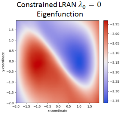
(a)

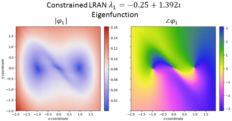
(b)

Figure 5: Unforced Duffing eigenfunctions learned using constrained LRAN

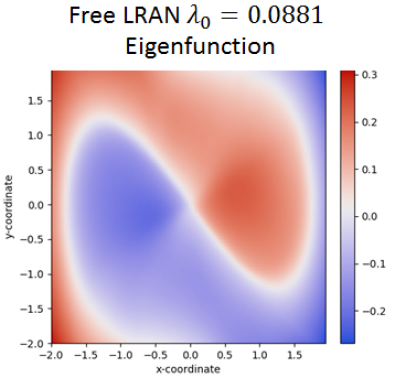
(a)

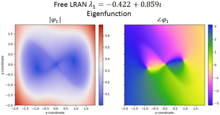
(b)

Figure 6: Unforced Duffing eigenfunctions learned using free LRAN

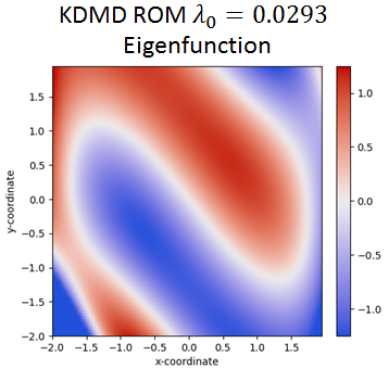
(a)

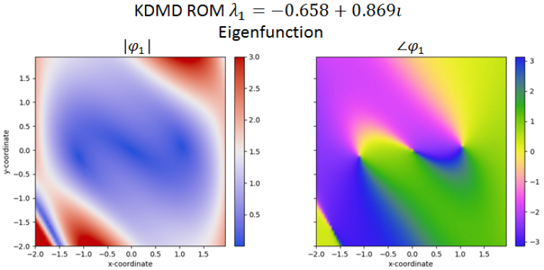
(b)

Figure 7: Unforced Duffing eigenfunctions found using KDMD balanced ROM

The other eigenfunction learned in each case parameterizes the basins of attraction and therefore is used to account for the dynamics in each basin. Each model appears to have learned a similar action-angle parameterization regardless of whether the eigenvalues were specified ahead of time. However, the constrained LRAN shows the best agreement with the true fixed point locations at $x=\pm 1$ where $\left|\varphi_{1}\right|\rightarrow 0$. The mean square relative prediction error was evaluated for each model by making predictions on the testing data set at various times in the future. The results plotted in Fig. 8 show that the free LRAN has by far the lowest prediction error likely due to the lack of constraints on the functions it could learn. It is surprising however, that nonlinear reconstruction hurt the performance of the KDMD reduced order model. This illustrates a potential difficulty with this method since the nonlinear part of the reconstruction is prone to over-fit without sufficient regularization.

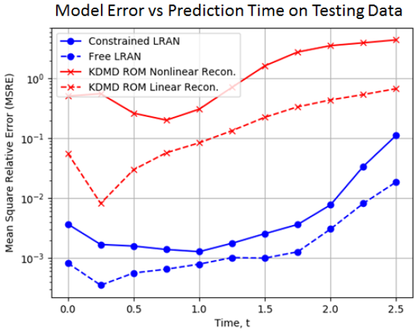
Figure 8: Unforced Duffing testing data mean square relative prediction errors for each model plotted against the prediction time

6.2 Cylinder wake

The next example we consider is the formation of a Kármán vortex sheet downstream of a cylinder in a fluid flow. This problem was chosen since the data has low intrinsic dimensionality due to the simple flow structure but is embedded in high-dimensional snapshots. We are interested in whether the proposed techniques can be used to discover very low dimensional models that accurately predict the dynamics over many time steps. We consider the growth of instabilities near an unstable base flow shown in Fig. 9a at Reynold number $Re=60$ all the way until a stable limit cycle shown in Fig. 9b is reached. The models will have to learn to make predictions over a range of unsteady flow conditions from the unstable equilibrium to the stable limit cycle.

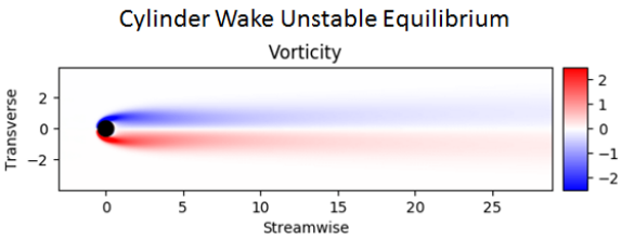
(a)

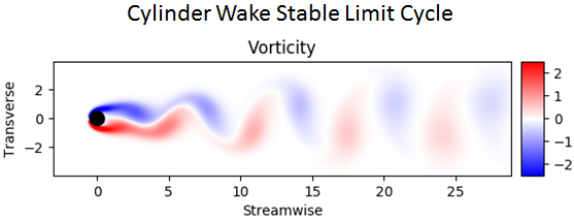
(b)

Figure 9: Example cylinder wake flow snapshots at the unstable equilibrium and on the stable limit cycle

The raw data consisted of $2000$ simulated snapshots of the velocity field taken at time intervals $0.2D/U_{\infty}$, where $D$ is the cylinder diameter and $U_{\infty}$ is the free-stream velocity. These data were split into $M_{\mbox{train}}=1000$ training, $M_{\mbox{eval}}=500$ evaluation, and $M_{\mbox{test}}=500$ testing data points. Odd numbered points $\Delta t=0.4D/U_{\infty}$ apart were used for training. The remaining $1000$ points were divided again into even and odd numbered points $2\Delta t=0.8D/U_{\infty}$ apart for evaluation and testing. This enabled training, evaluation, and testing on long data sequences while retaining coverage over the complete trajectory. The continuous-time eigenvalues are found from the discrete-time eigenvalues according to $\lambda=\log(\mu)/\Delta t=\log(\mu)U_{\infty}/(0.4D)$.

The raw data was projected onto its $200$ most energetic POD modes which captured essentially all of the energy in order to reduce the cost of storage and training. $400$-dimensional time delay embedded snapshots were formed from the state at time $t$ and $t+\Delta t$. A $5$th-order LRAN model and the 5th-order KDMD reduced order model were trained using the hyperparameters in Tables 3 and 4. In Fig. 10a, many of the discrete-time eigenvalues given by the over-specified KDMD model have approximately neutral stability with some being slightly unstable. However, the finite horizon formulation for balanced truncation allows us to learn the most dynamically salient eigenfunctions over a given length of time, in this case $\mathcal{T}=20$ steps or $8.0D/U_{\infty}$. We see in Fig. 10b that three of the eigenvalues learned by the two models are in close agreement and all are approximately neutrally stable.

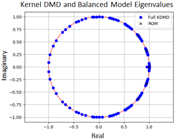
(a)

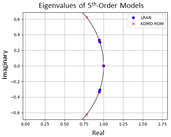
(b)

Figure 10: Discrete-time Koopman eigenvalues approximated by the KDMD ROM and the LRAN

A side-by-side comparison of the Koopman modes gives some insight into the flow structures whose dynamics the Koopman eigenvalues describe. We notice right away that the Koopman modes in Fig. 12b corresponding to continuous-time eigenvalue $\lambda_{1}$ are very similar for both models and indicate the pattern of vortex shedding downstream. This makes sense since a single frequency and mode will account for most of the amplitude as the limit cycle is approached. Evidently both models discover these limiting periodic dynamics. For the KDMD ROM, $\lambda_{2}$ is almost exactly the higher harmonic $2*\lambda_{1}$. The corresponding Koopman mode in Fig. 13b also reflects smaller flow structures which oscillate at twice the frequency of $\lambda_{1}$. Interestingly, the LRAN does not learn the same second eigenvalue as the KDMD ROM. The LRAN continuous-time eigenvalue $\lambda_{2}$ is very close to $\lambda_{1}$ which suggest that these frequencies might team up to produce the low-frequency $\lambda_{1}-\lambda_{2}$. The second LRAN Koopman mode in Fig. 13b also bears qualitative resemblance to the first Koopman mode in Fig. 12b, but with a slightly narrower pattern in the y-direction. The LRAN may be using the information at these frequencies to capture some of the slower transition process from the unstable fixed point to the limit cycle. The Koopman modes corresponding to $\lambda_{0}=0$ are also qualitatively different indicating that the LRAN and KDMD ROM are extracting different constant features from the data. We must be careful in our interpretation, however, since the LRAN’s koopman modes are only a least squares approximations to the nonlinear reconstruction process performed by the decoder.

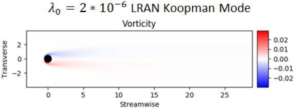
(a)

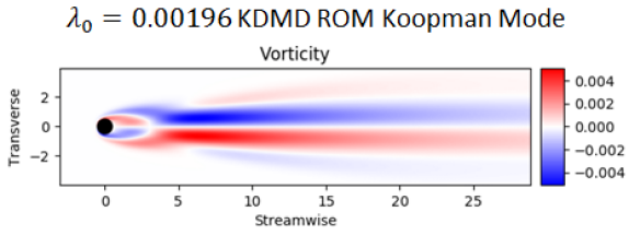
(b)

Figure 11: LRAN and KDMD ROM Koopman modes associated with $\lambda_{0}\approx 0$

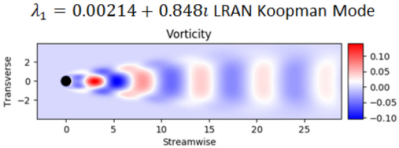
(a)

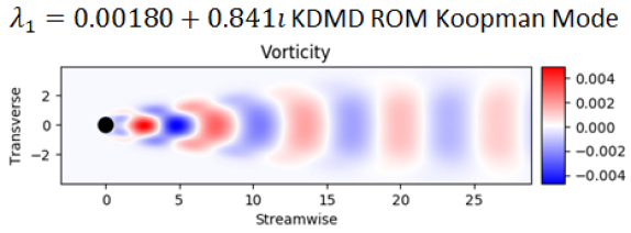
(b)

Figure 12: LRAN and KDMD ROM Koopman modes associated with $\lambda_{1}\approx 0.002+0.845\imath$

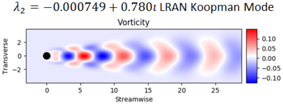
(a)

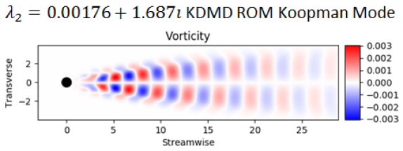
(b)

Figure 13: LRAN and KDMD ROM Koopman modes associated with $\lambda_{2}$ which differs greatly between the models

Plotting the model prediction error Fig. 14 shows that the linear reconstructions using both models have comparable performance with errors growing slowly over time. Therefore, the choice of the second Koopman mode does not seem to play a large role in the reconstruction process. However, when the nonlinear decoder is used to reconstruct the LRAN predictions, the mean relative error is roughly an order of magnitude smaller than the nonlinearly reconstructed KDMD ROM over many time steps. The LRAN has evidently learned an advantageous nonlinear transformation for reconstructing the data using the features evolving according to $\lambda_{2}$. The second Koopman mode reflects a linear approximation of this nonlinear transformation in the least squares sense.

Another remark is that nonlinear reconstruction using the KDMD ROM did significantly improve the accuracy in this example. This indicates that many of the complex variations in the data are really enslaved to a small number of modes. This makes sense since the dynamics are periodic on the limit cycle. Finally, it is worth mentioning that the prediction accuracy was achieved on average over all portions of the trajectory from the unstable equilibrium to the limit cycle. Both models therefore have demonstrated predictive accuracy and validity over a wide range of qualitatively different flow conditions. The nonlinearly reconstructed LRAN achieves a constant low prediction error over the entire time interval used for training $\mathcal{T}\Delta t=8.0D/U_{\infty}$. The error only begins to grow outside the interval used for training. The high prediction accuracy could likely be extended by training on longer data sequences.

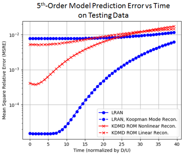
Figure 14: Cylinder wake testing data mean square relative prediction errors for each model plotted against the prediction time

6.3 Kuramoto-Sivashinsky equation

We now move on to test our new techniques on a very challenging problem — the Kuramoto-Sivashinsky equation in a parameter regime just beyond the onset of chaos. Since any chaotic dynamical system is mixing, it only has trivial Koopman eigenfunctions on its attractor(s). We therefore cannot expect our model to accurately reflect the dynamics of the real system. Rather, we aim to make predictions using very low-dimensional models that are accurate over short times and plausible over longer times.

The data was generated by performing direct numerical simulations of the Kuramoto-Sivashinsky equation,

(56) $$u_{t}+u_{xx}+u_{xxxx}+uu_{x}=0,\qquad x\in[0,L],$$

using a semi-implicit Fourier pseudo-spectral method. The length $L=8\pi$ was chosen where the equation first begins to exhibit chaotic dynamics [9]. $128$ Fourier modes were used to resolve all of the dissipative scales. Each data set: training, evaluation, and test, consisted of $20$ simulations from different initial conditions each with $500$ recorded states spaced by $\Delta t=1.0$. Snapshots consisted of time delay embedded states at $t$ and $t+\Delta t$. The initial conditions were formed by suppling Gaussian random perturbations to the coefficients on the $3$ linearly unstable Fourier modes $0<2\pi k/L<1\Longrightarrow k=1,2,3$.

An LRAN as well as a KDMD balanced ROM were trained to make predictions over a time horizon $\mathcal{T}=5$ steps using only $d=16$ dimensional models. Model parameters are given in Tables 5 and 6. The learned approximate Koopman eigenvalues are plotted in Fig. 15b. We notice that there are some slightly unstable eigenvalues, which makes sense since there are certainly unstable modes including the three linearly unstable Fourier modes. Additionally, Fig. 15b shows that some of the eigenvalues with large magnitude learned by the LRAN and the KDMD ROM are in near agreement.

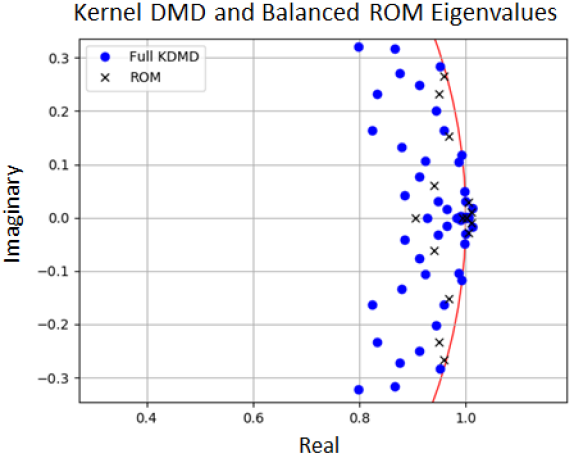
(a)

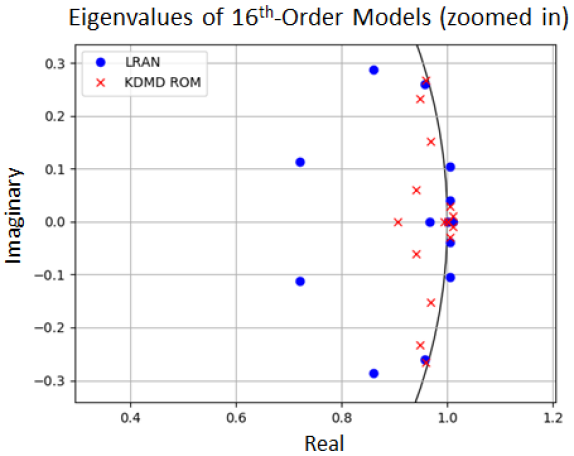
(b)

Figure 15: Discrete-time Koopman eigenvalues for the Kuramoto-Sivashinksy equation approximated by the KDMD ROM and the LRAN

The plot of mean square relative prediction error on the testing data set Fig. 16 indicates that our addition of nonlinear reconstruction from the low dimensional KDMD ROM state does not change the accuracy of the reconstruction. The performance of the KDMD ROM and the LRAN are comparable with the LRAN showing a modest reduction in error over all prediction times. It is interesting to note that the LRAN does not produce accurate reconstructions using the regression-based Koopman modes. In this example, the LRAN’s nonlinear decoder is essential for the reconstruction process. Evidently, the dictionary functions learned by the encoder require nonlinearity to reconstruct the state. Again, both models are most accurate over the specified time horizon $\mathcal{T}=5$ used for training.

Plotting some examples in Fig. 17b of ground truth and predicted test data sequences illustrates the behavior of the models. These examples show that both the LRAN and the KDMD ROM make quantitatively accurate short term predictions. While the predictions after $t\approx 5$ lose their accuracy as one would expect when trying to make linear approximations of chaotic dynamics, they remain qualitatively plausible. The LRAN model in particular is able to model and predict grouping and merging events between traveling waves in the solution. For example in Fig. 17a the LRAN successfully predicts the merging of two wave crests (in red) taking place between $t=2$ and $t=5$. The LRAN also predicts the meeting of a peak and trough in Fig. 17b at $t=5$. These results are encouraging considering the substantial reduction in dimensionality from a time delay embedded state of dimension $256$ to a $16$-dimensional encoded state having linear time evolution.

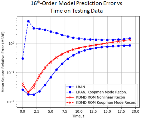
Figure 16: Kuramoto-Sivashinsky testing data mean square relative prediction errors for each model plotted against the prediction time

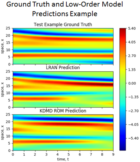
(a)

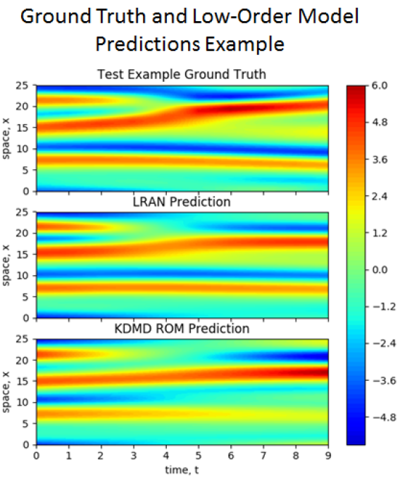
(b)

Figure 17: LRAN and KDMD ROM model predictions on Kuramoto-Sivashinsky test data examples

7 Conclusions

We have illustrated some fundamental challenges with EDMD, in particular highlighting the trade-off between rich dictionaries and over-fitting. The use of adaptive, low-dimensional dictionaries avoids the over-fitting problem while retaining enough capacity to represent Koopman eigenfunctions of complicated systems. This motivates the use of neural networks to learn sets of dictionary observables that are well-adapted to the given problems. By relaxing the constraint that the models must produce linear reconstructions of the state via the Koopman modes, we introduce a decoder neural network enabling the formation of very low-order models utilizing richer observables. Finally, by combining the neural network architecture that is essentially an autoencoder with linear recurrence, the LRAN learns features that are dynamically important rather than just energetic (i.e., large in norm).

Discovering a small set of dynamically important features or states is also the idea behind balanced model reduction. This led us to investigate the identification of low-dimensional models by balanced truncation of over-specified EDMD models, and in particular, KDMD models. Nonlinear reconstruction using a partially linear multi-kernel method was investigated for improving the reconstruction accuracy of the KDMD ROMs from very low-dimensional spaces. Our examples show that in some cases like the cylinder wake example, it can greatly improve the accuracy. We think this is because the data is intrinsically low-dimensional, but curves in such a way as to extend in many dimensions of the embedding space. The limiting case of the cylinder flow is an extreme example where the data becomes one-dimensional on the limit cycle. In some other cases, however, nonlinear reconstruction does not help, is sensitive to parameter choices, or decreases the accuracy due to over-fitting.

Our numerical examples indicate that unfolding the linear recurrence for many steps can improve the accuracy of LRAN predictions especially within the time horizon used during training. This is observed in the error versus prediction time plots in our examples: the error remains low and relatively flat for predictions made inside the training time horizon $\mathcal{T}$. The error then grows for predictions exceeding this length of time. However, for more complicated systems like the Kuramoto-Sivashinsky equation, one cannot unfold the network for too many steps before additional dimensions must be added to retain accuracy of the linear model approximation over time. These observations are also approximately true of the finite-horizon BPOD formulation used to create approximate balanced truncations of KDMD models. One additional consideration in forming balanced reduced-order models from finite-horizon impulse responses of over-specified systems is the problem of spurious eigenvalues whose associated modes only become significant for approximations as $t\rightarrow\infty$. The use of carefully chosen finite time horizons allows us to pick features which are the most relevant (observable and excitable) over any time span of interest.

The main drawback of the balanced reduced-order KDMD models becomes evident when making predictions on new evaluation and testing examples. While the LRAN has a high “up-front” cost to train — typically requiring hundreds of thousands of iterations — the cost of evaluating a new example is almost negligible and so very many predictions can be made quickly. On the other hand, every new example whose dynamics we want to predict using the KDMD reduced order model must still have its inner product evaluated with every training data point. Pruning methods like those developed for multi-output least squares support vector machines (LS-SVMs) will be needed to reduce the number of kernel evaluations before KDMD reduced order models can be considered practical for the purpose of predicting dynamics. The same will need to be done for kernel-based nonlinear reconstruction methods.

We conclude by discussing some exciting directions for future work on LRANs. The story certainly does not end with using them to learn linear encoded state dynamics and approximations of the Koopman eigenfunctions. The idea of establishing a possibly complicated transformation into and out of a space where the dynamics are simple is an underlying theme of this work. Human understanding seems to at least partly reside in finding isomorphism. If we can establish that a seemingly complicated system is topologically conjugate to a simple system, it doesn’t really matter what the transformation is as long as we can compute it. In this vein, the LRAN architecture is perfectly suited to learning the complicated transformations into and out of a space where the dynamics equations have a simple normal form. For example, this could be accomplished by learning coefficients on homogeneous polynomials of varying degree in addition to a matrix for updating the encoded state. One could also include learned parameter dependencies in order to study bifurcation behavior. Furthermore, any kind of symmetry could be imposed through either the normal form itself or through the neural network’s topology. For example, convolutional neural networks can be used in cases where the system is statistically stationary in a spatial coordinate.

Introduction of control terms to the dynamics of the encoded state is another interesting direction for inquiry. In some cases it might be possible to introduce a second autoencoder to perform a state-dependent encoding and decoding of the control inputs at each time step. Depending on the form that the inputs take in the evolution of the encoded state, it may be possible to apply a range of techniques from modern state-space control to nonlinear optimal control or even reinforcement learning-based control with policy and value functions parameterized by neural networks.

Another natural question is how the LRAN framework can be adapted to handle stochastic dynamics and uncertainty. Recent work in the development of structured inference networks for nonlinear stochastic models [12] may offer a promising approach. The low-dimensional dynamics and reconstruction process could be generalized to nonlinear stochastic processes for generating full state trajectories. Since the inference problem for such nonlinear systems is intractable, the encoder becomes a (bi-directional) recurrent neural network for performing approximate inference on the latent state given our data in analogy with Kalman smoothing. In this manner, many plausible outputs can be generated to estimate the distribution over state trajectories in addition to an inference distribution for quantifying uncertainty about the low-dimensional latent state.

Furthermore, with the above formulation of generative autoencoder networks for dynamics, it might be possible to employ adversarial training [8] in a similar manner to the adversarial autoencoder [17]. Training the generative network used for reconstruction against a discriminator network will encourage the generator to produce more plausible details like turbulent eddies in fluid flows which are not easily distinguished from the real thing.

Appendix A Hyperparameters used to train models

The same hyperparameters in Table 1 were used to train the constrained and free LRANs in the unforced Duffing equation example.

Table 1: Constrained LRAN hyperparameters for unforced Duffing example

Parameter	Value(s)
Time-delays embedded in a snapshot	$1$
Encoder layer widths (left to right)	$2$, $32$, $32$, $16$, $16$, $8$, $3$
Decoder layer widths (left to right)	$3$, $8$, $16$, $16$, $32$, $32$, $2$
Snapshot sequence length, $\mathcal{T}$	$10$
Weight decay rate, $\delta$	$0.8$
Relative weight on encoded state, $\beta$	$1.0$
Minibatch size	$50$ examples
Initial learning rate	$10^{-3}$
Geometric learning rate decay factor	$0.01$ per $4*10^{5}$ steps
Number of training steps	$4*10^{5}$

Table 2 summarizes the hyperparameters used to train the KDMD Reduced Order Model for the unforced Duffing example.

Table 2: KDMD ROM hyperparameters for unforced Duffing example

Parameter	Value(s)
Time-delays embedded in a snapshot	$1$
EDMD Dictionary kernel function	Gaussian RBF, $\sigma=10.0$
KDMD SVD rank, $r$	$27$
BPOD time horizon, $\mathcal{T}$	$10$
BPOD output projection rank	$2$ (no projection)
Balanced model order, $d$	$3$
Nonlinear reconstruction kernel function	Gaussian RBF, $\sigma=10.0$
Multi-kernel linear part truncation rank, $r_{1}$	$3$
Multi-kernel nonlinear part truncation rank, $r_{2}$	$8$
Multi-kernel regularization constant, $\gamma$	$10^{-4}$

The hyperparameters used to train the LRAN model on the cylinder wake data are given in Table 3.

Table 3: LRAN hyperparameters for cylinder wake example

Parameter	Value(s)
Time-delays embedded in a snapshot	$2$
Encoder layer widths (left to right)	$400$, $100$, $50$, $20$, $10$, $5$
Decoder layer widths (left to right)	$5$, $10$, $20$, $50$, $100$, $400$
Snapshot sequence length, $\mathcal{T}$	$20$
Weight decay rate, $\delta$	$0.95$
Relative weight on encoded state, $\beta$	$1.0$
Minibatch size	$50$ examples
Initial learning rate	$10^{-3}$
Geometric learning rate decay factor	$0.01$ per $2*10^{5}$ steps
Number of training steps	$2*10^{5}$

Table 4 summarizes the hyperparameters used to train the KDMD Reduced Order Model on the cylinder wake data.

Table 4: KDMD ROM hyperparameters for cylinder wake example

Parameter	Value(s)
Time-delays embedded in a snapshot	$2$
EDMD Dictionary kernel function	Gaussian RBF, $\sigma=10.0$
KDMD SVD rank, $r$	$100$
BPOD time horizon, $\mathcal{T}$	$20$
BPOD output projection rank	$100$
Balanced model order, $d$	$5$
Nonlinear reconstruction kernel function	Gaussian RBF, $\sigma=10.0$
Multi-kernel linear part truncation rank, $r_{1}$	$5$
Multi-kernel nonlinear part truncation rank, $r_{2}$	$15$
Multi-kernel regularization constant, $\gamma$	$10^{-8}$

Table 5 lists the hyperparameters used to train the LRAN model on the Kuramoto-Sivashinsky equation example.

Table 5: LRAN hyperparameters for Kuramoto-Sivashinsky example

Parameter	Value(s)
Time-delays embedded in a snapshot	$2$
Encoder layer widths (left to right)	$256$, $32$, $32$, $16$, $16$
Decoder layer widths (left to right)	$16$, $16$, $32$, $32$, $256$
Snapshot sequence length, $\mathcal{T}$	$5$
Weight decay rate, $\delta$	$0.9$
Relative weight on encoded state, $\beta$	$1.0$
Minibatch size	$50$ examples
Initial learning rate	$10^{-3}$
Geometric learning rate decay factor	$0.1$ per $2*10^{5}$ steps
Number of training steps	$4*10^{5}$

Table 6 summarizes the hyperparameters used to train the KDMD Reduced Order Model on the Kuramoto-Sivashinsky equation example data.

Table 6: KDMD ROM hyperparameters for Kuramoto-Sivashinsky example

Parameter	Value(s)
Time-delays embedded in a snapshot	$2$
EDMD Dictionary kernel function	Gaussian RBF, $\sigma=10.0$
KDMD SVD rank, $r$	$60$
BPOD time horizon, $\mathcal{T}$	$5$
BPOD output projection rank	$60$
Balanced model order, $d$	$16$
Nonlinear reconstruction kernel function	Gaussian RBF, $\sigma=100.0$
Multi-kernel linear part truncation rank, $r_{1}$	$16$
Multi-kernel nonlinear part truncation rank, $r_{2}$	$60$
Multi-kernel regularization constant, $\gamma$	$10^{-7}$

References

- [1] S. L. Brunton, J. L. Proctor, and J. N. Kutz, Discovering governing equations from data by sparse identification of nonlinear dynamical systems, Proceedings of the National Academy of Sciences of the United States of America, 113 (2016), pp. 3932–7, https://doi.org/10.1073/pnas.1517384113.
- [2] M. Budišić, R. Mohr, and I. Mezić, Applied koopmanism a, Chaos: An Interdisciplinary Journal of Nonlinear Science, 22 (2012), p. 047510.
- [3] D. Clevert, T. Unterthiner, and S. Hochreiter, Fast and accurate deep network learning by exponential linear units (elus), arXiv preprint arXiv:1511.07289, (2015).
- [4] G. E. Dullerud and F. Paganini, A Course in Robust Control Theory : a Convex Approach, Springer New York, 2000.
- [5] M. Espinoza, A. K. Suykens, and B. D. Moor, Kernel based partially linear models and nonlinear identification, IEEE Transactions on Automatic Control, 50 (2005), pp. 1602–6.
- [6] T. L. B. Flinois, A. S. Morgans, and P. J. Schmid, Projection-free approximate balanced truncation of large unstable systems, Physical Review E, 92 (2015), p. 023012.
- [7] I. Goodfellow, Y. Bengio, and A. Courville, Deep Learning, MIT Press, 2016.
- [8] I. Goodfellow, J. Pouget-Abadie, M. Mirza, B. Xu, D. Warde-Farley, S. Ozair, A. Courville, and Y. Bengio, Generative adversarial nets, in Advances in neural information processing systems, 2014, pp. 2672–2680.
- [9] P. Holmes, J. L. Lumley, G. Berkooz, and C. W. Rowley, Turbulence, Coherent Structures, Dynamical Systems and Symmetry, Cambridge University Press, 2012.
- [10] M. R. Jovanović, P. J. Schmid, and J. W. Nichols, Sparsity-promoting dynamic mode decomposition, Physics of Fluids, 26 (2014), p. 024103, https://doi.org/10.1063/1.4863670, http://aip.scitation.org/doi/10.1063/1.4863670.
- [11] B. O. Koopman, Hamiltonian systems and transformation in hilbert space, Proceedings of the National Academy of Sciences, 17 (1931), pp. 315–318.
- [12] R. G. Krishnan, U. Shalit, and D. Sontag, Structured inference networks for nonlinear state space models, in Proc. 31st AAAI Conference on Artificial Intelligence (AAAI-17), 2017.
- [13] Q. Li, F. Dietrich, E. M. Bollt, and I. G. Kevrekidis, Extended dynamic mode decomposition with dictionary learning: a data-driven adaptive spectral decomposition of the Koopman operator, arXiv preprint arXiv:1707.00225, (2017).
- [14] H. W. Lin, M. Tegmark, and D. Rolnick, Why does deep and cheap learning work so well?, arXiv preprint arXiv:1608.08225, (2016).
- [15] D. M. Luchtenburg and C. W. Rowley, Model reduction using snapshot-based realizations, Bulletin of the American Physical Society, Volume 56, Number 18 (2011), http://meetings.aps.org/Meeting/DFD11/Session/H19.4.
- [16] B. Lusch, J. N. Kutz, and S. L. Brunton, Deep learning for universal linear embeddings of nonlinear dynamics, arXiv preprint arXiv:1712.09707, (2017).
- [17] A. Makhzani, J. Shlens, N. Jaitly, I. Goodfellow, and B. Frey, Adversarial autoencoders, arXiv preprint arXiv:1511.05644, (2015).
- [18] L. Mescheder, S. Nowozin, and A. Geiger, Adversarial variational bayes: Unifying variational autoencoders and generative adversarial networks, arXiv preprint arXiv:1701.04722, (2017).
- [19] I. Mezić, Spectral properties of dynamical systems, model reduction and decompositions, Nonlinear Dynamics, 41 (2005), pp. 309–325, https://doi.org/10.1007/s11071-005-2824-x, http://link.springer.com/10.1007/s11071-005-2824-x.
- [20] I. Mezić, Koopman operator spectrum and data analysis, arXiv preprint arXiv:1702.07597, (2017).
- [21] B. Moore, Principal component analysis in linear systems: Controllability, observability, and model reduction, IEEE Transactions on Automatic Control, 26 (1981), pp. 17–32, https://doi.org/10.1109/TAC.1981.1102568.
- [22] W. Peng and Y. Ai-Jun, Improved pruning algorithm using quadratic renyi entropy for ls-svm modeling, in 24th Chinese Control and Decision Conference (CCDC), IEEE, 2012, pp. 3471–3474.
- [23] D. Rolnick and M. Tegmark, The power of deeper networks for expressing natural functions, arXiv preprint arXiv:1705.05502, (2017).
- [24] C. W. Rowley, Model reduction for fluids, using balanced proper orthogonal decomposition, International Journal of Bifurcation and Chaos, 15 (2005), pp. 997–1013.
- [25] C. W. Rowley, Data-driven methods for identifying nonlinear models of fluid flows, 2017. Presented at the Kavli Institute for Theoretical Physics, University of California, Santa Barbara.
- [26] C. W. Rowley and S. T. Dawson, Model reduction for flow analysis and control, Annual Review of Fluid Mechanics, 49 (2017), pp. 387–417, https://doi.org/10.1146/annurev-fluid-010816-060042, http://www.annualreviews.org/doi/10.1146/annurev-fluid-010816-060042.
- [27] C. W. Rowley, I. Mezić, S. Bagheri, P. Schlatter, and D. S. Henningson, Spectral analysis of nonlinear flows, Journal of Fluid Mechanics, 641 (2009), p. 115, https://doi.org/10.1017/S0022112009992059, http://www.journals.cambridge.org/abstract{_}S0022112009992059.
- [28] P. J. Schmid, Dynamic mode decomposition of numerical and experimental data, Journal of Fluid Mechanics, 656 (2010), pp. 5–28, https://doi.org/10.1017/S0022112010001217, http://www.journals.cambridge.org/abstract{_}S0022112010001217.
- [29] P. J. Schmid and D. S. Henningson, Stability and Transition in Shear Flows, vol. 142 of Applied Mathematical Sciences, Springer Verlag, 2001.
- [30] N. Takeishi, Y. Kawahara, and T. Yairi, Learning koopman invariant subspaces for dynamic mode decomposition, in Advances in Neural Information Processing Systems, 2017, pp. 1130–1140.
- [31] S. Tao, D. Chen, and W. Zhao, Fast pruning for multi-output ls-svm and its application to chemical pattern classification, Chemometrics and Intelligent Laboratory Systems, 96 (2009), pp. 63–69.
- [32] N. Watters, D. Zoran, T. Weber, P. Battaglia, R. Pascanu, and A. Tacchetti, Visual interaction networks: Learning a physics simulator from video, in Advances in Neural Information Processing Systems, 2017, pp. 4542–4550.
- [33] M. O. Williams, I. G. Kevrekidis, and C. W. Rowley, A data-driven approximation of the Koopman operator: Extending dynamic mode decomposition, Journal of Nonlinear Science, 25 (2015), pp. 1307–1346, https://doi.org/10.1007/s00332-015-9258-5, http://link.springer.com/10.1007/s00332-015-9258-5.
- [34] M. O. Williams, C. W. Rowley, and I. G. Kevrekidis, A kernel-based method for data-driven Koopman spectral analysis, Journal of Computational Dynamics, 2 (2016), pp. 247–265, https://doi.org/10.3934/jcd.2015005.
- [35] A. Wynn, D. S. Pearson, B. Ganapathisubramani, and P. J. Goulart, Optimal mode decomposition for unsteady flows, Journal of Fluid Mechanics, 733 (2013), pp. 473–503, https://doi.org/10.1017/jfm.2013.426, http://www.journals.cambridge.org/abstract{_}S0022112013004266.
- [36] Y.-L. Xu and D.-R. Chen, Partially-linear least-squares regularized regression for system identification, IEEE Transactions on Automatic Control, 54 (2009), pp. 2637–41.
- [37] E. Yeung, S. Kundu, and N. Hodas, Learning deep neural network representations for Koopman operators of nonlinear dynamical systems, arXiv preprint arXiv:1708.06850, (2017).
- [38] K. Zhou, G. Salomon, and E. Wu, Balanced realization and model reduction for unstable systems, International Journal of Robust and Nonlinear Control, 9 (1999), pp. 183–198, https://doi.org/10.1002/(SICI)1099-1239(199903)9:3<183::AID-RNC399>3.0.CO;2-E.