On construction of transmutation operators for perturbed Bessel equations

Abstract

A representation for the kernel of the transmutation operator relating the perturbed Bessel equation with the unperturbed one is obtained in the form of a functional series with coefficients calculated by a recurrent integration procedure. New properties of the transmutation kernel are established. A new representation of the regular solution of the perturbed Bessel equation is given presenting a remarkable feature of uniform error bound with respect to the spectral parameter for partial sums of the series. A numerical illustration of application to the solution of Dirichlet spectral problems is presented.

1 Introduction

In [1] it was proved that a regular solution of the perturbed Bessel equation

$$-u^{\prime\prime}+\left(\frac{l(l+1)}{x^{2}}+q(x)\right)u=\omega^{2}u,\quad x\in(0,b],$$ (1.1)

where $q\in C[0,b]$, $l\geq-\frac{1}{2}$, for all $\omega\in\mathbb{C}$ can be obtained from a regular solution of the unperturbed Bessel equation

$$-y^{\prime\prime}+\frac{l(l+1)}{x^{2}}y=\omega^{2}y$$ (1.2)

with the aid of a transmutation (transformation) operator in the form of a Volterra integral operator,

$$u(\omega,x)=T[y(\omega,x)]=y(\omega,x)+\int\limits_{0}^{x}K(x,t)y(\omega,t)dt.$$ (1.3)

Here the kernel $K$ is $\omega$-independent continuous function with respect to both arguments satisfying the Goursat condition

$$K(x,x)=\frac{1}{2}\int\limits_{0}^{x}q(s)\,ds.$$ (1.4)

A regular solution of (1.2) can be chosen in the form

$$y(\omega,x)=\sqrt{x}J_{l+\frac{1}{2}}(\omega x)$$

where $J_{\nu}$ stands for the Bessel function of the first kind and of order $\nu$. The transmutation operator (1.3) is a fundamental object in the theory of inverse problems related to (1.1) and has been studied in a number of publications (see, e.g., [2], [3], [4], [5], [6], [7], [8]).

Up to now apart from a successive approximation procedure used in [1], [4] for proving the existence of $K$ and a series representation proposed in [3] requiring the potential to possess holomorphic extension onto the disk of radius $2xe\sqrt{1+|2l|}$, no other construction of the transmutation kernel $K$ has been proposed. In this relation we mention the recent work [9] where $K$ was approximated by a special system of functions called generalized wave polynomials.

In the present paper we obtain an exact representation of the kernel $K$ in the form of a functional series whose coefficients are calculated following a simple recurrent integration procedure. The representation has an especially simple and attractive form in the case when $l$ is a natural number. It revealed some new properties of the kernel $K$.

The representation is obtained with the aid of a recent result from [10] where a Fourier-Legendre series expansion was derived for a certain kernel $R$ related to the kernel $K$. Here with the aid of an Erdelyi-Kober fractional derivative we express $K$ in terms of $R$ which leads to a series representation for the kernel $K$.

The obtained form of the kernel $K$ is appropriate both for studying the exact solution as well as the properties of the kernel itself, and for numerical applications.

In Section 2 some previous results are recalled and an expression for the kernel $K$ in terms of $R$ is derived. In Section 3 a functional series representation for $K$ is obtained in the case of integer parameter $l$. Its convergence properties are studied.

In Section 4 the obtained representation of the kernel $K$ is used for deriving a new representation for regular solution of the perturbed Bessel equation enjoying the uniform ($\omega$-independent) approximation property (Theorem 4). Since the regular solution $u(\omega,x)$ in this representation is the image of $\sqrt{\omega x}J_{l+1/2}(\omega x)$ under the action of the transmutation operator $T$, $u(\omega,x)$ does not decay to zero as $\omega\to\infty$. Hence partial sums of the representation provide good approximation even for arbitrarily large values of the spectral parameter $\omega$. This is an advantage in comparison with the representation from [10] derived for a regular solution decaying as $\omega^{-l-1}$ when $\omega\to\infty$, making the approximation by partial sums useful for reasonably small values of $\omega$ only.

In Section 5 a functional series representation for the kernel $K$ is obtained in the case of a noninteger $l$. Section 6 contains some numerical illustrations confirming the validity of the presented results.

2 A representation of $K(x,t)$ using an Erdelyi-Kober operator

In this section, with the aid of a result from [10] we obtain a representation of the kernel $K(x,t)$ in terms of an Erdelyi-Kober fractional derivative applied to a certain Fourier-Legendre series. Two transmutation operators are used, a modified Poisson transmutation operator and the transmutation operator (1.3).

2.1 The modified Poisson transmutation operator

The Poisson transmutation operator examined in [11] and [7] is adapted to work with the singular differential Bessel operator $B_{\gamma}=\frac{d^{2}}{dx^{2}}+\frac{\gamma}{x}\frac{d}{dx}$, where $\gamma>0$. We will use a slightly modified Poisson operator defined on $C([0,b])$ of the form (see [10] and [9])

$$Y_{l,x}f(x)=\frac{x^{-l}}{2^{l+\frac{1}{2}}\Gamma\left(l+\frac{3}{2}\right)}\int\limits_{0}^{x}(x^{2}-s^{2})^{l}f(s)ds,\quad l\geq-\frac{1}{2}.$$ (2.1)

The following equality is valid

$$Y_{l,x}[\cos{\omega x}]=\frac{\sqrt{\pi}\Gamma(l+1)}{2\omega^{l+1}\Gamma\left(l+\frac{3}{2}\right)}\,\sqrt{\omega x}\,J_{l+\frac{1}{2}}(\omega x).$$

Moreover, $Y_{l,x}$ is an intertwining operator for $\frac{d^{2}}{dx^{2}}$ and $\frac{d^{2}}{dx^{2}}-\frac{l(l+1)}{x^{2}}$ in the following sense. If $v\in C^{2}[0,b]$ and $v^{\prime}(0)=0$ then

$$Y_{l,x}\frac{d^{2}v}{dx^{2}}=\left(\frac{d^{2}}{dx^{2}}-\frac{l(l+1)}{x^{2}}\right)Y_{l,x}v.$$

In particular, the regular solution of equation (1.2) satisfying the asymptotic relations $y_{0}(x){\sim}x^{l+1}$ and $y_{0}^{\prime}(x){\sim}(l{+}1)x^{l}$, when $x\rightarrow 0$ can be written in the form

$$y(\omega,x)=\frac{2^{l+\frac{3}{2}}\Gamma^{2}\left(l+\frac{3}{2}\right)}{\sqrt{\pi}\Gamma(l+1)}Y_{l,x}[\cos(\omega x)]=\Gamma\left(l+\frac{3}{2}\right)2^{l+\frac{1}{2}}\omega^{-l-\frac{1}{2}}\sqrt{x}J_{l+\frac{1}{2}}(\omega x).$$ (2.2)

The composition of two transmutation operators (1.3) and (2.1) allows one to write a regular solution of (1.1) in the form (see [10])

$$u(\omega,x)=\frac{2^{l+\frac{1}{2}}\Gamma\left(l+\frac{3}{2}\right)}{\omega^{l+\frac{1}{2}}}\sqrt{x}\,J_{l+\frac{1}{2}}(\omega x)+\int\limits_{0}^{x}R(x,t)\cos{\omega t}dt,$$ (2.3)

where the kernel $R(x,t)$ is a sufficiently regular function which admits a convergent Fourier–Legendre series expansion presented in [10]. Namely,

$$R(x,t)=\sum\limits_{k=0}^{\infty}\frac{\beta_{k}(x)}{x}P_{2k}\left(\frac{t}{x}\right),$$ (2.4)

where $P_{m}(x)$ stands for the Legendre polynomial of order $m$, and the coefficients $\beta_{k}$ can be computed following a simple recurrent integration procedure [10].

2.2 A representation of $K(x,t)$ in terms of $R(x,t)$

Theorem 1.

Let $q\in C[0,b]$ be a complex-valued function. Then the following equality is valid

$$K(x,t)=\frac{\sqrt{\pi}}{\Gamma\left(l+\frac{3}{2}\right)}\frac{t^{l+1}}{\Gamma(n-l-1)}\left(-\frac{d}{2tdt}\right)^{n}\int\limits_{t}^{x}(s^{2}-t^{2})^{n-l-2}sR(x,s)ds,$$ (2.5)

here $n$ can be arbitrary integer satisfying $n>l+1$.

Proof. The following relation between the kernels $K$ and $R$ was obtained in [10, (3.10) and (3.12)]

$$\frac{2\Gamma\left(l+\frac{3}{2}\right)}{\sqrt{\pi}\Gamma(l+1)}\int\limits_{s}^{x}K(x,t)t^{-l}(t^{2}-s^{2})^{l}dt=R(x,s).$$ (2.6)

Let us invert this equality using an inverse Erdelyi-Kober operator. For $\alpha>0$ the left-sided Erdelyi-Kober operator is (see [12, (18.3)])

$$I_{x-;2,\eta}^{\alpha}f(s){=}\frac{2s^{\sigma\eta}}{\Gamma(\alpha)}\int\limits_{s}^{x}(t^{2}-s^{2})^{\alpha-1}t^{2(1-\alpha-\eta)-1}f(t)dt,$$ (2.7)

that means we can rewrite (2.6) as

$$\frac{\Gamma\left(l+\frac{3}{2}\right)}{\sqrt{\pi}}\,t^{l+1}\,I_{x-;2,-\frac{l+1}{2}}^{l+1}K(x,t)=R(x,t).$$ (2.8)

Now applying the inverse operator for (2.7) we obtain (2.5). ∎

3 Representation of $K(x,t)$ for $l=0,1,2,...$

The relation (2.5) together with the Fourier-Legendre series representations of $R$ in (2.4) lead to a Fourier-Jacobi series representation of the kernel $K$. It admits an especially simple form in the case of integer values of the parameter $l$.

Theorem 2.

Let $q\in C^{1}[0,b]$. For $l=0,1,2,...$ the following formula for the kernel of the transmutation operator (1.3) is valid

$$K(x,t)=\frac{\sqrt{\pi}t^{l+1}}{x^{2l+3}\Gamma\left(l+\frac{3}{2}\right)}\sum\limits_{m=0}^{\infty}\frac{(-1)^{m+l+1}\Gamma\left(m+2l+\frac{5}{2}\right)}{\Gamma\left(m+l+\frac{3}{2}\right)}\beta_{m+l+1}(x)P_{m}^{\left(l+\frac{1}{2},l+1\right)}\left(1-2\frac{t^{2}}{x^{2}}\right),$$ (3.1)

where $\,P_{m}^{\left(\alpha,\beta\right)}$ stands for a Jacobi polynomial and the coefficients $\beta_{k}$ are those from Subsection 2.1.

The series (3.1) converges absolutely for any $x\in(0,b]$ and $t\in(0,x)$ and converges uniformly with respect to $t$ on any segment $[\varepsilon,x-\varepsilon]\subset(0,x)$. Under the additional assumption that $q\in C^{2l+5}[0,b]$ the series (3.1) converges absolutely and uniformly with respect to $t$ on $[0,x]$.

Proof. For any nonnegative integer $l$ and $n>l+1$ we can rewrite formula (2.5) in the form

$$K(x,t)=\frac{(-1)^{l+1}\sqrt{\pi}}{\Gamma\left(l+\frac{3}{2}\right)}\frac{t^{l+1}}{\Gamma(n-l-1)}\left(\frac{d}{2tdt}\right)^{n}\int\limits_{x}^{t}(t^{2}-s^{2})^{n-l-2}sR(x,s)ds.$$ (3.2)

Choosing $n=l+2$ we obtain

$$K(x,t)=\frac{(-1)^{l+1}\sqrt{\pi}t^{l+1}}{\Gamma\left(l+\frac{3}{2}\right)}\left(\frac{d}{2tdt}\right)^{l+2}\int\limits_{x}^{t}sR(x,s)ds=\frac{(-1)^{l+1}\sqrt{\pi}t^{l+1}}{\Gamma\left(l+\frac{3}{2}\right)}\left(\frac{d}{2tdt}\right)^{l+1}R(x,t).\\$$ (3.3)

Substituting the series expansion (2.4) into (3.3) we get (we left the justification of the possibility of termwise differentiation of (2.4) to the end of the proof)

$$K(x,t)=\frac{(-1)^{l+1}\sqrt{\pi}t^{l+1}}{\Gamma\left(l+\frac{3}{2}\right)}\sum\limits_{k=0}^{\infty}\frac{\beta_{k}(x)}{x}\left(\frac{d}{2tdt}\right)^{l+1}P_{2k}\left(\frac{t}{x}\right).$$

Now we would like to calculate the derivatives

$$\left(\frac{d}{2tdt}\right)^{l+1}P_{2k}\left(\frac{t}{x}\right)=\left(\frac{d}{dt^{2}}\right)^{l+1}P_{2k}\left(\frac{t}{x}\right).$$

Note that by formula 8.911 from [13] the following equality is valid

$$\begin{split}P_{2k}\left(\frac{t}{x}\right)&=(-1)^{k}\frac{(2k-1)!!}{2^{k}k!}\,_{2}F_{1}\left(-k,k+\frac{1}{2};\frac{1}{2};\frac{t^{2}}{x^{2}}\right)=(-1)^{k}\frac{\left(\frac{1}{2}\right)_{k}}{k!}\,_{2}F_{1}\left(-k,k+\frac{1}{2};\frac{1}{2};\frac{t^{2}}{x^{2}}\right).\end{split}$$

Now application of formula 15.2.2 from [14],

$$\frac{d^{n}}{dz^{n}}F(a,b;c;z)=\frac{(a)_{n}(b)_{n}}{(c)_{n}}F(a+n,b+n;c+n;z)$$

leads to the relation

$$\left(\frac{d}{dt^{2}}\right)^{l+1}P_{2k}\left(\frac{t}{x}\right)=(-1)^{k}\frac{\left(\frac{1}{2}\right)_{k}}{k!}\frac{(-k)_{l+1}\left(k+\frac{1}{2}\right)_{l+1}}{x^{2l+2}\left(\frac{1}{2}\right)_{l+1}}\,_{2}F_{1}\left(l+1-k,k+l+\frac{3}{2};l+\frac{3}{2};\frac{t^{2}}{x^{2}}\right).$$

Taking into account that $(-k)_{l+1}=0$ when $l\geq k$ and $(-k)_{l+1}=(-1)^{l+1}\frac{k!}{\Gamma(k-l)}$ when $l<k$, we obtain

$$\left(\frac{d}{dt^{2}}\right)^{l+1}P_{2k}\left(\frac{t}{x}\right)=0$$

when $l\geq k$, and

$$\begin{split}\left(\frac{d}{2tdt}\right)^{l+1}P_{2k}\left(\frac{t}{x}\right)&=(-1)^{k+l+1}\frac{\left(\frac{1}{2}\right)_{k}\left(k+\frac{1}{2}\right)_{l+1}}{x^{2l+2}\Gamma(k-l)\left(\frac{1}{2}\right)_{l+1}}\,_{2}F_{1}\left(l+1-k,k+l+\frac{3}{2};l+\frac{3}{2};\frac{t^{2}}{x^{2}}\right)\\ &=(-1)^{k+l+1}\frac{\Gamma\left(k+l+\frac{3}{2}\right)}{x^{2l+2}\Gamma(k-l)\Gamma\left(l+\frac{3}{2}\right)}\,_{2}F_{1}\left(l+1-k,k+l+\frac{3}{2};l+\frac{3}{2};\frac{t^{2}}{x^{2}}\right)\end{split}$$

when $l<k$. Thus,

$$\begin{split}K(x,t)&=\frac{\sqrt{\pi}t^{l+1}}{x^{2l+3}\Gamma\left(l+\frac{3}{2}\right)}\sum\limits_{k=l+1}^{\infty}(-1)^{k}\beta_{k}(x)\frac{\Gamma\left(k+l+\frac{3}{2}\right)}{\Gamma(k-l)\Gamma\left(l+\frac{3}{2}\right)}\,_{2}F_{1}\left(l+1-k,k+l+\frac{3}{2};l+\frac{3}{2};\frac{t^{2}}{x^{2}}\right).\\ &=\frac{\sqrt{\pi}t^{l+1}}{x^{2l+3}\Gamma\left(l+\frac{3}{2}\right)}\sum\limits_{m=0}^{\infty}(-1)^{m+l+1}\beta_{m+l+1}(x)\\ &\quad\times\frac{\Gamma\left(m+2l+\frac{5}{2}\right)}{\Gamma(m+1)\Gamma\left(l+\frac{3}{2}\right)}\,_{2}F_{1}\left(-m,m+2l+\frac{5}{2};l+\frac{3}{2};\frac{t^{2}}{x^{2}}\right).\end{split}$$ (3.4)

The series for $\,{}_{2}F_{1}(a,b;c;z)$ terminates if either $a$ or $b$ is a nonpositive integer, in which case the function reduces to a polynomial. In particular, according to [14, formula 15.4.6],

$$\,{}_{2}F_{1}(-m,m+\alpha+1+\beta;\alpha+1;x)=\frac{m!}{(\alpha+1)_{m}}P_{m}^{(\alpha,\beta)}(1-2x).$$ (3.5)

Substitution of (3.5) into (3.4) gives us (3.1).

Using the asymptotic formula [14, (6.1.40)] one can check that

$$\log\frac{\Gamma(m+2l+5/2)}{\Gamma(m+l+3/2)}=(l+1)\log(m+l+1)+O\left(\frac{1}{m+l+1}\right),\qquad m\to\infty.$$ (3.6)

Theorem 7.32.2 from [15] states that

$$\left|P_{m}^{(l+1/2,l+1)}(z)\right|\leq\frac{C_{\varepsilon}}{\sqrt{m}}$$ (3.7)

uniformly for $z\in[-1+\varepsilon,1-\varepsilon]$. And it was shown in [10, (4.15)] that for $q\in C^{1}[0,b]$

$$|\beta_{m+l+1}(x)|\leq\frac{cx^{l+3}}{(m+l)^{l+2}},\qquad m\geq 2.$$ (3.8)

Combining (3.6), (3.7) and (3.8) we obtain the absolute convergence of the series (3.1) for $x\in(0,b]$ and $t\in(0,x)$, uniform with respect to $t$ on any $[\varepsilon_{1},x-\varepsilon_{1}]$.

For the whole segment $[0,x]$ note that the Jacobi polynomials satisfy

$$|P_{m}^{(l+1/2,l+1)}(z)|\leq Cm^{l+1},\qquad z\in[-1,1],$$ (3.9)

see [15, Theorem 7.32.4], while for $q\in C^{2l+5}[0,b]$ the coefficients $\beta_{m+l+1}$ satisfy [10, (4.15)]

$$|\beta_{m+l+1}(x)|\leq\frac{c_{2}x^{2l+5}}{(m+l)^{2l+4}}.$$ (3.10)

Combining (3.6), (3.9) with (3.10) we obtain the uniform convergence with respect to $t$ on the whole segment $[0,x]$.

The possibility of termwise differentiation of the series (2.4) follows directly from the presented results. Namely, the expressions $\left(\frac{d}{2t\,dt}\right)^{j}R(x,t)$, $j\leq l+1$ lead to series similar to (3.1) but having $j$ instead of $l+1$, uniformly convergent with respect to $t$ on any segment $[\varepsilon,x-\varepsilon]$. ∎

Corollary 1.

Let $q\in C^{2l+5}[0,b]$. Using the formula

$$P_{n}^{{(\alpha,\beta)}}(-1)=(-1)^{n}{\binom{n+\beta}{n},}$$

from (3.1) and taking into account (1.4) we find the relation

$$\frac{1}{2}\int\limits_{0}^{x}q(s)\,ds=\frac{(-1)^{l+1}}{x^{l+2}}\frac{\sqrt{\pi}}{\Gamma\left(l+\frac{3}{2}\right)}\sum\limits_{m=0}^{\infty}\beta_{m+l+1}(x)\frac{\Gamma\left(m+2l+\frac{5}{2}\right)}{\Gamma\left(m+l+\frac{3}{2}\right)}{\binom{m+l+1}{m}}.$$ (3.11)

The representation (3.1) may be substituted termwise in (1.3) under less restrictive convergence assumption than the uniform convergence. Namely, $L_{1}[0,x]$ convergence with respect to $t$ is sufficient to apply the transmutation operator (1.3) with the integral kernel given by (3.1) to a bounded function. Let us rewrite the formula (3.1) as

$$K(x,t)=\frac{(-1)^{l+1}\sqrt{\pi}}{x^{2l+3}\Gamma\left(l+\frac{3}{2}\right)}\sum\limits_{m=0}^{\infty}\frac{(-1)^{m}\Gamma\left(m+2l+\frac{5}{2}\right)}{\Gamma\left(m+l+\frac{3}{2}\right)}\beta_{m+l+1}(x)t^{l+1}P_{m}^{\left(l+\frac{1}{2},l+1\right)}\left(1-2\frac{t^{2}}{x^{2}}\right).$$ (3.12)

The following proposition states the $L_{1}$ convergence of the series (3.12) under slightly relaxed requirement on the smoothness of the potential $q$.

Proposition 1.

Let $l\geq 1$. Under the condition $q\in C^{2l+1}[0,b]$ the series (3.12) converges for every fixed $x$ in $L_{1}[0,x]$ norm.

Proof. Consider

$$\begin{split}p_{m}:&=\int\limits_{0}^{x}t^{l+1}\left|P_{m}^{(l+1/2,l+1)}\left(1-2\frac{t^{2}}{x^{2}}\right)\right|\,dt=\frac{x^{l+2}}{2^{l/2+2}}\int\limits_{-1}^{1}(1-z)^{l/2}\left|P_{m}^{(l+1/2,l+1)}(z)\right|\,dz\\ &\leq\frac{x^{l+2}}{2^{l/2+2}}\int\limits_{0}^{1}(1-z)^{l/2}\left|P_{m}^{(l+1/2,l+1)}(z)\right|\,dz+\frac{x^{l+2}}{4}\int\limits_{0}^{1}\left|P_{m}^{(l+1,l+1/2)}(z)\right|\,dz.\end{split}$$ (3.13)

Theorem 7.34 from [15] states that

$$\int\limits_{0}^{1}(1-x)^{\mu}\left|P_{n}^{(\alpha,\beta)}(x)\right|\,dx\sim\begin{cases}n^{\alpha-2\mu-2},&\text{if }2\mu<\alpha-\frac{3}{2},\\ n^{-1/2},&\text{if }2\mu>\alpha-3/2,\end{cases}\qquad n\to\infty,$$

whenever $\alpha$, $\beta$, $\mu$ are real numbers greater than $-1$. Using this result to estimate both integrals in (3.13) we obtain that for some constant $C$ and all $m\geq 1$

$$p_{m}\leq Cx^{l+2}m^{l-1}.$$

Hence $L_{1}[0,x]$ norms of the functions $\frac{\Gamma(m+2l+5/2)}{\Gamma(m+l+3/2)}P_{m}^{(l+1/2,l+1)}(1-2\frac{t^{2}}{x^{2}})$ grow at most as $m^{2l}$, $m\to\infty$, and the estimate

$$|\beta_{m+l+1}(x)|\leq\frac{c_{3}x^{2l+3}}{(m+l)^{2l+2}},$$

valid (see [10, (4.150]) under the condition $q\in C^{2l+1}[0,b]$, is sufficient to assure the convergence of the series (3.1) in the $L_{1}[0,x]$ norm. ∎

Remark 1.

The smoothness requirements $q\in C^{2l+5}[0,b]$ in Theorem 2 and Corollary 1 and $q\in C^{2l+1}[0,b]$ in Proposition 1 may be excessive. However the minimal requirement $q\in C^{1}[0,b]$ may be insufficient in general neither for the representation (3.11) to converge, nor for (3.1) to converge in $L_{1}[0,x]$. Indeed, one can easily check that the factor $\frac{\Gamma\left(m+2l+5/2\right)}{\Gamma\left(m+l+3/2\right)}{\binom{m+l+1}{m}}$ grows as $(m+l+1)^{2l+2}$, $m\to\infty$ requiring the coefficients $\beta_{m}$ to decay faster than $m^{-2l-2}$ in order to fulfill at least the necessary convergence condition (terms of a series goes to zero as $m\to\infty$). Similarly, by slightly changing the reasoning in the proof of Proposition 1 one can see that the numbers $p_{m}$ grow as $m^{l-1}$, requiring the coefficients $\beta_{m}$ to decay faster than $m^{-2l}$ for the $L_{1}$ convergence of the series (3.1).

Numerical experiments similar to those from [10, Section 9.1] suggest that this may not happen. For the potential

$$q_{2}(x)=\begin{cases}1,&x\in[0,\pi/2],\\ 1+(x-\pi/2)^{2},&x\in[\pi/2,\pi],\end{cases}$$

having its second derivative bounded on $[0,\pi]$, and for $l=3$, the observed decay rate of the coefficients $\beta_{m}(x)$ was $Cm^{-7.5}$, $m\to\infty$, insufficient for the convergence of the series (3.11). While for $l=5$ the observed decay rate of the coefficients $\beta_{m}(x)$ was $Cm^{-9.5}$, $m\to\infty$, insufficient for the $L_{1}$ convergence of the series (3.1).

Corollary 2.

The integral of the power function multiplied by the kernel $K(x,t)$ has the form

$$\begin{split}\int\limits_{0}^{x}t^{\alpha}K(x,t)dt&=\frac{x^{\alpha-l-1}}{2\left(\frac{\alpha+l}{2}+1\right)}\frac{\sqrt{\pi}}{\Gamma^{2}\left(l+\frac{3}{2}\right)}\sum\limits_{m=0}^{\infty}(-1)^{m+l+1}\beta_{m+l+1}(x)\frac{\Gamma\left(m+2l+\frac{5}{2}\right)}{m!}\\ &\quad\times\,_{3}F_{2}\left({-}m,2l{+}m{+}\frac{5}{2},\frac{\alpha{+}l}{2}{+}1;l{+}\frac{3}{2},\frac{\alpha{+}l}{2}{+}2;1\right),\qquad\operatorname{Re}\alpha>-l-2.\end{split}$$ (3.14)

Proof. Due to (3.4), we have

$$\begin{split}\int\limits_{0}^{x}t^{\alpha}K(x,t)dt&=\frac{1}{x^{2l+3}}\frac{\sqrt{\pi}}{\Gamma\left(l+\frac{3}{2}\right)}\sum\limits_{m=0}^{\infty}(-1)^{m+l+1}\beta_{m+l+1}(x)\frac{\Gamma\left(m+2l+\frac{5}{2}\right)}{\Gamma\left(m+l+\frac{3}{2}\right)}\\ &\quad\times\int\limits_{0}^{x}t^{\alpha+l+1}P_{m}^{\left(l+\frac{1}{2},l+1\right)}\left(1-2\frac{t^{2}}{x^{2}}\right)dt.\end{split}$$ (3.15)

Consider the integral

$$\int\limits_{0}^{x}t^{\alpha+l+1}P_{m}^{\left(l+\frac{1}{2},l+1\right)}\left(1-2\frac{t^{2}}{x^{2}}\right)dt=2^{-2-\frac{\alpha+l}{2}}x^{\alpha+l+2}\int\limits_{-1}^{1}(1-z)^{\frac{\alpha+l}{2}}P_{m}^{\left(l+\frac{1}{2},l+1\right)}(z)dz.$$

Here we use the formula 16.4.3 from [16]

$$\begin{split}\int\limits_{-1}^{1}(1-x)^{\rho}(1+x)^{\sigma}P_{n}^{(\alpha,\beta)}(x)dx&=\frac{2^{\rho+\sigma+1}\Gamma(\rho+1)\Gamma(\sigma+1)}{\Gamma(\rho+\sigma+2)}\,\frac{\Gamma(n+\alpha+1)}{n!\Gamma(\alpha+1)}\\ &\quad\times\,_{3}F_{2}(-n,\alpha+\beta+n+1,\rho+1;\alpha+1,\rho+\sigma+2;1),\\ &\mathrm{Re}\,\rho>-1,\qquad\mathrm{Re}\,\sigma>-1.\end{split}$$

In particular, we have

$$\begin{split}\int\limits_{-1}^{1}(1-z)^{\frac{\alpha+l}{2}}P_{m}^{\left(l+\frac{1}{2},l+1\right)}(z)dz&=\frac{2^{\frac{\alpha+l}{2}+1}}{\left(\frac{\alpha+l}{2}+1\right)}\frac{\Gamma\left(m+l+\frac{3}{2}\right)}{m!\Gamma\left(l+\frac{3}{2}\right)}\\ &\quad\times\,_{3}F_{2}\left({-}m,2l{+}m{+}\frac{5}{2},\frac{\alpha{+}l}{2}{+}1;l{+}\frac{3}{2},\frac{\alpha{+}l}{2}{+}2;1\right).\end{split}$$ (3.16)

Substitution of (3.16) into (3.15) gives us (3.14). ∎

Remark 2.

In [18] the images of $x^{2k+l+1}$ under the action of the operator $T$ were obtained for any $l\geq-1/2$ and $k=0,1,2,\ldots$. In the case of integer $l$ they can be derived from (3.14). For example, one can see using (3.14) together with the equality [10, formula 9.1] $\sum\limits_{k=0}^{\infty}\beta_{k}(x)=0$ that for $\alpha=1$ and $l=0$ the following relation is valid

$$\int\limits_{0}^{x}tK(x,t)dt=\beta_{0}(x).$$

4 Representation of the regular solution for $l=1,2,\ldots$

Substituting (3.12) into (1.3) we obtain that the regular solution of (1.1) has the form

$$\begin{split}u(\omega,x)&=\sqrt{x}J_{l+1/2}(\omega x)+\frac{\sqrt{\pi}}{x^{2l+3}\Gamma(l+3/2)}\sum_{m=0}^{\infty}\frac{(-1)^{m+l+1}\Gamma(m+2l+5/2)}{\Gamma(m+l+3/2)}\beta_{m+l+1}(x)\\ &\quad\times\int\limits_{0}^{x}t^{l+3/2}J_{l+1/2}(\omega t)P_{m}^{(l+1/2,l+1)}\left(1-2\frac{t^{2}}{x^{2}}\right)\,dt.\end{split}$$

Consider the integrals

$$\mathcal{I}_{k,m}(\omega,x):=\int\limits_{0}^{x}t^{k+3/2}J_{k+1/2}(\omega t)P_{m}^{(k+1/2,k+1)}\left(1-2\frac{t^{2}}{x^{2}}\right)\,dt.$$

For $m=0$ the formula 1.8.1.3 from [17] gives

$$\mathcal{I}_{k,0}(\omega,x)=\frac{x^{k+3/2}}{\omega}J_{k+3/2}(\omega x).$$ (4.1)

Let $m>0$. Integrating by parts, taking into account (4.1) and noting that $\frac{d}{dx}P_{n}^{(\alpha,\beta)}(x)=\frac{1}{2}(n+\alpha+\beta+1)P_{n-1}^{(\alpha+1,\beta+1)}(x)$ we obtain that

$$\begin{split}\mathcal{I}_{k,m}(\omega,x)&=\left.\frac{t^{k+3/2}}{\omega}J_{k+3/2}(\omega t)P_{m}^{(k+1/2,k+1)}\left(1-2\frac{t^{2}}{x^{2}}\right)\right|_{t=0}^{x}\\ &\quad-\int\limits_{0}^{x}\frac{t^{k+3/2}}{\omega}J_{k+3/2}(\omega t)\cdot\frac{1}{2}(m+2k+5/2)P_{m-1}^{(k+3/2,k+2)}\left(1-2\frac{t^{2}}{x^{2}}\right)\cdot\left(-\frac{4t}{x^{2}}\right)\,dt\\ &=(-1)^{m}\binom{m+k+1}{m}\mathcal{I}_{k,0}(\omega,x)+\frac{2m+4k+5}{\omega x^{2}}\mathcal{I}_{k+1,m-1}(\omega,x).\end{split}$$

Hence we obtain the following result.

Theorem 3.

Let $q\in C^{2l+1}[0,b]$. Then the regular solution $u(\omega,x)$ of equation (1.1) satisfying the asymptotics $u(\omega,x)\sim\frac{(\omega x)^{l+1}}{2^{l+1/2}\Gamma(l+3/2)}$ when $x\to 0$ has the form

$$u(\omega,x)=\sqrt{\omega x}J_{l+1/2}(\omega x)+\frac{\sqrt{\pi\omega}}{x^{2l+3}\Gamma(l+3/2)}\sum_{m=0}^{\infty}\frac{(-1)^{m+l+1}\Gamma(m+2l+5/2)}{\Gamma(m+l+3/2)}\beta_{m+l+1}(x)\mathcal{I}_{l,m}(\omega,x),$$ (4.2)

where the coefficients $\beta_{k}$ are those from (2.4) and the functions $\mathcal{I}_{l,m}$ are given by the following recurrent relations

$$\mathcal{I}_{k,0}(\omega,x) =\frac{x^{k+3/2}}{\omega}J_{k+3/2}(\omega x),\qquad k=l,l+1,\ldots,$$ (4.3)

$$\mathcal{I}_{k,m}(\omega,x) =(-1)^{m}\binom{k+m+1}{m}\mathcal{I}_{k,0}(\omega,x)+\frac{2m+4k+5}{\omega x^{2}}\mathcal{I}_{k+1,m-1}(\omega,x),\quad m\in\mathbb{N}.$$ (4.4)

Since the representation (4.2) is obtained using the transmutation operator whose kernel is $\omega$-independent, partial sums of the series (4.2) satisfy the following uniform approximation property. Let

$$K_{N}(x,t)=\frac{\sqrt{\pi}t^{l+1}}{x^{2l+3}\Gamma\left(l+\frac{3}{2}\right)}\sum\limits_{m=0}^{N}\frac{(-1)^{m+l+1}\Gamma\left(m+2l+\frac{5}{2}\right)}{\Gamma\left(m+l+\frac{3}{2}\right)}\beta_{m+l+1}(x)P_{m}^{\left(l+\frac{1}{2},l+1\right)}\left(1-2\frac{t^{2}}{x^{2}}\right),$$ (4.5)

and

$$\begin{split}u_{N}(\omega,x)&=\sqrt{\omega x}J_{l+1/2}(\omega x)\\ &\quad+\frac{\sqrt{\pi\omega}}{x^{2l+3}\Gamma(l+3/2)}\sum_{m=0}^{N}\frac{(-1)^{m+l+1}\Gamma(m+2l+5/2)}{\Gamma(m+l+3/2)}\beta_{m+l+1}(x)\mathcal{I}_{l,m}(\omega,x).\end{split}$$ (4.6)

Due to the $L_{1}$ convergence of the series (3.1) with respect to $t$, for each $x\in(0,b]$ there exists

$$\varepsilon_{N}(x)=\|K(x,\cdot)-K_{N}(x,\cdot)\|_{L_{1}[0,x]}$$ (4.7)

and $\varepsilon_{N}(x)\to 0$ as $N\to\infty$.

Due to the asymptotic expansion of the Bessel function for large arguments [14, 9.2.1] there exists a constant $c_{l}$ such that

$$|\sqrt{z}J_{l+1/2}(z)|\leq c_{l},\qquad z\in\mathbb{R}.$$ (4.8)

Theorem 4 ((Uniform approximation property)).

Under the conditions of Proposition 1 the following estimate holds

$$|u(\omega,x)-u_{N}(\omega,x)|\leq c_{l}\varepsilon_{N}(x)$$ (4.9)

for any $\omega\in\mathbb{R}$.

Proof. Since the functions $u(\omega,x)$ and $u_{N}(\omega,x)$ are the images of the same function $\sqrt{\omega x}J_{l+1/2}(\omega x)$ under the action of the integral operators of the form (1.3), one with the integral kernel $K$ and second with the integral kernel $K_{N}$, we have

$$|u(\omega,x)-u_{N}(\omega,x)|\leq\int\limits_{0}^{x}|K(x,t)-K_{N}(x,t)|\cdot|\sqrt{\omega t}J_{l+1/2}(\omega t)|\,dt\leq c_{l}\varepsilon_{N}(x),$$

where we used (4.7) and (4.8). ∎

Remark 3.

Another uniform approximation property was proved in [10] for the regular solution $\tilde{u}(\omega,x)$ of equation (1.1) satisfying the asymptotics $\tilde{u}(\omega,x)\sim x^{l+1}$, $x\to 0$. Namely, an estimate of the form

$$|\tilde{u}(\omega,x)-\tilde{u}_{N}(\omega,x)|\leq\sqrt{x}\tilde{\varepsilon}_{N}(x)$$

independent on $\omega\in\mathbb{R}$ was proven. The estimate provided by Theorem 4 is better for large values of $\omega$ due to the following. Since

$$\tilde{u}(\omega,x)=\frac{2^{l+1/2}\Gamma(l+3/2)}{\omega^{l+1}}u(\omega,x),$$

and for each fixed $x$ the function $u(\omega,x)$ remains bounded as $\omega\to\infty$, the function $\tilde{u}(\omega,x)$ decays at least as $\omega^{-l-1}$ as $\omega\to\infty$, meaning that the uniform error estimate is useful only in some neighbourhood of $\omega=0$. Meanwhile the estimate (4.9) remains useful even for large values of $\omega$.

5 The case of a noninteger $l$

Theorem 5.

Let $q\in C^{1}[0,b]$. For $l\geq-1/2$ the following formula for the kernel $K$ is valid

$$K(x,t)=\frac{\sqrt{\pi}}{\Gamma(l+3/2)}\frac{t^{l+1}}{x(x^{2}-t^{2})^{l+1}}\sum_{k=0}^{\infty}\frac{(-1)^{k}k!}{\Gamma(k-l)}\beta_{k}(x)P_{k}^{(l+1/2,-l-1)}\left(1-\frac{2t^{2}}{x^{2}}\right),$$ (5.1)

where $P_{k}^{(l+1/2,-l-1)}$ are polynomials given by the same formulas as the classical Jacobi polynomials [15, 4.22], [14, 22.3].

The series in (5.1) converges absolutely for any $x\in(0,b]$ and $t\in(0,x]$, uniformly with respect to $t$ on any segment $t\in[\varepsilon,x]$. Under the additional assumption that $q\in C^{2[l]+5}[0,b]$, where $[l]$ denotes the largest integer not exceeding $l$, the convergence is uniform with respect to $t$ on $[0,x]$.

Proof. Let $l=[l]+\{l\}$, $p:=[l]$, $p=-1,0,1,\ldots$ and $\lambda:=\{l\}$, $0\leq\lambda<1$.

Taking in formula (2.5) $n=p+2$ we obtain

$$K(x,t)=\frac{\sqrt{\pi}}{\Gamma\left(l+\frac{3}{2}\right)}\frac{t^{l+1}}{\Gamma(1-\lambda)}\left(-\frac{d}{2tdt}\right)^{p+2}\int\limits_{t}^{x}(s^{2}-t^{2})^{-\lambda}sR(x,s)ds.$$ (5.2)

Substituting the series expansion

$$R(x,t)=\sum\limits_{k=0}^{\infty}\frac{\beta_{k}(x)}{x}P_{2k}\left(\frac{t}{x}\right)$$

into (5.2) we get (the possibility to differentiate termwise follows similarly to the proof of Theorem 2)

$$K(x,t)=\frac{2\sqrt{\pi}}{\Gamma\left(l+\frac{3}{2}\right)}\frac{t^{l+1}}{\Gamma(1-\lambda)}\sum\limits_{k=0}^{\infty}\frac{\beta_{k}(x)}{x}\left(-\frac{d}{2tdt}\right)^{p+2}\int\limits_{t}^{x}(s^{2}-t^{2})^{-\lambda}sP_{2k}\left(\frac{s}{x}\right)ds.$$ (5.3)

Consider the integral

$$I_{k}:=\int\limits_{t}^{x}(s^{2}-t^{2})^{-\lambda}sP_{2k}\left(\frac{s}{x}\right)\,ds.$$

Using formula 2.17.2.9 from [17] and noting that $B(1-\lambda,\lambda-1)=0$ we obtain that

$$I_{k}=\frac{(-1)^{k}(\lambda-1/2)_{k}x^{2-2\lambda}}{2(1-\lambda)_{k+1}}\,_{2}F_{1}\left(\lambda-1-k,\lambda-\frac{1}{2}+k;\lambda-\frac{1}{2};\frac{t^{2}}{x^{2}}\right).$$

Proceeding as in the proof of Theorem 2 we get

$$\begin{split}\left(-\frac{d}{2t\,dt}\right)^{p+2}I_{k}&=\frac{(-1)^{k+p+2}(\lambda-1/2)_{k}x^{2-2\lambda}}{2(1-\lambda)_{k+1}}\frac{(\lambda-1-k)_{p+2}(\lambda-1/2+k)_{p+2}}{(\lambda-1/2)_{p+2}x^{2(p+2)}}\\ &\quad\times\,_{2}F_{1}\left(\lambda-k+p+1,\lambda+k+p+\frac{3}{2};\lambda+p+\frac{3}{2};\frac{t^{2}}{x^{2}}\right).\end{split}$$

Noting that $\lambda+p=l$ and using $(x)_{n}=\frac{\Gamma(x+n)}{\Gamma(x)}$ we obtain

$$\begin{split}\left(-\frac{d}{2t\,dt}\right)^{p+2}I_{k}&=\frac{(-1)^{k+p+2}\Gamma(l+1-k)\Gamma(l+3/2+k)\Gamma(1-\lambda)}{2\Gamma(2+k-\lambda)\Gamma(\lambda-1-k)\Gamma(l+3/2)x^{2l+2}}\\ &\quad\times\,_{2}F_{1}\left(l+1-k,l+\frac{3}{2}+k;l+\frac{3}{2};\frac{t^{2}}{x^{2}}\right).\end{split}$$

Using the reflection formula $\Gamma(z)\Gamma(1-z)=\frac{\pi}{\sin\pi z}$ we see that

$$\begin{split}\frac{\Gamma(l+1-k)}{\Gamma(2+k-\lambda)\Gamma(\lambda-1-k)}&=\frac{\sin\pi(\lambda-1-k)}{\sin\pi(l+1-k)\Gamma(k-l)}\\ &=\frac{(-1)^{1+k+p}\sin\pi(\lambda+p)}{(-1)^{1-k}\sin\pi l\,\Gamma(k-l)}=\frac{(-1)^{p}}{\Gamma(k-l)},\end{split}$$

and hence from the formula 15.3.3 from [14] we get

$$\begin{split}\left(-\frac{d}{2t\,dt}\right)^{p+2}I_{k}&=\frac{(-1)^{k}\Gamma(l+3/2+k)\Gamma(1-\lambda)}{2\Gamma(k-l)\Gamma(l+3/2)x^{2l+2}\left(1-\frac{t^{2}}{x^{2}}\right)^{l+1}}\,_{2}F_{1}\left(k+\frac{1}{2},-k;l+\frac{3}{2};\frac{t^{2}}{x^{2}}\right)\\ &=\frac{(-1)^{k}\Gamma(l+3/2+k)\Gamma(1-\lambda)}{2\Gamma(k-l)\Gamma(l+3/2)(x^{2}-t^{2})^{l+1}}\,_{2}F_{1}\left(-k,k+\frac{1}{2};l+\frac{3}{2};\frac{t^{2}}{x^{2}}\right)\\ &=\frac{(-1)^{k}\Gamma(1-\lambda)k!}{2\Gamma(k-l)(x^{2}-t^{2})^{l+1}}P_{k}^{(l+1/2,-l-1)}\left(1-\frac{2t^{2}}{x^{2}}\right),\end{split}$$ (5.4)

where $P_{n}^{(\alpha,\beta)}$ stands for the Jacobi polynomials (see [14, 15.4.6]), however note that due to the second parameter equal to $-l-1$ the polynomials $P_{k}^{(l+1/2,-l-1)}$ are not classical orthogonal polynomials, even though they are given by the same formulas and satisfy the same recurrence relations, see [15, 4.22] for additional details.

Combining (5.3) with (5.4) finishes the proof of (5.1). Convergence of the series can be obtained similarly to the proof of Theorem 2 with the only difference that for $q\in C^{2[l]+5}[0,b]$ the coefficients $\beta_{k}$ satisfy $|\beta_{k}(x)|\leq\frac{cx^{l+2}}{k^{2l+3}}$, see [10, (4.17)]. ∎

Remark 4.

The representation (5.1) is also valid for integer values of $l$ (and in such case can be simplified to those of (3.1)). Indeed, for integer $l\geq 0$ the terms having $k\leq l$ in (5.1) are equal to zero due for the factor $\Gamma(k-l)$. While for $k\geq l+1$ one obtains using the formula 4.22.2 from [15] that

$$\begin{split}P_{k}^{(l+1/2,-l-1)}(x)&=(-1)^{k}P_{k}^{(-l-1,l+1/2)}(-x)\\ &=\frac{(-1)^{k}}{\binom{k}{l+1}}\binom{k+l+1/2}{l+1}\left(\frac{-x-1}{2}\right)^{l+1}P_{k-l-1}^{(l+1,l+1/2)}(-x)\\ &=\frac{\Gamma(k+l+3/2)(k-l-1)!}{\Gamma(k+1/2)k!}\left(\frac{x+1}{2}\right)^{l+1}P_{k-l-1}^{(l+1/2,l+1)}(x).\end{split}$$ (5.5)

Applying (5.5) in (5.1) one easily arrives at (3.1).

6 Numerical illustration

6.1 Integer $l$: a spectral problem

The approximate solution (4.6) can be used for numerical solution of the Dirichlet spectral problem for equation (1.1), i.e., for finding those $\omega$ for which there exists a regular solution of (1.1) satisfying

$$u(\omega,b)=0.$$

The uniform approximation property (4.9) leads to a uniform error bound for both lower and higher index eigenvalues. An algorithm is straightforward: one computes coefficients $\beta_{k}$, chooses $N$ as an index where the values $|\beta_{k}(b)|$ cease to decay due to machine precision limitation and looks for zeros of the analytic function $F(\omega):=u_{N}(\omega,b)$. We refer the reader to [10] for implementation details regarding the computation of $\beta_{k}$. We want to emphasize that the presented numerical results are only “proof of concept” and are not aimed to compete with the best existing software packages.

Consider the following spectral problem

$$-u^{\prime\prime}+\left(\frac{l(l+1)}{x^{2}}+x^{2}\right)u=\omega^{2}u,\quad 0\leq x\leq\pi,$$ (6.1)

$$u(\omega,\pi)=0.$$ (6.2)

The regular solution of equation (6.1) can be written as

$$u(\omega,x)=x^{l+1}e^{x^{2}/2}\,_{1}F_{1}\left(\frac{\omega^{2}+2l+3}{4};l+\frac{3}{2};-x^{2}\right)$$

allowing one to compute with any precision arbitrary sets of eigenvalues using, e.g., Wolfram Mathematica. We compare the results provided by the proposed algorithm to those of [9] and [10] where other methods based on the transmutation operators were implemented. The following values of $l$ were considered: $1$, $2$, $5$ and $10$. All the computations were performed in machine precision using Matlab 2012. For each value of $l$ we computed 200 approximate eigenvalues. In Table 1 we show absolute errors of some eigenvalues for $l=1$. For $l>1$ the analytic approximation proposed in [9] produced considerably worse results, for that reason we compared the approximate results only with those from [10]. We present the results on Figure 1.

$n$	$\omega_{n}$ (Exact)	$\Delta\omega_{n}$ (4.6)	$\Delta\omega_{n}$ ([10])	$\Delta\omega_{n}$ ([9])
1	$2.24366651120741$	$2.2\cdot 10^{-12}$	$1.1\cdot 10^{-14}$	$3.6\cdot 10^{-6}$
2	$3.09030600792814$	$7.4\cdot 10^{-12}$	$5.1\cdot 10^{-14}$	$4.1\cdot 10^{-6}$
5	$5.78188700721372$	$1.1\cdot 10^{-11}$	$7.6\cdot 10^{-14}$	$2.1\cdot 10^{-5}$
10	$10.6472529934013$	$4.7\cdot 10^{-12}$	$1.5\cdot 10^{-12}$	$9.9\cdot 10^{-6}$
20	$20.5753329357456$	$1.2\cdot 10^{-13}$	$1.2\cdot 10^{-12}$	$3.1\cdot 10^{-6}$
50	$50.5305689586825$	$9.7\cdot 10^{-12}$	$1.7\cdot 10^{-12}$	$3.7\cdot 10^{-6}$
100	$100.515359633269$	$6.5\cdot 10^{-12}$	$1.0\cdot 10^{-11}$	$3.4\cdot 10^{-7}$
200	$200.507698855317$	$3.5\cdot 10^{-12}$	$2.9\cdot 10^{-11}$	$2.4\cdot 10^{-7}$

Table 1: The eigenvalues for the spectral problem (6.1), (6.2) for $l=1$ compared to those produced by the approximation (4.6) with $N=13$ and to those reported in [10] and [9]. $\Delta\omega_{n}$ denotes the absolute error of the computed eigenvalue $\omega_{n}$.

$l=1$, $N=13$		$l=2$, $N=14$
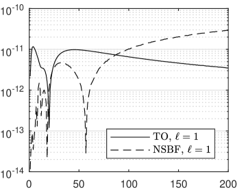
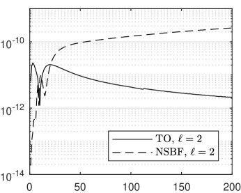
$l=5$, $N=16$		$l=10$, $N=19$

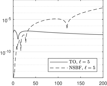
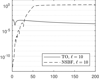
Figure 1: Absolute errors of the first 200 eigenvalues for the spectral problem (6.1), (6.2) for different values of $l$ obtained using the proposed method (solid lines, marked as TO on the legends) and those produced by the method from [10] (dashed lines, marked as NSBF on the legends). The parameter $N$ over each figure corresponds to the truncation parameter used for the approximate solution (4.6).

The obtained results confirm Remark 3, the proposed method outperforms the method from [10] for large index eigenvalues. Uniform (and even decaying) absolute error of approximate eigenvalues can be appreciated. The loss of accuracy for large values of $l$ can be easily explained from the representation (4.2). Recall that due to recurrent formulas used for computation of the coefficients $\beta_{m}$ (see [10, (6.11)]) the absolute errors of the computed coefficients $\beta_{m}$ are slowly growing as $m\to\infty$. The coefficients $\Gamma(m+2l+5/2)/\Gamma(m+l+3/2)$ also grow as $m\to\infty$. For $l=5$ the first coefficient is about $4.8\cdot 10^{5}$, while for $l=10$ the first coefficient is about $2\cdot 10^{13}$, which explains the loss of accuracy.

6.2 Non-integer $l$: approximate integral kernel

We illustrate the representation (5.1) constructing numerically the integral kernel $K$. Unfortunately we are not aware of any single nontrivial potential $q$ for which the integral kernel $K$ is known in a closed form. In [9] an analytic approximation was proposed and revealed excellent numerical performance for the potential $q(x)=x^{2}$, $x\in[0,\pi]$ and for $l=-0.5$ or $l=0.5$ (the Goursat data (1.4) was satisfied with an error less than $10^{-12}$ and a large set of eigenvalues was calculated with absolute errors smaller than $10^{-11}$). It is worth to mention that for other values of $l$, say $1/3$ or $3/2$, and for other potentials, the performance of the method from [9] was considerably worse. We consider the same potential and the same values of $l$ to illustrate the numerical behavior of the representation (5.1), using the approximate kernel $K$ obtained with the method from [9] in the role of an exact one for all the comparisons.

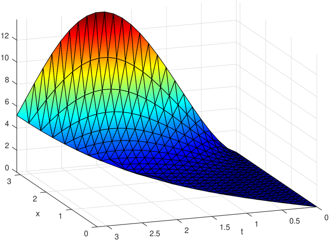
Figure 2: The integral kernel $K$ of the transmutation operator for equation (6.1) with $l=0.5$.

It is known [10, Proposition 4.5] that for non-integer values of $l$ the coefficients $\beta_{k}$ decay as $k^{-2l-3}$ when $k\to\infty$, hence the series in (5.1) converges rather slow. For that reason we computed the coefficients $\beta_{k}$ for $k\leq 150$. The necessary values of the Jacobi polynomials $P_{k}^{l+1/2,-l-1}$ were calculated using the recurrent formula (4.5.1) from [15]. It is worth to mention that the whole computation took few seconds. On Figure 2 we present the kernel $K$ for $l=0.5$. On Figure 3 we show the absolute error, the value of the difference $|K(\pi,t)-K_{150}(\pi,t)|$, $t\in[0,\pi)$ for $l=-0.5$ and $l=0.5$. The growth of the error as $t\to x$ can be explained by the division over $(x^{2}-t^{2})^{l+1}$ in (5.1). Nevertheless, a remarkable accuracy can be appreciated. The obtained approximation may be used, in particular, for solution of spectral problems, we leave the detailed analysis for a separate study.

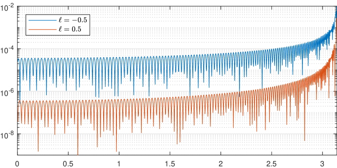
Figure 3: Absolute error of the approximate integrate kernel for equation (6.1) at $x=\pi$ obtained from the truncated representation (5.1) taking coefficients up to $k=150$, i.e., the value $|K(\pi,t)-K_{150}(\pi,t)|$, $t\in[0,\pi)$. Upper (blue) line corresponds to $l=-0.5$, lower (red) line corresponds to $l=0.5$.

References

- [1] V. Y. Volk, “On inversion formulas for a differential equation with a singularity at (in Russian),” Uspehi Matem. Nauk (N.S.) 8 (4), 141–151 (1953).
- [2] K. Chadan and P. C. Sabatier, Inverse Problems in Quantum Scattering Theory (Springer-Verlag, New York, 1989).
- [3] H. Chebli, A. Fitouhi, and M. M. Hamza, “Expansion in series of Bessel functions and transmutations for perturbed Bessel operators,” J. Math. Anal. Appl. 181 (3), 789–802 (1994).
- [4] M. Coz and Ch. Coudray, “The Riemann solution and the inverse quantum mechanical problem,” J. Math. Phys. 17 (6), 888–893 (1976).
- [5] A. Kostenko, G. Teschl and J. H. Toloza, “Dispersion Estimates for Spherical Schrödinger Equations”, Ann. Inst. Henri Poincaré 17 (11), 3147–3176, (2016).
- [6] V. V. Stashevskaya, “On the inverse problem of spectral analysis for a differential operator with a singularity at zero (in Russian),” Zap. Mat. Otdel. Fiz.-Mat.Fak.KhGU i KhMO 25 (4) 49–86 (1957).
- [7] S. M. Sitnik, “Transmutations and applications: a survey,” arXiv:1012.3741.
- [8] K. Trimeche, Transmutation operators and mean-periodic functions associated with differential operators, (Harwood Academic Publishers, 1988).
- [9] V. V. Kravchenko, S. M. Torba and J. Y. Santana-Bejarano, “Generalized wave polynomials and transmutations related to perturbed Bessel equations,” arXiv:1606:07850.
- [10] V. V. Kravchenko, S. M. Torba and R. Castillo-Pérez, “A Neumann series of Bessel functions representation for solutions of perturbed Bessel equations,” Applicable Analysis (to appear), doi:10.1080/00036811.2017.1284313.
- [11] B. M. Levitan, “Expansion in Fourier Series and Integrals with Bessel Functions (in Russian),” Uspekhi Mat. Nauk 6 (2), 102–143 (1951).
- [12] S. G. Samko, A. A. Kilbas and O. I. Marichev, Fractional Integrals and Derivatives: Theory and Applications (Gordon and Breach, Yverdon, Switzerland, 1993).
- [13] I. S. Gradstein and I. M. Ryzhik, Tables of Integrals, Sums, Series and Products, 4th ed. (in Russian) (Moscow, Fizmatgiz, 1963).
- [14] M. Abramowitz and I. A. Stegun, Handbook of Mathematical Functions with Formulas, Graphs, and Mathematical Tables, 9th printing (Dover Publications, New York, 1983).
- [15] G. Szegö, Orthogonal Polynomials, revised edition, (American Mathematical Society, New York, 1959).
- [16] H. Bateman and A. Erdelyi, Table of Integral Transforms, Vol. 2 (McGraw-Hill Book Company, New York, 1953).
- [17] A. P. Prudnikov, Y. A. Brychkov and O. I. Marichev, Integrals and Series, Vol. 2, Special Functions, 2nd ed. (in Russian) (Fizmatlit, Moskow, 2003).
- [18] R. Castillo-Pérez, V. V. Kravchenko and S. M. Torba, “Spectral parameter power series for perturbed Bessel equations,” Appl. Math. Comput. 220, 676–694 (2013).