On the Calculus of Functions with the Cantor-Tartan Support

Abstract

In this manuscript, integral and derivative of the functions with Cantor-Tartan spaces is defined. The generalization of standard calculus which is called $F^{\alpha}$-calculus utilized to obtain the integral and derivative of the functions on the Cantor-Tartan with different dimensions. Differential equation involving the new derivatives are solved. The illustrative examples are used to present the details. Keywords: $F^{\alpha}$-calculus; Staircase function ; Cantor-Tartan support; Fractional differential equation

MSC[2010]: 81Q35; 28A80;

The fractal shapes and objects are seen in the nature, e.g., clouds, mountains, coastlines, human body, and etc. The geometry of the fractals were studied [26]. The analysis on fractals were established, using different methods, such as fractional calculus, probability theory, measure theory, fractional spaces, and time scale theory by many researchers and found many applications [12, 25, 25, 6, 2, 7, 1, 31, 35, 36, 8]. The fractional derivatives have non-local property which are suitable to model the process with the memory effect, non-conservative systems [22, 23, 30, 39, 41, 24, 27, 28, 33, 18]. The fractional calculus, which involves derivatives with arbitrary orders, has applied on the process with fractals structures [37, 29, 9]. The anomalous diffusion on fractals was formulated which included sub- and supper diffusion in view of different random walks [40, 11, 38]. Fractal antennas are small but have wide-band radiations which make them useful in microwave communications [21, 10]. Laminar flow of a fractal fluid in a cylindrical tube was studied using the homogeneous flow in a fractional dimensional space [4]. On the Cantor cubes, the Maxwell’s equation were obtained and, as an application, the electric field due to Cantor dust was obtained [5]. Recently, $F^{\alpha}$-calculus which is algorithmic was suggest and applied for modeling some physical process [32, 34]. As a pursuit of these researches, $F^{\alpha}$-calculus is generalized and utilized in optics and mechanics [13, 14, 15, 3]. The non-local integrals and derivatives are defined on the Cantor set which are used to model the fractal ideal solids and the fractal ideal fluids [16, 17].
This manuscript is built as follows:
In Section 1 we set up the notation and terminology of $F^{\alpha}$-calculus on the fractals that imbedded in $\Re^{2}$ [19, 20]. In Section 2 we study some examples on the Cantor-Tartan using suggested definitions. Section 3 is devoted to the conclusion.

1 Terminology and notations

In the section, we review and define the basic tools we need in our work.
Fractals are the sets with the self-similar properties such that theirs fractal dimension exceeds from theirs topological dimension. The calculus on the Cantor-Tartan $\mathfrak{F}=F\cup F\subset\Re^{2}$ where $F=C\times\Re$, $C$ is Cantor set and $\Re$ is real line [12]. Let $\mathfrak{F}$ be Cantor-Tartan that is subset of $I=[a,b]\times[c,d],~{}a,~{}b,~{}c,~{}d\in\Re$ (Real-line). We sketch in Figures [1] the Cantor-Tartan with different fractal box or similar dimensions. The Cantor-Tartan is established by Cartesian product of Cantor set and real line (F) and union of them. Here, we consider finite iteration which is approximation of fractals spaces.

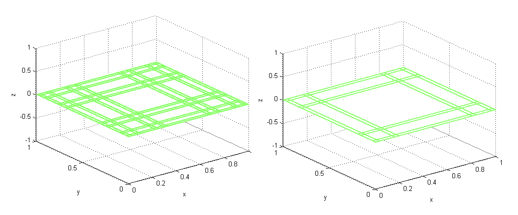
Figure 1: The Cantor-Tartan with different dimensions are plotted.

The flag function for the Cantor-Tartan $\mathfrak{F}=F\cup F\subset\Re^{2}$, which is denoted by $\Theta(\mathfrak{F},I)$, is defined as follows

$$\Theta(\mathfrak{F},I)=\begin{cases}1,~{}~{}~{}\textmd{if}~{}~{}~{}\mathfrak{F}\cap I\neq\emptyset,\\ 0,~{}~{}~{}~{}\textmd{otherwise}.\end{cases}$$ (1)

The subdivision $P_{[a,b]}$ is

$$P_{[a,b]\times[c,d]}=\{x_{0}=a,x_{1},x_{2},...,x_{n}=b\}\times\{y_{0}=c,y_{1},y_{2},...,~{}y_{m}=d\},$$ (2)

where $\times$ denotes the Cartesian product.
The $\gamma^{\zeta}(\mathfrak{F},a,b,c,d)$ is defined

$$\gamma^{\zeta}(\mathfrak{F},a,b,c,d)=$$

$$\lim_{\delta\rightarrow 0}\inf_{P_{[a,b]\times[c,d]}:|P|\leq\delta}\sum_{j=1}^{n}\sum_{i=1}^{n}\frac{(x_{i}-x_{i-1})^{\alpha}}{\Gamma(\alpha+1)}\frac{(y_{j}-y_{j-1})^{\beta}}{\Gamma(\beta+1)}~{}\Theta(\mathfrak{F},[x_{i-1},x_{i}])~{}\Theta(\mathfrak{F},[y_{j-1},y_{j}]),$$ (3)

where $\zeta=\max\{\alpha+\beta\}$, $\alpha=\beta=1+Dim(C)$ and $|P|$ is

$$|P|=\max_{1\leq i\leq n,~{}1\leq j\leq n}(x_{i}-x_{i-1})\times(x_{j}-x_{j-1}).$$ (4)

The integral staircase function $S_{\mathfrak{F}}^{\zeta}(x,y)$ for Cantor-Tartan $\mathfrak{F}$ is defined

$$S_{F}^{\zeta}(x,y)=\begin{cases}\gamma^{\zeta}(F,a_{0},c_{0},x,y),~{}~{}~{}~{}\text{if},~{}~{}~{}~{}~{}x\geq a_{0},~{}~{}y\geq c_{0};\\ -\gamma^{\zeta}(F,a_{0},c_{0},x,y),~{}~{}~{}~{}\text{otherwise},\end{cases}$$ (5)

where $a_{0},~{}c_{0}$ are arbitrary real numbers.

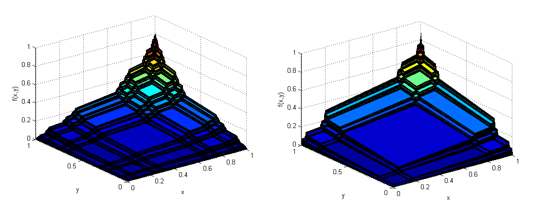
Figure 2: Staircase function corresponding to Cantor-Tartan with different dimensions are presented.

The integral staircase function for the different Cantor-Tartan with the different dimension are plotted in Figure [2].
The $\zeta$-dimension of $\mathfrak{F}\cap[a,b]\times[c,d]$ is given by

$$\dim_{\zeta}(\mathfrak{F}\cap[a,b]\times[c,d]) = \inf\{\zeta:\gamma^{\zeta}(\mathfrak{F},a,c,b,d)=0\},$$

$$= \sup\{\zeta:\gamma^{\zeta}(\mathfrak{F},a,c,b,d)=\infty\}.$$

A point $(x,y)$ is called a point of change of a function $f(x,y)$ if it is not constant over any open set $[a,b]\times[c,d]$ involving $(x,y)$. The set of all points of change of $f(x,y)$ are indicated by $Schf$.
The $Sch(S_{\mathfrak{F}}^{\zeta}(x,y))$ is called $\zeta$-perfect if $S_{\mathfrak{F}}^{\zeta}(x,y)$ is finite for all $(x,y)\in\Re$.
Let $f(x,y)$ be a bounded function on $\mathfrak{F}$ then we define

$$M[f,\mathfrak{F},I] = \sup_{(x,y)\in\mathfrak{F}\cap I}f(x,y),~{}~{}~{}~{}\text{if}~{}~{}~{}\mathfrak{F}\cap I\neq 0.$$

$$= 0,~{}~{}~{}~{}~{}\text{otherwise},$$

and similarly

$$m[f,\mathfrak{F},I] = \inf_{(x,y)\in\mathfrak{F}\cap I}f(x,y),~{}~{}~{}~{}\text{if}~{}~{}~{}\mathfrak{F}\cap I\neq 0.$$

$$= 0,~{}~{}~{}~{}~{}\text{otherwise}.$$

Now, upper $U^{\zeta}$-sum and lower $L^{\zeta}$-sum for the function $f(x,y)$ over the subdivision $P$ are given as follows

$$U^{\zeta}[f,\mathfrak{F},P]=\sum_{i=1}^{n}M[f,\mathfrak{F},[(x_{i-1},y_{i-1}),(x_{i},y_{i})]](S_{\mathfrak{F}}^{\zeta}(x_{i},y_{i})-S_{\mathfrak{F}}^{\zeta}(x_{i-1},y_{i-1})),$$ (9)

and

$$L^{\zeta}[f,\mathfrak{F},P]=\sum_{i=1}^{n}m[f,\mathfrak{F},[(x_{i-1},y_{i-1}),(x_{i},y_{i})]](S_{\mathfrak{F}}^{\zeta}(x_{i},y_{i})-S_{\mathfrak{F}}^{\zeta}(x_{i-1},y_{i-1})).$$ (10)

The $f(x,y)$ is called $F^{\zeta}$-integrable on Cantor-Tartan $\mathfrak{F}$ if we have

$$\underline{\int_{(a,c)}^{(b,d)}}f(x,y)d_{F}^{\alpha}xd_{F}^{\beta}y=\sup_{P_{[a,b]}}L^{\zeta}[f,\mathfrak{F},P]=\overline{\int_{(a,c)}^{(b,)d}}f(x,y)d_{F}^{\alpha}xd_{F}^{\beta}y=\inf_{P_{[a,b]}}L^{\zeta}[f,\mathfrak{F},P].$$ (11)

The $F^{\zeta}$-integral is denoted by $\int_{(a,b)}^{(b,d}f(x,y)d_{F}^{\alpha}xd_{F}^{\beta}y$.
Let $\mathfrak{F}$ be $\zeta$-perfect set then we define $F^{\alpha}$-partial derivative of $f(x,y)$ respect to $x$ as

$${}^{x}D_{\mathfrak{F}}^{\alpha}f(x,y)=\begin{cases}\mathfrak{F}-\lim_{(x^{\prime},y)\rightarrow(x,y)}\frac{f(x^{\prime},y)-f(x,y)}{S_{\mathfrak{F}}^{\zeta}(x^{\prime},y)-S_{\mathfrak{F}}^{\zeta}(x,y)},~{}~{}~{}\text{if}~{}~{}~{}(x,y)\in\mathfrak{F},\\ 0,~{}~{}~{}~{}~{}~{}~{}~{}~{}~{}~{}~{}~{}\textmd{otherwise}.\end{cases}$$ (12)

if the limit exists.

2 The functions with Cantor-Tartan support

The task is now to apply definitions on examples. In this section, we give some examples to show more details.

2.1 Example 1.

Let us consider a function with Cantor-Tartan support with the different fractal dimensions

$$f(x,y)=\sin(\chi_{F}^{\alpha}x)\sin(\chi_{F}^{\beta}y),~{}(x,y)\in\mathfrak{F},$$ (13)

where $\chi_{F}^{\alpha},~{}\chi_{F}^{\beta}$ are characteristic function for fractal sets $F$ [17, 32]. The graph of the $f(x,y)$ is shown in Figures [3].

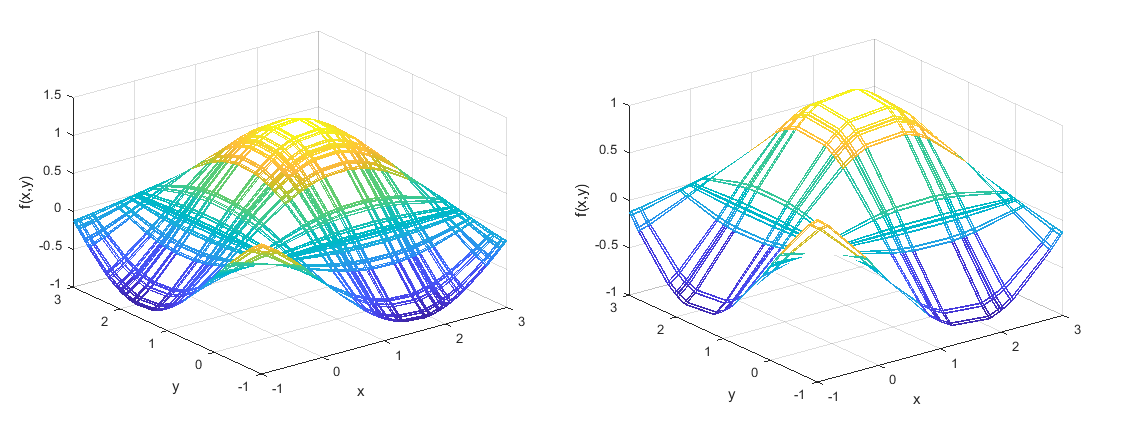
Figure 3: We plot the graph of function $\sin(\chi_{F}^{\alpha}x)\sin(\chi_{F}^{\beta}y)$ with the different Cantor-Tartan support.

The fractal integral of $f(x,y)$ on Cantor-Tartan $\mathfrak{F}\subset[0,1]\times[0,1]$ is as follows:

$$g(x,y)\bigg{|}_{(x=y=1)}=\int_{0}^{x}\int_{0}^{y}\sin(\chi_{F}^{\alpha}x)\sin(\chi_{F}^{\beta}y)d_{F}^{\alpha}x^{\prime}d_{F}^{\beta}y^{\prime}\bigg{|}_{(x=y=1)}=$$

$$\int_{0}^{1}\cos(S_{F}^{\beta}(y^{\prime}))\sin(\chi_{F}^{\alpha}x)\bigg{|}_{0}^{1}d_{F}^{\alpha}x^{\prime}=$$

$$\int_{0}^{1}[\cos(S_{F}^{\beta}(1))\sin(\chi_{F}^{\alpha}x)-\cos(S_{F}^{\beta}(0))\sin(\chi_{F}^{\alpha}x)]~{}d_{F}^{\alpha}x^{\prime}=$$

$$\cos(\Gamma(1+\beta))\cos(S_{F}^{\alpha}(x^{\prime}))-\cos(S_{F}^{\alpha}(x^{\prime}))\bigg{|}_{S_{F}^{\alpha}(0)}^{S_{F}^{\alpha}(1)}=$$

$$\cos(\Gamma(1+\beta))\cos(\Gamma(1+\alpha))-\cos(\Gamma(1+\alpha))-\cos(\Gamma(1+\beta))+1$$

$$=\left\{\begin{array}[]{ll}0.13,&\alpha=\beta=0.6~{}~{}\textmd{With~{}support~{}Cantor-Tartan~{}dimesion~{} 1.2}\\ 0.16,&\alpha=\beta=0.8~{}~{}\textmd{With~{}support~{}Cantor-Tartan dimesion ~{}1.6}\end{array}\right.$$ (16)

here $S_{F}^{\alpha}(1)=\Gamma(1+\alpha),~{}S_{F}^{\beta}(1)=\Gamma(1+\beta),~{}S_{F}^{\alpha}(0)=S_{F}^{\beta}(0)=0$ .

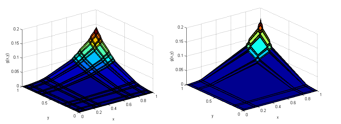
Figure 4: Fractal integral of $\sin(\chi_{F}^{\alpha}x)\sin(\chi_{F}^{\beta}y)$ on the different Cantor-Tartan are sketched .

In Figure [4] we sketch the $g(x,y)$ which is called fractal integral of $f(x,y)$.

2.2 Example 2.

Consider a function with Cantor-Tartan support as follows

$$f(x,y)=\sin(\chi_{F}^{\alpha}x+\chi_{F}^{\beta}y),~{}(x,y)\in\mathfrak{F}$$ (17)

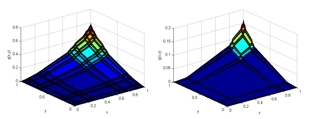
Figure 5: We plot the graph of function $\sin(\chi_{F}^{\alpha}x+\chi_{F}^{\beta}y)$ with the different Cantor-Tartan support.

We present in Figure [5] graph of Eq. (17). The fractal integral of Eq. (17) is as follows

$$g(x,y)\bigg{|}_{(x=y=1)}=\int_{0}^{x}\int_{0}^{y}\sin(\chi_{F}^{\alpha}x+\chi_{F}^{\beta}y)d_{F}^{\alpha}x^{\prime}~{}d_{F}^{\beta}y^{\prime}\bigg{|}_{(x=y=1)}=$$

$$\int_{0}^{1}-\cos(\chi_{F}^{\alpha}x+S_{F}^{\beta}(y))\bigg{|}_{0}^{1}d_{F}^{\alpha}x^{\prime}=$$

$$\int_{0}^{1}[-\cos(\chi_{F}^{\alpha}x+S_{F}^{\beta}(1))+\cos(\chi_{F}^{\alpha}x)]~{}d_{F}^{\alpha}x^{\prime}=$$

$$-\sin(S_{F}^{\alpha}(x^{\prime})+\Gamma(1+\beta))+\sin(S_{F}^{\alpha}(x^{\prime}))\bigg{|}_{0}^{1}=$$

$$=-\sin(\Gamma(1+\alpha)+\Gamma(1+\beta))+\sin(\Gamma(1+\alpha))+\sin(\Gamma(1+\beta))$$

$$=\left\{\begin{array}[]{ll}0.581,&\alpha=\beta=0.6~{}~{}\textmd{With~{}support~{}Cantor-Tartan~{}dimesion~{} 1.2}\\ 0.64,&\alpha=\beta=0.8~{}~{}\textmd{With~{}support~{}Cantor-Tartan dimesion ~{}1.6}\end{array}\right.$$ (20)

where $S_{F}^{\alpha}(1)=\Gamma(1+\alpha),~{}S_{F}^{\beta}(1)=\Gamma(1+\beta),~{}S_{F}^{\alpha}(0)=S_{F}^{\beta}(0)=0$.

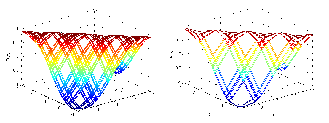
Figure 6: Fractal integral of $\sin(\chi_{F}^{\alpha}x+\chi_{F}^{\beta}y)$ on different Cantor-Tartan are shown.

In Figure [6] we plot fractal integral of $\sin(\chi_{F}^{\alpha}x+\chi_{F}^{\beta}y)$ versus to different Cantor-Tartan support with different dimensions.

2.3 Example 3.

Consider a function with the Cantor-Tartan as follows

$$f(x,y)=S_{F}^{\alpha}(x)^{2}+S_{F}^{\beta}(y)^{2}.$$ (21)

The fractal partial derivatives of $f(x,y)$ respect to $x$ and $y$ are

$$^{x}D^{\alpha}_{F}f(x,y)=2S_{F}^{\alpha}(x)\chi_{F},~{}~{}~{}^{y}D^{\alpha}_{F}f(x,y)=2S_{F}^{\alpha}(y)\chi_{F}.$$ (22)

In Figure [7] we plot Eq. (21) and it’s partial derivative which is shown ${}^{x}D^{\alpha}_{F}(x,y)$.

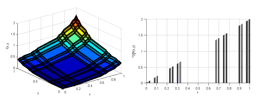
Figure 7: We have plotted $S_{F}^{\alpha}(x)^{2}+S_{F}^{\beta}(y)^{2}$ and ${}^{x}D^{\alpha}_{F}(x,y)$.

Remark: One can obtain standard results by choosing $\alpha=1,~{}\beta=1,~{}S=\Re$ which leads to $S_{F}^{\alpha}(x)=x,~{}S_{F}^{\beta}(y)=y$.

3 Conclusion

In this work, we define the local derivative and integral on Cantor-Tartan. The standard calculus can not be applied to integrate and differentiate for the function on this fractals. Therefore, we need a new type of calculus to calculate the physical properties and describe phenomena on fractals. As a result, the $F^{\alpha}$-calculus on Cantor-Tartan which has fractal dimension $1<\zeta<2$ is given. More, we recall the standard calculus results which shows that suggested definitions are the generalization of standard calculus. Three illustrative examples were investigated and the corresponding graphs of the functions were drawn.

References

- [1] Agarwal RP, Bohner M. Basic calculus on time scales and some of its applications. Results Math 1999; 35: 3-22.
- [2] Agarwal RP, Mahmoud RR, Saker SH, Tunc C. Acta Math Hung 2017; 152: 383-403.
- [3] Ashrafi S, Golmankhaneh A. K. Energy straggling function by -calculus. ASME, J Comput Nonlinear Dynam 2017, doi:10.1115/1.4035718.
- [4] Balankin AS, Mena B, Susarrey O, Samayoa D. Steady laminar flow of fractal fluids. Phys Lett A 2017; 381: 623-628.
- [5] Balankin AS, Mena B, Patino J, Morales D. Electromagnetic fields in fractal continua. Phys Lett A 2013; 377: 783-788.
- [6] Bohner M, Peterson A, Dynamic Equations on Time Scales: An Introduction with Applications. Birkhäuser, Boston 2001.
- [7] Bohner M, Wintz N. The linear quadratic tracker on time scales. Int J Dyn Syst Differ Equ 2011; 3: 423-447.
- [8] Brossard J, Carmona R. Can one hear the dimension of fractal?. Comm Math Phys 1986; 104: 103-122.
- [9] Butera S, Paola MD. A physically based connection between fractional calculus and fractal geometry. Ann Phys-New York 2014; 350: 146-158.
- [10] Cohen N. Fractal antenna applications in wireless telecommunications. Electronics Industries Forum of New England, IEEE, 1997.
- [11] Chen W, Sun HG, Zhang X, Koroak D. Anomalous diffusion modeling by fractal and fractional derivatives. Comp Math Appl 2010; 59: 1754-1758.
- [12] Falconer K. Techniques in Fractal Geometry. John Wiley and Sons, 1997.
- [13] Golmankhaneh AK, Baleanu D. Diffraction from fractal grating Cantor sets. J Mod Optic 2016; 63:1364-1369.
- [14] Golmankhaneh AK, Baleanu D. Fractal calculus involving Gauge function. Commun Nonlinear Sci 2016; 37: 125-130.
- [15] Golmankhaneh A K, Tunc C. On the Lipschitz condition in the fractal calculus. Chaos Soliton Fract. 2017; 95: 140-147.
- [16] Golmankhaneh AK, Baleanu D. New derivatives on the fractal subset of Real-line. Entropy, 2016; 18: 1-13.
- [17] Golmankhaneh AK,Baleanu D. Non-local Integrals and Derivatives on Fractal Sets with Applications. Open Phys 2016; 14: 542-548.
- [18] Golmankhaneh A K. Investigations in Dynamics: With Focus on Fractional Dynamics. LAP Lambert Academic Publishing, Saarbrucken, 2012.
- [19] Golmankhaneh AK. About Kepler’s Third Law on fractal-time spaces. Ain Shams Eng J doi:/10.1016/j.asej.2017.06.005
- [20] Golmankhaneh A K. On the calculus of the parameterized fractal curves. Turk J Phys 2017; 41: 418-425.
- [21] Gianvittorio JP, Rahmat-Samii Y. Fractal antennas: A novel antenna miniaturization technique and applications. IEEE Antennas Propag 2002; 44: 20-36.
- [22] Herrmann R. Fractional calculus: an introduction for physicists. World Scientific, 2014.
- [23] Hilfer R ed. Applications of fractional calculus in physics. World Scientific, 2000.
- [24] Kilbas AA, Srivastava HH, Trujillo JJ. Theory and Applications of Fractional Differential Equations. Elsevier, The Netherlands, 2006.
- [25] Kigami J. Analysis on fractals. Volume 143 of Cambridge Tracts in Mathematics, Cambridge University Press, Cambridge, 2001.
- [26] Mandelbrot BB. The Fractal Geometry of Nature. Freeman and Company, 1977.
- [27] Magin RL. Fractional Calculus in Bioengineering. Begell House Publisher, Inc. Connecticut, 2006.
- [28] Malinowska AB, Torres DFM. Introduction to the fractional calculus of variations. Imperial College Press, London, 2012.
- [29] Nigmatullin RR, Zhang W, Gubaidullin I. Accurate relationships between fractals and fractional integrals: new approaches and evaluations. Fract Calculus Appl Anal 2017; 20: 1263-1280.
- [30] Nigmatullin RR, Evdokimov YK. The concept of fractal experiments: New possibilities in quantitative description of quasi-reproducible measurements. Chaos Soliton Fract 2016; 91: 319-328.
- [31] Naqvi QA, Fiaz MA. Electromagnetic behavior of a planar interface of non-integer dimensional spaces. J Electromag Waves Appl 2017; 31: 625-1637.
- [32] Parvate A, Gangal A D. Calculus on fractal subsets of real line II: Conjugacy with ordinary calculus. Fractals 2011; 19: 271-290.
- [33] Podlubny I. Fractional differential equations. Academic Press, New York, 1999.
- [34] Seema S, Gangal AD. Langevin Equation on Fractal Curves, Fractals. 2016; 24: 1650028.
- [35] Strichartz RS. Differential equations on fractals: a tutorial, Princeton University Press, 2006.
- [36] Tarasov VE, Fractional dynamics: applications of fractional calculus to dynamics of particles, fields and media, Springer Science, 2011.
- [37] Tatom FB. The relationship between fractional calculus and fractals. Fractals 1995; 3: 217-229.
- [38] Telcs A. The art of random walks. Springer, New York, 2006.
- [39] Uchaikin VV. Fractional Derivatives for Physicists and Engineers Vol. 1 Background and Theory. Vol 2. Application Springer, Berlin, 2013.
- [40] Von Kameke A, Huhn F, Fernández-García G, Muñuzuri, V. Pérez-Muñuzuri AP. Propagation of a chemical wave front in a quasi-two-dimensional superdiffusive flow. Phys Rev E 2010; 81: 066211.
- [41] Wu GC, Baleanu D, Xie HP, Chen FL. Chaos synchronization of fractional chaotic maps based on stability results. Physica A 2016; 460: 374-383.