Error analysis of a fully discrete Morley finite element approximation for the Cahn-Hilliard equation

Abstract

This paper proposes and analyzes the Morley element method for the Cahn-Hilliard equation. It is a fourth order nonlinear singular perturbation equation arises from the binary alloy problem in materials science, and its limit is proved to approach the Hele-Shaw flow. If the $L^{2}(\Omega)$ error estimate is considered directly as in paper elliott1989nonconforming , we can only prove that the error bound depends on the exponential function of $\frac{1}{\epsilon}$. Instead, this paper derives the error bound which depends on the polynomial function of $\frac{1}{\epsilon}$ by considering the discrete $H^{-1}$ error estimate first. There are two main difficulties in proving this polynomial dependence of the discrete $H^{-1}$ error estimate. Firstly, it is difficult to prove discrete energy law and discrete stability results due to the complex structure of the bilinear form of the Morley element discretization. This paper overcomes this difficulty by defining four types of discrete inverse Laplace operators and exploring the relations between these discrete inverse Laplace operators and continuous inverse Laplace operator. Each of these operators plays important roles, and their relations are crucial in proving the discrete energy law, discrete stability results and error estimates. Secondly, it is difficult to prove the discrete spectrum estimate in the Morley element space because the Morley element space intersects with the $C^{1}$ conforming finite element space but they are not contained in each other. Instead of proving this discrete spectrum estimate in the Morley element space, this paper proves a generalized coercivity result by exploring properties of the enriching operators and using the discrete spectrum estimate in its $C^{1}$ conforming relative finite element space, which can be obtained by using the spectrum estimate of the Cahn-Hilliard operator. The error estimate in this paper provides an approach to prove the convergence of the numerical interfaces of the Morley element method to the interface of the Hele-Shaw flow.

1 Introduction

Consider the following Cahn-Hilliard problem:

$$u_{t}+\Delta(\epsilon\Delta u-\frac{1}{\epsilon}f(u)) =0 \quad\mbox{in }\Omega_{T}:=\Omega\times(0,T],$$ (1)

$$\frac{\partial u}{\partial n}=\frac{\partial}{\partial n}(\epsilon\Delta u-\frac{1}{\epsilon}f(u)) =0 \quad\mbox{on }\partial\Omega_{T}:=\partial\Omega\times(0,T],$$ (2)

$$u =u_{0} \quad\mbox{in }\Omega\times\{t=0\},$$ (3)

where $\Omega\subseteq\mathbf{R}^{2}$ is a bounded domain, $f(u)$ is the first derivative of a double well potential $F(u)$ which is defined below

$$F(u)=\frac{1}{4}(u^{2}-1)^{2}.$$ (4)

The Allen-Cahn equation Allen_Cahn79 ; Bartels_Muller_Ortner09 ; Chen94 ; Feng_Prohl03 ; feng2014finite ; feng2017finite ; Ilmanen93 ; kovacs2011finite , which is a second order nonlinear parabolic equation, describes the phase separation process of a binary alloy when the temperature suddenly decreases, but the mass of each phase is not conserved. Compared with the Allen-Cahn equation, the Cahn-Hilliard equation (1) also arises from the phase transition problem in materials science, but it has the mass conservation property. Notice equation (1) differs from the original Cahn-Hilliard equation by scaling $\frac{t}{\epsilon}$ by $t$. The Cahn-Hilliard equation finds its applications in the areas of materials science, fluid mechanics, biology and so on, and the coupling of the Cahn-Hilliard equation and fluid flow is becoming more and more popular in industrial applications. The Cahn-Hilliard equation also serves as a building block for the phase field formulations of the moving interface problems, and the methodology can be applied to other phase field models. It is also well known Alikakos94 that the Cahn-Hilliard equation (1) can be interpreted as the $H^{-1}$ gradient flow of the Cahn-Hilliard energy functional

$$J_{\epsilon}(v):=\int_{\Omega}\Bigl{(}\frac{\epsilon}{2}|\nabla v|^{2}+\frac{1}{\epsilon}F(v)\Bigr{)}\,dx.$$ (5)

Stoth proved that $u\rightarrow\pm 1$ in the interior or exterior of interface $\Gamma_{t}$ for all $t\in[0,T]$ as $\epsilon\rightarrow 0$ for the radially symmetric case Stoth96 , and Alikakos, Bates and Chen gave the proof for the general case Alikakos94 .

Numerical approximations of the Cahn-Hilliard equation have been extensively studied during the last 30 years Aristotelous12 ; xu2016convex ; du1991numerical ; elliott1989nonconforming ; cheng2017energy . These papers consider the case when $\epsilon$ is a fixed, and the error bounds depend exponentially on $\frac{1}{\epsilon}$. Better than the exponential dependence on $\frac{1}{\epsilon}$, the polynomial dependence on $\frac{1}{\epsilon}$ is proved using conforming finite element (CG) method Feng_Prohl04 ; Feng_Prohl05 and discontinuous Galerkin (DG) method feng2016analysis ; li2015numerical . For the $C^{1}$ conforming finite elements for the fourth order problem, polynomials with high degree are required. To use lower order polynomials, one approach is to use macro-elements, where a given element is divided into a few smaller subelements and the lower order polynomial is used on each subelement. However, it is not widely used due to its complex formulation of finite element spaces. The other approach is to use nonconforming finite elements, and among the nonconforming finite elements, the Morley element has the least number of degrees of freedom on each element. Comparing with the mixed finite element method or the $C^{1}$ conforming finite element method, the computational cost of the Morley element is smaller, and this is extremely important especially for the phase field problems where the interaction length $\epsilon$, time step size $k$, and mesh size $h$ are all required to be chosen very small. The Morley element was first used in elliott1989nonconforming to discretize the Cahn-Hilliard equation, but only the error estimates with exponential dependence of $\frac{1}{\epsilon}$ could be derived there. In this paper, the polynomial dependence of $\frac{1}{\epsilon}$ is finally given using the Morley element.

The approach in this paper follows those used in feng2016analysis ; Feng_Prohl04 ; Feng_Prohl05 , but the generalization to the Morley element method is nontrivial. In the mixed CG/DG formulation, different test functions can be chosen in two equations, but in the Morley element formulation, only one test function can be chosen. Because of this and the complex structure of the Morley element formulation, proving the discrete energy law and the discrete stability results become much more involved. It is also a challenge to prove the discrete spectrum estimate in the Morley element space from the spectrum estimate of the Cahn-Hilliard operator because the Morley element space has intersection with its $C^{1}$ conforming relative finite element space but they are not contained in each other. If the $L^{2}$ error estimate is considered directly, the generalized coercivity result in this paper or even the discrete spectrum estimate are not useful in proving the $L^{2}$ error estimate. To overcome these difficulties, there are three main techniques in this paper. First, based on the structure of the bilinear form of the Morley element formulation, this paper designs four discrete operators $\hat{\Delta}^{-1}_{h},\widetilde{\Delta}^{-1}_{h}$, $\underline{\Delta}^{-1}_{h}$ and $\Delta^{-1}_{h}$, and proves the errors in different norms between these operators. Through these relations, by using $\widetilde{\Delta}^{-1}_{h}$ in the test function, and by using the other operators as bridges, we can prove the discrete energy law and some consequent discrete stability results. Each of these operators plays important roles in proving the main results. These operators and their properties might be applied to the analysis for the biharmonic equation. It also employs both the summation by part for time and integration by part for space techniques to handle the nonlinear term and then to establish the polynomial dependence of the $\|\cdot\|_{2,2,h}$ stability result, and only the exponential dependence can be obtained if these two techniques are not used simultaneously. Second, instead of proving the discrete spectrum estimate, this paper proves the generalized coercivity result which is sufficient to get the sharper error estimates. The key point is to use the enriching operator as a bridge between the nonconforming and conforming finite elements, and this idea may be extended to other phase field models. Third, if the discrete $L^{2}$ error estimate is considered directly, only the error estimates with exponential dependence on $\frac{1}{\epsilon}$ could be derived using the Gronwall’s inequality as in elliott1989nonconforming . This paper provides a possibility by considering the $H^{-1}$ error estimate first, and it explains how to utilize the discrete inverse Laplace operators and the generalized coercivity result to circumvent the Gronwall’s inequality, and finally to prove the error estimate with polynomial dependence on $\frac{1}{\epsilon}$.

The remainder of this paper is organized as follows. In section 2, we introduce the standard function and Sobolev space notations, state a few a priori estimates of the solution, and cite some known results including properties of the inverse Laplapce operators, properties of enriching operator, generalized discrete Gronwall’s inequality and the spectrum estimate for the linearized Cahn-Hilliard operator; In section 3, and in the first two subsections, we introduce the Morley element formulation, define different kinds of discrete inverse Laplace operators and state their relations. Then in the last three subsections, we analyze the discrete energy law and the discrete stability results, derive the generalized coercivity result in the Morley element space, and finally prove the discrete $H^{-1}$ error estimate with polynomial dependence on $\frac{1}{\epsilon}$; In Section 4, numerical experiments are given to validate the theoretical results.

2 Preliminaries

In this section, we cite some known results about problem (1)–(4), and they will be used in the following sections. These results can be proved under some general assumptions on the initial condition Chen94 ; Feng_Prohl04 ; Feng_Prohl05 ; feng2016analysis ; li2015numerical . Throughout this paper, $C$ denotes a generic positive constant, which may have different values at different occasions, is independent of interfacial length $\epsilon$, spacial size $h$, and time step size $k$. The following Sobolev notations are used in this paper, i.e., for any set $A$,

$$\|v\|_{0,p,A} =\bigg{(}\int_{A}|v|^{p}dx\bigg{)}^{1/p}\qquad 1\leq p<\infty,$$

$$\|v\|_{0,\infty,A} =\underset{A}{\mbox{\rm ess sup }}|v|,$$

$$|v|_{m,p,A} =\bigg{(}\sum_{|\alpha|=m}\|D^{\alpha}v\|_{0,p,A}^{p}\bigg{)}^{1/p}\qquad 1\leq p<\infty,$$

$$\|v\|_{m,p,A} =\bigg{(}\sum_{j=0}^{m}|v|_{m,p,A}^{p}\bigg{)}^{1/p}.$$

If $A$ is the whole domain, i.e., $A=\Omega$, then $\|\cdot\|_{H^{k}},\|\cdot\|_{L^{k}}$ are used to simplify the notations $\|\cdot\|_{H^{k}(\Omega)},\|\cdot\|_{L^{k}(\Omega)}$ respectively. Besides, assume $\mathcal{T}_{h}$ to be a family of quasi-uniform triangulations of domain $\Omega$, and $\mathcal{E}_{h}$ to be a collection of edges, then for any triangle $K\in\mathcal{T}_{h}$, define the following mesh dependent semi-norm, norm and inner product

$$|v|_{j,p,h} =\bigg{(}\sum_{K\in\mathcal{T}_{h}}|v|_{j,p,K}^{p}\bigg{)}^{1/p},$$

$$\|v\|_{j,p,h} =\bigg{(}\sum_{K\in\mathcal{T}_{h}}\|v\|_{j,p,K}^{p}\bigg{)}^{1/p},$$

$$(w,v)_{h} =\sum_{K\in\mathcal{T}_{h}}\int_{K}w(x)v(x)dx.$$

Theoretically, the $tanh$ profile of the initial condition $u_{0}$ is required to prove the relations between the Cahn-Hilliard equation and the Hele-Shaw flow Alikakos94 ; Chen94 . Because of the $tanh$ profile, the following assumptions can be made on the initial condition, and they were used to derive a priori estimates for the solution of problem (1)–(4) feng2016analysis ; Feng_Prohl04 ; Feng_Prohl05 ; li2015numerical .

General Assumption (GA)

• Assume that $m_{0}\in(-1,1)$ where

  $$m_{0}:=\frac{1}{|\Omega|}\int_{\Omega}u_{0}(x)dx.$$ (6)

• There exists a nonnegative constant $\sigma_{1}$ such that

  $$J_{\epsilon}(u_{0})\leq C\epsilon^{-2\sigma_{1}}.$$ (7)

• There exists nonnegative constants $\sigma_{2}$, $\sigma_{3}$ and $\sigma_{4}$ such that

  $$\big{\|}-\epsilon\Delta u_{0}+\epsilon^{-1}f(u_{0})\big{\|}_{H^{\ell}}\leq C\epsilon^{-\sigma_{2+\ell}}\qquad\ell=0,1,2.$$ (8)

Under the above assumptions, the following a priori estimates of the solution were proved in feng2016analysis ; Feng_Prohl04 ; Feng_Prohl05 ; li2015numerical .

Theorem 2.1

The solution $u$ of problem (1)–(4) satisfies the following energy estimate:

$$\underset{t\in[0,T]}{\mbox{\rm ess sup }}\Bigl{(}\frac{\epsilon}{2}\|\nabla u\|_{L^{2}}^{2}+\frac{1}{\epsilon}\|F(u)\|_{L^{1}}\Bigr{)}+\begin{cases}\int_{0}^{T}\|u_{t}(s)\|_{H^{-1}}^{2}\,ds\\ \int_{0}^{T}\|\nabla w(s)\|_{L^{2}}^{2}\,ds\end{cases}\leq J_{\epsilon}(u_{0}).$$ (9)

Moreover, suppose that (6)–(8) hold, $u_{0}\in H^{4}(\Omega)$ and $\partial\Omega\in C^{2,1}$, then $u$ satisfies the additional estimates:

$$\frac{1}{|\Omega|}\int_{\Omega}u(x,t)\,dx=m_{0}\quad\forall t\geq 0,$$ (10)

$$\underset{t\in[0,T]}{\mbox{\rm ess sup }}\|\nabla\Delta u\|_{L^{2}}\leq C\epsilon^{-\max\{\sigma_{1}+\frac{5}{2},\sigma_{3}+1\}}.$$ (11)

Furthermore, if there exists $\sigma_{5}>0$ such that

$$\mathop{\rm{lim}}_{s\rightarrow 0^{+}}\limits\|\nabla u_{t}(s)\|_{L^{2}}\leq C\epsilon^{-\sigma_{5}},$$ (12)

then there holds

$$\int_{0}^{T}\|u_{tt}\|_{H^{-1}}^{2}ds\leq C\tilde{\rho}_{1}(\epsilon),$$ (13)

where

$$\tilde{\rho}_{1}(\epsilon) :=\epsilon^{-\frac{1}{2}\max\{2\sigma_{1}+5,2\sigma_{3}+2\}-\max\{2\sigma_{1}+\frac{13}{2},2\sigma_{3}+\frac{7}{2},2\sigma_{2}+4\}+1}+\epsilon^{-2\sigma_{5}+1}$$

$$\qquad+\epsilon^{-\max\{2\sigma_{1}+7,2\sigma_{3}+4\}+1}.$$

The next lemma gives an $\epsilon$-independent low bound for the principal eigenvalue of the linearized Cahn-Hilliard operator, and a proof of this lemma can be found in Chen94 .

Lemma 1

Suppose that (6)–(8) hold. Given a smooth initial curve/surface $\Gamma_{0}$, let $u_{0}$ be a smooth function satisfying $\Gamma_{0}=\{x\in\Omega;u_{0}(x)=0\}$ and some profile described in Chen94 . Let $u$ be the solution to problem (1)–(4). Define $\mathcal{L}_{CH}$ as

$$\mathcal{L}_{CH}:=\Delta\left(\epsilon\Delta-\frac{1}{\epsilon}f^{\prime}(u)I\right).$$ (14)

Then there exists $0<\epsilon_{0}<<1$ and a positive constant $C_{0}$ such that the principle eigenvalue of the linearized Cahn-Hilliard operator $\mathcal{L}_{CH}$ satisfies

$$\lambda_{CH}:=\mathop{\inf}_{\begin{subarray}{c}0\neq\psi\in H^{1}{(\Omega)}\\ \Delta w=\psi\end{subarray}}\limits\frac{\epsilon\|\nabla\psi\|_{L^{2}}^{2}+\frac{1}{\epsilon}(f^{\prime}(u)\psi,\psi)}{\|\nabla w\|_{L^{2}}^{2}}\geq-C_{0}$$ (15)

for $t\in[0,T]$ and $\epsilon\in(0,\epsilon_{0})$.

Remark 1

1. A discrete version of the spectrum estimate of (15) on conforming finite element spaces was proved in Feng_Prohl04 ; Feng_Prohl05 , and a discrete version on discontinuous Galerkin finite element space was proved in feng2016analysis . They play crucial roles in the proofs of the convergence of the numerical interfaces to the Hele-Shaw flow Feng_Prohl04 ; Feng_Prohl05 ; feng2016analysis .

2. In the assumption, the initial function $u_{0}$ should be chosen to satisfy some profile to guarantee the convergence results. A simple function satisfying this profile is $u_{0}=\tanh(\frac{d_{0}(x)}{\epsilon})$, where $d_{0}(x)$ denotes the signed distance function to the initial interface $\Gamma_{0}$. Assume $u$ is an arbitrary function, instead of being the solution of the Cahn-Hilliard equation, we can find a low bound of $\lambda_{CH}$, which depends on $\frac{1}{\epsilon}$ polynomially, by interpolating $L^{2}(\Omega)$ space to $H^{1}(\Omega)$ and $H^{-1}(\Omega)$ spaces.

The classical discrete Gronwall’s inequality is a main technique to derive the error estimates of fully discretized scheme for partial differential equation (PDE) problems. However, for many nonlinear PDE problems, the classical discrete Gronwall’s inequality can not be applied because of nonlinearity. Instead, a generalized version discrete Gronwall’s inequality is needed. In case of the power (or Bernoulli-type) nonlinearity, a generalized continuous Gronwall’s inequality was proved in feng2005posteriori , and its discrete counterpart is stated below. The proof of this generalized discrete Gronwall’s inequality can be found in Pachpatte .

Lemma 2

Let $\{S_{\ell}\}_{\ell\geq 1}$ be a positive nondecreasing sequence and $\{b_{\ell}\}_{\ell\geq 1}$ and $\{k_{\ell}\}_{\ell\geq 1}$ be nonnegative sequences, and $p>1$ be a constant. If

$$S_{\ell+1}-S_{\ell}\leq b_{\ell}S_{\ell}+k_{\ell}S^{p}_{\ell}\qquad\mbox{for \ }\ell\geq 1,$$ (16)

$$S^{1-p}_{1}+(1-p)\mathop{\sum}\limits_{s=1}^{\ell-1}k_{s}a^{1-p}_{s+1}>0\qquad\mbox{for \ }\ell\geq 2,$$ (17)

then

$$S_{\ell}\leq\frac{1}{a_{\ell}}\Bigg{\{}S^{1-p}_{1}+(1-p)\sum_{s=1}^{\ell-1}k_{s}a^{1-p}_{s+1}\Bigg{\}}^{\frac{1}{1-p}}\qquad\text{for \ }\ell\geq 2,$$ (18)

where

$$a_{\ell}:=\prod_{s=1}^{\ell-1}\frac{1}{1+b_{s}}\qquad\mbox{for \ }\ell\geq 2.$$ (19)

Denote $L^{2}_{0}(\Omega)$ as the space of functions with zero mean, then for $\Phi\in L^{2}(\Omega)$, let $u:=-\Delta^{-1}\Phi\in H^{2}(\Omega)\cap L^{2}_{0}(\Omega)$ such that

$$-\Delta u =\Phi \qquad\mathrm{in}\ \Omega,$$

$$\frac{\partial u}{\partial n} =0 \qquad\mathrm{on}\ \partial\Omega.$$

Then we have

$$-(\nabla\Delta^{-1}\Phi,\nabla v)=(\Phi,v)\quad\mathrm{in}\ \Omega\qquad\forall v\in H^{1}(\Omega)\cap L^{2}_{0}(\Omega).$$ (20)

For $v\in L_{0}^{2}(\Omega)$ and $\Phi\in L_{0}^{2}(\Omega)$, define the continuous $H^{-1}$ inner product by

$$(\Phi,v)_{H^{-1}}:=(\nabla\Delta^{-1}\Phi,\nabla\Delta^{-1}v)=(\Phi,-\Delta^{-1}v)=(v,-\Delta^{-1}\Phi).$$ (21)

When $\Phi\in L^{2}_{0}(\Omega)$, define the induced continuous $H^{-1}$ norm by

$$\|\Phi\|_{H^{-1}}:=\sqrt{(\Phi,\Phi)_{H^{-1}}}=\|\nabla\Delta^{-1}\Phi\|_{L^{2}}.$$ (22)

Next define the Morley element spaces $S_{h}$ below brenner1999convergence ; brenner2013morley ; elliott1989nonconforming :

$S^{h}=\{v_{h}\in L^{\infty}(\Omega):v_{h}\in P_{2}(K),v_{h}$ is continuous at the vertices of all triangles, and $\frac{\partial v_{h}}{\partial n}$ is continuous at the midpoints of interelement edges of triangles}.

Through the the paper, we assume

$$\|u_{h}^{n}\|_{L^{\infty}}\leq C\epsilon^{-\gamma_{1}},$$ (23)

where $u_{h}^{n}$ is defined in (32)–(33) and $\gamma_{1}$ is a constant. Theoretically there is no analysis to prove the discrete maximum principle for the Cahn-Hilliard equation. However, numerically we can verify (23) for many initial conditions. In Section 4, two examples are given, and we find $\gamma_{1}=0$ and $C=1$ in these cases.

We use the following notation

$H^{j}_{E}(\Omega)=\{v\in H^{j}(\Omega):\frac{\partial v}{\partial n}=0$ on $\partial\Omega$}  j=1, 2, 3.

Corresponding to $H^{j}_{E}(\Omega)$, define $S^{h}_{E}$ as the subspace of $S^{h}$ below:

$S^{h}_{E}=\{v_{h}\in S^{h}:\frac{\partial v_{h}}{\partial n}=0$ at the midpoints of the edges on $\partial\Omega$}.

To the end, the enriching operator $\widetilde{E}$ is restated brenner1996two ; brenner1999convergence ; brenner2013morley . Let $\widetilde{S}_{E}^{h}$ be the Hsieh-Clough-Tocher macro element space, which is an enriched space of the Morley finite element space $S_{E}^{h}$. Let $p$ and $m$ be the internal vertices and midpoints of triangles $\mathcal{T}_{h}$. Define $\widetilde{E}:S_{E}^{h}\rightarrow\widetilde{S}_{E}^{h}$ by

$$(\widetilde{E}v)(p) =v(p),$$

$$\frac{\partial\widetilde{E}v}{\partial n}(m) =\frac{\partial v}{\partial n}(m),$$

$$(\partial^{\beta}(\widetilde{E}v))(p) =\text{average of }(\partial^{\beta}v_{i})(p)\qquad|\beta|=1,$$

where $v_{i}=v|_{T_{i}}$ and triangle $T_{i}$ contains $p$ as a vertex.

Define the interpolation operator $I_{h}:H^{2}_{E}(\Omega)\rightarrow S_{E}^{h}$ such that

$$(I_{h}v)(p) =v(p),$$

$$\frac{\partial I_{h}v}{\partial n}(m) =\frac{1}{|e|}\int_{e}\frac{\partial v}{\partial n}dS,$$

where $p$ ranges over the internal vertices of all the triangles $T$, and $m$ ranges over the midpoints of all the edges $e$.

It can be proved that brenner1996two ; brenner1999convergence ; brenner2013morley ; elliott1989nonconforming

$$|v-I_{h}v|_{j,p,K} \leq Ch^{3-j}|v|_{3,p,K}\qquad \forall K\in\mathcal{T}_{h},\quad\forall v\in H^{3}(K),\quad j=0,1,2,$$ (24)

$$\|\widetilde{E}v-v\|_{j,2,h} \leq Ch^{2-j}|v|_{2,2,h}\quad \forall v\in S_{E}^{h},\quad j=0,1,2.$$ (25)

3 Fully Discrete Approximation

In this section, the Morley element is used to discretize the fourth order Cahn-Hilliard problem (1)–(4). Different kinds of discrete inverse Laplace operators are defined in order to derive the discrete energy law and error estimates. The optimal $\|\cdot\|_{2,2,h}$ error orders are obtained under a weaker regularity assumption, i.e., $v\in H^{3,h}(\Omega)$. This can be considered as a generalization of the regularity assumption in paper elliott1989nonconforming . Besides, it is proved that the error bounds depend on $\epsilon^{-1}$ in lower order polynomial, instead of in exponential order. The crux part to prove the error bounds is to prove the generalized coercivity result in the Morley element space, where the enriched finite element space is used as a bridge.

3.1 Formulation

The weak form of (1)–(3) is to seek $u(\cdot,t)\in H^{2}_{E}(\Omega)$ such that

$$(u_{t},v)+\epsilon a(u,v) =\frac{1}{\epsilon}(\nabla f(u),\nabla v)\quad\forall v\in H_{E}^{2}(\Omega),$$ (26)

$$u(\cdot,0) =u_{0}\in H_{E}^{2}(\Omega),$$ (27)

where the bilinear form $a(\cdot,\cdot)$ is defined as

$$a(u,v)=\int_{\Omega}\Delta u\Delta v+\bigl{(}\frac{\partial^{2}u}{\partial x\partial y}\frac{\partial^{2}v}{\partial x\partial y}-\frac{1}{2}\frac{\partial^{2}u}{\partial x^{2}}\frac{\partial^{2}v}{\partial y^{2}}-\frac{1}{2}\frac{\partial^{2}u}{\partial y^{2}}\frac{\partial^{2}v}{\partial x^{2}}\bigr{)}dxdy$$ (28)

with Poisson’s ratio set to $\frac{1}{2}$.

It can be verified that lascaux1975some for any $w\in H^{2}(\Omega)$,

$$a(w,w)=\frac{1}{2}(\|\Delta w\|_{0,2,\Omega}^{2}+|w|_{2,2,\Omega}^{2}),$$

and when $w,z$ are sufficiently smooth,

$$a(w,z) =\int_{\Omega}\Delta^{2}w\,z\,dxdy-\int_{\partial\Omega}\frac{\partial\Delta w}{\partial n}\,zdS$$

$$\qquad+\int_{\partial\Omega}\bigg{(}\Delta w-\frac{1}{2}\frac{\partial^{2}w}{\partial s^{2}}\bigg{)}\frac{\partial z}{\partial n}dS+\frac{1}{2}\int_{\partial\Omega}\frac{\partial^{2}w}{\partial n\partial s}\frac{\partial z}{\partial s}dS,$$

where $n,s$ denote the normal and tangential directions respectively.

Define the following spaces

$$H^{3,h}(\Omega) =S^{h}\oplus H^{3}(\Omega),\qquad H_{E}^{3,h}(\Omega) =S_{E}^{h}\oplus H_{E}^{3}(\Omega),$$

$$H^{2,h}(\Omega) =S^{h}\oplus H^{2}(\Omega),\qquad H_{E}^{2,h}(\Omega) =S_{E}^{h}\oplus H_{E}^{2}(\Omega),$$

$$H^{1,h}(\Omega) =S^{h}\oplus H^{1}(\Omega),\qquad H_{E}^{1,h}(\Omega) =S_{E}^{h}\oplus H_{E}^{1}(\Omega),$$

where, for instance,

$$S_{E}^{h}\oplus H_{E}^{2}(\Omega)=\{u+v:u\in S_{E}^{h}\ \ \text{and}\ \ v\in H_{E}^{2}(\Omega)\}.$$

Next define the discrete bilinear form

$$a_{h}(u,v) =\sum_{K\in\mathcal{T}_{h}}\int_{K}\Delta u\Delta v+\bigl{(}\frac{\partial^{2}u}{\partial x\partial y}\frac{\partial^{2}v}{\partial x\partial y}-\frac{1}{2}\frac{\partial^{2}u}{\partial x^{2}}\frac{\partial^{2}v}{\partial y^{2}}-\frac{1}{2}\frac{\partial^{2}u}{\partial y^{2}}\frac{\partial^{2}v}{\partial x^{2}}\bigr{)}dxdy.$$ (29)

To introduce the elliptic projection $P_{h}$ elliott1989nonconforming , we first define

$$R=\bigl{\{}v\in H_{E}^{2}(\Omega):\Delta v\in H_{E}^{2}(\Omega)\bigr{\}}.$$

Then for arbitrary $v\in R$, define the following elliptic projection $P_{h}$ by seeking $P_{h}v\in S_{E}^{h}$ such that

$$\tilde{b}_{h}(P_{h}v,w)=(\epsilon\Delta^{2}v-\frac{1}{\epsilon}\mbox{\rm div\,}(f^{\prime}(u)\nabla v)+\alpha v,w)\qquad\forall w\in S_{E}^{h},$$ (30)

where

$$\tilde{b}_{h}(v,w)=\epsilon a_{h}(v,w)+\frac{1}{\epsilon}(f^{\prime}(u)\nabla v,\nabla w)_{h}+\alpha(v,w).$$ (31)

Notice here $\alpha>\frac{C}{\epsilon^{3}}$ should be chosen to guarantee the coercivity of $\tilde{b}_{h}(v,w)$ because by the proof of Lemma 2.4 in elliott1989nonconforming , when $z\in H^{2,h}(\Omega)$, we have

$$\tilde{b}_{h}(z,z)= \frac{\epsilon}{2}(\|\Delta z\|_{0,2,h}^{2}+|z|_{2,2,h}^{2})+\frac{1}{\epsilon}(f^{\prime}(u)\nabla z,\nabla z)_{h}+\alpha(z,z)$$

$$\geq \frac{\epsilon}{2}(\|\Delta z\|_{0,2,h}^{2}+|z|_{2,2,h}^{2})-\frac{1}{\epsilon}(\nabla z,\nabla z)_{h}+\alpha(z,z)$$

$$\geq \frac{\epsilon}{2}(\|\Delta z\|_{0,2,h}^{2}+|z|_{2,2,h}^{2})-\frac{1}{\epsilon}(\nabla z,\nabla z)_{h}+[C(\alpha\epsilon)^{\frac{1}{2}}(\nabla z,\nabla z)_{h}-\frac{\epsilon}{4}|z|_{2,2,h}^{2}].$$

Based on the above bilinear form, our fully discrete Galerkin method is to find $u_{h}^{n}\in S^{h}_{E}$ such that

$$(d_{t}u_{h}^{n},v_{h})+\epsilon a_{h}(u_{h}^{n},v_{h})+\frac{1}{\epsilon}(\nabla f(u_{h}^{n}),\nabla v_{h})_{h} =0\quad\forall v_{h}\in S^{h}_{E},$$ (32)

$$u_{h}^{0} =u_{0}^{h}\in S^{h}_{E},$$ (33)

where the difference operator $d_{t}u_{h}^{n}:=\frac{u_{h}^{n}-u_{h}^{n-1}}{k}$, and $u_{0}^{h}:=P_{h}u(t_{0})$ .

3.2 The $\|\cdot\|_{2,2,h}$ and $\|\cdot\|_{1,2,h}$ errors under weaker regularity assumptions

In section 5 of paper elliott1989nonconforming , the projection errors in $\|\cdot\|_{2,2,h}$ and $\|\cdot\|_{1,2,h}$ norms are proved under the assumption that the exact solution $u\in H^{4}(\Omega)$. In this paper, $\hat{\Delta}_{h}^{-1}\zeta$ is defined in (37), which can be considered as a novel projection of $\Delta^{-1}\zeta$ where $\zeta\in S_{E}^{h}$, and we also give the error bounds between $\Delta^{-1}\zeta$ and $\hat{\Delta}_{h}^{-1}\zeta$ under the assumption that $\Delta^{-1}\zeta\in H^{2}(\Omega)\cap H^{3,h}(\Omega)$. In this case, notice here $\Delta^{-1}\zeta$ does not need to be related to the exact solution, even we define the bilinear form to be equal to the right-hand side (see Remark 4 below for details).

First we cite Lemma 2.5 in elliott1989nonconforming , which will be used in this paper.

Lemma 3

Let $z\in H_{E}^{2,h}(\Omega)$ and $w\in H^{2}_{E}(\Omega)\cap W^{3,p}(\Omega)$, and define $B_{h}(w,z)$ by

$$B_{h}(w,z)=\sum_{K\in\mathcal{T}_{h}}\int_{\partial K}\bigg{(}\Delta w\frac{\partial z}{\partial n}+\frac{1}{2}\frac{\partial^{2}w}{\partial n\partial s}\frac{\partial z}{\partial s}-\frac{1}{2}\frac{\partial^{2}w}{\partial s^{2}}\frac{\partial z}{\partial n}\bigg{)}dS,$$

then we have

$$|B_{h}(w,z)|\leq Ch|w|_{3,2,h}|z|_{2,2,h}.$$

Next some mesh-dependent discrete inverse Laplace operators are given here. Define space $W_{h}$ by

$$W_{h}=\{w_{h}\in L^{2}(\Omega)|w_{h}\ \text{is a piecewise polynomial with degree $\leq 6$ on each triangle K}\}.$$

Then we can define the discrete inverse Laplace operator $\underline{\Delta}_{h}^{-1}:L^{2}(\Omega)\rightarrow{W}_{h}$ as follows: given $\zeta\in L^{2}(\Omega)$, define $\underline{\Delta}_{h}^{-1}\zeta\in{W}_{h}$ such that

$$(\nabla\underline{\Delta}_{h}^{-1}\zeta,\nabla w_{h})_{h}+(\underline{\Delta}_{h}^{-1}\zeta,w_{h})=(\nabla\Delta^{-1}\zeta,\nabla w_{h})_{h}+(\Delta^{-1}\zeta,w_{h})\qquad\forall\,w_{h}\in{W}_{h}.$$ (34)

Therefore, $-\underline{\Delta}_{h}^{-1}\zeta$ can be considered as a projection of $-\Delta^{-1}\zeta$.

As a comparison, we define the discrete inverse Laplace operator $\Delta_{h}^{-1}:L^{2}(\Omega)\rightarrow{W}_{h}$ as follows: given $\zeta\in L^{2}(\Omega)$, define $\Delta_{h}^{-1}\zeta\in{W}_{h}$ such that

$$(\nabla\Delta_{h}^{-1}\zeta,\nabla w_{h})_{h}+(\Delta_{h}^{-1}\zeta,w_{h})=-(\zeta,w_{h})+(\Delta^{-1}\zeta,w_{h})\qquad\forall\,w_{h}\in{W}_{h}.$$ (35)

Furthermore, define $\widetilde{\Delta}_{h}^{-1},\hat{\Delta}_{h}^{-1}:S_{E}^{h}\rightarrow S_{E}^{h}$ as follows: given $\zeta\in S_{E}^{h}$, let $\widetilde{\Delta}_{h}^{-1}\zeta,\hat{\Delta}_{h}^{-1}\zeta\in S_{E}^{h}$ such that

$$b_{h}(-\widetilde{\Delta}_{h}^{-1}\zeta,w_{h}) =(\nabla\zeta,\nabla w_{h})_{h}+\beta(-\Delta^{-1}\zeta,w_{h})\qquad\forall\,w_{h}\in S_{E}^{h},$$ (36)

$$b_{h}(-\hat{\Delta}_{h}^{-1}\zeta,w_{h}) =(\nabla\zeta,\nabla w_{h})_{h}+B_{h}(-\Delta^{-1}\zeta,w_{h})$$ (37)

$$\qquad+\beta(-\Delta^{-1}\zeta,w_{h})\qquad\forall\,w_{h}\in S_{E}^{h},$$

where $b_{h}(u,v):=a_{h}(u,v)+\beta(u,v)$, and $\beta$ is a positive number to guarantee the coercivity of $b_{h}(u,v)$, i.e., $\beta=1$ by the proof of Lemma 2.4 in elliott1989nonconforming .

For any $v\in H^{3}(\Omega)$, it always holds that

$$b_{h}(v,\eta) =-(\nabla\Delta v,\nabla\eta)_{h}+B_{h}(v,\eta)+\beta(v,\eta)$$ (38)

$$:=F_{h}(\eta)\qquad\forall\eta\in H^{2,h}_{E}(\Omega).$$

Corresponding to operator $\hat{\Delta}_{h}^{-1}$, for any $v\in H^{3}(\Omega)$, define $v_{h}\in S_{E}^{h}$ by

$$b_{h}(v_{h},\xi) =-(\nabla\Delta v,\nabla\xi)_{h}+B_{h}(v,\xi)+\beta(v,\xi)$$ (39)

$$:={F}_{h}(\xi)\qquad\forall\xi\in S_{E}^{h}.$$

Corresponding to operator $\widetilde{\Delta}_{h}^{-1}$, for any $v\in H^{3}(\Omega)$, define $v_{h}\in S_{E}^{h}$ by

$$b_{h}(v_{h},\xi) =-(\nabla\Delta v,\nabla\xi)_{h}+\beta(v,\xi)$$ (40)

$$:=\hat{F}_{h}(\xi)\qquad\forall\xi\in S_{E}^{h}.$$

By equations (38) and (37), we know

$$b_{h}(-\Delta^{-1}\zeta,\eta) =(\nabla\zeta,\nabla\eta)_{h}-B_{h}(\Delta^{-1}\zeta,\eta)$$ (41)

$$-\beta(\Delta^{-1}\zeta,\eta)\qquad\forall\eta\in H^{2,h}_{E}(\Omega),$$

$$b_{h}(-\hat{\Delta}_{h}^{-1}\zeta,\xi) =(\nabla\zeta,\nabla\xi)_{h}-B_{h}(\Delta^{-1}\zeta,\xi)$$ (42)

$$-\beta(\Delta^{-1}\zeta,\eta)\qquad\forall\xi\in S_{E}^{h}.$$

Then it is ready to prove the optimal error estimates of $\|\hat{\Delta}_{h}^{-1}u-\Delta^{-1}u\|_{1,2,h}$ and $\|\hat{\Delta}_{h}^{-1}u-\Delta^{-1}u\|_{2,2,h}$ when $u\in S_{E}^{h}$. Notice $u\in L^{2}(\Omega)$, but $u$ may not be in $H^{1}(\Omega)$. Instead of using properties of the Morley elements (Lemmas 2.1–2.6 in elliott1989nonconforming ), the enriching operator is perfectly employed to derive the upper bounds.

Lemma 4

Assume $\hat{\Delta}_{h}^{-1}$ is defined in (37) and $u\in S_{E}^{h}$, then

$$\|\hat{\Delta}_{h}^{-1}u-\Delta^{-1}u\|_{2,2,h}\leq Ch\|u\|_{1,2,h}.$$

Proof

Using (38) and (39), we obtain

$$\quad b_{h}(v-v_{h},v-v_{h})$$ (43)

$$=b_{h}(v-v_{h},v-I_{h}v)+b_{h}(v,I_{h}v-v_{h})-F_{h}(I_{h}v-v_{h})$$

$$=b_{h}(v-v_{h},v-I_{h}v)$$

$$\leq\|v-v_{h}\|_{2,2,h}\|v-I_{h}v\|_{2,2,h}.$$

Let $v=\Delta^{-1}\widetilde{E}u$ and $v_{h}=\hat{\Delta}_{h}^{-1}u$, by (24) and the elliptic regularity theory, we have

$$\|\Delta^{-1}\widetilde{E}u-\hat{\Delta}_{h}^{-1}u\|_{2,2,h} \leq\|\Delta^{-1}\widetilde{E}u-I_{h}\Delta^{-1}\widetilde{E}u\|_{2,2,h}$$ (44)

$$\leq Ch|\Delta^{-1}\widetilde{E}u|_{H^{3}}$$

$$\leq Ch\|\widetilde{E}u\|_{H^{1}}$$

$$\leq Ch\|u\|_{1,2,h},$$

where the last inequality uses (25), the inverse inequality and the triangle inequality.

On the other hand, using the elliptic regularity theory and (25), we have

$$\|\Delta^{-1}\widetilde{E}u-\Delta^{-1}u\|_{H^{2}} \leq\|u-\widetilde{E}u\|_{L^{2}}$$ (45)

$$\leq Ch|u|_{1,2,h}.$$

Combining (44) and (45), and using the triangle inequality, the theorem can be obtained immediately.

The following lemma is a direct result of Lemma 4.

Lemma 5

Assume $\hat{\Delta}_{h}^{-1}$ is defined in (37) and $u\in S_{E}^{h}$, then

$$\|\hat{\Delta}_{h}^{-1}u-\Delta^{-1}u\|_{1,2,h}\leq Ch\|u\|_{1,2,h}.$$

Remark 2

1. In (43), if the enriching operator is not introduced, i.e., let $v=\Delta^{-1}u$ and $v_{h}=\hat{\Delta}_{h}^{-1}u$, we can only obtain

   $$\|\Delta^{-1}u-\hat{\Delta}_{h}^{-1}u\|_{2,2,h}\leq Ch|\Delta^{-1}u|_{3,2,h}.$$

   In the following part of this paper, $u$ in in the Morley element space $S_{E}^{h}$, which is not in $H^{1}(\Omega)$, so the inequality below may be very hard to obtain

   $$|\Delta^{-1}u|_{3,2,h}\leq Ch\|u\|_{1,2,h}.$$

Next we prove the error between $\Delta^{-1}\zeta$ and $\widetilde{\Delta}_{h}^{-1}\zeta$.

Lemma 6

Assume $\widetilde{\Delta}_{h}^{-1}$ is defined in (36) and $\zeta\in S_{E}^{h}$, then

$$\|\Delta^{-1}\zeta-\widetilde{\Delta}_{h}^{-1}\zeta\|_{2,2,h} \leq Ch\|\zeta\|_{1,2,h}.$$

Proof

By (40) and (43), we have

$$\|v-v_{h}\|_{2,2,h}^{2} =Cb_{h}(v-v_{h},v-I_{h}v)+C[b_{h}(v,I_{h}v-v_{h})-\hat{F}_{h}(I_{h}v-v_{h})]$$ (46)

$$\leq Cb_{h}(v-v_{h},v-I_{h}v)+CB_{h}(v,I_{h}v-v_{h}).$$

Notice we will set $v_{h}=-\widetilde{\Delta}_{h}^{-1}\zeta$, so equation (40) is used, then $\hat{F}_{h}$, instead of $F_{h}$, appears in equation (46).

Using Lemma 3, we have

$$\quad\|v-v_{h}\|_{2,2,h}^{2}$$ (47)

$$\leq C\|v-v_{h}\|_{2,2,h}\|v-I_{h}v\|_{2,2,h}+Ch|\Delta^{-1}\widetilde{E}\zeta|_{3,2,h}\|I_{h}v-v_{h}\|_{2,2,h}$$

$$\leq Ch|\zeta|_{1,2,h}\|v-v_{h}\|_{2,2,h}+Ch\|\zeta\|_{1,2,h}(\|I_{h}v-v\|_{2,2,h}+\|v-v_{h}\|_{2,2,h}).$$

Let $v=-\Delta^{-1}\widetilde{E}\zeta,v_{h}=-\widetilde{\Delta}_{h}^{-1}\zeta$, then

$$\quad\|\Delta^{-1}\widetilde{E}\zeta-\widetilde{\Delta}_{h}^{-1}\zeta\|_{2,2,h}\leq Ch\|\zeta\|_{1,2,h}.$$ (48)

Combining (45) and (48), we get the conclusion.

The following bound is a direct result from Lemma 6.

Lemma 7

Assume $\widetilde{\Delta}_{h}^{-1}$ is defined in (36) and $\zeta\in S_{E}^{h}$, then

$$\|\Delta^{-1}\zeta-\widetilde{\Delta}_{h}^{-1}\zeta\|_{1,2,h} \leq Ch\|\zeta\|_{1,2,h}.$$

Remark 3

1. Using the theory of enriching operators, instead of the properties of the Morley elements, we can applied the theory in this paper to other nonconforming elements, based on their enriched conforming elements. If properties of the Morley elements are used to get the bound of $\|\Delta^{-1}\zeta-\hat{\Delta}_{h}^{-1}\zeta\|_{2,2,h}$, we can obtain

   $$\|\Delta^{-1}\zeta-\hat{\Delta}_{h}^{-1}\zeta\|_{2,2,h} \leq Ch|\Delta^{-1}\zeta|_{3,2,h}+Ch|\Delta^{-1}\zeta|_{4,2,h}.$$

2. Suppose we use the properties of the Morley elements, and we do not employ the enriching operators. When $\zeta\in S_{E}^{h}$, $\Delta^{-1}\zeta$ may not be in $H^{2}_{E}(\Omega)\cap W^{3,p}(\Omega)$ so that Lemma 3 can not be applied. Then we can only prove the following lemma when the Poisson’s ratio is $1$, which is not physical.

   Lemma 8

   Let $z\in H_{E}^{2,h}(\Omega)$ and $\Delta w\in S_{E}^{h}$, and when Poisson’s ratio is $1$, we have

   $$|B_{h}(w,z)|\leq Ch(\|\Delta w\|_{1,2,h}\|z\|_{2,2,h}+\|\Delta w\|_{2,2,h}\|z\|_{1,2,h}).$$

   Proof

   By Lemma 2.3 in elliott1989nonconforming and the inverse inequality, we get when $w,z\in H_{E}^{2,h}(\Omega)$, and at least one of them is in $S_{E}^{h}$, then

   $$|\sum_{K\in\mathcal{T}_{h}}\int_{\partial K}\frac{\partial z}{\partial n}w|\leq Ch(\|w\|_{1,2,h}\|z\|_{2,2,h}+\|w\|_{2,2,h}\|z\|_{1,2,h}).$$

   When Poisson’s ratio is $1$, bilinear form $a_{h}(u,v)$ in (29) and $B_{h}(w,z)$ become

   $$a_{h}(u,v) =\sum_{K\in\mathcal{T}_{h}}\int_{K}\Delta u\Delta v,$$ (49)

   $$B_{h}(w,z) =\sum_{K\in\mathcal{T}_{h}}\int_{\partial K}\Delta w\frac{\partial z}{\partial n}dS.$$ (50)

   Then we have

   $$|B_{h}(w,z)|\leq Ch(\|\Delta w\|_{1,2,h}\|z\|_{2,2,h}+\|\Delta w\|_{2,2,h}\|z\|_{1,2,h}).$$

Before we give the relations between operators $\underline{\Delta}_{h}^{-1}$, $\Delta_{h}^{-1}$ and $\Delta^{-1}$, we need an extra lemma.

Lemma 9

The operators $\underline{\Delta}_{h}^{-1}$ and $\Delta_{h}^{-1}$ are defined in (34) and (35), then for any $\zeta\in L^{2}(\Omega)$, we have

$$(\nabla\Delta^{-1}\zeta,\nabla(\underline{\Delta}_{h}^{-1}\zeta-\Delta_{h}^{-1}\zeta))_{h}+(\zeta,\underline{\Delta}_{h}^{-1}\zeta-\Delta_{h}^{-1}\zeta)$$

$$\quad\leq Ch\|\underline{\Delta}_{h}^{-1}\zeta-\Delta_{h}^{-1}\zeta\|_{1,2,h}\|\zeta\|_{0,2,h}.$$

Proof

Define an elliptic projection $P_{1}:L^{2}(\Omega)\rightarrow V\cap L^{2}_{0}$ by

$$(\nabla\zeta-\nabla P_{1}\zeta,\nabla v)_{h}=0\qquad\forall v\in V\cap L^{2}_{0},$$

where $V$ can be a conforming space consisting of piecewise polynomials.

Define another elliptic projection $P_{2}:H^{2}(\Omega)\rightarrow V\cap L^{2}_{0}$ by

$$(\nabla\Delta^{-1}\zeta-\nabla P_{2}(\Delta^{-1}\zeta),\nabla v)=0\qquad\forall v\in V\cap L^{2}_{0}.$$

Then we have

$$\quad(\nabla\Delta^{-1}\zeta,\nabla(\underline{\Delta}_{h}^{-1}\zeta-\Delta_{h}^{-1}\zeta))_{h}+(\zeta,\underline{\Delta}_{h}^{-1}\zeta-\Delta_{h}^{-1}\zeta)$$ (51)

$$\leq(\nabla\Delta^{-1}\zeta-\nabla P_{2}(\Delta^{-1}\zeta),\nabla(\underline{\Delta}_{h}^{-1}\zeta-\Delta_{h}^{-1}\zeta))_{h}+(\zeta,\underline{\Delta}_{h}^{-1}\zeta-\Delta_{h}^{-1}\zeta)$$

$$\quad+(\nabla P_{2}(\Delta^{-1}\zeta),\nabla(\underline{\Delta}_{h}^{-1}\zeta-\Delta_{h}^{-1}\zeta))_{h}$$

$$\leq(\nabla\Delta^{-1}\zeta-\nabla P_{2}(\Delta^{-1}\zeta),\nabla(\underline{\Delta}_{h}^{-1}\zeta-\Delta_{h}^{-1}\zeta))_{h}+(\zeta,\underline{\Delta}_{h}^{-1}\zeta-\Delta_{h}^{-1}\zeta)$$

$$\quad+(\nabla P_{2}(\Delta^{-1}\zeta),\nabla P_{1}(\underline{\Delta}_{h}^{-1}\zeta-\Delta_{h}^{-1}\zeta))$$

$$\leq(\nabla\Delta^{-1}\zeta-\nabla P_{2}(\Delta^{-1}\zeta),\nabla(\underline{\Delta}_{h}^{-1}\zeta-\Delta_{h}^{-1}\zeta))_{h}+(\zeta,\underline{\Delta}_{h}^{-1}\zeta-\Delta_{h}^{-1}\zeta)$$

$$\quad+(\nabla P_{2}(\Delta^{-1}\zeta)-\nabla\Delta^{-1}\zeta,\nabla P_{1}(\underline{\Delta}_{h}^{-1}\zeta-\Delta_{h}^{-1}\zeta))+(\nabla\Delta^{-1}\zeta,\nabla P_{1}(\underline{\Delta}_{h}^{-1}\zeta-\Delta_{h}^{-1}\zeta))$$

$$\leq(\nabla\Delta^{-1}\zeta-\nabla P_{2}(\Delta^{-1}\zeta),\nabla(\underline{\Delta}_{h}^{-1}\zeta-\Delta_{h}^{-1}\zeta))_{h}+(\nabla P_{2}(\Delta^{-1}\zeta)-\nabla\Delta^{-1}\zeta,$$

$$\quad\nabla P_{1}(\underline{\Delta}_{h}^{-1}\zeta-\Delta_{h}^{-1}\zeta))+(\zeta,\underline{\Delta}_{h}^{-1}\zeta-\Delta_{h}^{-1}\zeta-P_{1}(\underline{\Delta}_{h}^{-1}\zeta-\Delta_{h}^{-1}\zeta))$$

$$\leq Ch|\underline{\Delta}_{h}^{-1}\zeta-\Delta_{h}^{-1}\zeta|_{1,2,h}\|\zeta\|_{0,2,h}+Ch^{2}\|\underline{\Delta}_{h}^{-1}\zeta-\Delta_{h}^{-1}\zeta\|_{2,2,h}\|\zeta\|_{0,2,h}$$

$$\leq Ch\|\underline{\Delta}_{h}^{-1}\zeta-\Delta_{h}^{-1}\zeta\|_{1,2,h}\|\zeta\|_{0,2,h}.$$

Next some lemmas related to operators $\underline{\Delta}_{h}^{-1}$ and $\Delta_{h}^{-1}$ are proved below.

Lemma 10

Assume $\underline{\Delta}_{h}^{-1}$ is defined in (34) and $\zeta\in L^{2}(\Omega)$, then

$$\|\underline{\Delta}_{h}^{-1}\zeta-\Delta_{h}^{-1}\zeta\|_{1,2,h}\leq Ch\|\zeta\|_{0,2,h}.$$

Proof

Subtracting (35) from (34), choosing $w_{h}=\underline{\Delta}_{h}^{-1}\zeta-\Delta_{h}^{-1}\zeta$, and using Lemma 9, we obtain

$$\|\nabla\underline{\Delta}_{h}^{-1}\zeta-\nabla\Delta_{h}^{-1}\zeta\|_{0,2,h}^{2}+\|\underline{\Delta}_{h}^{-1}\zeta-\Delta_{h}^{-1}\zeta\|_{0,2,h}^{2}$$ (52)

$$\qquad=(\nabla\Delta^{-1}\zeta,\nabla(\underline{\Delta}_{h}^{-1}\zeta-\Delta_{h}^{-1}\zeta))_{h}+(\zeta,\underline{\Delta}_{h}^{-1}\zeta-\Delta_{h}^{-1}\zeta)$$

$$\qquad\leq Ch\|\underline{\Delta}_{h}^{-1}\zeta-\Delta_{h}^{-1}\zeta\|_{1,2,h}\|\zeta\|_{0,2,h}.$$

Then the lemma is proved.

Lemma 11

Assume $\Delta_{h}^{-1}$ is defined in (35) and $\zeta\in L^{2}(\Omega)$, then

$$\|\Delta_{h}^{-1}\zeta-\Delta^{-1}\zeta\|_{1,2,h}\leq Ch\|\zeta\|_{0,2,h}.$$

Proof

Observe $\underline{\Delta}_{h}^{-1}$ is a projection of $\Delta^{-1}$, then we can prove

$$\|\underline{\Delta}_{h}^{-1}\zeta-\Delta^{-1}\zeta\|_{1,2,h}\leq Ch^{j}\|\zeta\|_{j-1,2,h},\quad j=1,2.$$ (53)

Combining (53) and Lemma 10, and using the triangle inequality, this lemma can be proved.

Remark 4

1. In Lemmas 4–7, the regularity requirement on $u$ is $\Delta^{-1}u\in H^{2}(\Omega)\cap H^{3,h}(\Omega)$. It is proved that the error bounds can depend on norm $\|\cdot\|_{3,2,h}$, instead of norm $\|\cdot\|_{4,2,\Omega}$. Hence the lemmas in this subsection can be considered as a generalization of the error bounds in elliott1989nonconforming .

2. The idea of proposing the bilinear form $b_{h}(\cdot,\cdot)$ defined in equation (38) is that (38) automatically holds for $\eta\in H^{2,h}_{E}(\Omega)$, but the bilinear form (5.2b) in elliott1989nonconforming holds under the condition that $u\in H^{4}(\Omega)$. This is the main reason why the regularity requirement in paper elliott1989nonconforming can be removed. Another advantage of using this generalized projection is the proofs of the error estimates can be simplified (see proofs of Lemmas 4–5).

3.3 The discrete energy law and the discrete stability results

In order to mimic the continuous energy law in (9), we consider the discrete energy law under some mesh constraints in this subsection. A lemma is needed to prove the discrete energy law. First we give the bound of the $L^{2}$ norm interpolation.

Lemma 12

For any $\zeta\in L^{2}(\Omega)$, then

$$\|\zeta\|_{L^{2}}^{2}\leq\|\nabla\Delta_{h}^{-1}\zeta\|_{L^{2}}^{2}+\|\nabla\zeta\|_{0,2,h}^{2}.$$

Proof

Testing (35) by $\zeta$, and using Lemma 11, we obtain

$$\|\zeta\|_{L^{2}}^{2} =(-\nabla\Delta_{h}^{-1}\zeta,\nabla\zeta)_{h}+(\Delta^{-1}\zeta-\Delta_{h}^{-1}\zeta,\zeta)$$ (54)

$$\leq\frac{1}{2}\|\nabla\Delta_{h}^{-1}\zeta\|_{L^{2}}^{2}+\frac{1}{2}\|\nabla\zeta\|_{0,2,h}^{2}+Ch\|\zeta\|_{L^{2}}\|\zeta\|_{L^{2}}.$$

When $Ch\leq\frac{1}{2}$, the lemma is proved.

Remark 5

Combine (54) and Lemma 7, we can easily prove

$$\|\zeta\|_{L^{2}}^{2} \leq\|\nabla\Delta^{-1}\zeta\|_{L^{2}}^{2}+\|\nabla\zeta\|_{0,2,h}^{2},$$

$$\|\zeta\|_{L^{2}}^{2} \leq\frac{1}{a}\|\nabla\Delta^{-1}\zeta\|_{L^{2}}^{2}+Ca\|\nabla\zeta\|_{0,2,h}^{2},$$

$$\|\zeta\|_{L^{2}}^{2} \leq\frac{1}{a}\|\nabla\widetilde{\Delta}^{-1}\zeta\|_{L^{2}}^{2}+Ca\|\nabla\zeta\|_{0,2,h}^{2}.$$

The discrete energy law is proved below.

Theorem 3.1

Under the assumption (23) and the following mesh constraints

$$k \geq C\frac{h^{2}}{\epsilon},$$

$$k \geq C\frac{h^{2}}{\epsilon^{4\gamma_{1}+3}},$$

$$k \geq C\epsilon\beta^{2}h^{2},$$

the following energy holds

$$J^{h}_{\epsilon}(u_{h}^{n})+\frac{k}{8}\sum_{n=1}^{\ell}\|\nabla\Delta^{-1}d_{t}u_{h}^{n}\|_{0,2,h}^{2}$$

$$\qquad+\frac{\epsilon k^{2}}{8}\sum_{n=1}^{\ell}\|\nabla d_{t}u_{h}^{n}\|_{0,2,h}^{2}+\frac{k^{2}}{4\epsilon}\sum_{n=1}^{\ell}\|d_{t}(|u_{h}^{n}|^{2}-1)\|_{0,2,h}^{2}\leq CJ^{h}_{\epsilon}(u_{h}^{0}),$$

where

$$J^{h}_{\epsilon}(v)=\frac{\epsilon}{2}\|\nabla v\|_{0,2,h}^{2}+\frac{1}{4\epsilon}\|v^{2}-1\|_{0,2,h}^{2}.$$

Proof

Taking $v_{h}=-\widetilde{\Delta}_{h}^{-1}(u_{h}^{n}-u_{h}^{n-1})$ as the test function in (32), then we have

$$(d_{t}u_{h}^{n},-\widetilde{\Delta}_{h}^{-1}(u_{h}^{n}-u_{h}^{n-1}))+\epsilon a_{h}(u_{h}^{n},-\widetilde{\Delta}_{h}^{-1}(u_{h}^{n}-u_{h}^{n-1}))$$ (55)

$$\qquad+\frac{1}{\epsilon}(\nabla f(u_{h}^{n}),-\nabla\widetilde{\Delta}_{h}^{-1}(u_{h}^{n}-u_{h}^{n-1}))_{h}=0.$$

The first term on the left-hand side of (55) can be written as

$$M_{1} =k(\nabla\Delta^{-1}d_{t}u_{h}^{n},\nabla\Delta^{-1}d_{t}u_{h}^{n})_{h}+k(\nabla\Delta_{h}^{-1}d_{t}u_{h}^{n}-\nabla\Delta^{-1}d_{t}u_{h}^{n},\nabla\Delta^{-1}d_{t}u_{h}^{n})_{h}$$ (56)

$$\quad+k(\nabla\Delta_{h}^{-1}d_{t}u_{h}^{n},\nabla\widetilde{\Delta}_{h}^{-1}d_{t}u_{h}^{n}-\nabla\Delta^{-1}d_{t}u_{h}^{n})_{h}$$

$$\quad+k(\widetilde{\Delta}_{h}^{-1}d_{t}u_{h}^{n},\Delta_{h}^{-1}d_{t}u_{h}^{n}-\Delta^{-1}d_{t}u_{h}^{n})$$

$$\geq k\|\nabla\Delta^{-1}d_{t}u_{h}^{n}\|_{0,2,h}^{2}-\bigl{[}\frac{k}{8}\|\nabla\Delta^{-1}d_{t}u_{h}^{n}\|_{0,2,h}^{2}+Ckh^{2}\|d_{t}u_{h}^{n}\|_{0,2,h}\bigr{]}$$

$$\quad-\bigl{[}\frac{k}{8}\|\nabla\Delta^{-1}d_{t}u_{h}^{n}\|_{0,2,h}^{2}+Ckh^{2}\|d_{t}u_{h}^{n}\|_{0,2,h}^{2}+Ckh^{2}\|d_{t}u_{h}^{n}\|_{1,2,h}^{2}\bigl{]}$$

$$\quad-\bigl{[}\frac{k}{8}\|\nabla\Delta^{-1}d_{t}u_{h}^{n}\|_{0,2,h}^{2}+Ckh^{2}\|d_{t}u_{h}^{n}\|_{0,2,h}^{2}+Ckh^{2}\|d_{t}u_{h}^{n}\|_{1,2,h}^{2}\bigl{]}$$

$$\geq\frac{k}{2}\|\nabla\Delta^{-1}d_{t}u_{h}^{n}\|_{0,2,h}^{2}-Ckh^{2}\|\nabla d_{t}u_{h}^{n}\|_{0,2,h}^{2},$$

where Remark 5 is used in the last inequality.

The second term on the left-hand side of (55) can be written as

$$M_{2} =\epsilon(\nabla u_{h}^{n},\nabla(u_{h}^{n}-u_{h}^{n-1}))_{h}+\epsilon\beta k(u_{h}^{n},\Delta^{-1}d_{t}u_{h}^{n}-\widetilde{\Delta}_{h}^{-1}d_{t}u_{h}^{n})$$ (57)

$$\geq\frac{\epsilon}{2}\|\nabla u_{h}^{n}\|_{0,2,h}^{2}-\frac{\epsilon}{2}\|\nabla u_{h}^{n-1}\|_{0,2,h}^{2}+\frac{\epsilon k^{2}}{2}\|\nabla d_{t}u_{h}^{n}\|_{0,2,h}^{2}$$

$$\qquad-C\epsilon k\|\nabla u_{h}^{n}\|_{0,2,h}^{2}-C\epsilon\beta^{2}kh^{2}\|d_{t}u_{h}^{n}\|_{1,2,h}^{2}$$

$$\geq\frac{\epsilon}{2}\|\nabla u_{h}^{n}\|_{0,2,h}^{2}-\frac{\epsilon}{2}\|\nabla u_{h}^{n-1}\|_{0,2,h}^{2}-C\epsilon k\|\nabla u_{h}^{n}\|_{0,2,h}^{2}$$

$$\qquad+\frac{3\epsilon k^{2}}{8}\|\nabla d_{t}u_{h}^{n}\|_{0,2,h}^{2}-\frac{k}{8}\|\nabla\Delta^{-1}d_{t}u_{h}^{n}\|_{0,2,h}^{2},$$

where the last inequality hold under the restriction $k\geq C\beta^{2}h^{2}$.

We now bound the third term on the left-hand side of (55) from below. We consider the case $f^{n}=(u_{h}^{n})^{3}-u_{h}^{n}$, and it can be written as

$$f^{n} =u_{h}^{n}\bigl{(}|u_{h}^{n}|^{2}-1\bigr{)}$$

$$=\frac{1}{2}\bigl{(}(u_{h}^{n}+u_{h}^{n-1})+kd_{t}u_{h}^{n}\bigr{)}\bigl{(}|u_{h}^{n}|^{2}-1\bigr{)}.$$

A direct calculation then yields feng2014analysis

$$\frac{1}{\epsilon}\bigl{(}f^{n},d_{t}u_{h}^{n}\bigr{)}_{h} \geq\frac{1}{4\epsilon}d_{t}\||u_{h}^{n}|^{2}-1\|_{0,2,h}^{2}$$ (58)

$$\quad+\frac{k}{4\epsilon}\|d_{t}(|u_{h}^{n}|^{2}-1)\|_{0,2,h}^{2}-\frac{k}{2\epsilon}\|d_{t}u_{h}^{n}\|_{0,2,h}^{2}.$$

The third term on the left-hand side of (55) can be written as

$$M_{3} =\frac{k}{\epsilon}(\nabla f(u_{h}^{n}),-\nabla\Delta_{h}^{-1}d_{t}u_{h}^{n})_{h}+\frac{k}{\epsilon}(\nabla f(u_{h}^{n}),\nabla\Delta_{h}^{-1}d_{t}u_{h}^{n}-\nabla\Delta^{-1}d_{t}u_{h}^{n})_{h}$$ (59)

$$\qquad+\frac{k}{\epsilon}(\nabla f(u_{h}^{n}),\nabla\Delta^{-1}d_{t}u_{h}^{n}-\nabla\widetilde{\Delta}_{h}^{-1}d_{t}u_{h}^{n})_{h}$$

$$\geq\frac{k}{\epsilon}(f(u_{h}^{n}),d_{t}u_{h}^{n})_{h}+\frac{k}{\epsilon}(\Delta^{-1}d_{t}u_{h}^{n}-\Delta_{h}^{-1}d_{t}u_{h}^{n},f(u_{h}^{n}))$$

$$\qquad-C\epsilon^{4\gamma_{1}}k\|\nabla f(u_{h}^{n})\|_{0,2,h}^{2}-\frac{C}{\epsilon^{4\gamma_{1}+2}}kh^{2}\|d_{t}u_{h}^{n}\|_{0,2,h}^{2}$$

$$\qquad-C\epsilon^{4\gamma_{1}}k\|\nabla f(u_{h}^{n})\|_{0,2,h}^{2}-\frac{C}{\epsilon^{4\gamma_{1}+2}}kh^{2}\|d_{t}u_{h}^{n}\|_{1,2,h}^{2}$$

$$\geq\frac{k}{\epsilon}(f(u_{h}^{n}),d_{t}u_{h}^{n})_{h}-C\epsilon^{2\gamma_{1}-1}k\|f(u_{h}^{n})\|_{0,2,h}^{2}-\frac{C}{\epsilon^{2\gamma_{1}+1}}kh^{2}\|d_{t}u_{h}^{n}\|_{0,2,h}^{2}$$

$$\qquad-\frac{C}{\epsilon^{4\gamma_{1}+2}}kh^{2}\|d_{t}u_{h}^{n}\|_{0,2,h}^{2}-C\epsilon^{4\gamma_{1}}k\|\nabla f(u_{h}^{n})\|_{0,2,h}^{2}$$

$$\qquad-\frac{C}{\epsilon^{4\gamma_{1}+2}}kh^{2}\|\nabla d_{t}u_{h}^{n}\|_{0,2,h}^{2}-\frac{k}{16}\|\nabla\Delta^{-1}d_{t}u_{h}^{n}\|_{0,2,h}^{2}$$

$$\geq\bigl{[}\frac{k}{4\epsilon}d_{t}\||u_{h}^{n}|^{2}-1\|_{0,2,h}^{2}+\frac{k^{2}}{4\epsilon}\|d_{t}(|u_{h}^{n}|^{2}-1)\|_{0,2,h}^{2}\bigl{]}-C\frac{k}{\epsilon}\|(u_{h}^{n})^{2}-1\|_{0,2,h}^{2}$$

$$\quad-\bigl{[}\frac{k}{8}\|\nabla\Delta^{-1}d_{t}u_{h}^{n}\|_{0,2,h}^{2}+\frac{Ckh^{2}}{\epsilon^{4\gamma_{1}+2}}\|\nabla d_{t}u_{h}^{n}\|_{0,2,h}^{2}\bigl{]}-C\epsilon k\|\nabla u_{h}^{n}\|_{0,2,h}^{2}.$$

Taking the summation over $n$ from $1$ to $\ell$, and restricting $k$ by letting $k\geq C\frac{h^{2}}{\epsilon^{4\gamma_{1}+3}}$, then the energy law can be obtained by the Gronwall’s inequality.

Remark 6

1. The idea of proving this discrete energy law is to control bad terms in $M_{1}$ by terms $M_{2}$, which is different from the conforming Galerkin case Feng_Prohl04 ; Feng_Prohl05 and the discontinuous Galerkin case feng2016analysis . This is one reason why there are some restrictions in this theorem.

2. The constant $C$ in the energy law can be chosen to approach 1 by restricting $k$ as the polynomial of $\epsilon$ more stringently.

A lemma about summation by parts below is needed in this section.

Lemma 13

Suppose $\{a_{n}\}_{n=0}^{\ell}$ and $\{b_{n}\}_{n=0}^{\ell}$ are two sequences, then

$$\sum_{n=1}^{\ell}(a^{n}-a^{n-1},b^{n})=(a^{\ell},b^{\ell})-(a^{0},b^{0})-\sum_{n=1}^{\ell}(a^{n-1},b^{n}-b^{n-1}).$$

Proof

The lemma can be easily obtained by using the equality below

$$\sum_{n=1}^{\ell}(a^{n-1},b^{n}-b^{n-1})=\sum_{n=1}^{\ell}(a^{n-1},b^{n})-\sum_{n=1}^{\ell}(a^{n},b^{n})+(a^{\ell},b^{\ell})-(a^{0},b^{0}).$$

Next we prove the $\|u_{h}^{n}\|_{2,2,h}$ stability results for the cases when $L^{2}$ in time (Theorem 3.2) and $L^{\infty}$ in time (Theorem 3.3) are considered, which will be used in proving the generalized coercivity result in the Morley element space.

Theorem 3.2

Under the mesh constraints in Theorem 3.1, the following stability result holds

$$\frac{1}{2}\|u_{h}^{\ell}\|_{0,2,h}^{2}+\frac{k}{2}\|d_{t}u_{h}^{n}\|_{0,2,h}^{2}+\epsilon k\sum_{n=1}^{\ell}\|u_{h}^{n}\|_{2,2,h}^{2}+\frac{3k}{\epsilon}\sum_{n=1}^{\ell}\|u_{h}^{n}\nabla u_{h}^{n}\|_{0,2,h}^{2}\leq C\epsilon^{-2\sigma_{1}-2},$$

where $C$ is also the $\epsilon$-independent constant.

Proof

Taking $v_{h}=u_{h}^{n}$ as the test function in (32), then

$$(d_{t}u_{h}^{n},u_{h}^{n})+\epsilon a_{h}(u_{h}^{n},u_{h}^{n})+\frac{1}{\epsilon}(\nabla f(u_{h}^{n}),\nabla u_{h}^{n})_{h}=0.$$ (60)

The first term on the left-hand side of (60) can be written as

$$(d_{t}u_{h}^{n},u_{h}^{n})=\frac{1}{2k}\|u_{h}^{n}\|_{0,2,h}^{2}-\frac{1}{2k}\|u_{h}^{n-1}\|_{0,2,h}^{2}+\frac{1}{2k}\|u_{h}^{n}-u_{h}^{n-1}\|_{0,2,h}^{2}.$$ (61)

The third term on the left-hand side of (60) can be written as

$$\frac{1}{\epsilon}(\nabla f(u_{h}^{n}),\nabla u_{h}^{n})_{h} =\frac{1}{\epsilon}((3(u_{h}^{n})^{2}-1)\nabla u_{h}^{n},\nabla u_{h}^{n})_{h}$$ (62)

$$=\frac{3}{\epsilon}\|u_{h}^{n}\nabla u_{h}^{n}\|_{0,2,h}^{2}-\frac{1}{\epsilon}\|\nabla u_{h}^{n}\|_{0,2,h}^{2}.$$

Taking the summation over $n$ from $1$ to $\ell$ on both sides of (60), multiplying with $k$, and using Theorem 3.1, we obtain the conclusion.

Theorem 3.3

Under the mesh constraints in Theorem 3.1, and when $k\geq C\frac{h^{4}}{\epsilon^{4+4\gamma_{1}+2\sigma_{1}}}(\ln\,\frac{1}{h})^{2}$ and $k\geq Ch^{2}$, the following stability result holds

$$\|u_{h}^{\ell}\|_{2,2,h}^{2}+\sum_{n=1}^{\ell}\|u_{h}^{n}-u_{h}^{n-1}\|_{2,2,h}^{2}+\sum_{n=1}^{\ell}\frac{\|u_{h}^{n}-u_{h}^{n-1}\|_{0,2,h}^{2}}{\epsilon k}\leq C\epsilon^{-2\gamma_{2}},$$

where $\gamma_{2}:=2\gamma_{1}+\sigma_{1}+6$ and $C$ is the $\epsilon$-independent constant.

Proof

Taking $v_{h}=u_{h}^{n}-u_{h}^{n-1}$ as the test function in (32), then

$$(d_{t}u_{h}^{n},u_{h}^{n}-u_{h}^{n-1})+\epsilon a_{h}(u_{h}^{n},u_{h}^{n}-u_{h}^{n-1})+\frac{1}{\epsilon}(\nabla f(u_{h}^{n}),\nabla(u_{h}^{n}-u_{h}^{n-1}))_{h}=0.$$ (63)

The first term on the left-hand side of (63) can be written as

$$(d_{t}u_{h}^{n},u_{h}^{n}-u_{h}^{n-1})=\frac{1}{k}\|u_{h}^{n}-u_{h}^{n-1}\|_{L^{2}}^{2}.$$ (64)

The second term on the left-hand side of (63) can be written as

$$\epsilon a_{h}(u_{h}^{n},u_{h}^{n}-u_{h}^{n-1}) =\frac{\epsilon}{2}a_{h}(u_{h}^{n},u_{h}^{n})-\frac{\epsilon}{2}a_{h}(u_{h}^{n-1},u_{h}^{n-1})$$ (65)

$$\qquad+\frac{\epsilon}{2}a_{h}(u_{h}^{n}-u_{h}^{n-1},u_{h}^{n}-u_{h}^{n-1}).$$

Using summation by parts in Lemma 13 and integration by parts, then the summation of the third term on the left-hand side of (63) can be written as

$$-\frac{1}{\epsilon}\sum_{n=1}^{\ell}(\nabla f(u_{h}^{n}),\nabla(u_{h}^{n}-u_{h}^{n-1}))_{h}$$

$$= -\frac{1}{\epsilon}\sum_{n=1}^{\ell}\sum_{E\in\mathcal{E}_{h}}(f(u_{h}^{n}),\frac{\partial(u_{h}^{n}-u_{h}^{n-1})}{\partial n})_{E}+\frac{1}{\epsilon}\sum_{n=1}^{\ell}(f(u_{h}^{n}),\Delta(u_{h}^{n}-u_{h}^{n-1}))_{h}$$

$$= -\frac{1}{\epsilon}\sum_{n=1}^{\ell}\sum_{E\in\mathcal{E}_{h}}([\![f(u_{h}^{n})]\!],\bigl{\{}\frac{\partial(u_{h}^{n}-u_{h}^{n-1})}{\partial n}\bigr{\}})_{E}-\frac{1}{\epsilon}\sum_{n=1}^{\ell}\sum_{E\in\mathcal{E}_{h}}(\{f(u_{h}^{n})\},\bigl{[}\!\bigl{[}\frac{\partial(u_{h}^{n}-u_{h}^{n-1})}{\partial n}\bigr{]}\!\bigr{]})_{E}$$

$$+\frac{1}{\epsilon}(f(u_{h}^{\ell}),\Delta u_{h}^{\ell})_{h}-\frac{1}{\epsilon}(f(u_{h}^{0}),\Delta u_{h}^{0})_{h}-\frac{1}{\epsilon}\sum_{n=1}^{\ell}(f(u_{h}^{n})-f(u_{h}^{n-1}),\Delta u_{h}^{n-1})_{h}$$

$$:= T_{1}+T_{2}+T_{3}+T_{4}+T_{5},$$

where $[\![\cdot]\!]$ and $\{\cdot\}$ denote the jump and the average along the mesh boundaries.

Using the inverse inequality and Theorem 3.2, when $k\geq C\frac{h^{4}}{\epsilon^{4+4\gamma_{1}+2\sigma_{1}}}(\ln\,\frac{1}{h})^{2}$, we have

$$T_{1} \leq\frac{1}{\epsilon}\sum_{n=1}^{\ell}Ch^{2}|f(u_{h}^{n})|_{2,2,h}|u_{h}^{n}-u_{h}^{n-1}|_{1,\infty,h}$$ (66)

$$\leq\frac{\epsilon}{8}\sum_{n=1}^{\ell}|u_{h}^{n}-u_{h}^{n-1}|_{2,2,h}^{2}+C\frac{h^{4}}{\epsilon^{3}}\ln\,\frac{1}{h}\sum_{n=1}^{\ell}|(3(u_{h}^{n})^{2}-1)\Delta u_{h}^{n}+6u_{h}^{n}(\nabla u_{h}^{n})^{2}|_{0,2,h}^{2}$$

$$\leq\frac{\epsilon}{8}\sum_{n=1}^{\ell}|u_{h}^{n}-u_{h}^{n-1}|_{2,2,h}^{2}+k\sum_{n=1}^{\ell}|\Delta u_{h}^{n}|_{0,2,h}^{2}+Ck\sum_{n=1}^{\ell}|u_{h}^{n}|_{2,2,h}^{2},$$

where the first inequality uses the proof of Lemma 2.6 in elliott1989nonconforming before applying the inverse inequality.

When $k\geq Ch^{2}$, using Theorem 3.1 and the idea of the proof of Lemma 2.1 in elliott1989nonconforming , it holds for each element $K$, then the second term can be bounded by

$$T_{2} \leq Ch\sum_{n=1}^{\ell}|f(u_{h}^{n})|_{1,2,h}|u_{h}^{n}-u_{h}^{n-1}|_{2,2,h}$$ (67)

$$\leq\frac{\epsilon}{4}\sum_{n=1}^{\ell}a_{h}(u_{h}^{n}-u_{h}^{n-1},u_{h}^{n}-u_{h}^{n-1})+C\epsilon^{-4\gamma_{1}-1}k\sum_{n=1}^{\ell}|u_{h}^{n}|_{1,2,h}^{2}$$

$$\leq\frac{\epsilon}{4}\sum_{n=1}^{\ell}a_{h}(u_{h}^{n}-u_{h}^{n-1},u_{h}^{n}-u_{h}^{n-1})+C\epsilon^{-4\gamma_{1}-2\sigma_{1}-2}.$$

By Theorem 3.2, the third term and the fourth term can be bounded by

$$T_{3}+T_{4}\leq\frac{\epsilon}{4}a_{h}(u_{h}^{n},u_{h}^{n})+C\epsilon^{-2\sigma_{1}-4\gamma_{1}-5}.$$ (68)

Using Theorem 3.2, the fifth term can be bounded by

$$T_{5}\leq \frac{1}{\epsilon}\sum_{n=1}^{\ell}(f(u_{h}^{n})-f(u_{h}^{n-1}),\Delta u_{h}^{n-1})_{h}$$ (69)

$$\leq \frac{1}{8k}\sum_{n=1}^{\ell}\|u_{h}^{n}-u_{h}^{n-1}\|_{L^{2}}^{2}+C\epsilon^{-4\gamma_{1}-2}k\sum_{n=1}^{\ell}|u_{h}^{n}|_{2,2,h}^{2}$$

$$\leq \frac{1}{8k}\sum_{n=1}^{\ell}\|u_{h}^{n}-u_{h}^{n-1}\|_{L^{2}}^{2}+C\epsilon^{-4\gamma_{1}-2\sigma_{1}-5}.$$

Taking the summation over $n$ from $1$ to $\ell$, and combining (64)–(69), we have

$$\epsilon\|u_{h}^{\ell}\|_{2,2,h}^{2}+\epsilon\sum_{n=1}^{\ell}\|u_{h}^{n}-u_{h}^{n-1}\|_{2,2,h}^{2}+\sum_{n=1}^{\ell}\frac{\|u_{h}^{n}-u_{h}^{n-1}\|_{0,2,h}^{2}}{k}\leq C\epsilon^{-4\gamma_{1}-2\sigma_{1}-5}.$$

Remark 7

If $v_{h}=u_{h}^{n}$ or $v_{h}=u_{h}^{n}-u_{h}^{n-1}$ are chosen as the test function in (32), we can only obtain the $L^{2}$ and $\|\cdot\|_{2,2,h}$ stability with upper bounds which are exponentially dependent on $\frac{1}{\epsilon}$.

3.4 The generalized coercivity result in the Morley element space

Recall $\widetilde{S}_{E}^{h}$ is the Hsieh-Clough-Tocher macro element space. This $C^{1}$ conforming finite element space $\widetilde{S}_{E}^{h}$ is contained in $H^{1}(\Omega)$ space, so the following discrete spectrum estimate holds automatically.

Lemma 14

Under the assumptions of Lemma 1, there exists an $\epsilon$-independent and $h$-independent constant $C_{0}>0$ such that for $\epsilon\in(0,1)$ and a.e. $t\in[0,T]$

$$\lambda_{CH}^{CONF}:=\mathop{\inf}_{\begin{subarray}{c}0\neq\psi\in\widetilde{S}_{E}^{h}\\ \Delta w=\psi\end{subarray}}\limits\frac{\epsilon\|\nabla\psi\|_{L^{2}}^{2}+\frac{1}{\epsilon}(f^{\prime}(u(t))\psi,\psi)}{\|\nabla w\|_{L^{2}}^{2}}\geq-C_{0}$$

for $t\in[0,T]$ and $\epsilon\in(0,\epsilon_{0})$.

Before the generalized coercivity result is given, the following lemma is needed. It is about continuous $H^{-1}(\Omega)$ norm.

Lemma 15

The $H^{-1}$ norm has the following equivalent forms

$$\|\Phi\|_{H^{-1}}=\mathop{\sup}_{0\neq\xi\in H^{1}\cap L^{2}_{0}}\limits\frac{(\Phi,\xi)}{|\xi|_{H^{1}}}.$$

Proof

By (20) and Holder’s inequality,

$$(\Phi,\xi)=-(\nabla\Delta^{-1}\Phi,\nabla\xi)\leq\|\nabla\Delta^{-1}\Phi\|_{L^{2}}\|\nabla\xi\|_{L^{2}},$$

Then we have

$$\mathop{\sup}_{0\neq\xi\in H^{1}\cap L^{2}_{0}}\limits\frac{(\Phi,\xi)}{|\xi|_{H^{1}}}\leq\|\Phi\|_{H^{-1}}.$$

On the other hand, choose $\xi=-\Delta^{-1}\Phi$, then

$$\mathop{\sup}_{0\neq\xi\in H^{1}\cap L^{2}_{0}}\limits\frac{(\Phi,\xi)}{|\xi|_{H^{1}}}\geq\frac{(\nabla\Delta^{-1}\Phi,\nabla\Delta^{-1}\Phi)}{\|\nabla\Delta^{-1}\Phi\|_{L^{2}}}=\|\Phi\|_{H^{-1}}.$$

Then the lemma is proved.

Then we prove the generalized coercivity result in the Morley element space using the properties of the enriching operators.

Theorem 3.4

Suppose there exist positive numbers $C_{2}>0$ and $\gamma_{3}>0$ such that the solution $u$ of problem (1)–(4) satisfies

$$\|u-P_{h}u\|_{L^{\infty}((0,T);L^{\infty})}\leq C_{2}h\epsilon^{-\gamma_{3}},$$ (70)

where the existence of $C_{2}$ and $\gamma_{3}$ can be guaranteed by imbedding the $L^{\infty}$ space to $H^{2}$ space.

Suppose $\psi\in S_{E}^{h}\cap L^{2}_{0}(\Omega)$ and the mesh constraints in Theorem 3.3 hold, then there exists an $\epsilon$-independent and $h$-independent constant $C>0$ such that for $\epsilon\in(0,1)$ and a.e. $t\in[0,T]$

$$N:=(\epsilon-\epsilon^{4})(\nabla\psi,\nabla\psi)_{h}+\frac{1}{\epsilon}(f^{\prime}(P_{h}u(t))\psi,\psi)_{h}\geq-C\|\nabla\Delta^{-1}\psi\|_{L^{2}}^{2}-C\epsilon^{-2\gamma_{2}-4}h^{2},$$

provided that $h$ satisfies the constraint

$$h\leq(C_{1}C_{2})^{-1}\epsilon^{\gamma_{3}+3},$$ (71)

where $C_{1}$ arises from the following equality:

$$C_{1} :=\max_{|\xi|\leq C_{3}}|f{{}^{\prime\prime}}(\xi)|.$$

Proof

Based on the boundness of the exact solution of the Cahn-Hilliard equation, we assume there exists $C_{3}$ such that

$$\|u\|_{L^{\infty}((0,T);L^{\infty})}\leq C_{3},\qquad\|P_{h}u\|_{L^{\infty}((0,T);L^{\infty})}\leq C_{3}.$$ (72)

Then under the mesh constraint (71), we have

$$\|f^{\prime}(P_{h}u(t))-f^{\prime}(u(t))\|_{L^{\infty}((0,T);L^{\infty})}\leq\epsilon^{3}.$$

Then we have

$$\|f^{\prime}(P_{h}u(t))\|_{L^{\infty}((0,T);L^{\infty})}\geq\|f^{\prime}(u(t))\|_{L^{\infty}((0,T);L^{\infty})}-\epsilon^{3}.$$

Then the term $N$ can be bounded by

$$N= (\epsilon-\epsilon^{4})(\nabla\psi,\nabla\psi)_{h}+\frac{1}{\epsilon}(f^{\prime}(P_{h}u(t)))\psi,\psi)_{h}$$ (73)

$$= \epsilon^{4}(\nabla\psi,\nabla\psi)_{h}+2\epsilon^{2}(f^{\prime}(P_{h}u(t))\psi,\psi)_{h}$$

$$\quad+(1-2\epsilon^{3})\bigl{[}\epsilon(\nabla\psi,\nabla\psi)_{h}+\frac{1}{\epsilon}(f^{\prime}(P_{h}u(t)))\psi,\psi)_{h}\bigr{]}$$

$$\geq \epsilon^{4}(\nabla\psi,\nabla\psi)_{h}+2\epsilon^{2}(f^{\prime}(P_{h}u(t))\psi,\psi)_{h}-(1-2\epsilon^{3})\epsilon^{2}(\psi,\psi)$$

$$\quad+(1-2\epsilon^{3})\bigl{[}\epsilon(\nabla\psi,\nabla\psi)_{h}+\frac{1}{\epsilon}(f^{\prime}(u(t))\psi,\psi)\bigr{]}.$$

Besides, using the Lemma 11 and Remark 5, we obtain

$$-C\epsilon^{2}(\psi,\psi) =C\epsilon^{2}(\nabla\Delta_{h}^{-1}\psi,\nabla\psi)_{h}+C\epsilon^{2}(\Delta_{h}^{-1}\psi-\Delta^{-1}\psi,\psi)$$ (74)

$$\geq-\frac{\epsilon^{4}}{8}(\nabla\psi,\nabla\psi)_{h}-C\|\nabla\Delta^{-1}\psi\|_{L^{2}}^{2}-Ch^{2}\|\psi\|_{L^{2}}^{2}$$

$$\quad-C\epsilon^{2}h^{2}\|\psi\|_{L^{2}}^{2}-\epsilon^{2}(\psi,\psi)_{h},$$

$$\geq-\frac{\epsilon^{4}}{4}(\nabla\psi,\nabla\psi)_{h}-C\|\nabla\Delta^{-1}\psi\|_{L^{2}}^{2}.$$

Then we have

$$N \geq\frac{5\epsilon^{4}}{8}(\nabla\psi,\nabla\psi)_{h}-C\|\nabla\Delta^{-1}\psi\|_{L^{2}}^{2}$$ (75)

$$\qquad+(1-2\epsilon^{3})\bigl{[}\epsilon(\nabla\psi,\nabla\psi)_{h}+\frac{1}{\epsilon}(f^{\prime}(u(t)))\psi,\psi)\bigr{]}.$$

If $\psi=P_{h}u(t_{n})-u_{h}^{n}$, then by Theorem 3.3, we have

$$\|\psi\|_{2,2,h}\leq C\epsilon^{-\gamma_{2}}.$$

Define $\widetilde{\psi}$ by $\widetilde{\psi}=\widetilde{E}\psi$, then by (25), we have

$$|\widetilde{\psi}-\psi|_{1,2,h} \leq C\epsilon^{-\gamma_{2}}h$$ (76)

$$|\widetilde{\psi}|_{1,2,h} \leq|\psi|_{1,2,h}+C\epsilon^{-\gamma_{2}}h.$$ (77)

Using (77) and Remark 5, we obtain

$$(1-2\epsilon^{3}+\frac{\epsilon^{3}}{8})\epsilon(\nabla\psi,\nabla\psi)_{0,2,h} \geq(1-2\epsilon^{3})\epsilon(\nabla\widetilde{\psi},\nabla\widetilde{\psi})_{0,2,h}-C\epsilon^{-2\gamma_{2}-2}h^{2}$$ (78)

$$(1-2\epsilon^{3})\frac{1}{\epsilon}(f^{\prime}(u(t)))\psi,\psi) =(1-2\epsilon^{3})\frac{1}{\epsilon}(f^{\prime}(u(t)))\widetilde{\psi},\widetilde{\psi})$$ (79)

$$\quad+(1-2\epsilon^{3})\frac{1}{\epsilon}(f^{\prime}(u(t))),\psi^{2}-\widetilde{\psi}^{2})$$

$$\geq(1-2\epsilon^{3})\frac{1}{\epsilon}(f^{\prime}(u(t)))\widetilde{\psi},\widetilde{\psi})$$

$$\quad-\frac{C}{\epsilon^{4}}\|\psi-\widetilde{\psi}\|_{L^{2}}^{2}-\epsilon^{2}\|\psi\|_{L^{2}}^{2}$$

$$\geq(1-2\epsilon^{3})\frac{1}{\epsilon}(f^{\prime}(u(t)))\widetilde{\psi},\widetilde{\psi})$$

$$\quad-C\epsilon^{-2\gamma_{2}-4}h^{2}-\frac{\epsilon^{4}}{8}(\nabla\psi,\nabla\psi)_{h}-C\|\nabla\Delta^{-1}\psi\|_{L^{2}}^{2}.$$

Using (25), the definition of operator $\Delta^{-1}$ and Lemma 15, we obtain

$$\|\nabla\Delta^{-1}\widetilde{\psi}-\nabla\Delta^{-1}\psi\|_{L^{2}} \leq\|\widetilde{\psi}-\psi\|_{L^{2}}$$ (80)

$$\leq Ch^{2}\epsilon^{-\gamma_{2}}.$$

When $h\leq C\epsilon^{\gamma_{1}}$, using (78)–(80), and Lemma 14, equation (75) can be bounded by

$$N\geq \frac{\epsilon^{4}}{2}(\nabla\psi,\nabla\psi)_{h}-C\|\nabla\Delta^{-1}\psi\|_{L^{2}}^{2}+(1-2\epsilon^{3})\bigl{[}\epsilon(\nabla\widetilde{\psi},\nabla\widetilde{\psi})_{h}$$ (81)

$$+\frac{1}{\epsilon}(f^{\prime}(u(t)))\widetilde{\psi},\widetilde{\psi})_{h}\bigr{]}-C\epsilon^{-2\gamma_{2}-4}h^{2}$$

$$\geq \frac{\epsilon^{4}}{2}(\nabla\psi,\nabla\psi)_{h}-C\|\nabla\Delta^{-1}\psi\|_{L^{2}}^{2}-C\|\nabla\Delta^{-1}\widetilde{\psi}\|_{L^{2}}^{2}-C\epsilon^{-2\gamma_{2}-4}h^{2}$$

$$\geq -C\|\nabla\Delta^{-1}\psi\|_{L^{2}}^{2}-C\epsilon^{-2\gamma_{2}-4}h^{2}.$$

3.5 The error estimates in polynomial of $\frac{1}{\epsilon}$

In this subsection, an error estimate of $\widetilde{\Delta}_{h}^{-1}(P_{h}u(t_{n})-u_{h}^{n})$ with polynomial dependence on $\frac{1}{\epsilon}$ is derived, and as corollaries, error estimates of $\hat{\Delta}_{h}^{-1}(P_{h}u(t_{n})-u_{h}^{n})$, $\Delta^{-1}(P_{h}u(t_{n})-u_{h}^{n})$, $\underline{\Delta}_{h}^{-1}(P_{h}u(t_{n})-u_{h}^{n})$ and $\Delta_{h}^{-1}(P_{h}u(t_{n})-u_{h}^{n})$ with polynomial dependence on $\frac{1}{\epsilon}$ are also given.

Theorem 3.5

Suppose $u$ is the solution of (1)–(4), $u_{h}^{n}$ is the numerical solution of scheme (32)–(33), and assumption (23) holds. Define $\theta^{n}:=P_{h}u(t_{n})-u_{h}^{n}$, then under following mesh constraints

$$h \leq C\epsilon^{2}k,\qquad k\leq C\epsilon^{3\sigma_{1}+13},$$

$$h \leq C\epsilon^{4\gamma_{1}+4},\qquad h\leq(C_{1}C_{2})^{-1}\epsilon^{\gamma_{3}+3},$$

we have the following error estimate

$$\frac{1}{4}\|\nabla\widetilde{\Delta}_{h}^{-1}\theta^{\ell}\|_{0,2,h}^{2}+\frac{k^{2}}{4}\sum_{n=1}^{\ell}\|\nabla\widetilde{\Delta}_{h}^{-1}d_{t}\theta^{n}\|_{0,2,h}^{2}+\frac{\epsilon^{4}k}{16}\sum_{n=1}^{\ell}(\nabla\theta^{n},\nabla\theta^{n})_{h}$$

$$\qquad+\frac{k}{\epsilon}\sum_{n=1}^{\ell}\|\theta^{n}\|_{0,4,h}^{4}\leq C(\tilde{\rho}_{0}(\epsilon)|\ln h|h^{2}+\tilde{\rho}_{1}(\epsilon)k^{2}).$$

Proof

Using (32)–(33), $\forall v_{h}\in S^{h}_{E}$, we have

$$(d_{t}\theta^{n},v_{h})+\epsilon a_{h}(\theta^{n},v_{h})$$ (82)

$$= [(d_{t}P_{h}u(t_{n}),v_{h})+\epsilon a_{h}(P_{h}u(t_{n}),v_{h})]-[(d_{t}u_{h}^{n},v_{h})+\epsilon a_{h}(u_{h}^{n},v_{h})]$$

$$= -(d_{t}\rho^{n},v_{h})+(d_{t}u(t_{n})+\epsilon\Delta^{2}u(t_{n})-\frac{1}{\epsilon}\Delta f(u(t_{n}))+\alpha u(t_{n}),v_{h})$$

$$\quad-[\frac{1}{\epsilon}(f^{\prime}(u(t_{n}))\nabla P_{h}u(t_{n}),\nabla v_{h})_{h}+\alpha(P_{h}u(t_{n}),v_{h})]+\frac{1}{\epsilon}(\nabla f(u_{h}^{n}),\nabla v_{h})_{h}$$

$$= (-d_{t}\rho^{n}+\alpha\rho^{n},v_{h})-\frac{1}{\epsilon}(f^{\prime}(u(t_{n}))\nabla P_{h}u(t_{n})-\nabla f(u_{h}^{n}),\nabla v_{h})_{h}$$

$$\quad+(R(u_{tt},n),v_{h}),$$

where

$$R(u_{tt};n):=\frac{1}{k}\int^{t_{n}}_{t_{n-1}}(s-t_{n-1})u_{tt}(s)\,ds.$$

It follows from (13) that

$$k\sum_{n=1}^{\ell}\|R(u_{tt};n)\|_{H^{-1}}^{2} \leq\frac{1}{k}\sum_{n=1}^{\ell}\Bigl{(}\int^{t_{n}}_{t_{n-1}}(s-t_{n-1})^{2}\,ds\Bigr{)}\Bigl{(}\int^{t_{n}}_{t_{n-1}}\|u_{tt}(s)\|_{H^{-1}}^{2}\,ds\Bigr{)}$$

$$\leq Ck^{2}\tilde{\rho}_{1}(\epsilon).$$

Taking $v_{h}=-\widetilde{\Delta}_{h}^{-1}\theta^{n}$ in (82), we have

$$(d_{t}\theta^{n},-\widetilde{\Delta}_{h}^{-1}\theta^{n})+\epsilon a_{h}(\theta^{n},-\widetilde{\Delta}_{h}^{-1}\theta^{n})+(R(u_{tt},n),-\widetilde{\Delta}_{h}^{-1}\theta^{n})$$ (83)

$$=(-d_{t}\rho^{n}+\alpha\rho^{n},-\widetilde{\Delta}_{h}^{-1}\theta^{n})-\frac{1}{\epsilon}(f^{\prime}(u(t_{n}))\nabla P_{h}u(t_{n})-\nabla f(u_{h}^{n}),-\nabla\widetilde{\Delta}_{h}^{-1}\theta^{n})_{h}.$$

By the definition of $\Delta_{h}^{-1}$ and $\widetilde{\Delta}_{h}^{-1}$, then we have

$$(\nabla\Delta_{h}^{-1}d_{t}\theta^{n},\nabla\widetilde{\Delta}_{h}^{-1}\theta^{n})_{h}+\epsilon(\nabla\theta^{n},\nabla\theta^{n})_{h}+\beta\epsilon(\widetilde{\Delta}_{h}^{-1}\theta^{n}-\Delta^{-1}\theta^{n},\theta^{n})$$ (84)

$$\qquad+\frac{1}{\epsilon}(\nabla f(P_{h}u(t_{n}))-\nabla f(u_{h}^{n})),-\nabla\widetilde{\Delta}_{h}^{-1}\theta^{n})_{h}+(R(u_{tt},n),-\widetilde{\Delta}_{h}^{-1}\theta^{n})$$

$$=\frac{1}{\epsilon}(f^{\prime}(P_{h}u(t_{n}))\nabla P_{h}u(t_{n})-f^{\prime}(u(t_{n}))\nabla P_{h}u(t_{n}),-\nabla\widetilde{\Delta}_{h}^{-1}\theta^{n})$$

$$\qquad+(-d_{t}\rho^{n}+\alpha\rho^{n},-\widetilde{\Delta}_{h}^{-1}\theta^{n})+(\Delta^{-1}d_{t}\theta^{n}-\Delta_{h}^{-1}d_{t}\theta^{n},\widetilde{\Delta}_{h}^{-1}\theta^{n})_{h}.$$

When $h\leq C\epsilon^{2}k$, using Remark 5, then the first term on the left-hand side of (84) can be bounded by

$$L_{1} =(\nabla\widetilde{\Delta}^{-1}_{h}d_{t}\theta^{n},\nabla\widetilde{\Delta}^{-1}_{h}\theta^{n})_{h}+(\nabla\Delta_{h}^{-1}d_{t}\theta^{n}-\nabla\widetilde{\Delta}^{-1}_{h}d_{t}\theta^{n},\nabla\Delta_{h}^{-1}\theta^{n})_{h}$$ (85)

$$\quad+(\nabla\Delta_{h}^{-1}d_{t}\theta^{n}-\nabla\widetilde{\Delta}^{-1}_{h}d_{t}\theta^{n},\nabla\widetilde{\Delta}_{h}^{-1}\theta^{n}-\nabla\Delta_{h}^{-1}\theta^{n})_{h}$$

$$\geq\bigl{[}\frac{k}{2}\|\nabla\widetilde{\Delta}^{-1}_{h}d_{t}\theta^{n}\|_{0,2,h}^{2}+\frac{1}{2k}\|\nabla\widetilde{\Delta}^{-1}_{h}\theta^{n}\|_{0,2,h}^{2}-\frac{1}{2k}\|\nabla\widetilde{\Delta}^{-1}_{h}\theta^{n-1}\|_{0,2,h}^{2}\bigr{]}$$

$$\quad-\bigl{[}Ch^{2}\|d_{t}\theta^{n}\|_{1,2,h}^{2}+\|\nabla\Delta^{-1}\theta^{n}\|_{0,2,h}^{2}+Ch^{2}\|\theta^{n}\|_{0,2,h}^{2}\bigl{]}$$

$$\quad-\bigl{[}Ch^{4}\|d_{t}\theta^{n}\|_{1,2,h}^{2}+\frac{\epsilon^{4}}{32}\|\nabla\theta^{n}\|_{0,2,h}^{2}+C\|\nabla\widetilde{\Delta}_{h}^{-1}\theta^{n}\|_{0,2,h}^{2}\bigl{]}$$

$$\geq\bigl{[}\frac{k}{2}\|\nabla\widetilde{\Delta}^{-1}_{h}d_{t}\theta^{n}\|_{0,2,h}^{2}+\frac{1}{2k}\|\nabla\widetilde{\Delta}^{-1}_{h}\theta^{n}\|_{0,2,h}^{2}-\frac{1}{2k}\|\nabla\widetilde{\Delta}^{-1}_{h}\theta^{n-1}\|_{0,2,h}^{2}\bigr{]}$$

$$\quad-\bigl{[}Ch^{2}\|\nabla d_{t}\theta^{n}\|_{0,2,h}^{2}+Ch^{2}\|\nabla\widetilde{\Delta}_{h}^{-1}d_{t}\theta^{n}\|_{0,2,h}^{2}$$

$$\quad+\frac{\epsilon^{4}}{16}\|\nabla\theta\|_{0,2,h}^{2}+\|\nabla\widetilde{\Delta}^{-1}_{h}\theta^{n}\|_{0,2,h}^{2}+Ch^{2}\|\theta^{n}\|_{0,2,h}^{2}\bigr{]}$$

$$\geq\bigl{[}\frac{k}{2}\|\nabla\widetilde{\Delta}^{-1}_{h}d_{t}\theta^{n}\|_{0,2,h}^{2}+\frac{1}{2k}\|\nabla\widetilde{\Delta}^{-1}_{h}\theta^{n}\|_{0,2,h}^{2}-\frac{1}{2k}\|\nabla\widetilde{\Delta}^{-1}_{h}\theta^{n-1}\|_{0,2,h}^{2}\bigr{]}$$

$$\quad-\bigl{[}\frac{\epsilon^{4}k^{2}}{32}\|\nabla d_{t}\theta^{n}\|_{0,2,h}^{2}+\frac{\epsilon^{4}}{8}\|\nabla\theta\|_{0,2,h}^{2}+\|\nabla\widetilde{\Delta}^{-1}_{h}\theta^{n}\|_{0,2,h}^{2}\bigr{]}$$

$$\geq\bigl{[}\frac{k}{2}\|\nabla\widetilde{\Delta}^{-1}_{h}d_{t}\theta^{n}\|_{0,2,h}^{2}+\frac{1}{2k}\|\nabla\widetilde{\Delta}^{-1}_{h}\theta^{n}\|_{0,2,h}^{2}-\frac{1}{2k}\|\nabla\widetilde{\Delta}^{-1}_{h}\theta^{n-1}\|_{0,2,h}^{2}\bigr{]}$$

$$\quad-\bigl{[}\frac{\epsilon^{4}}{16}(\|\nabla\theta^{n}\|_{0,2,h}^{2}+\|\nabla\theta^{n-1}\|_{0,2,h}^{2})+\frac{\epsilon^{4}}{8}\|\nabla\theta\|_{0,2,h}^{2}+\|\nabla\widetilde{\Delta}^{-1}_{h}\theta^{n}\|_{0,2,h}^{2}\bigr{]}.$$

When $h\leq\frac{C}{\beta}\epsilon^{2}$, the third term on the left-hand side of (84) can be bounded by

$$L_{3} \leq C\beta^{2}h^{2}\|\theta^{n}\|_{1,2,h}^{2}+\epsilon^{2}\|\theta^{n}\|_{0,2,h}^{2}$$ (86)

$$\leq\frac{\epsilon^{4}}{8}|\theta^{n}|_{1,2,h}^{2}+C\|\nabla\widetilde{\Delta}^{-1}_{h}\theta^{n}\|_{0,2,h}^{2}.$$

When $h\leq C\epsilon^{4\gamma_{1}+4}$ and $h\leq C\epsilon^{4}$, the fourth term on the left-hand side of (84) can be bounded by

$$L_{4} =\frac{1}{\epsilon}(\nabla f(P_{h}u(t_{n}))-\nabla f(u_{h}^{n})),\nabla\Delta_{h}^{-1}\theta^{n}-\nabla\widetilde{\Delta}_{h}^{-1}\theta^{n})_{h}$$ (87)

$$\quad+\frac{1}{\epsilon}(\nabla f(P_{h}u(t_{n}))-\nabla f(u_{h}^{n})),-\nabla\Delta_{h}^{-1}\theta^{n})_{h}$$

$$\geq-\frac{h}{\epsilon}\|\nabla\bigl{(}f^{\prime}(P_{h}u)\theta^{n}-f^{\prime\prime}(P_{h}u)(\theta^{n})^{2}+(\theta^{n})^{3}\bigr{)}\|_{0,2,h}^{2}-Ch\|\theta^{n}\|_{1,2,h}^{2}$$

$$\quad+\frac{1}{\epsilon}(\Delta_{h}^{-1}\theta^{n}-\Delta^{-1}\theta^{n},f(P_{h}u(t_{n}))-f(u_{h}^{n})))_{h}+\frac{1}{\epsilon}(f(P_{h}u(t_{n}))-f(u_{h}^{n}),\theta^{n})_{h}$$

$$\geq-[C\frac{h}{\epsilon^{4\gamma_{1}}}|\theta^{n}|_{1,2,h}^{2}+Ch|\theta^{n}|_{1,2,h}^{2}]-[C\frac{h}{\epsilon^{2}}|\theta^{n}|_{0,2,h}^{2}+C\frac{h}{\epsilon^{4\gamma_{1}}}|\theta^{n}|_{0,2,h}^{2}]$$

$$\quad+\bigg{[}\frac{1}{\epsilon}(f^{\prime}(P_{h}u(t_{n})))\theta^{n},\theta^{n})_{h}-\frac{3}{\epsilon}P_{h}u(t_{n})((\theta^{n})^{2},\theta^{n})_{h}+\frac{1}{\epsilon}((\theta^{n})^{3},\theta^{n})_{h}\bigg{]}$$

$$\geq-\frac{\epsilon^{4}}{8}|\theta^{n}|_{1,2,h}^{2}-C\|\nabla\widetilde{\Delta}_{h}^{-1}\theta^{n}\|_{0,2,h}$$

$$\quad+\bigg{[}\frac{1}{\epsilon}(f^{\prime}(P_{h}u(t_{n})))\theta^{n},\theta^{n})_{h}-\frac{3}{\epsilon}P_{h}u(t_{n})((\theta^{n})^{2},\theta^{n})_{h}+\frac{1}{\epsilon}((\theta^{n})^{3},\theta^{n})_{h}\bigg{]}.$$

For the second term inside the brackets and on the right-hand side of (87), we appeal to Remark 5, the discrete energy law and the following Gagliardo-Nirenberg inequality adams2003sobolev . Then for any $K\in\mathcal{T}_{h}$, we have

$$\|\theta^{n}\|_{L^{3}(K)}^{3} \leq C\Bigl{(}\|\nabla\theta^{n}\|_{L^{2}(K)}\|\theta^{n}\|_{L^{2}(K)}^{2}+\|\theta^{n}\|_{L^{2}(K)}^{3}\Bigr{)}$$ (88)

$$\leq\frac{\epsilon^{5}}{32C}\|\nabla\theta^{n}\|_{L^{2}(K)}^{2}+\frac{C}{\epsilon^{\frac{\sigma_{1}}{2}+\frac{11}{4}}}\|\theta^{n}\|_{L^{2}(K)}^{3},$$

$$\leq\frac{\epsilon^{5}}{32C}\|\nabla\theta^{n}\|_{L^{2}(K)}^{2}+\bigl{[}\frac{\epsilon^{5}}{32C}\|\nabla\theta^{n}\|_{L^{2}(K)}^{2}+\frac{C}{\epsilon^{2\sigma_{1}+11}}\|\nabla\Delta^{-1}\theta^{n}\|_{L^{2}(K)}^{3}\bigr{]}.$$

When $h\leq C\epsilon^{\sigma_{1}+2}$, the second term inside the brackets and on the right-hand side of (87) can be bounded by

$$\frac{3}{\epsilon}P_{h}u(t_{n})((\theta^{n})^{2},\theta^{n})_{h}$$ (89)

$$\quad\leq\frac{\epsilon^{4}}{16}\|\nabla\theta^{n}\|_{0,2,h}^{2}+\frac{C}{\epsilon^{2\sigma_{1}+12}}\|\nabla\Delta^{-1}\theta^{n}\|_{0,2,h}^{3}$$

$$\quad\leq\frac{\epsilon^{4}}{16}\|\nabla\theta^{n}\|_{0,2,h}^{2}+\frac{C}{\epsilon^{2\sigma_{1}+12}}\|\nabla\widetilde{\Delta}^{-1}\theta^{n}\|_{0,2,h}^{3}+\frac{C}{\epsilon^{2\sigma_{1}+12}}h^{3}\|\theta^{n}\|_{0,2,h}^{3}$$

$$\quad\leq\frac{\epsilon^{4}}{8}\|\nabla\theta^{n}\|_{0,2,h}^{2}+\frac{C}{\epsilon^{2\sigma_{1}+12}}\|\nabla\widetilde{\Delta}^{-1}\theta^{n}\|_{0,2,h}^{3}.$$

The fifth term on the left-hand side of (84) can be bounded by

$$L_{5} \geq-C\|R(u_{tt};n)\|_{H^{-1}}^{2}-|\nabla\widetilde{\Delta}_{h}^{-1}\theta^{n}|_{0,2,h}^{2}.$$ (90)

By the mean value theorem and (11), the first term on the right-hand side of (84) can be bounded by

$$R_{1} \leq\frac{C}{\epsilon}(f^{\prime\prime}(\xi)(P_{h}u(t_{n})-u(t_{n})),-\nabla\widetilde{\Delta}_{h}^{-1}\theta^{n})_{h}$$ (91)

$$\leq\frac{C}{\epsilon^{2}}\|P_{h}u(t_{n})-u(t_{n})\|_{0,2,h}^{2}+\|\nabla\widetilde{\Delta}_{h}^{-1}\theta^{n}\|_{0,2,h}^{2}$$

$$\leq C\epsilon^{-\max\{2\sigma_{1}+7,2\sigma_{3}+4\}}h^{4}+\|\nabla\widetilde{\Delta}_{h}^{-1}\theta^{n}\|_{0,2,h}^{2}.$$

By the Poincar$\acute{e}$ inequality and the bounds of $I_{1}$ in wu2018analysis , the summation of the second term on the right-hand side of (84) can be written as

$$\sum_{n=1}^{\ell}\bigl{[}\sum_{E\in\mathcal{E}_{h}}(\frac{\partial\Delta^{-1}(-d_{t}\rho^{n}+\alpha\rho^{n})}{\partial n},-\widetilde{\Delta}_{h}^{-1}\theta^{n})_{E}-(\nabla\Delta^{-1}(-d_{t}\rho^{n}+\alpha\rho^{n}),-\nabla\widetilde{\Delta}_{h}^{-1}\theta^{n})_{h}\bigr{]}$$ (92)

$$\leq C\sum_{n=1}^{\ell}\|-d_{t}\rho^{n}+\alpha\rho^{n}\|_{H^{-1}}^{2}+C\sum_{n=1}^{\ell}\|\nabla\widetilde{\Delta}_{h}^{-1}\theta^{n}\|_{0,2,h}^{2}$$

$$\leq C\tilde{\rho}_{0}(\epsilon)\frac{|\ln h|h^{2}}{k}+C\sum_{n=1}^{\ell}\|\nabla\widetilde{\Delta}_{h}^{-1}\theta^{n}\|_{0,2,h}^{2},$$

where Lemma 2.3 in elliott1989nonconforming is used in the first inequality and

$$\tilde{\rho}_{0}(\epsilon) :=\epsilon^{4}\rho_{3}(\epsilon)+\epsilon^{-6}\rho_{4}(\epsilon)+\rho_{5}(\epsilon),$$

$$\rho_{3}(\epsilon) :=\epsilon^{-\max\{2\sigma_{1}+\frac{13}{2},2\sigma_{3}+\frac{7}{2},2\sigma_{2}+4,2\sigma_{4}\}-\max\{2\sigma_{1}+5,2\sigma_{3}+2\}-2}+\epsilon^{-\max\{\sigma_{1}+\frac{5}{2},\sigma_{3}+1\}-2}\rho_{0}(\epsilon)+\epsilon^{-2\sigma_{6}+1},$$

$$\rho_{4}(\epsilon) :=\epsilon^{-\max\{2\sigma_{1}+\frac{13}{2},2\sigma_{3}+\frac{7}{2},2\sigma_{2}+4,2\sigma_{4}\}+4},$$

$$\rho_{5}(\epsilon) :=\epsilon^{-2\max\{2\sigma_{1}+\frac{13}{2},2\sigma_{3}+\frac{7}{2},2\sigma_{2}+4,2\sigma_{4}\}+2}.$$

Using Remark 5, then under the mesh constraint $h\leq Ck$ and $h\leq C\epsilon^{4}$, the third term on the right-hand side of (84) can be bounded by

$$R_{3} =\sum_{E\in\mathcal{E}_{h}}(\frac{\partial\Delta^{-1}(\Delta^{-1}d_{t}\theta^{n}-\Delta_{h}^{-1}d_{t}\theta^{n})}{\partial n},\widetilde{\Delta}_{h}^{-1}\theta^{n})_{E}$$ (93)

$$\quad-(\nabla\Delta^{-1}(\Delta^{-1}d_{t}\theta^{n}-\Delta_{h}^{-1}d_{t}\theta^{n}),\nabla\widetilde{\Delta}_{h}^{-1}\theta^{n})_{h}$$

$$\leq Ch\|d_{t}\theta^{n}\|_{L^{2}}\|\nabla\widetilde{\Delta}_{h}^{-1}\theta^{n}\|_{L^{2}}$$

$$\leq (Ch^{3}\|\nabla d_{t}\theta^{n}\|_{L^{2}}^{2}+\frac{h}{4C}\|\nabla\widetilde{\Delta}_{h}^{-1}d_{t}\theta^{n}\|_{L^{2}}^{2})+C\|\nabla\widetilde{\Delta}_{h}^{-1}\theta^{n}\|_{L^{2}}^{2}$$

$$\leq \frac{\epsilon^{4}k^{2}}{32}\|\nabla d_{t}\theta^{n}\|_{L^{2}}^{2}+\frac{k}{4}\|\nabla\widetilde{\Delta}_{h}^{-1}d_{t}\theta^{n}\|_{L^{2}}^{2}+C\|\nabla\widetilde{\Delta}_{h}^{-1}\theta^{n}\|_{L^{2}}^{2}$$

$$\leq \frac{\epsilon^{4}}{16}(\|\nabla\theta^{n}\|_{L^{2}}^{2}+\|\nabla\theta^{n-1}\|_{L^{2}}^{2})+\frac{k}{4}\|\nabla\widetilde{\Delta}_{h}^{-1}d_{t}\theta^{n}\|_{L^{2}}^{2}+C\|\nabla\widetilde{\Delta}_{h}^{-1}\theta^{n}\|_{L^{2}}^{2},$$

where Lemma 2.3 in elliott1989nonconforming and the inverse inequality are used in the first inequality.

Combining (85) to (93), we have

$$\frac{1}{2}\|\nabla\widetilde{\Delta}_{h}^{-1}\theta^{n}\|_{0,2,h}^{2}-\frac{1}{2}\|\nabla\widetilde{\Delta}^{-1}_{h}\theta^{n-1}\|_{0,2,h}^{2}+\frac{k^{2}}{4}\|\nabla\widetilde{\Delta}_{h}^{-1}d_{t}\theta^{n}\|_{0,2,h}^{2}$$ (94)

$$\quad+k(\epsilon-\frac{7\epsilon^{4}}{8})(\nabla\theta^{n},\nabla\theta^{n})_{h}+\frac{k}{\epsilon}(f^{\prime}(P_{h}u(t_{n})))\theta^{n},\theta^{n})_{h}+\frac{k}{\epsilon}\|\theta^{n}\|_{0,4,h}^{4}$$

$$\leq Ck(-d_{t}\rho^{n}+\alpha\rho^{n},-\widetilde{\Delta}_{h}^{-1}\theta^{n})+Ck\|R(u_{tt};n)\|_{H^{-1}}^{2}+\frac{Ck}{\epsilon^{2\sigma_{1}+12}}\|\nabla\widetilde{\Delta}_{h}^{-1}\theta^{n}\|_{0,2,h}^{3}$$

$$\quad+C\epsilon^{-\max\{2\sigma_{1}+7,2\sigma_{3}+4\}}h^{4}+Ck\|\nabla\widetilde{\Delta}_{h}^{-1}\theta^{n}\|_{0,2,h}^{2}.$$

Taking the summation for $n$ from $1$ to $\ell$, equation (94) can be changed into

$$\frac{1}{2}\|\nabla\widetilde{\Delta}_{h}^{-1}\theta^{\ell}\|_{0,2,h}^{2}+\frac{k^{2}}{4}\sum_{n=1}^{\ell}\|\nabla\widetilde{\Delta}_{h}^{-1}d_{t}\theta^{n}\|_{0,2,h}^{2}$$ (95)

$$\quad+k\sum_{n=1}^{\ell}\bigl{[}(\epsilon-\epsilon^{4})(\nabla\theta^{n},\nabla\theta^{n})_{h}+\frac{1}{\epsilon}(f^{\prime}(P_{h}u(t_{n})))\theta^{n},\theta^{n})_{h}\bigr{]}$$

$$\quad+\frac{\epsilon^{4}k}{8}\sum_{n=1}^{\ell}(\nabla\theta^{n},\nabla\theta^{n})_{h}+\frac{k}{\epsilon}\sum_{n=1}^{\ell}\|\theta^{n}\|_{0,4,h}^{4}$$

$$\leq C\tilde{\rho}_{1}(\epsilon)k^{2}+\frac{Ck}{\epsilon^{2\sigma_{1}+12}}\sum_{n=1}^{\ell}\|\nabla\widetilde{\Delta}_{h}^{-1}\theta^{n}\|_{0,2,h}^{3}+Ck\sum_{n=1}^{\ell}\|\nabla\widetilde{\Delta}_{h}^{-1}\theta^{n}\|_{0,2,h}^{2}$$

$$\quad+C\tilde{\rho}_{0}(\epsilon)|\ln h|h^{2}.$$

Using the generalized coercivity result in Theorem 3.4, we obtain when $h\leq C\epsilon^{2}$, we have

$$\frac{1}{2}\|\nabla\widetilde{\Delta}_{h}^{-1}\theta^{\ell}\|_{0,2,h}^{2}+\frac{k^{2}}{4}\sum_{n=1}^{\ell}\|\nabla\widetilde{\Delta}_{h}^{-1}d_{t}\theta^{n}\|_{0,2,h}^{2}$$ (96)

$$\quad+\frac{\epsilon^{4}k}{8}\sum_{n=1}^{\ell}(\nabla\theta^{n},\nabla\theta^{n})_{h}+\frac{k}{\epsilon}\sum_{n=1}^{\ell}\|\theta^{n}\|_{0,4,h}^{4}$$

$$\leq C\tilde{\rho}_{1}(\epsilon)k^{2}+\frac{Ck}{\epsilon^{2\sigma_{1}+12}}\sum_{n=1}^{\ell}\|\nabla\widetilde{\Delta}_{h}^{-1}\theta^{n}\|_{0,2,h}^{3}+Ck\sum_{n=1}^{\ell}\|\nabla\widetilde{\Delta}_{h}^{-1}\theta^{n}\|_{0,2,h}^{2}$$

$$\quad+C\tilde{\rho}_{0}(\epsilon)|\ln h|h^{2}+Ck\sum_{n=1}^{\ell}\|\nabla\Delta^{-1}\theta^{n}\|_{L^{2}}^{2}+Ch^{2}\epsilon^{-2\gamma_{2}-4}$$

$$\leq C\tilde{\rho}_{1}(\epsilon)k^{2}+\frac{Ck}{\epsilon^{2\sigma_{1}+12}}\sum_{n=1}^{\ell}\|\nabla\widetilde{\Delta}_{h}^{-1}\theta^{n}\|_{0,2,h}^{3}+Ck\sum_{n=1}^{\ell}\|\nabla\widetilde{\Delta}_{h}^{-1}\theta^{n}\|_{0,2,h}^{2}$$

$$\quad+\frac{\epsilon^{4}k}{16}\sum_{n=1}^{\ell}(\nabla\theta^{n},\nabla\theta^{n})_{h}+C\tilde{\rho}_{0}(\epsilon)|\ln h|h^{2}.$$

By the discrete energy law and Theorem 3.2, when $k\leq C\epsilon^{3\sigma_{1}+13}$, we have

$$\frac{1}{4}\|\nabla\widetilde{\Delta}_{h}^{-1}\theta^{\ell}\|_{0,2,h}^{2}+\frac{k^{2}}{4}\sum_{n=1}^{\ell}\|\nabla\widetilde{\Delta}_{h}^{-1}d_{t}\theta^{n}\|_{0,2,h}^{2}$$ (97)

$$\quad+\frac{\epsilon^{4}k}{16}\sum_{n=1}^{\ell}(\nabla\theta^{n},\nabla\theta^{n})_{h}+\frac{k}{\epsilon}\sum_{n=1}^{\ell}\|\theta^{n}\|_{0,4,h}^{4}$$

$$\leq C\tilde{\rho}_{1}(\epsilon)k^{2}+\frac{Ck}{\epsilon^{2\sigma_{1}+12}}\sum_{n=1}^{\ell-1}\|\nabla\widetilde{\Delta}_{h}^{-1}\theta^{n}\|_{0,2,h}^{3}+Ck\sum_{n=1}^{\ell-1}\|\nabla\widetilde{\Delta}_{h}^{-1}\theta^{n}\|_{0,2,h}^{2}$$

$$\quad+C\tilde{\rho}_{0}(\epsilon)|\ln h|h^{2}.$$

Let $d_{\ell}\geq 0$ be the slack variable such that

$$\frac{1}{4}\|\nabla\widetilde{\Delta}_{h}^{-1}\theta^{\ell}\|_{0,2,h}^{2}+\frac{k^{2}}{4}\sum_{n=1}^{\ell}\|\nabla\widetilde{\Delta}_{h}^{-1}d_{t}\theta^{n}\|_{0,2,h}^{2}$$ (98)

$$\quad+\frac{\epsilon^{4}k}{16}\sum_{n=1}^{\ell}(\nabla\theta^{n},\nabla\theta^{n})_{h}+\frac{k}{\epsilon}\sum_{n=1}^{\ell}\|\theta^{n}\|_{0,4,h}^{4}+d_{\ell}$$

$$=\frac{Ck}{\epsilon^{2\sigma_{1}+12}}\sum_{n=1}^{\ell-1}\|\nabla\widetilde{\Delta}_{h}^{-1}\theta^{n}\|_{0,2,h}^{3}+Ck\sum_{n=1}^{\ell-1}\|\nabla\widetilde{\Delta}_{h}^{-1}\theta^{n}\|_{0,2,h}^{2}$$

$$\quad+C\tilde{\rho}_{1}(\epsilon)k^{2}+C\tilde{\rho}_{0}(\epsilon)|\ln h|h^{2}.$$

and define for $\ell\geq 1$

$$S_{\ell+1}: =\frac{1}{4}\|\nabla\widetilde{\Delta}_{h}^{-1}\theta^{\ell}\|_{0,2,h}^{2}+\frac{k^{2}}{4}\sum_{n=1}^{\ell}\|\nabla\widetilde{\Delta}_{h}^{-1}d_{t}\theta^{n}\|_{0,2,h}^{2}$$ (99)

$$\quad+\frac{\epsilon^{4}k}{16}\sum_{n=1}^{\ell}(\nabla\theta^{n},\nabla\theta^{n})_{h}+\frac{k}{\epsilon}\sum_{n=1}^{\ell}\|\theta^{n}\|_{0,4,h}^{4}+d_{\ell}$$

$$S_{1}: =C\tilde{\rho}_{1}(\epsilon)k^{2}+C\tilde{\rho}_{0}(\epsilon)|\ln h|h^{2},$$ (100)

then we have

$$S_{\ell+1}-S_{\ell}\leq CkS_{\ell}+\frac{Ck}{\epsilon^{2\sigma_{1}+12}}S_{\ell}^{\frac{3}{2}}\qquad\text{for}\ \ell\geq 1.$$ (101)

Applying Lemma 2 to $\{S_{\ell}\}_{\ell\geq 1}$ defined above, we obtain for $\ell\geq 1$

$$S_{\ell}\leq a^{-1}_{\ell}\Bigg{\{}S^{-\frac{1}{2}}_{1}-\frac{Ck}{\epsilon^{2\sigma_{1}+12}}\sum_{s=1}^{\ell-1}a^{-\frac{1}{2}}_{s+1}\Bigg{\}}^{-2}$$ (102)

provided that

$$S^{-\frac{1}{2}}_{1}-\frac{Ck}{\epsilon^{2\sigma_{1}+12}}\sum_{s=1}^{\ell-1}a^{-\frac{1}{5}}_{s+1}>0.$$ (103)

We note that $a_{s}\,(1\leq s\leq\ell)$ are all bounded as $k\rightarrow 0$, therefore, (103) holds under the mesh constraint stated in the theorem. Then it follows from (102) and (103) that

$$S_{\ell}\leq 2a_{\ell}^{-1}S_{1}\leq C(\tilde{\rho}_{0}(\epsilon)|\ln h|h^{2}+\tilde{\rho}_{1}(\epsilon)k^{2}).$$

Then the theorem is proved. Notice the mesh restrictions are stringent theoretically, and numerically they are much better.

Next we gave a Corollary based on Theorem 3.5, Lemmas 5–11, and the triangle inequality.

Corollary 1

Assume the mesh constraints in Theorem 3.5 hold, then the following estimates hold

$$\|\nabla\hat{\Delta}_{h}^{-1}\theta^{\ell}\|_{0,2,h}^{2} \leq C(\tilde{\rho}_{0}(\epsilon)|\ln h|h^{2}+\tilde{\rho}_{1}(\epsilon)k^{2}),$$

$$\|\nabla\Delta_{h}^{-1}\theta^{\ell}\|_{0,2,h}^{2} \leq C(\tilde{\rho}_{0}(\epsilon)|\ln h|h^{2}+\tilde{\rho}_{1}(\epsilon)k^{2}),$$

$$\|\nabla\underline{\Delta}_{h}^{-1}\theta^{\ell}\|_{0,2,h}^{2} \leq C(\tilde{\rho}_{0}(\epsilon)|\ln h|h^{2}+\tilde{\rho}_{1}(\epsilon)k^{2}),$$

$$\|\nabla\Delta^{-1}\theta^{\ell}\|_{0,2,h}^{2} \leq C(\tilde{\rho}_{0}(\epsilon)|\ln h|h^{2}+\tilde{\rho}_{1}(\epsilon)k^{2}).$$

Remark 8

1. All mesh restrictions have been incorporated into Theorem 3.5. For example, $h\leq C\epsilon^{4}$ can be incorporated into $h\leq C\epsilon^{4\gamma_{1}+4}$ since $\gamma_{1}\geq 0$, $k\geq C\frac{h^{4}}{\epsilon^{4+4\gamma_{1}+2\sigma_{1}}}(\ln\,\frac{1}{h})^{2}$ in Theorem 3.3 can be incorporated into $k\geq C\frac{h^{2}}{\epsilon^{4\gamma_{1}+3}}$ and $h^{2}(\ln\,\frac{1}{h})^{2}\leq\epsilon^{2\sigma_{1}+1}$, and so on.

2. If $v_{h}=-\hat{\Delta}_{h}^{-1}\theta^{n}$, instead of $v_{h}=-\widetilde{\Delta}_{h}^{-1}\theta^{n}$, is chosen as the test function in (82), the error estimate can not be obtained due to other terms in the definition of $-\hat{\Delta}_{h}^{-1}$.

4 Numerical Experiments

In this section, we present two numerical tests to gauge the performance of the Morley element approximation. The fully implicit scheme and the square domain $\Omega=[-1,1]^{2}$ are used in both tests. The degrees of freedom (DOF) are compared for quadratic mixed discontinuous Galerkin method (MDG), $C^{1}$ conforming Argyris element, $C^{1}$ conforming Hsieh-Clough-Tocher (HCT) macro element, and Morley element in Table 1 below. From the angle of degrees of freedom, Morley element method is supposed to be very efficient.

	MDG	Argyris	HCT	Morley
$h=0.4$	1200	526	343	221
$h=0.2$	4800	1946	1283	841
$h=0.1$	19200	7486	4963	3281
$h=0.05$	76800	29366	19523	12961
$h=0.025$	307200	116326	77443	51521

Table 1: Approximate number of DOF using MDG, Argyris, HCT and Morley elements.

Next, two numerical tests are presented to numerically check the discrete maximum principle, which is not known theoretically. See wu2018analysis for evolutions of the zero-level sets of the Cahn-Hilliard equation using the Morley elements based on more different initial conditions.

$\mathbf{Test\,1.}$ Consider the Cahn-Hilliard equations (1)-(4) with the following initial condition:

$$u_{0}(x)=\tanh\Bigl{(}\frac{d_{0}(x)}{\sqrt{2}\epsilon}\Bigr{)},$$ (104)

where $d_{0}(x)=\sqrt{x_{1}^{2}+x_{2}^{2}}-0.5$, which is the signed distance from any point to the circle $x_{1}^{2}+x_{2}^{2}=0.5^{2}$. Note that $u_{0}$ has the desired form as stated in Lemma 1.

Figure 1 plots the zero-level set of this initial condition and $L^{\infty}$ bound $|u_{h}^{n}|_{L^{\infty}}$. We can observe that $|u_{h}^{n}|_{L^{\infty}}\leq 1$, which numerically verifies the assumption (23). In this test, the interaction length $\epsilon=0.05$, the space size $h=0.04$ and the time step size $k=0.0001$.

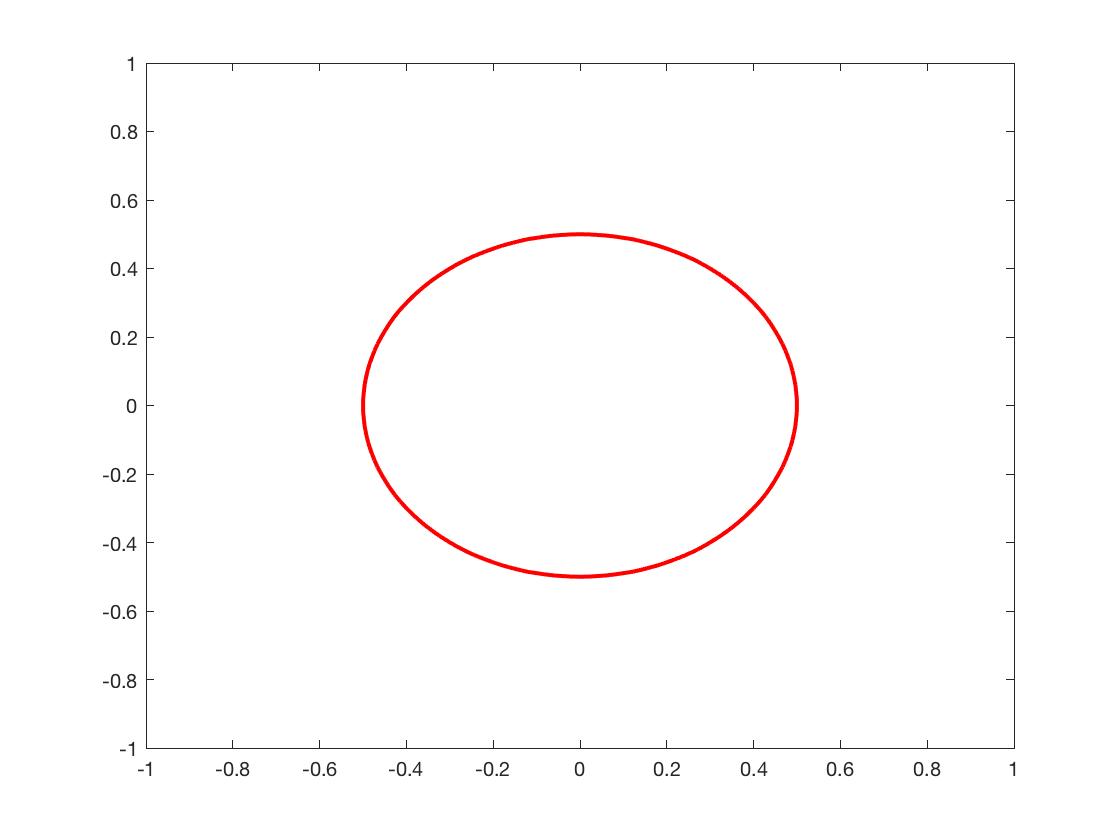
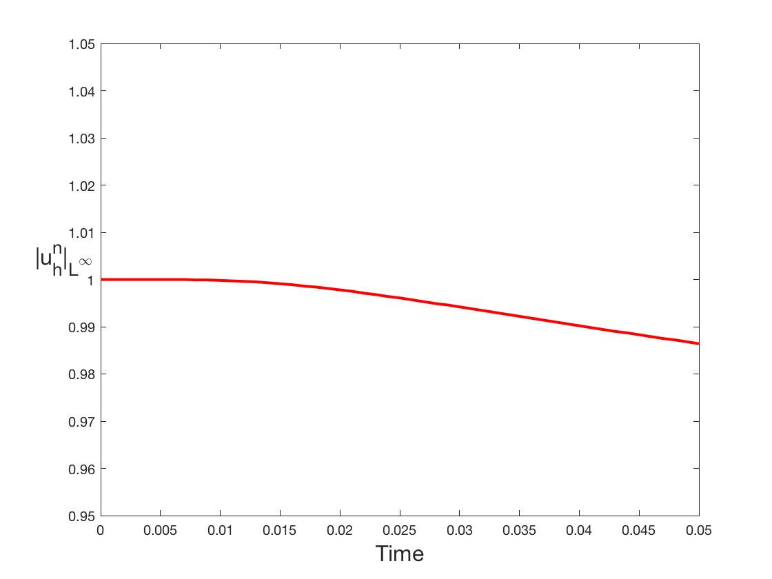
Figure 1: The zero-level set of the initial condition (left) and the $|u_{h}^{n}|_{L^{\infty}}$ bound at different time points (right). In this test, $\epsilon=0.05,\,h=0.04,\,k=0.0001$.

$\mathbf{Test\,2.}$ Consider the Cahn-Hilliard equations (1)-(4) with the following initial condition:

$$u_{0}(x)=\tanh\Bigl{(}\frac{1}{\sqrt{2}\epsilon}\bigl{(}\min\bigl{\{}\sqrt{(x_{1}+0.3)^{2}+x_{2}^{2}}-0.3,\sqrt{(x_{1}-0.3)^{2}+x_{2}^{2}}-0.25\bigr{\}}\bigr{)}\Bigr{)}.$$

Note that $u_{0}$ can be written in the form given in (104) with $d_{0}(x)$ being the signed distance function to the initial curve. We note that $u_{0}$ does not have the desired form as stated in Lemma 1.

Figure 2 plots the zero-level set of this initial condition and $L^{\infty}$ bound $|u_{h}^{n}|_{L^{\infty}}$. We can observe that $|u_{h}^{n}|_{L^{\infty}}\leq 1$, which numerically verifies the assumption (23). In this test, the interaction length $\epsilon=0.025$, the space size $h=0.02$, and the time step size $k=0.0001$.

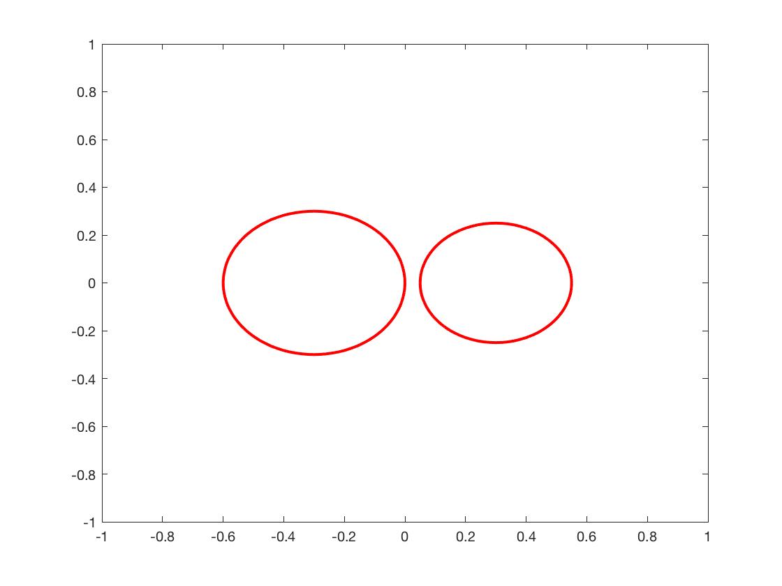
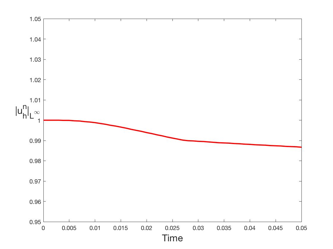
Figure 2: The zero-level set of the initial condition (left) and the $|u_{h}^{n}|_{L^{\infty}}$ bound at different time points (right). In this test, $\epsilon=0.025,\,h=0.02,\,k=0.0001$.

References

- (1) Adams, Robert A and Fournier, John JF, Sobolev spaces, Academic press, 140 (2003)
- (2) Alikakos, Nicholas D and Bates, Peter W and Chen, Xinfu, Convergence of the Cahn-Hilliard equation to the Hele-Shaw model, Arch. Rational Mech. Anal., 128(2), 165–205 (1994)
- (3) Allen, Samuel M and Cahn, John W, A microscopic theory for antiphase boundary motion and its application to antiphase domain coarsening, Acta Metall., 27, 1084–1095 (1979)
- (4) Aristotelous, Andreas C and Karakashian, Ohannes and Wise, Steven M, A mixed Discontinuous Galerkin, Convex Splitting Scheme for a Modified Cahn-Hilliard Equation, Disc. Cont. Dynamic. Syst. Series B., 18(9), 2211–2238 (2013)
- (5) Bartels, Sören and Müller, Rüdiger and Ortner, Christoph, Robust a priori and a posteriori error analysis for the approximation of Allen-Cahn and Ginzburg-Landau equations past topological changes. SIAM Journal on Numerical Analysis, 49(1), 110–134 (2011)
- (6) Bazeley, GP and Cheung, Yo K and Irons, Bo M and Zienkiewicz, OC, Triangular elements in plate bending- conforming and non-conforming solutions(Stiffness characteristics of triangular plate elements in bending, and solutions). 547–576 (1966)
- (7) Riviere, Beatrice, Discontinuous Galerkin methods for solving elliptic and parabolic equations: theory and implementation, SIAM (2008)
- (8) Brenner, Susanne, Two-level additive Schwarz preconditioners for nonconforming finite element methods, Mathematics of Computation of the American Mathematical Society, 65(215), 897–921 (1996)
- (9) Brenner, Susanne, Convergence of nonconforming multigrid methods without full elliptic regularity, Mathematics of Computation of the American Mathematical Society, 68(225), 25–53 (1999)
- (10) Brenner, Susanne C and Sung, Li-yeng and Zhang, Hongchao and Zhang, Yi, A Morley finite element method for the displacement obstacle problem of clamped Kirchhoff plates, Journal of Computational and Applied Mathematics, 254, 31–42 (2013)
- (11) Chen, Xinfu, Spectrum for the Allen-Cahn and Cahn-Hilliard and phase-field equations for generic interfaces, Comm. Partial Diff. Eqs., 19(7-8), 1371–1395 (1994)
- (12) Cheng, Kelong and Feng, Wenqiang and Wang, Cheng and Wise, Steven M, An energy stable fourth order finite difference scheme for the Cahn-Hilliard equation, Journal of Computational and Applied Mathematics, in press, arXiv preprint arXiv:1712.06210 (2017)
- (13) Du, Qiang and Nicolaides, Roy A, Numerical analysis of a continuum model of phase transition, SIAM Journal on Numerical Analysis, 28(5), 1310–1322 (1991)
- (14) Elliott, Charles M and French, Donald A, A nonconforming finite-element method for the two-dimensional Cahn-Hilliard equation, SIAM Journal on Numerical Analysis, 26(4), 884-903 (1989)
- (15) Feng, Xiaobing and Li, Yukun, Analysis of symmetric interior penalty discontinuous Galerkin methods for the Allen–Cahn equation and the mean curvature flow, IMA Journal of Numerical Analysis, 35(4), 1622-1651 (2015)
- (16) Feng, Xiaobing and Li, Yukun and Prohl, Andreas, Finite element approximations of the stochastic mean curvature flow of planar curves of graphs, Stochastic Partial Differential Equations: Analysis and Computations, 2(1), 54–83 (2014)
- (17) Feng, Xiaobing and Li, Yukun and Xing, Yulong, Analysis of Mixed Interior Penalty Discontinuous Galerkin Methods for the Cahn–Hilliard Equation and the Hele–Shaw Flow, SIAM Journal on Numerical Analysis, 54(2), 825–847 (2016)
- (18) Feng, Xiaobing and Li, Yukun and Zhang, Yi, Finite Element Methods for the Stochastic Allen–Cahn Equation with Gradient-type Multiplicative Noise, SIAM Journal on Numerical Analysis, 55(1), 194–216 (2017)
- (19) Feng, Xiaobing and Prohl, Andreas Numerical analysis of the Allen-Cahn equation and approximation for mean curvature flows, Numer. Math., 94, 33–65 (2003)
- (20) Feng, Xiaobing and Prohl, Andreas, Error analysis of a mixed finite element method for the Cahn-Hilliard equation, Numer. Math., 74, 47–84 (2004)
- (21) Feng, Xiaobing and Prohl, Andreas, Numerical analysis of the Cahn-Hilliard equation and approximation for the Hele-Shaw problem, Inter. and Free Bound., 7, 1–28 (2005)
- (22) Feng, Xiaobing and Wu, Hai-jun, A posteriori error estimates and an adaptive finite element method for the Allen–Cahn equation and the mean curvature flow, Journal of Scientific Computing, 24(2), 121–146 (2005)
- (23) Ilmanen, Tom and others, Convergence of the Allen-Cahn equation to Brakke’s motion by mean curvature, J. Diff. Geom., 38(2), 417–461 (1993)
- (24) Kovács, Mihály and Larsson, Stig and Mesforush, Ali, Finite element approximation of the Cahn–Hilliard–Cook equation, SIAM Journal on Numerical Analysis, 49(6), 2407–2429 (2011)
- (25) Lascaux, P and Lesaint, P, Some nonconforming finite elements for the plate bending problem, Revue française d’automatique, informatique, recherche opérationnelle. Analyse numérique, 9(R1), 9–53 (1975)
- (26) Li, Yukun, Numerical Methods for Deterministic and Stochastic Phase Field Models of Phase Transition and Related Geometric Flows, Ph.D. thesis, The University of Tennessee (2015)
- (27) Nilssen, Trygve and Tai, Xue-Cheng and Winther, Ragnar, A robust nonconforming -element, Mathematics of Computation, 70(234), 489–505 (2001)
- (28) Pachpatte, Baburao G, Inequalities for Finite Difference Equations, Chapman & Hall/CRC Pure and Applied Mathematics, 247, CRC Press (2011)
- (29) Stoth, Barbara EE, Convergence of the Cahn-Hilliard equation to the Mullins-Sekerka problem in spherical symmetry, J. Diff. Eqs., 125(1), 154–183 (1996)
- (30) Wang, Ming, On the necessity and sufficiency of the patch test for convergence of nonconforming finite elements, SIAM journal on numerical analysis, 39(2), 363–384 (2001)
- (31) Wang, Ming and Xu, Jinchao, The Morley element for fourth order elliptic equations in any dimensions, Numerische Mathematik, 103(1), 155–169 (2006)
- (32) Wu, Shuonan and Li, Yukun, Analysis of the Morley elements for the Cahn-Hilliard equation and the Hele-Shaw flow, submitted, arXiv preprint arXiv:1808.08581 (2018)
- (33) Xu, Jinchao and Li, Yukun and Wu, Shuonan, Convex splitting schemes interpreted as fully implicit schemes in disguise for phase field modeling, Computer Methods in Applied Mechanics and Engineering, accepted, arXiv preprint arXiv:1604.05402 (2016)