Superconducting Metamaterials

Abstract

Metamaterials, i.e. artificial, man-made media designed to achieve properties not available in natural materials, have been the focus of intense research during the last two decades. Many properties have been discovered and multiple designs have been devised that lead to multiple conceptual and practical applications. Superconducting metamaterials made of superconducting metals have the advantage of ultra low losses, a highly desirable feature. The additional use of the celebrated Josephson effect and SQUID (superconducting quantum interference device) configurations enrich the domain of superconducting metamaterials and produce further specificity and functionality. SQUID-based metamaterials are both theoretically investigated but also fabricated and analyzed experimentally in many laboratories and exciting new phenomena have been found both in the classical and quantum realms. The enticing feature of a SQUID is that it is a unique nonlinear oscillator that can be actually manipulated through multiple external means. This domain flexibility is inherited to SQUID-based metamaterials and metasurfaces, i.e. extended units that contain a large arrangement of SQUIDs in various interaction configurations. Such a unit can be viewed theoretically as an assembly of weakly coupled nonlinear oscillators and as such presents a nonlinear dynamics laboratory where numerous, classical as well as quantum complex, spatio-temporal phenomena may be explored. In this review we focus primarily on SQUID-based superconducting metamaterials and present basic properties related to their individual and collective responses to external drives; the work summarized here is primarily theoretical and computational with nevertheless explicit presentation of recent experimental works. We start by showing how a SQUID-based system acts as a genuine metamaterial with right as well as left handed properties, demonstrate that the intrinsic Josephson nonlinearity leads to wide-band tunability, intrinsic nonlinear as well as flat band localization. We explore further exciting properties such as multistability and self-organization and the emergence of counter-intuitive chimera states of selective, partial organization. We then dwell into the truly quantum regime and explore the interaction of electromagnetic pulses with superconducting qubit units where the coupling between the two yields phenomena such as self-induced transparency and superradiance. We thus attempt to present the rich behavior of coupled superconducting units and point to their basic properties and practical utility.

Contents

		Abstract	1
		Contents	2
1.		Introduction	3
	1.1	Metamaterials $\&$ Synthetic Media: Concepts and Perspectives.	3
	1.2	Nonlinear, Superconducting, and Active Metamaterials.	4
	1.3	Superconducting Metamaterials from Zero to Terahertz Frequencies.	5
	1.4	Summary of Prior Work in Superconducting Metamaterials.	6
	1.5	SQUID Metamaterials.	9
2.		SQUID-Based Metamaterials I: Models and Collective Properties	11
	2.1	The rf-SQUID as an artificial magnetic ”atom”.	11
	2.2	SQUID Metamaterial Models and Flux Wave Dispersion.	18
	2.3	Wide-Band SQUID Metamaterial Tunability with dc Flux.	23
	2.4	Energy Transmission in SQUID Metamaterials.	26
	2.5	Multistability and Self-Organization in Disordered SQUID Metamaterials.	30
3.		SQUID-Based Metamaterials II: Localization and Novel Dynamic States	36
	3.1	Intrinsic Localization in Hamiltonian and Dissipative Systems.	36
	3.2	Dissipative Breathers in SQUID Metamaterials.	36
	3.3	Collective Counter-Intuitive Dynamic States.	39
	3.4	Chimera States in SQUID Metamaterials.	40
		3.4.1           SQUID Metamaterials with Non-Local Coupling.	40
		3.4.2           SQUID Metamaterials with Local Coupling.	46
4.		SQUID Metamaterials on Lieb Lattices.	51
	4.1	Nearest-Neighbor Model and Frequency Spectrum.	51
	4.2	From flat-Band to Nonlinear Localization.	52
5.		Quantum Superconducting Metamaterials.	56
	5.1	Introduction.	56
	5.2	Superconducting Qubits.	57
	5.3	Self-Induced Transparency, Superradiance, and Induced Quantum Coherence.	59
		5.3.1          Description of the Model System.	59
		5.3.2          Second Quantization and Reduction to Maxwell-Bloch Equations.	60
		5.3.3          Approximations and Analytical Solutions.	62
		5.3.4          Numerical Simulations.	64
6.		Summary	69
		Acknowledgements	70
		Appendix: Derivation of the Maxwell-Bloch-sine-Gordon equations.	71
		References	76

1 Introduction

1.1 Metamaterials $\&$ Synthetic Media: Concepts and Perspectives

Metamaterials represent a new class of materials generated by the arrangement of artificial structural elements, designed to achieve advantageous and/or unusual properties that do not occur in natural materials. In particular, naturally occurring materials show a limited range of electrical and magnetic properties, thus restricting our ability to manipulate light and other forms of electromagnetic waves. The functionality of metamaterials, on the other hand, relies on the fact that their constitutive elements can be engineered so that they may achieve access to a widely expanded range of electromagnetic properties. Although metamaterials are often associated with negative refraction, this is only one manifestation of their possible fascinating behaviors; they also demonstrate negative permittivity or permeability, cloaking capabilities ¹, perfect lensing ², high frequency magnetism ³, classical electromagnetically induced transparency ^{4, 5, 6, 7}, as well as dynamic modulation of Terahertz (THz) radiation ⁸, among other properties. High-frequency magnetism, in particular, exhibited by magnetic metamaterials, is considered one of the ”forbidden fruits” in the Tree of Knowledge that has been brought forth by metamaterial research ⁹. Their unique properties allow them to form a material base for other functional devices with tuning and switching capabilities ^{9, 10, 11}. The scientific activity on metamaterials which has exploded since their first experimental demonstration ^{12, 13}, has led to the emergence of a new, rapidly growing interdisciplinary field of science. This field has currently progressed to the point where physicist, material scientists and engineers are now pursuing applications, in a frequency region that spans several orders of magnitude, from zero ^{14, 15, 16, 17, 18} to THz ^{19, 20, 21, 22, 23, 24, 25} and optical ^{3, 26, 27, 28}. Historically, the metamaterial concept goes back to 1967 ²⁹, when V. Veselago investigated hypothetical materials with simultaneously negative permeability and permittivity with respect to their electromagnetic properties. He showed that simultaneously negative permeability and permittivity result in a negative refractive index for such a medium, which would bend the light the ”wrong” way. The realization of materials with simultaneously negative permeability and permittivity, required for negative refractive index, had however to wait until the turn of the century, when D. Smith and his collaborators demonstrated for the first time a structure exhibiting negative refraction in the microwaves ¹². The first metamaterial was fabricated by two interpenetrating subsystems, one them providing negative permittivity while the other negative permeability within the same narrow frequency band. Specifically, an array of thin metallic wires and an array of metallic rings with a slit (split-ring resonators), which were fabricated following the ”recipies” in the seminal works of J. B. Pendry, provided the negative permeability ³⁰ and the negative permittivity ³¹, respectively. The wires and the split-rings act as electrically small resonant ”particles”, undertaking the role of atoms in natural materials; however, they are themselves made of conventional materials (highly conducting metals). Accordingly, a metamaterial represents a higher level of structural organization of matter, which moreover is man-made.

The key element for the construction of metamaterials has customarily been the split-ring resonator (SRR), which is a subwavelength ”particle”; in its simplest version it is just a highly conducting metallic ring with a slit. The SRR and all its subsequent versions, i.e., U particles, H particles, $\Omega$ or $\Omega-$like particles, double and/or multislit SRR molecules, are resonant particles which effectively act as artificial ”magnetic atoms” ³². The SRRs can be regarded as inductive-resistive-capacitive ($RLC$) oscillators, featuring a self-inductance $L$, a capacitance $C$, and a resistance $R$, in an electromagnetic field whose wavelength much larger than their characteristic dimension. As long as a metamaterial comprising SRRs is concerned, the wavelength of the electromagnetic field has to be much larger than its unit cell size; then the field really ”sees” the structure as a homogeneous medium at a macroscopic scale and the macroscopic concepts of permittivity and permeability become meaningful. The (effective) homogeneity is fundamental to the metamaterial concept, as it is the ability to structure a material on a scale less than the wavelength of the electromagnetic field of interest. Although in microwaves this is not a problem, downsizing the scale of metamaterial elements to access the optical frequency range may be a non-trivial issue. The advent of metamaterials has led to structures with many different designs of elemental units and geometries, that may extend to one ^{33, 34}, two ^{13, 17}, or three dimensions ³⁵. One of the most investigated metamaterial designs which does not contain SRRs is the fishnet structure and its versions in two ³⁶, quasi-two ³⁷, and three dimensions ^{38, 39}. However, all these metamaterials have in common that they owe their extraordinary electromagnetic properties more to their carefully designed and constructed internal structure rather than, e.g., chemical composition of their elements. Metamaterials comprising of split-rings or some other variant of resonant elements, are inherently discrete; discreteness effects do not however manifest themselves as long as the metamaterial responds linearly (low-field intensities) and the homogeneous medium approximation holds. The coupling effects, however, in relatively dense SRR metamaterials are of paramount importance for a thorough understanding of certain aspects of their behavior, since they introduce spectral splitting and/or resonant frequency shifts ^{40, 41, 42, 43, 44, 45, 46}. The SRRs are coupled to each other through non-local magnetic and/or electric dipole-dipole interaction, with relative strength depending on the relative orientation of the SRRs in an array. However, due to the nature of the interaction, the coupling energy between neighboring SRRs is already much less than the characteristic energy of the metamaterial; thus in most cases next-nearest and more distant neighbor interactions can be safely neglected. SRR-based metamaterials support a new kind of propagating waves, referred to as magnetoinductive waves, for metamaterials where the magnetic interaction between its units is dominant. They exhibit phonon-like dispersion curves and they can transfer energy ^{33, 47}, and they have been experimentally investigated both in linear and nonlinear SRR-based metamaterials ^{48, 49, 50}. It is thus possible to fabricate contact-free data and power transfer devices which make use of the unique properties of the metamaterial structure, and may function as a frequency-selective communication channel for devices via their magneto-inductive wave modes ⁵¹.

Unfortunately, metamaterials structures comprising of resonant metallic elements revealed unfavorable characteristics that render them unsuitable for most practical applications. The SRRs, in particular, suffer from high Ohmic losses at frequencies close to their resonance, where metamaterials acquire their extraordinary properties. Moreover, those properties may only appear within a very narrow band, that is related to the weak coupling between elements. High losses thus hamper any substantial progress towards the practical use of these metamaterials in novel devices. Many applications are also hampered by the lack of tuning capabilities and relatively bulky size. However, another breakthrough came with the discovery of non-resonant, transmission line negative refractive index metamaterials ^{52, 53}, which very quickly led to several applications, at least in the microwaves ⁵⁴. Transmission line metamaterials rely on the appropriate combination of inductive-capacitive ($L\,C$) lumped elements into large networks. The tremendous amount of activity in the field of metamaterials since $\sim 2000$ has been summarized in various reviews ^{55, 56, 3, 57, 26, 28, 58, 59, 60, 61} and books ^{62, 63, 64, 65, 66, 67, 68, 69, 70, 71, 72, 11}.

1.2 Nonlinear, Superconducting, and Active Metamaterials

Dynamic tunability is a property that is required for applications ⁷³; in principle, one should be able to vary the effective (macroscopic) parameters of a metamaterial in real time, simply by varying an applied field. Tunability provides the means for fabricating meta-devices with switching capabilities ^{9, 10}, among others, and it can be achieved by the introduction of nonlinearity. Nonlinearity adds new degrees of freedom for metamaterial design that allows for both tunability and multistability - another desired property, that may offer altogether new functionalities and electromagnetic characteristics ⁷⁴, as well as wide-band permeability ⁷⁵. It was very soon after the first demonstration of metamaterials, named at that time as negative refractive index materials, when it became clear that the SRR structure has considerable potential to enhance nonlinear effects due to the intense electric fields which can be generated in their slits ⁷⁶. Following these ideas, several research groups have demonstrated nonlinear metamaterial units, by filling the SRR slits with appropriate materials, e.g., with a strongly nonlinear dielectric ⁷⁷, or with a photo-sensitive semiconductor. Other approaches have made use of semiconducting materials, e.g., as substrates, on which the actual metamaterial is fabricated, that enables modulation of THz transmission by $50\%$ ⁷⁸. However, the most convenient method for introducing nonlinearity in SRR-based metamaterials was proved to be the insertion of nonlinear electronic components into the SRR slits, e.g., a variable capacitance diode (varactor) ^{79, 80}. The dynamic tunability of a two-dimensional metamaterial comprising varactor-loaded SRRs by the power of an applied field has been demonstrated experimentally ⁸¹. Both ways of introducing nonlinearity affect the capacitance $C$ of the SRRs which becomes field-dependent; in the equivalent electrical circuit picture, in which the SRRs can be regarded as lumped element electrical oscillators, the capacitance $C$ acquires a voltage dependence and in turn a field-dependent magnetic permeability. Nonlinear transmission line metamaterials are reviewed in Ref. ⁸².

Nonlinearity does not however help in the reduction of losses; in nonlinear metamaterials the losses continue to be a serious problem. The quest for loss compensation in metamaterials is currently following two different pathways: a ”passive” one, where the metallic elements are replaced by superconducting ones ^{58, 83}, and an ”active” one, where appropriate constituents are added to metallic metamaterials that provide gain through external energy sources. In order to fabricate both nonlinear and active metamaterials, gain-providing electronic components such as tunnel (Esaki) diodes ⁸⁴ or particular combinations of other gain-providing devices have to be utilized. The Esaki diode, in particular, features a negative resistance part in its current-voltage characteristics, and therefore can provide both gain and nonlinearity in a conventional (i.e., metallic) metamaterial. Tunnel diodes which are biased so that they operate at the negative resistance region of their characteristics may also be employed for the construction of ${\cal PT}-$symmetric metamaterials, that rely on balanced gain and loss ⁸⁵. ${\cal PT}-$symmetric systems correspond to a new paradigm in the realm of artificial or ”synthetic” materials that do not obey separately the parity ($\cal P$) and time ($\cal T$) symmetries; instead, they do exhibit a combined ${\cal PT}$ symmetry ^{86, 87}. The notions of ${\cal PT}-$symmetric systems originate for non-Hermitian quantum mechanics ^{88, 89}, but they have been recently extended to optical lattices ^{90, 91}. The use of active components which are incorporated in metamaterial unit elements has been actually proposed several years ago ⁹², and it is currently recognized as a very promising technique of compensating losses ⁹³. Low-loss and active negative index metamaterials by incorporating gain material in areas with high local field have been demonstrated in the optical ⁹⁴. Recently, transmission lines with periodically loaded tunnel diodes which have the negative differential resistance property have been realized and tested as low-loss metamaterials, in which intrinsic losses are compensated by gain ⁹⁵. Moreover, a combination of transistors and a split-ring has been shown to act as a loss-compensated metamaterial element ⁹⁶. In the latter experiment, the quality factor for the combined system exhibits huge enhancement compared with that measured for the split-ring alone.

The ”passive” approach to loss reduction employes superconducting materials, i.e, materials exhibiting absence of dc resistance below a particular temperature, known as the critical temperature, $T_{c}$. A rough classification of the superconducting materials is made on the basis of their critical temperature; according to that, there are low-$T_{c}$ and high-$T_{c}$ superconducting materials. The former include primarily elemental and binary compounds, like Niobium (Nb), Niobium di-Selenide (NbSe₂) and more recently Niobium Nitride (NbN), while the most known representatives of the latter are the superconducting perovskites such as Yttrium-Barium-Copper-Oxide (YBCO). The latter is the most commonly used perovskite superconductor which typically has a critical temperature $T_{c}\sim 90K$, well above the boiling point of liquid Nitrogen. The last few years, there has been an increasing interest in superconducting metamaterials that exploit the zero resistance property of superconductivity, targeting at severe reduction of losses and the emergence of intrinsic nonlinearities due to the extreme sensitivity of the superconducting state to external stimuli ^{10, 58}. The direct approach towards fabrication of superconducting metamaterials relies on the replacement of the metallic split-rings of the conventional SRR-based metamaterials by superconducting ones. More shopisticated realizations of superconducting metamaterials result from the replacement of the metallic SRRs by rf SQUIDs (Superconducting QUantum Interference Devices) ⁹⁷; those SQUID metamaterials are discussed below.

Superconducting metamaterials are not however limited to the above mentioned realizations, but they also include other types of artificial metamaterials; thin superconducting plates have been used in a particular geometrical arrangement to ”beat the static” ⁹⁸ and make possible a zero frequency metamaterial (dc metamaterial) ^{14, 15, 16, 99, 17}. Other types of superconducting metamaterials in the form of heterostructures, where superconducting layers alternate with ferromagnetic or non-magnetic metallic layers have been shown to exhibit electromagnetically induced transparency ^{5, 100, 6}, switching capabilities ¹⁰¹, magnetic cloaking, and concentration ¹⁰². Recently, tunable electromagnetically induced transparency has been demonstrated in a Niobium Nitride (NbN) terahertz (THz) superconducting metamaterial. An intense THz pulse is used to induce nonlinearities in the NbN thin film and thereby tune the electromagnetically induced transparency-like behavior ⁷. Furthermore, the dynamic process of parity-time ($\cal PT$) symmetry breaking was experimentally demonstrated in a hybridized metasurface which consists of two coupled resonators made from metal and NbN ¹⁰³. Negative refraction index metamaterials in the visible spectrum, based on MgB₂/SiC composites, have been also realized ¹⁰⁴, following prior theoretical investigations ¹⁰⁵. Moreover, there is substantial evidence for negative refraction index in layered superconductors above the plasma frequency of the Josephson plasma waves ¹⁰⁶, that was theoretically investigated by several authors ^{107, 108}. Other types of superconducting metamaterials include those made of magnetically active planar spirals ¹⁰⁹, as well as those with rather special (”woodcut”) geometries ¹¹⁰, two-dimensional arrays of Josephson junctions ¹¹¹, as well as superconducting ”left-handed” transmission lines ^{112, 113}. Recently, in a novel one-dimensional Josephson metamaterial composed of a chain of asymmetric SQUIDs, strong Kerr nonlinearity was demonstrated ¹¹⁴. Moreover, the Kerr constant was tunable over a wide range, from positive to negative values, by a magnetic flux threading the SQUIDs.

1.3 Superconducting Metamaterials from Zero to Terahertz Frequencies

There are several demonstrations of superconducting metamaterial elements which exhibit tunability of their properties by varying the temperature or the applied magnetic field ^{115, 116, 22, 117, 24, 118, 119}. We should also mention the theoretical investigations (nonlinear circuit modeling) on a multi-resonant superconducting split-ring resonator ¹²⁰, and on a ”meta-atom” composed of a direct current (dc) SQUID and a superconducting rod attached to it, which exhibits both electric and magnetic resonant response ¹²¹. Superconducting split-rings combined into two-dimensional planar arrays form superconducting metamaterials exhibiting tunability and switching capabilities at microwave and THz frequencies ^{22, 116, 122, 23, 24, 123, 124, 125, 126, 25, 127}. Up to the time of writing, metamaterials comprising superconducting SRRs employ one of the following geometries:

(i) square SRRs with rectangular cross-section in the double, narrow-side coupled SRR geometry ^{115, 128, 116};

(ii) circular, asymmetrically split-rings ^{117, 129, 130};

(iii) square SRRs with rectangular cross-section in the single SRR geometry ²²;

(iv) electric inductive-capacitive SRRs of two different types ¹³¹.

Also, novel metamaterial designs including a ”woodcut” type superconducting metamaterial, and niobium-connected asymmetrically split-ring metamaterials were demonstrated ¹³⁰. All these metamaterials were fabricated in the planar geometry, using either conventional, low$-T_{c}$ superconductors such as niobium (Nb) and niobium nitride films, or the most widely used member of the high$-T_{c}$ superconductor family, i.e., the yttrium-barium-copper-oxide ($YBCO$). The experiments were performed in microwaves and in the (sub-)THz range ($\sim 0.1-2~{}THz$).

All these superconducting metamaterials share a common feature: they all comprise resonant sub-wavelength superconducting elements, that exhibit a strong response at one particular frequency, i.e., the resonance frequency, $f_{0}$. That resonance frequency is tunable under external fields, such as temperature, constant (dc) and time-periodic (ac) magnetic fields, and applied current, due to the extreme sensitivity of the superconducting state to external stimuli. (Note however that for some geometries there can be more than one strong resonances.) The experimental investigation of the resonances and their ability for being shifted either to higher or lower frequencies relies on measurements of the complex transmission spectrums, with dips signifying the existence of resonances. However, not only the frequency of a resonance but also its quality is of great interest in prospective applications. That quality is indicated by the depth of the dip of the complex transmission magnitude in the corresponding transmission spectrum, as well as its width, and quantified by the corresponding quality factor $Q$. In general, the quality factor increases considerably as the temperature decreases below the critical one at $T_{c}$. Other factors, related to the geometry and material issues of the superconducting SRRs that comprise the metamaterial, also affect the resonance frequency $f_{0}$. Thus, the resonance properties of a metamaterial can be engineered to achieve the desired values, just like in conventional metamaterials. However, for superconducting metamaterials, the thickness of the superconducting film seems to be an important parameter, because of the peculiar magnetic properties of superconductors. Using proper design, it is possible to switch on and off the resonance in superconducting metamaterials in very short time-scales, providing thus the means of manufacturing devices with fast switching capabilities.

1.4 Summary of earlier work in superconducting metamaterials

In this Subsection, a brief account is given on the progress in the development and applications of superconducting (both classical and quantum) metamaterials, i.e., metamaterials utilizing either superconducting materials or devices, is given. A more detailed and extended account is given in two review articles on the subject ^{58, 83}, as well as in Chapter $5.5$ of a recently published book ¹¹. The status of the current research on SQUID metamaterials is discussed separately in the next Subsection (Subsection $1.5$). In the older of the two review articles ⁵⁸, the properties of superconductors which are relevant to superconducting metamaterials, and the advantages of superconducting metamaterials over their normal metal counterparts are discussed. The author reviews the status of superconductor-ferromagnet composites, dc superconducting metamaterials, radio frequency (rf) superconducting metamaterials, and superconducting photonic crystals (although the latter fall outside the domain of what are usually called metamaterials). There is also a brief discussion on SQUID metamaterials, with reference to the theoretical works in which it was proposed to use an array of rf SQUIDs as a metamaterial ^{132, 133}. In the second review article ⁸³, a more detailed account on the advantages of superconducting metamaterials over their normal metal counterparts was given, along with an update on the status of superconducting metamaterials. Moreover, analogue electromagnetically-induced transparency superconducting metamaterials and superconducting SRR-based metamaterials are also reviewed. In this review article, there is also a discussion on the first experiments on SQUID metamaterials ^{34, 134, 135} which have confirmed earlier theoretical predictions. However, a lot of experimental and theoretical work on SQUID metamaterials has been performed after the time of writing of the second review article in this field. The present review article aims to give an up-to-date and extended account of the theoretical and experimental work on SQUID metamaterials and reveal their extraordinary nonlinear dynamic properties. SQUID metamaterials provide a unique testbed for exploring complex spatio-temporal dynamics. In the quantum regime, a prototype model for a ”basic” SCQMM which has been investigated by several authors is reviewed, which exhibits novel physical properties. Some of these properties are discussed in detail.

Superconductivity is a macroscopic quantum state of matter which arises from the interaction between electrons and lattice vibrations; as a results, the electrons form pairs (Cooper pairs) which condense into a single macroscopic ground state. The latter is the equilibrium thermodynamic state below a transition (critical) temperature $T_{c}$. The ground state is separated by a temperature-dependent energy gap $\Delta$ from the excited states with quasi-particles (quasi-electrons). As mentioned earlier, the superconductors are roughly classified into high and low critical temperature ones (high$-T_{c}$ and low$-T_{c}$, respectively). In some circumstances, the Cooper pairs can be described in terms of a single macroscopic quantum wavefunction $\Psi=\sqrt{n_{s}}\,\exp[i\theta_{s}]$, whose squared magnitude is interpreted as the local density of superconducting electrons ($n_{s}$), and whose phase $\theta_{s}$ is coherent over macroscopic dimensions. Superconductivity exhibits several extraordinary properties, such as zero dc resistance and the Meissner effect. Importantly, it also exhibits macroscopic quantum phenomena including fluxoid quantization and the Josephson effects at tunnel (insulating) barriers and weak links. When two superconductors $S_{L}$ and $S_{R}$ are brought close together and separated by a thin insulating barrier, there can be tunneling of Cooper pairs from one superconductor to the other. This tunneling produces a supercurrent (Josephson current) between $S_{L}$ and $S_{R}$, $I_{J}=I_{c}\,\sin(\phi_{J})$, where $I_{c}$ is the critical current of the Josephson junction and $\phi_{J}=\phi_{L}(t)-\phi_{R}(t)-\frac{2\pi}{\Phi_{0}}\int_{S_{L}}^{S_{R}}{\bf A}({\bf r},t)d{\bf l}$ is the gauge-invariant Josephson phase, with $\phi_{L}$ and $\phi_{R}$ being the phases of the macroscopic quantum wavefunctions of $S_{L}$ and $S_{R}$, respectively, ${\bf A}({\bf r},t)$ the electromagnetic vector potential in the region between $S_{L}$ and $S_{R}$, and $\Phi_{0}=\frac{h}{2e}\simeq 2.07\times 10^{-15}~{}Wb$ the flux quantum ($h$ is Planck’s constant and $e$ the electron’s charge). Depending on whether $\phi_{J}$ is time-dependent or not, the appearance of the supercurrent $I_{J}$ is referred to as the ac or the dc Josephson effect.

Superconductors bring three unique advantages to the development of metamaterials in the microwave and sub-THz frequencies which have been analyzed in Refs. ^{58, 83}. Namely, (i) low losses (one of the key limitations of conventional metamaterials), (ii) the possibility for higher compactification of superconducting metamaterials compared to other realizations (superconducting SRRs can be substantially miniaturized while still maintaining their low-loss properties), and (iii) strong nonlinearities inherent to the superconducting state, which allow for tunability and provide switching capabilities. The limitations of superconducting metamaterials arise from the need to create and maintain a cryogenic environment, and to bring signals to and from the surrounding room temperature environment. Quite fortunately, closed-cycle cryocoolers have become remarkably small, efficient and inexpensive since the discovery of high$-T_{c}$ superconductors, so that they are now able to operate for several years unattended, and moreover they can accommodate the heat load associated with microwave input and output transmission lines to room temperature. Superconductors can also be very sensitive to variations in temperature, stray magnetic field, or strong rf power which can alter their properties and change the behavior of the metamaterial. Thus, careful temperature control and high quality magnetic shielding are often required for reliable performance of superconducting metamaterials.

Superconducting metamaterials exhibit intrinsic nonlinearity because they are typically made up of very compact elementary units, resulting in strong currents and fields within them. Nonlinearity provides tunability through the variation of external fields. For example, a connected array of asymmetrically-split Nb resonators shows transmission tunable by current at sub-THz frequencies due to localized heating and the entrance of magnetic vortices ¹²⁹. The change in superfluid density by a change in temperature was demonstrated for a superconducting thin film SRR ¹²⁸. Later, it was demonstrated that the resonant frequency of a Nb SRR changes significantly with the entry of magnetic vortices ¹¹⁶. Similar results showing complex tuning with magnetic field were later demonstrated at microwaves using high$-T_{c}$ superconducting SRRs ¹¹⁹ and at sub-THz frequencies with similarly designed Nb SRRs ¹³⁰. The nonlinearity associated with the resistive transition of the superconductor was exploited to demonstrate a bolometric detector at sub-THz frequencies using the collective properties of an asymmetrically split-ring array made of Nb ¹³⁰. Thermal tuning has been accomplished at THz frequencies by varying the temperature in high$-T_{c}$ (YBCO) metamaterial ²⁴ and NbN electric inductive-capacitive thin film resonators ¹²⁴. Enchancement of thermal tunability was accomplished by decreasing the thickness of the high$-T_{c}$ superconducting films which make up square SRRs ¹³⁶. Fast nonlinear response can be obtained in superconducting films in THz time-domain experiments. In such an experiment it was found that intense THz pulses on a NbN metamaterial could break significant number of Cooper pairs to produce a large quasi-particle density which increases the effective surface resistance of the film and modulates the depth of the SRR resonance ^{25, 126}. The tuning of high$-T_{c}$ (YBCO) SRR metamaterial with variable THz beam intensity has demonstrated that the resonance strength decreases and the resonance frequency shifts as the intensity is increased ¹²⁷.

A natural opportunity to create a negative real part of the effective magnetic permeability $\mu_{eff}$ is offered by a gyromagnetic material for frequencies above the ferromagnetic resonance ¹³⁷. However, the imaginary part of $\mu_{eff}$ is quite large near the resonance and limits the utility of such a metamaterial. A hybrid metamaterial, resulting from the combination of the gyromagnetic material mentioned earlier with a superconductor can help to reduce losses ¹³⁸. A superlattice consisting of high$-T_{c}$ superconducting and manganite ferromagnetic layers (YBCO/LSMO) was created and it was shown to produce a negative index band in the vicinity of the ferromagnetic resonance ($\sim 90~{}GHz$) at magnetic fields between $2.9$ and $3.1~{}T$ ¹⁰⁷. More recently, a metamaterial composed of permanent magnetic ferrite rods and metallic wires was fabricated. This metamaterial exhibits not only negative refraction but also near-zero refraction, without external magnetic field ¹³⁹.

The concept of a dc metamaterial operating at very low frequencies that could make up a dc magnetic cloak has been proposed and investigated in Ref. ¹⁴. The first realization of such a metamaterial, which is based on non-resonant elements, consists of an array of superconducting plates ¹⁵. The superconducting elements exclude a static magnetic field, and provide the foundation for the diamagnetic effect, when that field is applied normal to the plates. The strength of the response depends on the ratio between the dimension of the plates and the lattice spacing. An experimental demonstration of a dc metamaterial cloak was made using an arrangement of Pb thin film plates ¹⁵. Subsequent theoretical work has refined the dc magnetic cloak design and suggested that it can be implemented with high$-T_{c}$ superconducting thin films ¹⁶. It was later demonstrated experimentally that a specially designed cylindrical superconductor-ferromagnet bilayer can exactly cloak uniform static magnetic fields ⁹⁹.

Superconducting rf metamaterials consisting of two-dimensional Nb spirals developed on quartz substrates show strong tunability as the transition temperature is approached ^{122, 109}. Rf metamaterials have great potential in applications such as magnetic resonance imaging devices for non-invasive and high resolution medical imaging ¹⁴⁰. The superconducting rf metamaterials have many advantages over their normal metal counterparts, such as reducing considerably the Ohmic losses, compact structure, and sensitive tuning of resonances with temperature or rf magnetic field, which makes them promising for rf applications. Similar, high$-T_{c}$ rf metamaterials (in which the spirals are made by YBCO) were also fabricated, which enable higher operating temperatures and greater tunability ¹⁴¹.

The elementary units (i.e., the meta-atoms) in a metamaterial can be combined into meta-molecules so that the interactions between the meta-atoms can give rise to qualitatively new effects, such as the classical analogue of the electromagnetically induced transparency (EIT). This effect has been observed in asymmetrically-split ring metamaterials in which Fano resonances have been measured as peaks in the transmission spectrum, corresponding to metamaterial induced transparency ¹¹⁷. Metamaterials consisting of normal metal - superconductor hybrid meta-molecules can create strong classical EIT effects ⁵. The meta-molecule consists of a gold (Au) strip with end caps and two superconducting (Nb) SRRs (the ”bright” and the ”dark” element, respectively). A tunable transparency window which could even be switched off completely by increasing the intensity of the signal propagating through the meta-molecule was demonstrated ^{5, 101}. EIT effects were also observed in the THz domain utilizing NbN bright and dark resonators to create a transparency window ¹⁰⁰. Further experiments on all-superconducting (NbN) metamaterials utilizing strongly coupled SRR-superconducting ring elements showed enhanced slow-light features ⁶.

A quantum metamaterial is meant to be an artificial optical medium that (a) comprise quantum coherent unit elements whose parameters can be tailored, (b) the quantum states of (at least some of) these elements can be directly controlled, and (c) maintain global coherence for sufficiently long time. These properties make a quantum metamaterial a qualitatively different system ^{142, 143}. Superconducting quantum metamaterials offer nowadays a wide range of prospects from detecting single microwave photons to quantum birefringence and superradiant phase transitions ⁸³. They may also play a role in quantum computing and quantum memories. The last few years, novel superconducting devices, which can be coupled strongly to external electromagnetic field, can serve as the quantum coherent unit elements of superconducting quantum metamaterials (SCQMMs). For example, at ultra-low temperatures, superconducting loops containing Josephson junctions exhibit a discrete energy level spectrum and thus behave in many aspects as quantum meta-atoms. It is very common to approximate such devices as two-level quantum systems, referred to as superconducting qubits, whose energy level splitting corresponds to a frequency of the order of a few GHz. The interaction between light and a SCQMM is described by photons coupling to the artificial two-level systems, i.e., the superconducting qubits. The condition of keeping the energy of thermal fluctuations $k_{B}\,T$, where $k_{B}$ is Boltzmann’s constant and $T$ the temperature, below the energy level splitting $h\,f$ of the qubit, where $h$ is Planck’s constant and $f$ the transition frequency, requires temperatures well below $1~{}K$. In the past few years, research on superconducting qubits has made enormous progress that paves the way towards superconducting qubit-based quantum metamaterials.

There are several theoretical investigations on the physics of one-dimensional arrays of superconducting qubits coupled to transmission-line resonators ^{144, 145, 146, 147, 148, 149, 150, 151, 152}. Moreover, two-dimensional ¹⁵³ and three-dimensional ³⁵ SCQMMs based on Josephson junction networks were proposed. A more extended discussion of the theoretical works on SCQMMs is given in Subsection $5.1$. Still there is little progress in the experimental realization of such systems. The first SCQMM which was implemented in 2014 ¹⁵⁴, and comprises $20$ flux qubits arranged in a double chain geometry. In that prototype system, the dispersive shift of the resonator frequency imposed by the SCQMM was observed. Moreover, the collective resonant coupling of groups of qubits with the quantized mode of a photon field was identified, despite of the relatively large spread of the qubit parameters. Recently, an experiment on an SCQMM comprising an array of $15$ twin flux qubits, was demonstrated ¹⁵⁵. The qubit array is embedded directly into the central electrode of an Al coplanar waveguide; each qubit contains $5$ Josephson junctions, and it is strongly coupled to the electromagnetic waves propagating through the system. It was observed that in a broad frequency range, the transmission coefficient through that SCQMM depends periodically on the external magnetic field. Moreover, the excitation of the qubits in the array leads to a large resonant enhancement of the transmission. We undoubtedly expect to see more experiments with arrays of superconducting qubits placed in transmission lines or waveguides in the near future.

1.5 SQUID Metamaterials

The rf SQUIDs, mentioned above, are highly nonlinear superconducting devices which are long known in the Josephson community and encompass the Josephson effect ¹⁵⁶. The simplest version of a SQUID is made by a superconducting ring which is interrupted by a Josephson junction (JJ); the latter is typically formed by two superconductors separated by a thin insulating (dielectric) layer. The current through the insulating layer and the voltage across the junction are then determined by the celebrated Josephson relations and crucially affect the electromagnetic behavior of the rf SQUID. SQUIDs have found numerous technological applications in modern science ^{157, 158, 159, 160}; they are most commonly used as magnetic field sensors, since they can detect even tiny magnetic fields and measure their intensity with unprecedented precision. SQUID metamaterials constitute the direct superconducting analogue of conventional (metallic) nonlinear (i.e., varactor loaded) SRR-based magnetic metamaterials, which result from the replacement of the nonlinear SRRs by rf SQUIDs. The latter possess inherent nonlinearity due to the Josephson element. Similarly to the conventional (metallic), SRR-based magnetic metamaterials, the SQUIDs are coupled magnetically to each other through magnetic dipole-dipole interactions. Several years ago, theoretical investigations have suggested that rf SQUID arrays in one and two dimensions can operate as magnetic metamaterials both in the classical ¹³³ and in the quantum regime ¹³², and they may exhibit negative and/or oscillating effective magnetic permeability in a particular frequency band which encloses the resonance frequency of individual SQUIDs. Recent experiments on single rf SQUIDs in a waveguide demonstrated directly the feasibility of constructing SQUID-based thin-film metasurfaces ¹¹⁸. Subsequent experiments on one-dimensional, quasi-two-dimensional, and truly two-dimensional SQUID metamaterials have revealed a number of several extraordinary properties such as negative diamagnetic permeability ^{118, 34}, broad-band tunability ^{34, 134}, self-induced broad-band transparency ¹⁶¹, dynamic multistability and switching ¹³⁵, as well as coherent oscillations ¹⁶². Moreover, nonlinear localization ¹⁶³ and nonlinear band-opening (nonlinear transmission) ¹⁶⁴, as well as the emergence of dynamic states referred to as chimera states in current literature ^{165, 166}, have been demonstrated numerically in SQUID metamaterial models. Those counter-intuitive dynamic states, which have been discovered numerically in rings of identical phase oscillators ¹⁶⁷, are reviewed in Refs. ^{168, 169}. Moreover, numerical investigations on SQUID metamaterials on Lieb lattices which posses a flat band in their frequency spectrum, reveal the existence of flat-band localized states in the linear regime and the more well-known nonlinearly localized states in the nonlinear regime ¹⁷⁰. The interaction of an electromagnetic wave with a diluted concentration of a chain of SQUIDs in a thin film suggests a mechanism for the excitation of magnetization waves along the chain by a normally incident field ¹⁷¹. In the linear limit, a two-dimensional array of rf SQUIDs acts as a metasurface that controls the polarization of an electromagnetic wave ¹⁷².

SQUID arrays have been also integrated in larger devices in order to take advantage of their extraordinary properties; notably, amplification and squeezing of quantum noise has been recently achieved with a tunable SQUID-based metamaterial ¹⁷³. Other important developments demonstrate clearly that SQUID-based metamaterials enable feedback control of superconducting cubits ¹⁷⁴, observation of Casimir effects ¹⁷⁵, measurements of nanomechanical motion below the standard quantum limit ¹⁷⁶, and three-wave mixing ¹⁷⁷. At sufficiently low (sub-Kelvin) temperatures, SQUID metamaterials provide access to the quantum regime, where rf SQUIDs can be manipulated as flux and phase qubits ^{178, 179}. Recently, the technological advances that led to nano-SQUIDs make possible the fabrication of SQUID metamaterials at the nanoscale ¹⁸⁰.

From the above discussion it should be clear that the field of superconducting metamaterials, in which superconductivity plays a substantial role in determining their properties, has expanded substantially. In this review, we focus on the SQUID metamaterials, that represent an area of the field of superconducting metamaterials, which however has already reached a level of maturity. We also focus on SCQMMs, and in particular on a prototype model for a chain of charge qubits in a transmission-line resonator ¹⁴⁴. The SCQMMs are related to the (classical, i.e., not truly quantum) SQUID metamaterials in that they also encompass the Josephson effect. In Section 2, we describe the SQUID metamaterial models used for simulating real systems in current research, we provide the corresponding dispersion of flux waves which can propagate in SQUID metamaterials, and we present numerical results (along with selected experimental ones), which reveal novel properties such as wide-band tunability, energy transmission, and multistability. In Section 3, we present and discuss results on nonlinear localization in SQUID metamaterials, which leads to the generation of states referred to as discrete breathers. In that Section, we also emphasize the possibility for the emergence of chimera states in SQUID metamaterial models with either nonlocal or local (nearest-neighbor) couplng between their elements (i.e., the SQUIDs). In Section 4, the dynamical model for SQUID metamaterials on a Lieb lattice is presented, along with its full frequency spectrum. The latter contains a flat band, which allows for the formation of flat-band localized states in the linear regime. The case of nonlinearly localized states, which can be formed in the nonlinear regime, as well as the transition between the two regimes, is investigated. In Section 5, we describe a model SCQMMs (a chain of charge qubits in a superconducting transmission-line resonator) and discuss the possibility for having propagating self-induced transparent or superradiant pulses in that medium. Most importantly, those pulses induce quantum coherence effects in the medium itself, by exciting population inversion pulses in the qubit subsystem. Moreover, the speed of the propagating pulses can be controlled by proper engineering of the parameters of the qubits. The most important points made in this review are summarized in Section 6.

2 SQUID-Based Metamaterials I: Models and Collective Properties

2.1 The rf-SQUID as an artificial magnetic ”atom”

The Superconducting QUantum Interference Device (SQUID) is currently one of the most important solid-state circuit elements for superconducting electronics ¹⁸¹; among many other technological applications ^{157, 159, 160}, SQUIDs are used in devices that provide the most sensitive sensors of magnetic fields. Recent advances that led to nano-SQUIDs ¹⁸⁰ makes the fabrication of SQUID metamaterials at the nanoscale an interesting possibility. The radio-frequency (rf) SQUID, in particular, shown schematically in Fig. 1(a), consists of a superconducting ring of self-inductance $L$ interrupted by a Josephson junction (JJ) ¹⁵⁶. A JJ is made by two superconductors connected through a ”weak link”, i.e., through a region of weakened superconductivity. A common type of a JJ is usually fabricated by two superconductors separated by a thin dielectric oxide layer (insulating barrier) as shown in Fig. 2(a); such a JJ is referred to as a superconductor-insulator-superconductor (SIS) junction. The fundamental properties of JJs have been established long ago ^{182, 97}, and their usage in applications involving superconducting circuits has been thoroughly explored. The observed Josephson effect in such a junction, has been predicted by Brian D. Josephson in 1962 and it is of great importance in the field of superconductivity as well as in physics. That effect has been exploited in numerous applications in superconducting electronics, sensors, and high frequency devices. In an ideal JJ, whose electrical circuit symbol is shown in Fig. 2(b), the (super)current (Josephson current) $I_{J}$ through the JJ and the voltage $V_{J}$ across the JJ are related through the celebrated Josephson relations ¹⁵⁶

$$V_{J}(t)=\frac{\Phi_{0}}{2\pi}\frac{\partial\phi_{J}(t)}{\partial t},\qquad I_{J}(t)=I_{c}\,\sin[\phi_{J}(t)],$$ (1)

where $I_{c}$ is the critical current of the JJ, $\Phi_{0}=\frac{h}{2e}\simeq 2.07\times 10^{-15}~{}Wb$ is the flux quantum, with with $h$ and $e$ being the Planck’s constant and the electron’s charge, respectively, and $\phi_{J}$ is the difference of the phases of the order parameters of the superconductors at left ($S_{L}$) and right ($S_{R}$) of the barrier $\phi_{L}$ and $\phi_{R}$, respectively (Fig. 2(a)), i.e., $\phi_{J}=\phi_{L}-\phi_{R}$ (the Josephson phase). In the presence of an electromagnetic potential ${\bf A}({\bf r},t)$, the corresponding gauge-invariant Josephson phase is

$$\phi_{J}(t)=\phi_{L}(t)-\phi_{R}(t)-\frac{2\pi}{\Phi_{0}}\int_{S_{L}}^{S_{R}}{\bf A}({\bf r},t)d{\bf l}.$$ (2)

In an ideal JJ, in which the (super)current is carried solely by Cooper pairs, there is no voltage drop across the barrier of the JJ. In practice, however, this can only be true at zero temperature ($T=0$), while at finite temperatures there will always be a quasi-partice current. The latter is carried single-electron excitations (quasi-electrons) resulting from thermal breaking of Cooper pairs due to the non-zero temperature, and it is subjected to losses. In superconducting circuits, a real JJ is often considered as the parallel combination of an ideal JJ (described by Eqs. (1)), a shunting capacitance $C$, due to the thin insulating layer, and a shunting resistance $R$, due to quasi-electron tunneling through the insulating barrier, i.e., the quasi-particle current (Fig. 2(c)). This equivalent electrical circuit for a real JJ is known as the Resistively and Capacitively Shunted Junction (RCSJ) model, and is widely used for modeling SIS Josephson junctions. The ideal JJ can be also described as a variable inductor, in a superconducting circuit. From the Josephson relations Eqs. (1) and the current-voltage relation for an ordinary inductor $U=L(\partial I/\partial t)$, it is easily deduced that the Josephson inductance is

$$L\equiv L_{J}\equiv L_{J}(\phi_{J})=\frac{L_{J}(0)}{\cos(\phi_{J})},\qquad L_{J}(0)=\frac{\Phi_{0}}{2\pi I_{c}}.$$ (3)

Note that Eq. (3) describes a nonlinear inductance, since $L_{J}$ depends both on the current and the voltage through the Josephson phase $\phi_{J}$.

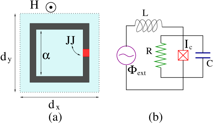
Figure 1: (a) Schematic drawing of an rf SQUID in a time-dependent magnetic field ${\bf H}(t)$ perpendicular to its loop. (b) Equivalent electrical circuit for an rf SQUID driven by a time-dependent flux source $\Phi_{ext}(t)$.

Due to the Josephson element (i.e., the JJ), the rf SQUID is a highly nonlinear oscillator that responds in a manner analogous to a magnetic ”atom”, exhibiting strong resonance in a time-varying magnetic field with appropriate polarization. Moreover, it exhibits very rich dynamic behavior, including chaotic effects ^{183, 184, 185} and tunability of its resonance frequency with external fields ¹⁸⁶. The equivalent electrical circuit for an rf SQUID in a time-dependent magnetic field ${\bf H}(t)$ threading perpendicularly its loop, as shown schematically in Fig. 1(b), comprises a flux source $\Phi_{ext}(t)$ in series with an inductance $L$ and a real JJ described by the RCSJ model.

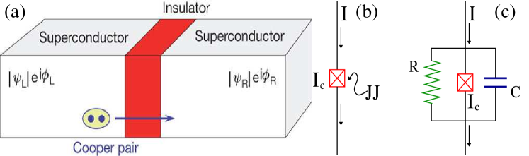
Figure 2: (a) Schematic of a superconductor-insulator-superconductor (SIS) Josephson junction that consists of two superconducting plates separated by a thin insulating layer. Cooper pairs can tunnel through the barrier without loss of energy. The order parameters of the left and right superconductors are $|\Psi_{L}|\exp(i\Phi_{L})$ and $|\Psi_{R}|\exp(i\Phi_{R})$, respectively. (b) The electrical circuit symbol of a Josephson junction. (c) The equivalent circuit of a real Josephson junction according to the widely used Resistively and Capacitively Shunted (RCSJ) junction model.

The dynamic equation for the flux $\Phi$ threading the loop of the rf SQUID is obtained by direct application of Kirchhoff’s laws, as

$$C\frac{d^{2}\Phi}{dt^{2}}+\frac{1}{R}\frac{d\Phi}{dt}+I_{c}\,\sin\left(2\pi\frac{\Phi}{\Phi_{0}}\right)+\frac{\Phi-\Phi_{ext}}{L}=0,$$ (4)

where $\Phi_{0}$ is the magnetic flux quantum, $I_{c}$ is the critical current of the JJ, and $t$ is the temporal variable. Eq. (4) is derived from the combination of the single-SQUID flux-balance relation

$$\Phi=\Phi_{ext}+L\,I,$$ (5)

and the expression for the current in the SQUID $I$ provided by the RCSJ model

$$-I=+C\frac{d^{2}\Phi}{dt^{2}}+\frac{1}{R}\frac{d\Phi}{dt}+I_{c}\,\sin\left(2\pi\frac{\Phi}{\Phi_{0}}\right).$$ (6)

Eq. (4) has been studied extensively for more than three decades, usually under an external flux field of the form

$$\Phi_{ext}=\Phi_{dc}+\Phi_{ac}\cos(\omega t),$$ (7)

i.e., in the presence of a time-independent (constant, dc) and/or a time-dependent (usually sinusoidal) magnetic field of amplitude $\Phi_{ac}$ and frequency $\omega$. The orientation of both fields is such that their flux threads the SQUID loop. In the absence of dc flux, and very low amplitude of the ac field ($\Phi_{ac}\ll\Phi_{0}$, linear regime), the SQUID exhibits resonant magnetic response at

$$\omega_{SQ}=\omega_{LC}\sqrt{1+\beta_{L}},$$ (8)

where

$$\omega_{LC}=\frac{1}{\sqrt{LC}},\qquad\beta_{L}=2\pi\frac{LI_{c}}{\Phi_{0}},$$ (9)

is the inductive-capacitive ($LC$) SQUID frequency and SQUID parameter, respectively. Eq. (4) is formally equivalent to that of a massive particle in a tilted washboard potential

$$U_{SQ}(\Phi)=\frac{1}{C}\left\{\frac{(\Phi-\Phi_{ext})^{2}}{2L}-E_{J}\,\cos\left(2\pi\frac{\Phi}{\Phi_{0}}\right)\right\},$$ (10)

with $E_{J}=\frac{I_{c}\Phi_{0}}{2\pi}$ being the Josephson energy. That potential has a number of minimums which depends on the value of $\beta_{L}$, while the location of those minimums varies with the applied dc (bias) flux $\Phi_{dc}$. For $\beta_{L}<1$ (non-hysteretic regime) the potential $U_{SQ}(\Phi)$ is a corrugated parabola with a single minimum which moves to the right with increasing $\Phi_{ext}=\Phi_{dc}$, as it is shown in Fig. 3(a). For $\beta_{L}>1$ (hysteretic regime) there are more than one minimums, while their number increases with further increasing $\beta_{L}$. A dc flux $\Phi_{ext}=\Phi_{dc}$ can move all these minimums as well (Fig. 3(b)) The emergence of more and more minimums with increasing $\beta_{L}$ at $\Phi_{ext}=\Phi_{dc}=0$ is illustrated in Fig. 3(c). It should be stressed here that in general the external flux $\Phi_{ext}$ is a sum of a dc bias and an ac (time-periodic) term. In that case, the potential $U_{SQ}(\Phi)$ as a whole rocks back and forth at the frequency of the external driving ac flux, $\Omega$. Then, in order to determine the possible stationary states of the SQUID, the principles of minimum energy conditions do not apply; instead, the complete nonlinear dynamic problem has to be considered.

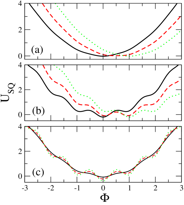
Figure 3: The rf SQUID potential $U_{SQ}$ from Eq. (10) as a function of the flux $\Phi$ threading the SQUID ring. (a) For a non-hysteretic SQUID with $\beta_{L}\simeq 0.75<1$ and $\phi_{dc}=\Phi_{dc}/\Phi_{0}=0$ (black-solid curve); $0.5$ (red-dashed curve); $1.0$ (green-dotted curve). (b) For a hysteretic SQUID with $\beta_{L}\simeq 8>1$ and $\phi_{dc}=\Phi_{dc}/\Phi_{0}=0$ (black-solid curve); $0.5$ (red-dashed curve); $1.0$ (green-dotted curve). (c) For $\Phi_{dc}=0$ and $\beta_{L}=0.5<1$ (black-solid curve); $1.5$ (red-dashed curve); $2.5$ (green-dotted curve).

Normalization.- For an appropriate normalization of the single SQUID equation (4) and the corresponding dynamic equations for the one- and two-dimensional SQUID metamaterials discussed below, the following relations are used

$$\phi=\frac{\Phi}{\Phi_{0}},~{}~{}~{}\phi_{ac}=\frac{\Phi_{ac}}{\Phi_{0}},~{}~{}~{}\phi_{dc}=\frac{\Phi_{dc}}{\Phi_{0}},~{}~{}~{}\tau=\omega_{LC}t,~{}~{}~{}\Omega=\frac{\omega}{\omega_{LC}},~{}~{}~{}i=\frac{I}{I_{c}},$$ (11)

i.e., frequency and time are normalized to $\omega_{LC}$ and its inverse $\omega_{LC}^{-1}$, respectively, while all the fluxes and currents are normalized to $\Phi_{0}$ and $I_{c}$, respectively. Then, Eq. (4) is written in normalized form as

$$\ddot{\phi}+\gamma\dot{\phi}+\beta\sin\left(2\pi\phi\right)+\phi=\phi_{ext},$$ (12)

where the overdots denote derivation with respect to the normalized temporal variable $\tau$, $\phi_{ext}=\phi_{dc}+\phi_{ac}\cos(\Omega\tau)$ is the normalized external flux, and

$$\beta=\frac{I_{c}L}{\Phi_{0}}=\frac{\beta_{L}}{2\pi},\qquad\gamma=\frac{1}{R}\sqrt{\frac{L}{C}}$$ (13)

is the rescaled SQUID parameter and dimensionless loss coefficient, respectively. The term which is proportional to $\gamma$ in Eq. (12) actually represents all of the dissipation coupled to the rf SQUID.

The properties of the many variants of the SQUID have been investigated for many years, and they can be found in a number of review articles ^{187, 188, 189, 190, 157, 160, 191}, textbooks ¹⁹², and a Handbook ^{158, 159}. Here we focus on the multistability and the tunability properties of rf SQUIDs, which are important for our later discussions on SQUID metamaterials. As it was mentioned earlier, the rf SQUID is a nonlinear oscillator which exhibits strong resonant response at a particular frequency to a sinusoidal (ac) flux field. For low amplitudes of the ac flux field, i.e., in the linear regime, the single-SQUID resonance frequency is given in Eq. (8); in units of the inductive-capacitive ($LC$) SQUID frequency, the single-SQUID resonance frequency is

$$\Omega_{SQ}=\frac{\omega_{SQ}}{\omega_{LC}}=\sqrt{1+\beta_{L}}.$$ (14)

It was theoretically demonstrated that the SQUID resonance can be tuned within a broad band of frequencies either by a dc flux bias $\phi_{dc}$ or by the amplitude of an ac flux field $\phi_{ac}$. Soon after these predictions, these tunability properties were confirmed experimentally ^{34, 134}. Further experiments showed that the single-SQUID resonance frequency is also tunable by the power of the ac flux field, as well as with temperature ¹⁶¹. In particular, with increasing the amplitude of the ac flux field from low to high values, the single-SQUID resonance frequency shifts from $\Omega=\Omega_{SQ}$ to $\Omega=1$ (i.e., towards lower frquencies). Note that for $\beta_{L}=0.86$, a typical value for $\beta_{L}$ and very close to those obtained in the experiments, the single-SQUID resonance frequency may vary from $\Omega=\Omega_{SQ}\simeq 1.364$ to $\Omega\simeq 1$, that is more than $25\%$ of variation (broad-band tunability). Moreover, the single-SQUID resonance curve, i.e., the oscillation amplitude of the flux through the SQUID loop $\phi_{max}$ as a function of the driving frequency $\Omega$, changes dramatically its shape. Such a resonance curve for relatively high ac flux amplitude $\phi_{ac}=0.06$ is shown in Fig. 4(a) ¹⁶⁶. Resonance curves like that are calculated from Eq. (12). As it can be observed, the curve ”snakes” back and forth within a narrow frequency band around the geometrical resonance frequency $\Omega\sim 1$. The solid-blue branches of the resonance curve indicate stable solutions, while the dashed-black branches indicate unstable ones (hereafter referred to as stable and unstable branches, respectively). The stable and unstable branches merge at particular points (turning points) denoted by SN; at all these points, in which $d\Omega/d\phi_{max}=0$, saddle-node bifurcations of limit cycles occur. Clearly, by looking at Fig. 4(a) one can identify that there are certain frequency bands in which more than one simultaneously stable solutions exist. For the sake of illustration, a vertical line has been drawned at $\Omega=1.007$. For that frequency, there are five (5) simultaneously stable solutions which are marked by the letters $A,B,C,D,E$, and four (4) unstable ones. This can be seen more clearly in the inset of Fig. 4(a) which shows an enlargement of the main figure around $\Omega=1.007$. Actually, at this frequency the number of possible solutions for the chosen set of simulation parameters is maximum. Thus for that set of parameters, $\Omega=1.007$ is the maximum multistability frequency. The corresponding trajectories of the stable solutions at $A-E$ are shown in the phase portraits $\dot{\phi}(\tau)-{\phi}(\tau)$ in Fig. 4(b). Multistability is enchanced (i.e., more solution branches appear) with increasing the ac flux amplitude $\phi_{ac}$ or lowering the loss coefficient $\gamma$.

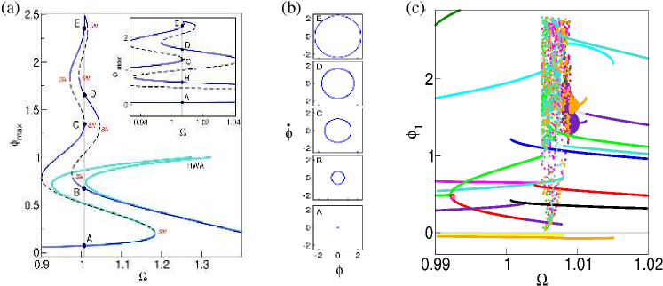
Figure 4: (a) The snake-like resonance curve for an rf SQUID with $\beta_{L}=0.86$, $\gamma=0.024$, and ac flux amplitude $\phi_{ac}=0.06$. The solid-blue and dashed-black lines correspond to branches of stable and unstable periodic solutions, respectively. Saddle-node bifurcation points are denoted as SN. The vertical thick gray line corresponds to $\Omega=1.007$, and the turquoise lines are obtained from Eq. (15). Inset: enlargement around the maximum multistability frequency $\Omega=1.007$. (b) Phase portraits for the periodic orbits at the points marked as $A-E$ on the resonance curve and in the inset. (c) A bifurcation diagram for two coupled identical SQUIDs around the single-SQUID maximum multistability frequency $\Omega=1.007$. Only stable solutions are shown for clarity. The flux though the loop of say, the first SQUID, $\phi_{1}$ is plotted at the end of the driving period (see text). The coupling coeffcient between the SQUIDs is $\lambda=-0.025$ and the other parameters as in (a). At least ten (10) stable states, including chaotic ones, are visible at $\Omega=1.007$.

An approximation to the resonance curve for $\phi_{max}\ll 1$ is given by ¹⁶⁶

$$\Omega^{2}=\Omega_{SQ}^{2}\pm\frac{\phi_{ac}}{\phi_{max}}-\beta_{L}\phi_{max}^{2}\{a_{1}-\phi_{max}^{2}[a_{2}-\phi_{max}^{2}(a_{3}-a_{4}\phi_{max}^{2})]\},$$ (15)

where $a_{1}=\pi^{2}/2$, $a_{2}=\pi^{4}/12$, $a_{3}=\pi^{6}/144$, and $a_{4}=\pi^{8}/2880$, which implicitly provides $\phi_{max}$ as a function of $\Omega$. The approximate flux amplitude - driving frequency curves from Eq. (15) are shown in Fig. 4(a) in turquoise color; clearly, they show excellent agreement with the numerical snaking resonance curve for $\phi_{max}\lesssim 0.6$. From Eq. (15), the frequency of the first saddle-node bifurcation (the one with the lowest $\phi_{max}$) can be calculated accurately. For simplicity, set $a_{2}=a_{3}=a_{4}=0$ and $a_{1}=\pi^{2}/2$ into Eq. (15) and then use the condition $d\Omega/d\phi_{max}=0$ to obtain $\phi_{max,b}=\left(\frac{\mp\phi_{ac}}{\pi^{2}\beta_{L}}\right)^{1/3}$, where $\phi_{max,b}$ is the flux amplitude at which the first saddle-node bifurcation occurs. By substitution of $\phi_{max,b}$ into the simplified Eq. (15), we get $\Omega^{2}\equiv\Omega^{2}_{b}=\Omega_{SQ}^{2}-\frac{3}{2}(\pi^{2}\beta_{L})^{1/3}\phi_{ac}^{2/3}$, where $\Omega_{b}$ is the frequency at which the first saddle-node bifurcation occurs. For the parameters used in Fig. 4(a), i.e., $\beta_{L}=0.85$ and $\phi_{ac}=0.06$, we get $\phi_{max,b}\simeq 0.192$ and $\Omega_{b}\simeq 1.18$ which agree very well with the numerics.

The dynamic complexity for frequencies around the single-SQUID resonance increases immensely in a SQUID array with a relatively large number of SQUIDS. Although the coupling between SQUIDs is discussed in detail in the next Subsection (Subsection $2.2$), we believe it is appropriate to show here the solutions around the single-SQUID multistability frequency for a system of two coupled SQUIDs (Fig. 4(c)). The two SQUIDs, $1$ and $2$, are identical, and they are coupled magnetically with strength $\lambda$ through their mutual inductances. In Fig. 4(c), the flux through the loop of SQUID $1$, $\phi_{1}$, is plotted as a function of frequency $\Omega$; since the presence of chaotic solutions was expected, the value of $\phi_{1}$ was plotted at the end of fifty (50) consecutive driving periods $T$ for each $\Omega$ (after the transients have died out). The frequency interval of Fig. 4(c) is the same as that in the inset of Fig. 4(a). Different colors have been used to help distinguishing between different solution branches; also, unstable solutions have been omitted for clarity. It can be observed that the number of stable states for the two-SQUID system is more than two times larger than the stable states of the single-SQUID. Moreover, apart from the periodic solutions, a number of (coexisting) chaotic solutions has emerged. The dynamic complexity increases with increasing the number of SQUIDs $N$ which are coupled together. This effect, which has been described in the past for certain arrays of nonlinear oscillators is named as attractor crowding ^{193, 194}. It has been argued that the number of stable limit cycles (i.e., periodic solutions) in such systems scale with the number of oscillators $N$ as $(N-1)!$. As a result, their basins of attraction crowd more and more tightly in phase space with increasing $N$. The importance of this effect for the emergence of counterintuitive collective states in SQUID metamaterials is discussed in Subsection $3.4$.

In Fig. 5, a number of flux amplitude - frequency and current amplitude-frequency curves are presented to demonstrate the tunability of the resonance frequency by varying the amplitude of the ac field $\phi_{ac}$ or by varying the dc flux bias $\phi_{dc}$. Since the properties of a SQUID-based metamaterial are primarily determined by the corresponding properties of its elements (i.e., the individual SQUIDs), the tunability of a single SQUID implies the tunability of the metamaterial itself. In Figs. 5(a) and (b) the flux amplitude - frequency curves are shown for a SQUID in the non-hysteretic and the hysteretic regime with $\beta_{L}=0.15$ and $1.27$, respectively. The ac field amplitude $\phi_{ac}$ increases from top to bottom panel. In the top panels, the SQUID is close to the linear regime and the resonance curves are almost symmetric without exhibiting visible hysteresis. A sharp resonance appears at $\Omega=\Omega_{SQ}$ as predicted from linear theory. With increasing $\phi_{ac}$ the nonlinearity becomes more and more appreciable and the resonance moves towards lower frequencies (middle and lower panels). Hysteretic effects are clearly visible in this regime. The resonance frequency of an rf SQUID can be also tuned by the application of a dc flux bias, $\phi_{dc}$, as shown in Figs. 5(c) and (d). While for $\phi_{dc}=0$ the resonance appears close to $\Omega_{SQ}$ (although slightly shifted to lower frequencies due to small nonlinear effects), it moves towards lower frequencies for increasing $\phi_{dc}$. Importantly, the variation of the resonance frequency does not seem to occur continuously but, at least for low $\phi_{dc}$, small jumps are clearly observable due to the inherently quantum nature of the SQUID which is incorporated to some extent into the phenomenological flux dynamics Eq. (12). The shift of the resonance with a dc flux bias in a single SQUID has been observed in high critical temperature (high$-T_{c}$) rf SQUIDs ¹⁹⁵, as well as in low critical temperature (low$-T_{c}$) rf SQUIDs ^{134, 161}. In Fig. 5, there was no attempt to trace all possible branches of the resonance curves for clarity, and also for keeping the current in the SQUID to values less than the critical one for the JJ, i.e., for $I<I_{c}$.

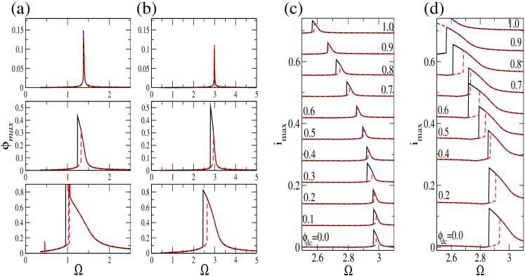
Figure 5: Flux amplitude - frequency ($\phi_{max}-\Omega$) curves for an rf SQUID with $\phi_{dc}=0$, $\gamma=0.002$, and (a) $\beta=0.15$; (b) $\beta=1.27$, and current amplitude - frequency ($i_{max}-\Omega$) curves for an rf SQUID with $\beta=1.27$, $\gamma=0.002$, and (c) $\phi_{ac}=0.01$; (d) $\phi_{ac}=0.1$. In (a) and (b), the ac field amplitude $\phi_{ac}$ increases from top to bottom panel: $\phi_{ac}=0.001$ (top); $\phi_{ac}=0.01$ (middle); $\phi_{ac}=0.1$ (bottom). In (c) and (d), the value of the dc flux bias increases from zero in steps of $0.1$ as shown.

Another illustration of the multistability in an rf SQUID is shown in Fig. 6, which also reveals an anti-resonance effect. In Figs. 6(a) and (b), the current amplitude - frequency curves are shown in two cases; one close to the weakly nonlinear regime and the other in the strongly nonlinear regime, respectively. In Fig. 6(a), the curve does not exhibit hysteresis but it is slightly skewed; the resonance frequency is $\Omega_{R}\simeq 1.25$, slightly lower than the SQUID resonance frequency in the linear regime, $\Omega_{SQ}\simeq 1.37$ (for $\beta_{L}=0.88$). In Fig. 6(b), the ac field amplitude $\phi_{ac}$ has been increased by an order of magnitude with respect to that in Fig. 6(a), and thus strongly nonlinear effects become readily apparent. Five (5) stable branches can be identified in a narrow frequency region around $\Omega\simeq 1$, i.e., around the geometrical (inductive-capacitive, $LC$) resonance frequency (unstable brances are not shown). The upper branches, which are extremely sensitive to perturbations, correspond to high values of the current amplitude $i_{max}=I_{max}/I_{c}$, which leads the JJ of the SQUID to its normal state. The red arrows in Figs. 6, point at the location of an anti-resonance ¹⁹⁶ in the current amplitude - frequency curves. Such an anti-resonance makes itself apparent as a well-defined dip in those curves, with a minimum that almost reaches zero. The effect of anti-resonance has been observed in nonlinearly coupled oscillators subjected to a periodic driving force ¹⁹⁷ as well as in parametrically driven nonlinear oscillators ¹⁹⁸. However, it has never before been observed in a single, periodically driven nonlinear oscillator such as the rf SQUID. In Figs. 6(c) and (d), enlargements of Figs. 6(a) and (b), respectively, are shown around the anti-resonance frequency. Although the ”resonance” region in the strongly nonlinear case has been shifted significantly to the left as compared with the weakly nonlinear case, the location of the anti-resonance has remained unchanged (eventhough $\phi_{ac}$ in Figs. 6(a) and (b) differ by an order of magnitude). The knowledge of the location of anti-resonance(s) as well as the resonance(s) of an oscillator or a system of oscillators, beyond their theoretical interest, it is of importance in device applications. Certainly these resonances and anti-resonances have significant implications for the SQUID metamaterials whose properties are determined by those of their elements (i.e., the individual SQUIDs). When the SQUIDs are in an anti-resonant state, in which the induced current is zero, they do not absorb energy from the applied field which can thus transpass the SQUID metamaterial almost unaffected. Thus, in such a state, the SQUID metamaterial appears to be transparent to the applied magnetic flux as has been already observed in experiments on two-dimensional SQUID metamaterials ¹⁶¹; the observed effect has been named as broadband self-induced transparency. Moreover, since the anti-resonance frequency is not affected by $\phi_{ac}$, the transparency can be observed even in the strongly nonlinear regime, for which the anti-resonance frequency lies into the multistability region. In that case, the transparency of the metamaterial may be turned on and off as it has been already discussed in Ref. ¹⁶¹. Thus, the concept of the anti-resonance serves for making a connection between an important SQUID metamaterial property and a fundamental dynamical property of nonlinear oscillators.

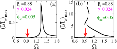
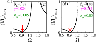
Figure 6: Current amplitude $i_{max}=I_{max}/I_{c}$ - driving frequency $\Omega$ characteristics for an rf SQUID with $\beta_{L}=0.88$, $\gamma=0.024$, $\phi_{dc}=0$, and (a) $\phi_{ac}=0.005$; (b) $\phi_{ac}=0.05$. Enlargements of (a) and (b) around the anti-resonance frequnecy are shown in (c) and (d), respectively. The red arrows point at the location of the anti-resonance.

The tunability of the SQUID resonance with a dc magnetic field and the temperature has been investigated in recent experiments ^{118, 134}. Those investigations rely on the measurement of the magnitude of the complex transmission $|S_{21}|$ as one or more external parameters such as the driving frequency, the dc flux bias, and the temperature vary. Very low values of $|S_{21}|$ indicate that the SQUID is at resonance. In Fig. 7, the resonant response is identified by the red features. In the left panel, it is observed that the resonance vary periodically with the applied dc flux, with period $\Phi_{0}$. In the middle panel of Fig. 7, the effect of the temperature $T$ is revealed; as expected, the tunability bandwidth of the resonance decreases with increasing temperature. In the right panel of Fig. 7, the variation of the resonance frequency with the applied rf power is shown. Clearly, three different regimes are observed; for substantial intervals of low and high rf power, the resonance frequency is approximatelly constant at $\Omega\sim\Omega_{SQ}$ and $\Omega\sim 1$, respectively, while for intermediate rf powers the resonance apparently dissapears. The latter effect is related to the broad-band self-induced transparency ¹⁶¹.

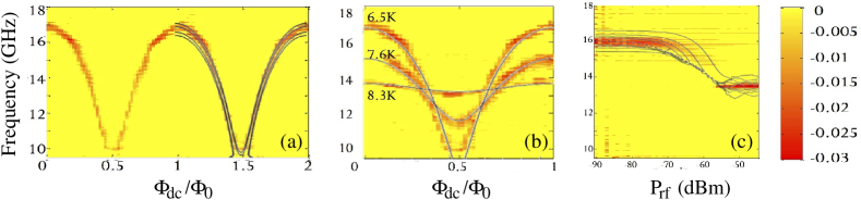
Figure 7: Experimental measurements of the complex transmission magnitude $|S_{21}|$ of an rf SQUID. The resonant response is identified by the red features. Left: $|S_{21}|$ as a function of frequency $\Omega$ and applied dc flux $\phi_{dc}$ at $-80~{}dBm$ rf power and temperature $T=6.5~{}K$. Middle: $|S_{21}|$ as a function of frequency and applied dc flux at three different temperatures, $T=6.5~{}K$, $7.6~{}K$, and $8.3~{}K$, and $-80~{}dBm$ rf power. Right: $|S_{21}|$ as a function of frequency and rf power at fixed dc flux, $\phi_{dc}=1/6$ and temperature $T=6.5~{}K$ ¹³⁴.

2.2 SQUID Metamaterials Models and Flux Wave Dispersion

Conventional (metallic) metamaterials comprise regular arrays of split-ring resonators (SRRs), which are highly conducting metallic rings with a slit. These structures can become nonlinear with the insertion of electronic devices (e.g., varactors) into their slits ^{199, 200, 80, 93, 201}. SQUID metamaterials is the superconducting analogue of those nonlinear conventional metamaterials that result from the replacement of the varactor-loaded metallic rings by rf SQUIDs as it has been suggested both in the quantum ¹³² and the classical ¹³³ regime. Recently, one- and two-dimensional SQUID metamaterials have been constructed from low critical temperature superconductors which operate close to liquid Helium temperatures ^{34, 202, 134, 161, 203, 162}. The experimental investigation of these structures has revealed several novel properties such as negative diamagnetic permeability ^{118, 34}, broad-band tunability ^{34, 134}, self-induced broad-band transparency ¹⁶¹, dynamic multistability and switching ¹³⁵, as well as coherent oscillations ¹⁶², among others. Some of these properties, i.e., the dynamic multistability effect and tunability of the resonance frequency of SQUID metamaterials, have been also revealed in numerical simulations ^{204, 164}. Moreover, nonlinear localization ¹⁶³ and the emergence of counter-intuitive dynamic states referred to as chimera states in current literature ^{165, 166, 196} have been demonstrated numerically in SQUID metamaterial models. The chimera states have been discovered numerically in rings of identical phase oscillators ¹⁶⁷ (see Ref. ¹⁶⁸ for a review).

The applied time-dependent magnetic fields induce (super)currents in the SQUID rings through Faraday’s induction law, which couple the SQUIDs together through dipole-dipole magnetic forces; although weak due to its magnetic nature, that interaction couples the SQUIDs non-locally since it falls-off as the inverse cube of their center-to-center distance. Consider a one-dimensional linear array of $N$ identical SQUIDs coupled together magnetically through dipole-dipole forces. The magnetic flux $\Phi_{n}$ threading the $n-$th SQUID loop is ¹⁶⁵

$$\Phi_{n}=\Phi_{ext}+L\,I_{n}+L\,\sum_{m\neq n}\lambda_{|m-n|}I_{m},$$ (16)

where the indices $n$ and $m$ run from $1$ to $N$, $\Phi_{ext}$ is the external flux in each SQUID, $\lambda_{|m-n|}=M_{|m-n|}/L$ is the dimensionless coupling coefficient between the SQUIDs at positions $m$ and $n$, with $M_{|m-n|}$ being their corresponding mutual inductance, and

$$-I_{n}=C\frac{d^{2}\Phi_{n}}{dt^{2}}+\frac{1}{R}\frac{d\Phi_{n}}{dt}+I_{c}\,\sin\left(2\pi\frac{\Phi_{n}}{\Phi_{0}}\right)$$ (17)

is the current in each SQUID given by the RCSJ model ⁹⁷, with $\Phi_{0}=h/(2e)$ and $I_{c}$ being the flux quantum and the critical current of the JJs, respectively. Recall that within the RCSJ framework, $R$, $C$, and $L$ are the resistance, capacitance, and self-inductance of the SQUIDs’ equivalent circuit, respectively. Combination of Eqs.(16) and (17) gives

$$C\frac{d^{2}\Phi_{n}}{dt^{2}}+\frac{1}{R}\frac{d\Phi_{n}}{dt}+\frac{1}{L}\sum_{m=1}^{N}\left({\bf\hat{\Lambda}}^{-1}\right)_{nm}\left(\Phi_{m}-\Phi_{ext}\right)+I_{c}\,\sin\left(2\pi\frac{\Phi_{n}}{\Phi_{0}}\right)=0,$$ (18)

where ${\bf\hat{\Lambda}}^{-1}$ is the inverse of the $N\times N$ coupling matrix

$$\left({\bf\hat{\Lambda}}\right)_{nm}=\left\{\begin{array}[]{ll}1,&\mbox{if $m=n$};\\ \lambda_{|m-n|}=\lambda_{1}\,|m-n|^{-3},&\mbox{if $m\neq n$},\end{array}\right.$$ (21)

with $\lambda_{1}$ being the coupling coefficient betwen nearest-neighboring SQUIDs.

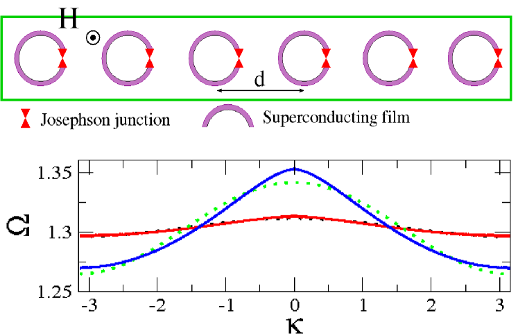
Figure 8: Upper: Schematic of a one-dimensional SQUID metamaterial. Lower: Frequency dispersion of the SQUID metamaterial with non-local coupling, for $\beta=0.1114$ ($\beta_{L}\simeq 0.7$) and $\lambda_{0}=-0.05$ (blue curve); $-0.01$ (red curve). The corresponding dispersions for nearest-neighbor (local) coupling are shown as green and black dotted curves, respectively.

The dimensionless coupling strength $\lambda_{|m-n|}=M_{|m-n|}/L$ between the SQUIDs at site $n$ and $m$ (normalized center-to-center distance $|m-n|$), can be calculated either analytically or numerically. The self-inductance $L$ of the SQUIDs, for example, can be either estimated by an empirically derived equation ²⁰⁵ or it can be calculated using commercially available software (FastHenry). The mutual inductance $M_{|m-n|}$ can also be obtained numerically from a FastHenry calculation or it can be approximated using basic expressions from electromagnetism. The magnetic field generated by a wire loop, which is the approximate geometry of a SQUID, at a distance greater than its dimensions, is given by the Biot-Savart law as $B=\frac{\mu_{0}}{4\pi}\frac{\pi r^{2}I_{w}}{d^{3}}$, where $I_{w}$ is the current in the wire, $r$ is the radius of the loop, and $d$ is the distance from the center of the loop. The mutual inductance between two such (identical) loops lying on the same plane is given by

$$M=\frac{B\pi r^{2}}{I_{w}}=\frac{\mu_{0}}{4\pi}\frac{(\pi r^{2})^{2}}{d^{3}}\propto d^{-3},$$ (22)

where it is assumed that the field $B$ is constant over the area of each loop, $\pi r^{2}$. For square loops of side $a$, the radius $r$ should be replaced by $a/\sqrt{\pi}$. Eq. (22) explains qualitatively the inverse cube distance-dependence of the coupling strength $\lambda_{|m-n|}$ between SQUIDs.

In normalized form Eq. (18) reads ($n=1,...,N$)

$$\ddot{\phi}_{n}+\gamma\dot{\phi}_{n}+\beta\sin\left(2\pi\phi_{n}\right)=\sum_{m=1}^{N}\left({\bf\hat{\Lambda}}^{-1}\right)_{nm}\left(\phi_{ext}-\phi_{m}\right),$$ (23)

where the relations given in Eq. (11) have been used. Specifically, frequency and time are normalized to $\omega_{LC}=1/\sqrt{LC}$ and its inverse $\omega_{LC}^{-1}$, respectively, the fluxes and currents are normalized to $\Phi_{0}$ and $I_{c}$, respectively, the overdots denote derivation with respect to the normalized temporal variable, $\tau$, $\phi_{ext}=\phi_{dc}+\phi_{ac}\cos(\Omega\tau)$, with $\Omega=\omega/\omega_{0}$ being the normalized driving frequency, and $\beta$, $\gamma$ are given in Eq. (13). The (magnetoinductive) coupling strength between SQUIDs, which can be estimated from the experimental parameters in Ref. ²⁰⁶, as well as from recent experiments ^{118, 34}, is rather weak due to its magnetic nature (of the order of $10^{-2}$ in normalized units). Since that strength falls-off approximatelly as the inverse-cube of the distance between SQUIDs, a model which takes into account nearest-neighbor coupling only is sufficient for making reliable predictions. In that case, the coupling matrix assumes the simpler, tridiagonal and symmetric form

$$\left({\bf\hat{\Lambda}}\right)_{nm}=\left\{\begin{array}[]{ll}1,&\mbox{if $m=n$};\\ \lambda_{1}&\mbox{if $m=n\pm 1$};\\ 0&\mbox{for any other $n$, $m$}.\end{array}\right.$$ (27)

For $\lambda_{1}\ll 1$, the inverse of the coupling matrix is approximated to order ${\cal O}(\lambda_{1}^{2})$ by

$$\left({\bf\hat{\Lambda}}^{-1}\right)_{nm}=\left\{\begin{array}[]{ll}1,&\mbox{if $m=n$};\\ -\lambda_{1}&\mbox{if $m=n\pm 1$};\\ 0&\mbox{for any other $n$, $m$}.\end{array}\right.$$ (31)

Substituting Eq. (31) into Eq. (23), the corresponding dynamic equations for the fluxes through the loops of the SQUIDs of a locally coupled SQUID metamaterial are obtained as

$$\ddot{\phi}_{n}+\gamma\dot{\phi}_{n}+\phi_{n}+\beta\sin\left(2\pi\phi_{n}\right)=\lambda(\phi_{n-1}+\phi_{n+1})+\phi_{eff},$$ (32)

where $\phi_{eff}=(1-2\lambda)\,\phi_{ext}$ is the ”effective” external flux, with $\phi_{ext}=\phi_{dc}+\phi_{ac}\cos(\Omega\tau)$ being the normalized external flux. The effective flux arises due to the nearest-neighbor approximation. For a finite SQUID metamaterial (with $N$ SQUIDs), $\phi_{eff}$ is slightly different for the SQUIDs at the end-points of the array; specifically, for those SQUIDs $\phi_{eff}=(1-\lambda)\,\phi_{ext}$ since they interact with one nearest-neighbor only.

Linearization of Eq. (23) around zero flux with $\gamma=0$ and $\phi_{ext}=0$ gives for the infinite system

$$\ddot{\phi}_{n}+\left[\beta_{L}+\left({\bf\hat{\Lambda}}^{-1}\right)_{nn}\right]\phi_{n}+\sum_{m\neq n}\left({\bf\hat{\Lambda}}^{-1}\right)_{nm}\phi_{m}=0.$$ (33)

By substitution of the plane-wave trial solution $\phi_{n}=A\,\exp[i(\kappa n-\Omega\tau)]$ into Eq. (33), with $\kappa$ being the wavevector normalized to $d^{-1}$ ($d$ is the side of the unit cell, see Fig. 1) , and using

$$\sum_{m\neq n}\left({\bf\hat{\Lambda}}^{-1}\right)_{nm}e^{i\kappa(m-n)}=2\sum_{m=1}^{\infty}\left({\bf\hat{\Lambda}}^{-1}\right)_{m}\cos(\kappa m),$$ (34)

where $m$ is the ”distance” from the main diagonal of ${\bf\hat{\Lambda}}^{-1}$, we get

$$\Omega=\sqrt{\Omega_{1}^{2}+2\sum_{m=1}^{\infty}\left({\bf\hat{\Lambda}}^{-1}\right)_{m}\cos(\kappa m)},$$ (35)

where $\Omega_{1}^{2}=\beta_{L}+\left({\bf\hat{\Lambda}}^{-1}\right)_{nn}\simeq\Omega_{SQ}^{2}$. Note that for the infinite system the diagonal elements of the inverse of the coupling matrix $\left({\bf\hat{\Lambda}}^{-1}\right)_{nn}$ have practically the same value which is slightly larger than unity. The frequency $\Omega_{1}$ is very close to the resonance frequency of individual SQUIDs, $\Omega_{SQ}$. Eq. (35) is the nonlocal frequency dispersion. By substitution of the same trial solution into Eq. (32), we get the nearest-neighbor frequency dispersion for flux waves, as

$$\Omega\equiv\Omega_{\kappa}=\sqrt{\Omega_{SQ}-2\lambda\,\cos\kappa}.$$ (36)

Eqs. (35) and (36) result in slightly different frequency dispersion curves as can be observed in the lower panel of Fig. 8 for two different values of the coupling coefficient $\lambda$.

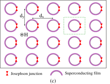
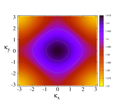
Figure 9: Left: Schematic drawing of a planar SQUID metamaterial in a time-dependent magnetic field ${\bf H}(t)$. Right: Density plot and contours of the linear frequency dispersion $\Omega_{\vec{\kappa}}$ on the $\kappa_{x}-\kappa_{y}$ plane calculated from Eq. (44), for a two-dimensional SQUID metamaterial with $\lambda_{x}=\lambda_{y}=-0.014$ and $\beta=0.15$ ($\beta_{L}=0.7$).

In order to increase the dimensionality and obtain the dynamic equations for the fluxes through the loops of the SQUIDs arranged in an orthogonal lattice, as shown in the left panel of Fig. 9 in which the unit cell is enclosed inside the green-dotted line, we first write the corresponding flux-balance relations ^{163, 207, 204},

$$\Phi_{n,m}=\Phi_{ext}+L\,\left[I_{n,m}+\lambda_{x}(I_{n-1,m}+I_{n+1,m})+\lambda_{y}(I_{n,m-1}+I_{n,m+1})\right],$$ (37)

where $\Phi_{n,m}$ is the flux threading the $(n,m)-$th SQUID of the metamaterial, $I_{n,m}$ is the total current induced in the $(n,m)-$th SQUID of the metamaterial, and $\lambda_{x,y}\equiv M_{x,y}/L$ are the magnetic coupling coefficients between neighboring SQUIDs, with $M_{x}$ and $M_{y}$ being the mutual inductances in the $x$ and $y$ directions, ($M_{x},M_{y}<0$). The subscripts $n$ and $m$ run from $1$ to $N_{x}$ and $1$ to $N_{y}$, respectively. The current $I_{n,m}$ is given by the RCSJ model as

$$-I_{n,m}=C\frac{d^{2}\Phi_{n,m}}{dt^{2}}+\frac{1}{R}\frac{d\Phi_{n,m}}{dt}+I_{c}\,\sin\left(2\pi\frac{\Phi_{n,m}}{\Phi_{0}}\right).$$ (38)

Eq. (37) can be inverted to provide the currents as a function of the fluxes, and then it can be combined with Eq. (38) to give the dynamic equations ¹⁶³

$$C\frac{d^{2}\Phi_{n,m}}{dt^{2}}+\frac{1}{R}\frac{d\Phi_{n,m}}{dt}+\Phi_{n,m}+I_{c}\,\sin\left(2\pi\frac{\Phi_{n,m}}{\Phi_{0}}\right)-\lambda_{x}(\Phi_{n-1,m}+\Phi_{n+1,m})-\lambda_{y}(\Phi_{n,m-1}+\Phi_{n,m+1})$$

$$=[1-2(\lambda_{x}+\lambda_{y})]\Phi_{ext}.$$ (39)

In the absence of losses ($\gamma=0$), the earlier equations can be obtained from the Hamiltonian function

$$H=\sum_{n,m}\frac{Q_{n,m}^{2}}{2C}+\sum_{n,m}\left[\frac{1}{2L}(\Phi_{n,m}-\Phi_{ext})^{2}-E_{J}\,\cos\left(2\pi\frac{\Phi_{n,m}}{\Phi_{0}}\right)\right]-\sum_{n,m}\frac{\lambda_{x}}{L}(\Phi_{n,m}-\Phi_{ext})(\Phi_{n-1,m}-\Phi_{ext})$$

$$-\sum_{n,m}\frac{\lambda_{y}}{L}(\Phi_{n,m}-\Phi_{ext})(\Phi_{n,m-1}-\Phi_{ext}),$$ (40)

where

$$Q_{n,m}=C\,\frac{d\Phi_{n,m}}{dt}$$ (41)

is the canonical variable conjugate to $\Phi_{n,m}$, and represents the charge accumulating across the capacitance of the JJ of each rf SQUID. The above Hamiltonian function is the weak coupling version of that proposed in the context of quantum computation ²⁰⁸. Eqs. (2.2) can be written in normalized form as

$$\ddot{\phi}_{n,m}+\gamma\dot{\phi}_{n,m}+\phi_{n,m}+\beta\,\sin(2\pi\phi_{n,m})-\lambda_{x}(\phi_{n-1,m}+\phi_{n+1,m})-\lambda_{y}(\phi_{n,m-1}+\phi_{n,m+1})=\phi_{eff},$$ (42)

where the overdots denote differentiation with respect to the normalized time $\tau$, and

$$\phi_{eff}=[1-2(\lambda_{x}+\lambda_{y})]\phi_{ext};\qquad\phi_{ext}=\phi_{dc}+\phi_{ac}\cos(\Omega\tau).$$ (43)

The frequency dispersion of linear flux-waves in two-dimensional SQUID metamaterials can be obtained with the standard procedure, by using plane wave trial solutions into the linearized dynamic equations (42). That procudure results in the relation

$$\Omega\equiv\Omega_{\bf\kappa}=\sqrt{\Omega_{SQ}^{2}-2(\lambda_{x}\,\cos\kappa_{x}+\lambda_{y}\,\cos\kappa_{y})},$$ (44)

where ${\bf\kappa}=(\kappa_{x},\kappa_{y})$ is the normalized wavevector. The components of ${\bf\kappa}$ are related to those of the wavevector in physical units ${\bf k}=(k_{x},k_{y})$ through $\kappa_{x,y}=d_{x,y}\,k_{x,y}$ with $d_{x}$ and $d_{y}$ being the wavevector component and center-to-center distance between neighboring SQUIDs in $x-$ and $y-$direction, respectively. A density plot of the frequency dispersion equations (44) on the $\kappa_{x}-\kappa_{y}$ plane is shown in the right panel of Fig. 8 for a tetragonal (i.e., $d_{x}=d_{y}$) SQUID metamaterial. Assuming thus that the coupling is isotropic, i.e., $\lambda_{x}=\lambda_{y}=\lambda$, the maximum and minimum values of the linear frequency band are then obtained by substituting ${\bf\kappa}=(\kappa_{x},\kappa_{y})=(0,0)$ and $(\pi,\pi)$, respectively, into Eq. (44). Thus we get

$$\omega_{max}=\sqrt{1+\beta_{L}+4|\lambda|},\qquad\omega_{min}=\sqrt{1+\beta_{L}-4|\lambda|},$$ (45)

that give an approximate bandwidth $\Delta\Omega\simeq 4|\lambda|/\Omega_{SQ}$.

Note that the dissipation term $+\frac{1}{R}\frac{d\Phi_{n,m}}{dt}$ appearing in Eq. (2.2) may result from the corresponding Hamilton’s equations with a time-dependent Hamiltonian ¹⁶³

$$H=e^{-t/\tau_{C}}\,\sum_{n,m}\frac{Q_{nm}^{2}}{2C}+e^{+t/\tau_{C}}\,\sum_{n,m}\left[\frac{1}{2L}(\Phi_{nm}-\Phi_{ext})^{2}-E_{J}\,\cos\left(2\pi\frac{\Phi_{nm}}{\Phi_{0}}\right)\right]$$

$$-\sum_{n,m}\left[\frac{\lambda_{x}}{L}(\Phi_{nm}-\Phi_{ext})(\Phi_{n-1,m}-\Phi_{ext})+\frac{\lambda_{y}}{L}(\Phi_{nm}-\Phi_{ext})(\Phi_{n,m-1}-\Phi_{ext})\right],$$ (46)

where $E_{J}\equiv\frac{I_{c}\,\Phi_{0}}{2\pi}$ is the Josephson energy, $\tau_{C}=R\,C$, and

$$Q_{nm}=e^{+t/\tau_{C}}\,C\,\frac{d\Phi_{nm}}{dt}$$ (47)

is the new canonical variable conjugate to $\Phi_{nm}$ which represents the generalized charge across the capacitance of the JJ of each rf SQUID. The Hamiltonian in Eq. (2.2) is a generalization in the two-dimensional lossy case of that employed in the context of quantum computation with rf SQUID qubits ^{208, 209}.

2.3 Wide-Band SQUID Metamaterial Tunability with dc Flux

An rf SQUID metamaterial is shown to have qualitatively the same behavior as a single rf SQUID with regard to dc flux and temperature tuning. Thus, in close similarity with conventional, metallic metamaterials, rf SQUID metamaterials acquire their electromagnetic properties from the resonant characteristics of their constitutive elements, i.e., the individual rf SQUIDs. However, there are also properties of SQUID metamaterials that go beyong those of individual rf SQUIDs; these emerge through collective interaction of a large number of SQUIDs forming a metamaterial. Numerical simulations using the SQUID metamaterial models presented in the previous sub-section confirm the experimentally observed tunability patterns with applied dc flux in both one and two dimensions. Here, numerical results for the two-dimensional model are presented; however, the dc flux tunability patterns for either one- or two-dimensional SQUID metamaterials are very similar. Due to the weak coupling between SQUIDs, for which the coupling coefficient has been estimated to be of the order of $10^{-2}$ in normalized units ¹⁶¹, the nearest-neighbor coupling between SQUIDs provides reliable results. The normalized equations for the two-dimensional model equations (42) are ^{163, 204}

$$\ddot{\phi}_{n,m}+\gamma\dot{\phi}_{n,m}hi_{n,m}+\beta\,\sin(2\pi\phi_{n,m})-\lambda_{x}(\phi_{n-1,m}+\phi_{n+1,m})-\lambda_{y}(\phi_{n,m-1}+\phi_{n,m+1})=\phi_{eff},$$ (48)

where $\phi_{eff}=[1-2(\lambda_{x}+\lambda_{y})]\phi_{ext}$ and $\phi_{ext}=\phi_{dc}+\phi_{ac}\cos(\Omega\tau)$. The total (symmetrized) energy of the SQUID metamaterial, in units of the Josephson energy $E_{J}$, is then

$$E_{tot}=\sum_{n,m}\left\{\frac{\pi}{\beta}\left[\dot{\phi}_{n,m}^{2}+(\phi_{n,m}-\phi_{ext})^{2}\right]+1-\cos(2\pi\phi_{n,m})\right\}$$

$$-\frac{\pi}{\beta}\sum_{n,m}\left\{\left[\lambda_{x}(\phi_{n,m}-\phi_{ext})(\phi_{n-1,m}-\phi_{ext})+\lambda_{x}(\phi_{n+1,m}-\phi_{ext})(\phi_{n,m}-\phi_{ext})\right.\right.$$

$$\left.\left.+\lambda_{y}(\phi_{n,m-1}-\phi_{ext})(\phi_{n,m}-\phi_{ext})+\lambda_{y}(\phi_{n,m}-\phi_{ext})(\phi_{n,m+1}-\phi_{ext})\right]\right\}.$$ (49)

For $\phi_{ext}=\phi_{dc}$, the average of that energy over one period $T$ of evolution

$$<E_{tot}>_{T}=\frac{1}{T}\int_{0}^{T}d\tau E_{tot}(\tau),$$ (50)

where $T=2\pi/\Omega$ with $\Omega$ being the normalized driving frequency, is constant when the obtained solution is locked to that driving frequency. In the following, the term ”tunability of the resonance” for the SQUID metamaterial is used; however, the notion of the resonance is rather appropriate for a single SQUID only. The SQUID metamaterial is capable of absorbing substantial amount of energy for frequencies within its linear frequency band, given by Eq. (44); however, the energy absorption in that band is far from being uniform. Thus, the term ”tunability of the resonance” for the SQUID metamaterial refers to that frequency at which the highest absorption of energy occurs (also note that for strong nonlinearities, the SQUID metamaterial can absorb significant amount of energies in other frequency bands as well, see next Section). Typical resonance tunability patterns are shown in Fig. 10 as density plots of $<E_{tot}>_{\tau}$ as a function of the driving frequency $f$ (in nutural units) and the dc flux bias $\phi_{dc}$ for several combinations of $\phi_{ac}$ and $\lambda_{x}=\lambda_{y}$. Note that the energy background in Fig. 10 has been removed for clarity. The thick lines with darker color depict the regions of the map with high energy absorption. The parameters used in the calculations are similar to the experimental ones ^{34, 134, 161}, although no attempt was made to exactly fit the observed patterns. These parameter values are consistent with a single-SQUID resonance frequency $f\simeq 15~{}GHz$, which is also used in the calculations and to express the frequency in natural units. In Fig. 10, the ac flux amplitude $\phi_{ac}$ increases from left to right, while the coupling $\lambda_{x}=\lambda_{y}$ increases from top bottom. The resonance become stronger as we move from the left to the right panels, as the nonlinear effects become more and more important with increasing $\phi_{ac}$. When going from top to bottom panels, with increasing $|\lambda_{x}|=|\lambda_{y}|$, a smearing of the resonance is observed, along with the appearence of secondary resonances. The latter manifest themselves as thin red (dark) curves that are located close to the main shifting pattern, and they are better seen around half-intefger values of the applied dc flux. In order to obtain accurate tunability patterns, a few hundreds of absorbed energy-frequency curves (one for each $\phi_{dc}$) have been calculated. Eqs. (48) are typically integrated with a fourth-order Runge-Kutta algorithm with constant time-step.

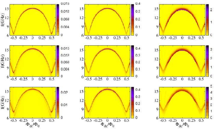
Figure 10: Density plot of the total energy per SQUID, $E_{tot}$, averaged over a period $T$ of temporal evolution, as a function of the dc flux bias $\phi_{dc}=\Phi_{dc}/\Phi_{0}$ and the driving frequency $f$, for $N_{x}=N_{y}=11$, $\beta_{L}\simeq 0.7$, $\gamma=0.009$, and several combinations of ac flux amplitude $\phi_{ac}$ and coupling coefficients $\lambda_{x}=\lambda_{y}$ (tetragonal lattice). The ac flux amplitude $\phi_{ac}$ increases from left to right, while the coupling increases from top bottom. First row: $\lambda_{x}=\lambda_{y}=-0.01$, and $\phi_{ac}=1/5000$ (left); $1/1000$ (middle); $1/200$ (right). Second row: $\lambda_{x}=\lambda_{y}=-0.03$, and $\phi_{ac}=1/5000$ (left); $1/1000$ (middle); $1/200$ (right). Third row: $\lambda_{x}=\lambda_{y}=-0.05$, and $\phi_{ac}=1/5000$ (left); $1/1000$ (middle); $1/200$ (right). The single-SQUID resonance frequency $f_{SQ}$ used in the calculations is set to $15~{}GHz$.

Experimentally, the resonance tunability patterns are obtained by measuring the magnitude of the microwave complex transmission $|S_{21}|$ (in $dB$s) of the SQUID metamaterials ^{34, 134}. The samples, which are either quasi-one-dimensional or two-dimensional, comprise nominally identical elements and they were placed inside coplanar waveguides. When excited by a weak microwave (rf) signal in the presence of a dc flux bias, the resonances of the SQUID metamaterials can be detected as dips in the frequency-dependent $|S_{21}|(\omega)$ through the waveguide. The resulting wide-band tunability patterns, shown in Fig. 11(a) and (b) for quasi-one-dimensional and two-dimensional SQUID metamaterials, respectively, clearly exhibit a periodicity in the dc flux of $\Phi_{0}$. Note the similarity between these patterns and those obtained for a single SQUID in Fig. 7. Since the coupling between SQUIDs is weak, their frequency bands are very narrow; however, the red (dark) regions indicating resonant response are actually thinner that the corresponding frequency bandwidths. This is because the resonant response is very strong at some particular frequencies, seemingly close to the maximum frequency of the band. The frequency of highest and lowest response is obtained for dc flux equal to integer and half-integer multiples of the flux quantum $\Phi_{0}$, respectively, as it can be seen clearly in Fig. 11(b) which actually contains two patterns for different temperatures, i.e., for $T\simeq 6.5~{}K$ and $T\simeq 7.9~{}K$. The resonance frequency for the lowest temperature pattern varies with the dc flux from approximately $15~{}GHz$ to $21.5~{}GHz$, providing nearly $30\%$ tunability! The tunability range reduces with increasing temperature, as can be readily inferred by comparing the data for the two different temperatures. With an increase of temperature from $T\simeq 6.5~{}K$ to $T\simeq 7.9~{}K$, the tunability range has been almost halved. Note that similar behavior is observed in the corresponding curves for a single SQUID. The resonant response of the SQUID metamaterial is stronger close to dc fluxes equal to integer multiples of $\Phi_{0}$ (this is visible in both subfigures of Fig. 11). Thus, a ”useful” frequency range can be identified in which the depth of the resonance does not change considerably with $\phi_{dc}$. In Fig. 11(a), that range lies between $13~{}GHz$ and $14.5~{}GHz$ ³⁴.

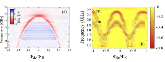
Figure 11: Measured magnitude of the complex transmission $|S_{21}|$ as a function of the driving frequency $f$ of a weak ac flux field and the applied dc flux bias $\phi_{dc}=\Phi_{dc}/\Phi_{0}$ for (a) a quasi-one-dimensional rf SQUID metamaterials (in a double-chain configuration with each chain comprising $54$ rf SQUIDs) ³⁴; (b) a two-dimensional ($27\times 27$) rf SQUID metamaterial ¹³⁴. In both figures the red (dark) features indicate regions of reduced transmission, which corresponds to resonant response. The solid-grey lines in (b) are the calculated single-SQUID resonance frequencies.

Another interesting effect which is clearly visible in the fist column of Fig. 10, corresponding to low $\phi_{ac}$ (closer to the linear limit), is the slight increase of the resonance frequency at $\phi_{dc}=0$ of the SQUID metamaterial with increasing the magnitude of the coupling coefficients $\lambda_{x}=\lambda_{y}$. This effect, as well as the shape of the resonant response for $\phi_{dc}$ between $-1/2$ and $+1/2$ can be understood within an approximate treatment which is valid for low ac field amplitudes $\phi_{ac}$. Assume that $\phi_{n,m}\simeq\phi$ for any $n,m$, i.e., that the SQUIDs are synchronized ²⁰⁴ (note that small deviations from complete synchronization always appear for finite size SQUID metamaterials). Then substitute $\phi_{n,m}=\phi$, and $\gamma=0$, $\lambda_{x}=\lambda_{y}=\lambda$ into Eqs. (48) to get

$$\ddot{\phi}+(1-4\lambda)\phi+\beta\,\sin(2\pi\phi)=(1-4\lambda)(\phi_{dc}+\phi_{ac}\cos(\Omega t).$$ (51)

In the earlier equation we further use the approximation $\beta\sin(2\pi\phi)\simeq\beta_{L}\phi-\frac{2\pi^{2}}{3}\beta_{L}\phi^{3}$, and the ansatz $\phi=\phi_{0}+\phi_{1}\cos(\Omega t)$. Substituting into Eq. (51), using the rotating wave approximation (RWA), and separating constant from time-dependent terms, we get

$$\frac{2\pi^{2}}{3}\beta_{L}\phi_{0}^{3}-(1-4\lambda+\beta_{L})\phi_{0}-\frac{3}{2}\phi_{0}\phi_{1}^{2}+(1-4\lambda)\phi_{dc}=0,\qquad\frac{\pi^{2}}{2}\beta_{L}\phi_{1}^{3}-\left\{(1-4\lambda+\beta_{L}-\Omega^{2})-2\pi^{2}\beta_{L}\phi_{0}^{2}\right\}\phi_{1}+(1-4\lambda)\phi_{ac}=0.$$ (52)

Limiting ourselves to the case $\phi_{1}<\phi_{0}<<1$, we may simplify Eqs. (52) by neglecting terms proportional to $\phi_{1}^{3}$, $\phi_{0}^{3}$, and $\phi_{0}\phi_{1}^{1}$. Note that we keep the term $\propto\phi_{0}^{2}\phi_{1}$, i.e., the lowest order coupling term between the two equations. Then, the resulting equations can be easily solved to give

$$\phi_{0}=\frac{(1-4\lambda)\phi_{dc}}{(1-4\lambda+\beta_{L})};\qquad\phi_{1}=\frac{(1-4\lambda)\phi_{ac}}{\left\{(1-4\lambda+\beta_{L}-\Omega^{2})-2\pi^{2}\beta_{L}\phi_{0}^{2}\right\}}.$$ (53)

Obviously, the ac flux amplitude in the SQUIDs, $\phi_{1}$, attains its maximum value when the expression in the curly brackets in the denominator of Eq. (53) is zero. Solving that expression for $\Omega$, we get

$$\Omega=\sqrt{(1-4\lambda+\beta_{L})-(2\pi^{2}\beta_{L})\frac{(1-4\lambda)^{2}\phi_{dc}^{2}}{(1-4\lambda+\beta_{L})^{2}}},$$ (54)

or, in natural units

$$f=\frac{f_{SQ}}{\sqrt{1+\beta_{L}}}\sqrt{(1-4\lambda+\beta_{L})-(2\pi^{2}\beta_{L})\frac{(1-4\lambda)^{2}\phi_{dc}^{2}}{(1-4\lambda+\beta_{L})^{2}}},$$ (55)

which corresponds to the ”resonance frequency” of the SQUID metamaterial itself, with $f_{SQ}$ being the single-SQUID resonance frequency. This is exactly the frequency for which the resonant response of the SQUID metamaterial is stronger. Moreover, the dependence of that frequency on the coupling coefficients, which has been experimentally observed and also seen in the numerical simulations, implies that at that frequency the SQUIDs in the metamaterials exhibit a high degree of synchronization.

From the actual numerical data of the resonance tunability patterns presented in the left column of Fig. 10 (low $\phi_{ac}$), which are calculated for increasing magnitude of the coulping coefficients (from top to bottom), the maximum response frequency has been extracted by simply identifying that frequency at which $<E_{tot}>_{\tau_{i}}$ is maximum. These curves, for $\lambda_{x}=\lambda_{y}=\lambda=-0.01$, $-0.03$, and $-0.05$, are shown in Fig. 12a, b, and c, respectively, along with the corresponding ones calculated from Eq. (55). The simple expression (55), which contains only two parameters, $\lambda$ and $\beta_{L}$, fairly agrees with the simulations for $\phi_{ac}\ll 1$ in a rather wide region of dc fluxes, i.e., from $\phi_{dc}\sim-0.3$ to $\sim+0.3$. Within this interval, the resonance frequency in Fig. 12a may change from $\Omega=1.12$ to $1.32$ that makes a variation of $\sim 15\%$. Similar tunability ranges are observed in Figs. 12b and c. For larger $\phi_{dc}$, the importance of the term $\propto\phi_{0}^{3}$ increases and it cannot be neglected for the solutions of Eqs. (52). However, the agreement between the two curves seems to get better for larger $|\lambda|$. By setting $\phi_{dc}=0$ in Eq. (55) we get that $f=\frac{f_{SQ}}{\Omega_{SQ}}\sqrt{(\Omega_{SQ}^{2}-4\lambda)}$, which, for $f_{SQ}=15~{}GHz$, $\Omega_{SQ}=1.304$ ($\beta_{L}=0.7$), $\lambda=-0.01,~{}-0.03,~{}-0.05$ gives respectively, $f=15.2,~{}15.5,15.9~{}GHz$ in agreement with the numerical results (Fig. 12). The $\lambda-$dependence of the SQUID metamaterial resonance frequency is weaker in the corresponding one-dimensional case.

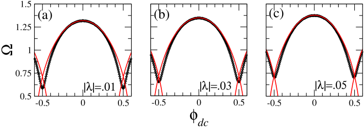
Figure 12: Normalized frequency at maximum response of the SQUID metamaterial, $\Omega$, as a function of the applied dc flux, $\phi_{dc}$, in the presence of a low-amplitude ac flux $\phi_{ac}$. The black circles have been extracted from the numerical data of Fig. 10, while the red solid lines are plotted from Eq. (54). Parameters: $N_{x}=N_{y}=11$, $\phi_{ac}=1/5000$, $\gamma=0.009$, $\beta_{L}=0.7$, and (a) $\lambda_{x}=\lambda_{y}=-0.01$; (b) $\lambda_{x}=\lambda_{y}=-0.03$; (c) $\lambda_{x}=\lambda_{y}=-0.05$.

The resonance shift due to nonlinearity has been actually observed in a Josephson parametric amplifier driven by fields of different power levels ²¹⁰, while the shift with applied dc flux has been observed in high$-T_{c}$ rf SQUIDs ¹⁹⁵ and very recently in a low$-T_{c}$ rf SQUID in the linear regime ¹¹⁸. Systematic measurements on microwave resonators comprising SQUID arrays are presented in Refs. ^{210, 211}.

2.4 Energy Transmission in SQUID Metamaterials

Conventional SRR-based metamaterials, are capable of transmitting energy through the array of resonators (i.e., the SRRs), carried by a new kind of waves, the so-called magnetoinductive waves ^{33, 212, 213, 47, 51, 214}, which have been actually observed in one-dimensional SRR arrays with a relatively small number of elements ^{48, 50}. Very much in the same way, SQUID metamaterials are capable of transmitting energy through magnetoinductive flux waves. In order to investigate the transmission of energy through a SQUID metamaterial, a one-dimensional array of SQUIDs comprising $N=54$ identical elements with $\beta_{L}=0.7$ ($\beta=0.1114$) locally coupled to their nearest neighbors, is considered. That array is driven at one end (say the left end, that with $n=1$) by an ac flux field of amplitude $\phi_{ac}$ and frequency $\Omega$. Then, Eqs. (32) become

$$\ddot{\phi}_{n}+\gamma\dot{\phi}_{n}+\phi_{n}+\beta\,\sin(2\pi\phi_{n})-\lambda(\phi_{n-1}+\phi_{n+1})=(1-2\lambda)\phi_{ext}\,\delta_{n,1},$$ (56)

where the Kroneckers’ delta $\delta_{n,1}$ indicates that only the SQUID with $n=1$ is driven by the ac field $\phi_{ext}=\phi_{ac}\,\cos(\Omega\tau)$. The total energy in this case is obtained by appropriate modification of Eq. (2.3), as

$$E_{tot}=\sum_{n=1}^{N}\left\{\frac{\pi}{\beta}\left[\dot{\phi}_{n}^{2}+(\phi_{n}-\phi_{ext}\delta_{n,1})^{2}\right]+\left[1-\cos(2\pi\phi_{n})\right]\right\}$$

$$-\frac{\pi}{\beta}\sum_{n=1}^{N}\left[\lambda(\phi_{n}-\phi_{ext}\delta_{n,1})(\phi_{n-1}-\phi_{ext}\delta_{n,1})+\lambda(\phi_{n+1}-\phi_{ext}\delta_{n,1})(\phi_{n}-\phi_{ext}\delta_{n,1})\right].$$ (57)

The dynamic equations (56) implemented with the boundary conditions $\phi_{0}=\phi_{N+1}=0$ are integrated in time until transients are eliminated and the system reaches a stationary state. Typically, $12000\,T$ time units of time-integration, where $T=2\pi/\Omega$, are sufficient for that purpose. The energy density of the SQUID metamaterial is calculated as a function of time from Eq. (2.4) for $\tau_{i}=2000\,T$ time units more; then, the decimal logarithm of the energy density averaged over $\tau_{i}$, $\log_{10}[<E_{n}>_{\tau_{i}}]$, is mapped on the frequency $\Omega$ - site number $n$ plane and shown in Fig. 13 (high transmission regions are indicated with darker colors). In Fig. 13, the quantity $\log_{10}[<E_{n}>_{\tau_{i}}]$ is shown for three different values of the dissipation coefficient $\gamma$ for fixed $\lambda=-0.01$ and $\phi{ac}=0.1$. For that value of $\phi{ac}$, the nonlinear effects become stronger for lower $\gamma$. The $\log_{10}[<E_{n}>_{\tau_{i}}]$ map for relatively strong dissipation ($\gamma=0.009$) is shown in the upper panel of Fig. 13; apparently, significant energy transmission occurs in a narrow band, of the order of $\sim 2\lambda$ around the single SQUID resonance frequency $\Omega_{SQ}\simeq 1.3$ (for $\beta_{L}=0.7$). This band almost coincides with the linear band for the one-dimensional SQUID metamaterial. Note that energy transmission also occurs at other frequencies; e.g., at $\Omega\sim 0.43$ that corresponds to a subharmonic resonance ($1/3$). Subharmonic resonances result from nonlinearity; in this case, nonlinear effects are already significant due to the relatively high $\phi_{ac}$ for all values of $\gamma$. However, for decreasing $\gamma$ (middle panel), more energy is transmitted both at frequencies in the linear band and the subharmonic resonance band. In the following we refer to the latter as the nonlinear band, since it results from purely nonlinear effects. With further decrease of $\gamma$ (lower panel), the transmitted energy in these two bands becomes more significant. The comparison can be made more clear by looking at the panels in the middle and right columns of Fig. 13, which show enlarged regions of the corresponding panels in the left column. The enlargement around the linear band (middle column) clearly reveals the increase of the transmitted energy with decreasing $\gamma$. For frequencies in the subharmonic nonlinear band, the SQUID metamaterial becomes transparent; that type of self-induced transparency due to nonlinearity is a robust effect as can be seen in Fig. 13 (right column panels), in which the loss coefficient has been varied by almost an order of magnitude. Moreover, in the case of very low losses ($\gamma=0.001$) the linear band splits into two bands, in which significant energy transmission occurs. Of those bands, the one at lower frequencies is also a nonlinear band; that phenomenon of energy transmission in the gap of the linear band(s) is known as supratransmission ²¹⁵. In the density plots of Fig. 13, the upper boundary is a reflecting one, which allows for the formation of stationary flux wave states in the SQUID metamaterial. However, similar calculations performed with a totally absorbing boundary give practically identical results.

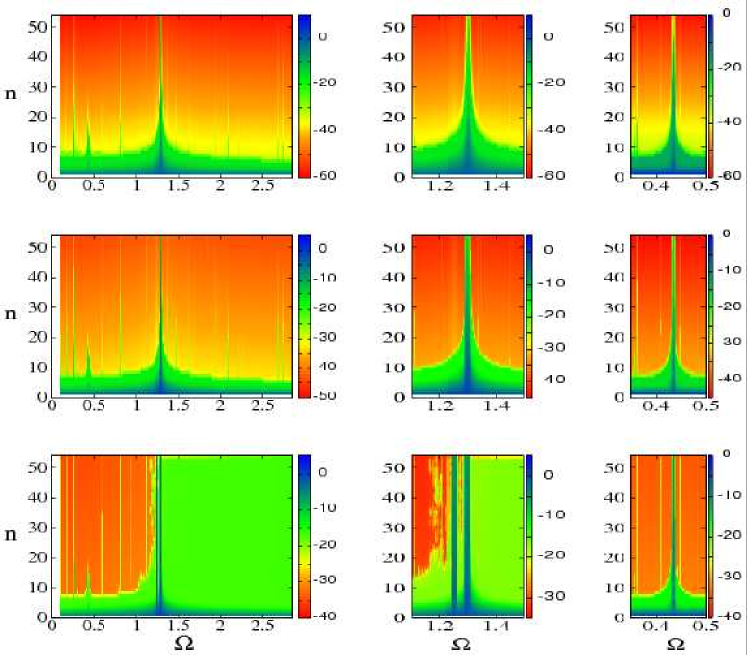
Figure 13: Energy transmission through a one-dimensional SQUID metamaterial with $N=54$ SQUIDs. The decimal logarithm of the energy density averaged over $\tau_{i}=2000\,T$ time units, $\log_{10}[<E_{n}>_{\tau_{i}}]$, is mapped on the frequency $\Omega$ - site-number $n$ plane for $\beta_{L}=0.7$ ($\beta=0.1114$), $\lambda=-0.01$, $\phi{ac}=0.1$, and $\gamma=0.009$ (upper); $\gamma=0.004$ (middle); $\gamma=0.001$ (lower). The middle and left columns are enlargements of frequency bands around the fundamental and the subharmonic resonance, respectively, at $\Omega\simeq 1.302$ and $0.43$.

In ac driven SQUID metamaterials, the significance of nonlinear effects depends both on $\gamma$ and $\phi_{ac}$. For fixed, low $\gamma$ and $\phi_{ac}\ll 1$, the dynamics is essentially close to be linear, and consequntly the energy transmission through a SQUID metamaterial is limited to frequencies within the linear band. The strength of nonlinear effects increases, however, with increasing $\phi_{ac}$, resulting in the opening of nonlinear energy transmission bands just as in the case in which $\gamma$ is varied. In Fig. 14, maps of $\log_{10}[<E_{n}>_{\tau_{i}}]$ are shown for a SQUID metamaterial with $\beta_{L}=8$ (note that with that choice of $\beta_{L}$ the SQUIDs are hysteretic). For each of the Figs. 14a-d, enlargements of the frequency bands around the $L\,C$ frequency ($\Omega=1$) and $\Omega_{SQ}$ are shown in the panels of the middle and right columns, respectively. For low ac field amplitude $\phi_{ac}$ (Fig. 14a), a significant amount of energy is transmitted through around $\Omega_{SQ}=3$, as indicated by the orange vertical line that is clearly visible in the left panel which corresponds to the linear band. With increasing $\phi_{ac}$, nonlinearity starts becoming important, and the indications of nonlinear transmission are clearly visible in Fig. 14b. Although on a large scale it appears as a widening of the linear band, a closer look (right panel) shows that there are actually two distinct bands; the linear band, and a second band which emerges at frequencies below it. Both the linear and the nonlinear bands have approximately the same width. In the middle panel, a faint orange vertical line indicates that a small amount of energy is also transmitted through the array at the $L\,C$ frequency. With further increasing $\phi_{ac}$ (Fig. 14c), the distance separating the nonlinear from the linear band increases; specifically, while the linear band remains at frequencies around $\Omega_{SQ}$, the nonlinear band shifts to lower frequencies due to nonlinearity. In this case, the energy transmitted at the $L\,C$ frequency also becomes significant (middle panel). In Fig. 14d, the ac field amplitude has been increased to $\phi_{ac}=0.2$, where the nonlinearity dominates. While the two main bands still persist (with the nonlinear band being shifted to even lower frequencies), more, narrower bands seem to appear, while the energy transmission at $\Omega\simeq 1$ becomes even more significant.

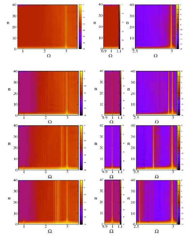
Figure 14: Energy transmission through a one-dimensional SQUID metamaterial with $N=40$ SQUIDs. The decimal logarithm of the energy density averaged over $\tau_{i}=2000\,T$ time units, $\log_{10}[<E_{n}>_{\tau_{i}}]$, is mapped on the frequency $\Omega$ - site-number $n$ plane for $\beta=1.27$ ($\beta_{L}\simeq 8$), $\gamma=0.001$, $\lambda=-0.014$, and (a) $\phi_{ac}=0.001$; (b) $\phi_{ac}=0.01$; (c) $\phi_{ac}=0.1$; (d) $\phi_{ac}=0.2$. From (a) to (d), the panels in the middle and right columns are enlarged regions of the panels in the left column; middle panels enlarge the frequency region around the $L\,C$ resonance, while the right panels enlarge the frequency region around the single SQUID resonance $\Omega_{SQ}$. Red-orange regions indicate the frequency bands in which energy transmission is high.

For very low $\phi_{ac}$ ($\phi_{dc}=0$), Eqs. (56) can be linearized to

$$\ddot{\phi}_{n}+\gamma\dot{\phi}_{n}+\Omega_{SQ}^{2}\phi_{n}-\lambda(\phi_{n-1}+\phi_{n+1})=\bar{\phi}_{ac}\cos(\Omega\tau)\,\delta_{n,1},$$ (58)

where $\bar{\phi}_{ac}=(1-2\lambda)\phi_{ac}$. If we further neglect the loss term, Eqs. (58) can be solved exactly in closed form for any $\Omega$ and for any finite even $N$, where $N$ is the total number of SQUIDs in the one-dimensional metamaterial. By substitution of the trial solution $\phi_{n}=q_{n}\cos(\Omega\tau)$ into Eqs. (58) and after some rearrangement we get

$$sq_{n-1}+q_{n}+sq_{n+1}=\kappa_{0}\,\delta_{n,1},$$ (59)

where

$$s=-\frac{\lambda}{\Omega_{SQ}^{2}-\Omega^{2}},\qquad\kappa_{0}=\frac{\bar{\phi}_{ac}}{\Omega_{SQ}^{2}-\Omega^{2}},$$ (60)

or, in matrix form

$${\bf q}=\kappa_{0}\,\hat{\bf S}^{-1}{\bf E}_{1},$$ (61)

where ${\bf q}$ and ${\bf E}_{1}$ are $N-$dimensional vectors with componets $q_{n}$ and $\delta_{n,1}$, respectively, and $\hat{\bf S}^{-1}$ is the inverse of the $N\times N$ coupling matrix $\hat{\bf S}$. The latter is a real, symmetric, tridiagonal matrix that has its diagonal elements equal to unity, while all the other non-zero elements are equal to $s$. The elements of the matrix $\hat{\bf S}^{-1}$ can be obtained in closed analytical form ²¹⁶ using known results for the inversion of more general tridiagonal matrices ²¹⁷. Then, the components of the ${\bf q}$ vector can be written as

$$q_{n}=\kappa_{0}\left(\hat{\bf S}^{-1}\right)_{n,1},$$ (62)

where $\left(\hat{\bf S}^{-1}\right)_{n,1}$ is the $(n,1)-$element of $\hat{\bf S}^{-1}$, whose explicit form is given in reference ²¹⁶. Then, the solution of the linear system of Eqs. (59) with $\gamma=0$ is

$$\phi_{n}(\tau)=\kappa_{0}\mu\frac{\sin[(N-n+1)\theta^{\prime}]}{\sin[(N+1)\theta^{\prime}]}\cos(\Omega\tau),\qquad\theta^{\prime}=\cos^{-1}\left(\frac{1}{2|s|}\right),$$ (63)

for $s>+1/2$ and $s<-1/2$ (in the linear flux-wave band), and

$$\phi_{n}(\tau)=\kappa_{\mu}\frac{\sinh[(N-n+1)\theta]}{\sinh[(N+1)\theta]}\cos(\Omega\tau),\qquad\theta=\ln\frac{1+\sqrt{1-(2s)^{2}}}{2|s|},$$ (64)

for $-1/2<s<+1/2$ (outside the linear flux-wave band), where

$$\mu=\frac{1}{|s|}\left(-\frac{|s|}{s}\right)^{n-1}.$$ (65)

The above expressions actually provide the asymptotic solutions, i.e., after the transients due to dissipation, etc., have died out. Thus, these driven linear modes correspond to the possible stationary states of the linearized system; the dissipation however may alter somewhat their amplitude, without affecting very much their form. Note also that the $q_{n}$s are uniquely determined by the parameters of the system, and they vanish with vanishing $\phi_{ac}$.

From the analytical solution at frequencies within the linear flux-wave band, Eqs. (63) and (64), which correspond to either $s>+1/2$ or $s<-1/2$, the resonance frequencies of the array can be obtained by setting $\sin[(N+1)\theta^{\prime}]=0$. Thus we get

$$s\equiv s_{m}=\frac{1}{2\cos\left[\frac{m\pi}{(N+1)}\right]},$$ (66)

where $m$ is an integer ($m=1,...,N$). By solving the first of Eqs. (60) with respect to $\Omega$, and substituting the values of $s\equiv s_{m}$ from Eq. (66), we get

$$\Omega\equiv\Omega_{m}=\sqrt{\Omega_{SQ}^{2}+2\,\lambda\,\cos\left(\frac{m\pi}{N+1}\right)},$$ (67)

which is the discrete frequency dispersion for linear flux-waves in a one-dimensional SQUID metamaterial, with $m$ being the mode number ($m=1,...,N$).

2.5 Multistability and Self-Organization in Disordered SQUID Metamaterials

The total current of the SQUID metamaterial, devided by the number of SQUIDs and normalized to the critical current of the Josephson junctions, $I_{c}$, is defined as

$$i_{tot}(\tau)=\frac{1}{N_{x}N_{y}}\sum_{n,m}\frac{I_{n,m}(t)}{I_{c}}\equiv\frac{1}{N_{x}N_{y}}\sum_{n,m}i_{n,m}(\tau),$$ (68)

where $i_{n,m}(\tau)$ is the normalized time-dependent current flowing in the $(n,m)$th SQUID of the metamaterial. The total current $i_{tot}$ is maximum in a homogeneous (synchronized) state of the SQUID metamaterial. Homogeneous states are a subset of all possible states which are formed through amplitude and phase synchronization of the currents in individual SQUIDs; consequently homogeneous states provide a large magnetic response to an ac magnetic flux field, especially withing a frequency band around the single SQUID resonance frequency. (Note however that homogeneity is never complete in the case of finite size SQUID metamaterials). The total current $i_{tot}(\tau)$ is calculated through the (normalized) expression

$$i_{n,m}=\frac{1}{\beta}\left\{\phi_{n,m}-\phi_{eff}-\lambda_{x}(\phi_{n-1,m}+\phi_{n+1,m})-\lambda_{y}(\phi_{n,m-1}+\phi_{n,m+1})\right\},$$ (69)

which holds in the weak coupling approximation ($\lambda_{x},\lambda_{y}\ll 1$), when the normalized fluxes $\phi_{n,m}$ have been calculated by numerically integrating Eqs. (48). Assuming that the SQUID metamaterial comprises identical elements, arranged in a perfect tetragonal lattice, the total current amplitude $i_{max}$ is defined as the absolute maximum of the total current $i_{tot}$ in one period of temporal evolution $T$, i.e.,

$$i_{max}=max_{T}\left\{\frac{1}{N_{x}N_{y}}\sum_{n,m}i_{n,m}(\tau)\right\}.$$ (70)

For disordered SQUID metamaterials, the total current amplitude is the average of $i_{max}$, over a number of $n_{R}$ realizations, denoted by $<i_{max}>_{n_{R}}$. In order to account for the termination of the structure in finite SQUID metamaterials, Eqs. (48) are implemented with the following boundary conditions

$$\phi_{0,m}(\tau)=\phi_{N_{x}+1,m}(\tau)=0,\qquad\phi_{n,0}(\tau)=\phi_{n,N_{y}+1}(\tau)=0.$$ (71)

In the rest of this Section, two values of the SQUID parameter are used, i.e., $\beta_{L}=0.9$ and $\beta_{L}=8$ which correspond to the SQUIDs being in the non-hysteretic and the hysteretic regime, respectively. For these values of $\beta_{L}$ the corresponding single SQUID resonance frequencies are $\Omega_{SQ}=1.4$ and $3$, respectively.

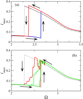
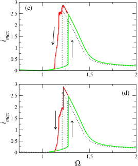
Figure 15: Induced total current amplitude $i_{max}$ as a function of the driving frequency $\Omega$ for two-dimensional $N_{x}\times N_{y}$ SQUID metamaterials with $\gamma=0.002$, $\phi_{dc}=0$, and (a) $\beta=1.27$, $N_{x}=N_{y}=20$, $\phi_{ac}=0.1$, periodic boundary conditions; (b) $\beta=1.27$, $N_{x}=N_{y}=20$, $\phi_{ac}=0.1$, free-end boundary conditions; (c) $\beta=0.15$, $\phi_{ac}=0.02$, $N_{x}=N_{y}=20$, free-end boundary conditions; (d) $\beta=0.15$, $\phi_{ac}=0.02$, $N_{x}=N_{y}=40$, free-end boundary conditions. The black dotted lines indicate the corresponding $i_{max}$ vs. $\Omega$ curves for a single rf SQUID.

Typical current amplitude - frequency curves are shown in Fig. 15, in which the total current amplitude $i_{max}$ is shown as a function of the frequency $\Omega$ of the ac flux field (dc flux is set to zero). In this figure, the value of $\beta_{L}$ has been chosen so that the SQUIDs are well into the hysteretic regime ($\beta_{L}\simeq 8$). It is observed that bistability appears in a frequency band of substantial width. The corresponding curves (black-dotted) for a single SQUID are also shown for comparison. In Fig. 15a, in which periodic boundary conditions have been employed, the bistability region for the SQUID metamaterial is narrower than that for a single SQUID, although the total current amplitude is slightly larger than that for a single SQUID. For periodic boundary conditions, the size of the metamaterial does not affect those results; current amplitude - frequency curves for larger arrays with $N_{x}=N_{y}=40$ and $N_{x}=N_{y}=80$ (not shown here) are practically identical to those shown in Fig. 15a. In all the other figures till the end of this Section, free-end boundary conditions [Eqs. (71)] which are appropriate for finite-size SQUID metamaterials are assumed. In that case, the total current amplitude - frequency curves are very sensitive to the initial conditions as well as the model and numerical parameters such as the frequency increment, the scanned frequency band, etc. For an illustration, the curves shown in Fig. 15b in different colors (red and green) have been calculated using different initializations of the SQUID metamaterial. The parts of the current amplitude - frequency curves for the SQUID metamaterial which are close to those for a single SQUID are formed by almost homogeneous states, i.e., states in which all the SQUIDs are close to either the high-current amplitude or the low-current amplitude single-SQUID states. Completely homogeneous states are formed easily in periodic SQUID metamaterials, but they are destroyed by perturbations in the finite-size ones; compare Figs. 15a and 15b. In the latter figure, the observed staircase-like curve with many small steps indicates the existence of many different solutions which are formed when a number of SQUIDs are close to the high-current single-SQUID state while the others are in the low-current single-SQUID state. In Fig. 15c and d, the corresponding curves for SQUIDs with $\beta_{L}\lesssim 1$ ($\beta=0.15$) are shown. A comparison with the corresponding curves for a single SQUID (black-dotted curves) indicates that the bistability regions have nearly the same width. For the values of $\phi_{ac}$ used in Figs. 15, the nonlinearities are already substantial, and thus capable to make the total current amplitude - frequency curves significantly hysteretic. The excited nonlinearities are also evident from the shifting of the resonance frequency of the SQUID metamaterial, which should be close to $\Omega_{SQ}$ in the linear regime, to considerably lower values. Indeed, the maximum of the total current amplitude in Figs. 15c and d is at $\Omega\sim 1.2$, while the corresponding $\Omega_{SQ}$ is $\sim 1.39$.

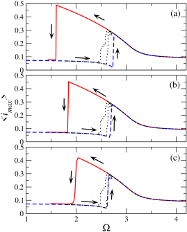
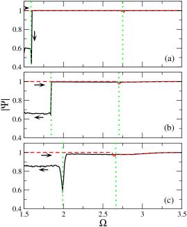
Figure 16: Left: Total current amplitude averaged over $n_{R}=30$ realizations of disorder, $<i_{max}>_{n_{R}}$, as a function of the driving frequency $\Omega$ for a SQUID metamaterial with $N_{x}=N_{y}=20$, $\alpha=0.002$, $\beta=1.27$, $\phi_{ac}=0.1$, $\phi_{dc}=0$, and (a) $\delta\beta=\pm 0.01$; (b) $\delta\beta=\pm 0.05$; (c) $\delta\beta=\pm 0.1$. Right: The corresponding magnitude of the synchronization parameter averaged over $n_{R}=30$ realizations of disorder, $<|\Psi|>_{n_{R}}$, as a function of the driving frequency $\Omega$ in the bistability region for a SQUID metamaterial with $N_{x}=N_{y}=20$, $\alpha=0.002$, $\beta=1.27$, $\delta\beta=\pm 0.01$, $\phi_{dc}=0$, $\phi_{ac}=0.1$, and (a) $\delta\beta=\pm 0.01$; (b) $\delta\beta=\pm 0.05$; (c) $\delta\beta=\pm 0.1$. The arrows indicate the direction of frequency variation while the green dotted lines the corresponding bistability intervals.

Up to this point, all the SQUIDs in a metamaterial are assumed to be identical; however, slight deviations in the values of the parameters of individual SQUIDs may occur in a SQUID metamaterial, due to unavoidable imperfections in the fabrication procedure. The existing experience shows that the available fabrication technology allows for the fabrication of SQUID metamaterials with parameter variation within a few percent from one SQUID to another (typically $1-2\%$). Thus, weak quenched disorder is present in all realizable SQUID metamaterials, that may affect their collective behavior. One possible source of disorder comes through random deviations of the critical currents $I_{c}$ of the Josephson junctions in the SQUIDs from a particular target value. Random variation of the critical current from one SQUID to another affects in turn the SQUID parameter $\beta_{L}$ of individual SQUIDs and eventually their nominal resonance frequency $\Omega_{SQ}$. There are of course other sources of disorder, which are related to the experimental apparatus and/or the procedure of measurement ²⁰²; e.g., the presence of stray magnetic fields that are created either by the magnetic components in the experimental setup or by sources from outside, such as the magnetic field of the earth. Stray magnetic fields effectively cause inhomogeneities in the applied field, so that different SQUIDs are subjected to different bias (dc) flux fields which shift randomly their resonance frequency away from its nominal value. Their effect is clearly revealed in the spoiled tunability patterns in reference ²⁰². In the rest of this Section, $\beta$ (equivalently $\beta_{L}$) is allowed to vary randomly from one SQUID to another around a target (mean) value $\Omega_{SQ}$, by a few percent. In order to make statistically meaningful predictions, statistical averages of the currents over many realizations, $n_{R}$, of disorder configurations have to be made. Remarkably, the calculations reveal that weak disorder does not destroy bistability, but, instead, it stabilizes the system against modulational or other instabilities. The robustness of the bistability region is important for prospective applications in which SQUID metamaterials could replace nonlinear resonators as read-out units for superconducting flux qubits ²¹⁸, that perform quantum non-demolishion measurements.

The effect of weak quenched disorder on the total current amplitude - frequency curves of SQUID metamaterials is shown in Fig. 16, in which the $\beta$ parameters of the SQUIDs are drawn from a uniform random distribution of zero mean. For obtaining statistically reliable results, statistical averages are calculated over $n_{R}$ realizations of quenched disorder. In the left panels of Fig. 16a, b, and c, the disorder strength on the parameter $\beta$ is $\pm 0.01$, $\pm 0.05$, and $\pm 0.1$, respectively, and $n_{R}=30$. In the left panels of Fig. 16, the stability interval of the high-current amplitude, almost homogeneous states shrinks with increasing strength of disorder. Apparently, weak disorder exhibits wider bistability as compared to the corresponding ordered case ²⁰⁴. Those results are related to earlier work on disordered networks of nonlinear oscillators in which moderate disorder may enhance synchronization and stabilize the system against chaos ^{219, 220}. Stabilization of Josephson circuits against chaos, in particular, has been recently demonstrated by numerical simulations in the time domain ²²¹. Moreover, experimental stabilization of qubit spectral resonance with random pulses has been observed ²²². In the context of SQUID metamaterials, synchronization of individual SQUIDs in the high or low current amplitude states results in high or low total current amplitude for the metamaterial as a whole. This requires that (almost) all the SQUIDs are in phase. It could be natural to assume that the more nearly identical the elements of a SQUID metamaterial are, the better their synchronization will be. However, even in the ideal case of identical elements, the earlier assumption may not be true and the in-phase state may be dynamically unstable. Then, synchronization is reduced and the SQUID metamaterial cannot remain for too long in the high total current amplitude state that is more sensitive to instability. This type of disorder-assisted self-organization may also occur by introducing local disorder in an array of otherwise identical oscillators, i.e., in the form of impurities ^{223, 224}. In this case, the impurities trigger a self-organizing process that brings the system to complete synchronization and suppression of chaotic behavior.

In order to ensure that the averaged total current amplitude - frequency curves in the left panels of Fig. 16 indeed correspond to (almost) homogeneous (uniform) states, an appropriate measure of synchronization has to be calculated. Thus, a complex synchronization parameter is defined as

$$\Psi=\left<\frac{1}{N_{x}\,N_{y}}\sum_{n,m}e^{2\pi i\phi_{n,m}}\right>_{\tau,n_{R}},$$ (72)

where the brackets $<>$ denote averaging both in time (i.e., in one oscillation period, $\tau=T$) and the number of realizations of disorder $n_{R}$. The magnitude of $\Psi$ quantifies the degree of synchronization between the SQUIDs; $|\Psi|$ may vary between $0$ and $1$, corresponding to completely asynchronous and synchronized states, respectively. The calculated values of $|\Psi|$ for (parts of) the averaged total current amplitude-frequency are shown in the right panels of Fig. 16 for strongly driven SQUID metamaterial and three different levels of disorder. The bistability regions shrinks with increasing strength of disorder (from top to bottom); the parameter $|\Psi|$ for the low current amplitude states remains close to unity for the whole range of frequencies shown. That parameter for the high current amplitude states exhibits similar behavior within the bistability region; however, as soon as the frequency reaches the lower boundary of the bistability region, the high current amplitude states start losing their stability and the synchronization breaks down. Thus, for frequencies below the left green (dotted) vertical line, the SQUID metamaterial has settled to a low current amplitude state which however preserve some degree of synchronization.

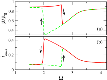
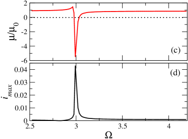
Figure 17: Relative magnetic permeability $\mu_{r}=\mu/\mu_{0}$ for the low and high current amplitude states as a function of the driving frequency $\Omega$, for a disordered SQUID metamaterial with $N_{x}=N_{y}=20$, $\gamma=0.002$, $\beta=1.27$, $\phi_{dc}=0$, and (a) $\delta\beta=\pm 0.1$, $\phi_{ac}=0.1$; (c) $\delta\beta=\pm 0.01$, $\phi_{ac}=0.001$. The corresponding total current amplitude - frequency curves are shown in (b) and (d), respectively. Multiple-valued magnetic response is observed in the bistability region of (a). Negative $\mu_{r}$ is observed in (c) within a narrow frequency band just above the resonance frequency. The parameters of (a) and (b) are the same with those in Fig. 16c (left panels).

The magnetic response of the SQUID metamaterial at any particular state can be calculated in terms of the magnetization using simple electrical equivalent circuit models ^{133, 118, 134}. Assuming for simplicity a tetragonal unit cell ($d_{x}=d_{y}=d$) with isotropic interactions between neighboring SQUIDs ($\lambda_{x}=\lambda_{y}\equiv\lambda$), and a squared SQUID area of side $\alpha$, the magnetization is

$$M=\frac{\alpha^{2}<I>}{d^{2}D},$$ (73)

where $<I>=I_{c}\,<i>\equiv I_{c}\frac{1}{N_{x}N_{y}}\sum_{n,m}<i_{n,m}>_{\tau}$ is the spatially and temporally averaged current in the SQUID. Note that SQUID metamaterials fabrication technology is currently planar, while the magnetization is defined to be inversely proportional to a unit volume. However, the experiments on SQUID metamaterials currently involve waveguides, in which the samples are placed. Thus, the necessary third dimension, which enters into the expression for the magnetization Eq. (73), comes from the length of the waveguide cavity in the direction that is perpendicular to the SQUID metamaterial plane $D$ ^{118, 34, 202, 134}. Using fundamental relations of electromagnetism, the relative magnetic permeability can be written as

$$\mu_{r}=1+\frac{M}{H},$$ (74)

where $H$ is the intensity of a spatially uniform magnetic field applied perpendicularly to the SQUID metamaterial plane. The latter is related to the external flux applied to the SQUIDs through

$$H=\frac{\Phi_{0}}{\mu_{0}\alpha^{2}}<\phi_{ext}>,$$ (75)

where $\mu_{0}$ is the magnetic permeability of the vacuum, and the brackets denote temporal averaging. Combining Eqs. (73)-(75), we get

$$\mu_{r}=1+\kappa\frac{<i>}{<\phi_{ext}>},$$ (76)

where the coefficient $\kappa=\frac{\mu_{0}\alpha I_{c}}{\Phi_{0}}\frac{\alpha^{3}}{d^{2}D}$ is the analogue of the filling factor in the context of conventional metamaterials. For a rough estimation of the constant $\kappa$ we assume that $L\sim\mu_{0}\alpha$, where $L$ is the SQUID self-inductance, and that $D\simeq d$. Then, we have that $\kappa\sim\beta\left(\frac{\alpha}{d}\right)^{3}$. Using $\alpha=d/2$ and $\beta=1.27$ we get $\kappa\simeq 0.16$.

While the expression for the magnetic permeability is rather simple, there is some uncertainty about the value of the factor $\kappa$. However, for a reasonable value of $\kappa$ the magnetic permeability can be negative within a narrow frequency band above the single-SQUID resonance frequency for weakly driven SQUID metamaterials. In that case, increasing disorder results in weakening the negative response of the metamaterial; thus, for relatively strong disorder the response is not sufficient to provide negative $\mu_{r}$ even for strongly driven SQUID metamaterials, as can be seen in Fig. 17a. In that figure it is also observed that due to the bistability, the relative magnetic permeability $\mu_{r}$ may obtain two different values depending on which state the SQUID metamaterial is. The currents $i_{n,m}$ with given $\phi_{ext}$ can be calculated from Eq. (69) when the corresponding $\phi_{n,m}$ have been calculated from Eq. (48). Then, Eq. (76) provides $\mu_{r}$ for a particular, parameter-dependent $\kappa$ coefficient. Thus, simultaneously stable SQUID metamaterial states exhibit different magnetic responses to an external magnetic field and therefore exhibit different values of $\mu_{r}$. Such magnetic multi-response in the presence of disorder is observed in Fig. 17a, with the corresponding $<i_{max}>_{n_{R}}-\Omega$ curves shown in Fig. 17b. The same quantities are shown in Fig. 17c and d, respectively, for a weakly driven SQUID metamaterial and lower strength of disorder. Here, $\beta$ varies randomly by $\pm 0.1$ ($~{}8\%$) around the nominal value $\beta=1.27$. The nonlinear effects become unimportant bringing the metamaterial close to the linear limit, and the hysteresis in the $<i_{max}>_{n_{R}}-\Omega$ curve as well as in the $\mu_{r}-\Omega$ curve dissappears. Note that the behavior of $\mu_{r}$ follows closely that of the averaged total current amplitude $<i_{max}>_{n_{R}}$. Furthermore, at driving frequencies below (but very close to) the single-SQUID resonance in the linear regime $\Omega_{SQ}\simeq 3$ ($\beta=1.27$), the SQUID metamaterial becomes strongly diamagnetic, so that it actually crosses the zero $\mu_{r}$ line. Such extreme diamagnetism corresponds to negative $\mu_{r}$, which persists within a narrow frequency band, just like in conventional metamaterials. Similar calculations with a transmission line model fed by experimental transmission data, produce qualitatively similar results ³⁴.

3 SQUID-Based Metamaterials II: Localization and Novel Dynamic States

3.1 Intrinsic Localization in Hamiltonian and Dissipative Systems

Discrete breathers (DBs), also known as intrinsic localized modes (ILMs), are spatially localized and time-periodic excitations which appear generically in extended periodic discrete systems of weakly coupled nonlinear oscillators ^{225, 226, 227, 228}. DBs may be generated spontaneously as a result of fluctuations ^{229, 230}, disorder ²³¹, or by purely deterministic mechanisms ^{232, 233, 234}. Since their discovery ²³⁵, in a large volume of analytical and numerical studies the conditions for their existence and their properties have been explored for a variety of nonlinear mathematical models of physical systems. Their very existence has been proved rigorously for both energy-conserving (Hamiltonian) and dissipative lattices ^{236, 237}, and several numerical algorithms have been designed for their accurate construction ^{238, 239, 240, 241}. A fundamental requirement for their existence is that their frequency of oscillation and its multitudes are outside the linear frequency band. Importantly, they have been observed in a variety of physical systems, such as solid state mixed-valence transition metal complexes ²⁴², quasi-one dimensional antiferromagnetic chains ²⁴³, arrays and ladders of Josephson junctions ^{244, 245, 246, 247}, micromechanical cantilever arrays ²⁴⁸, optical waveguide systems ²⁴⁹, layered crystal insulator at $300K$ ²⁵⁰, and proteins ²⁵¹. Further experiments concerning breathers in crystals are reviewed in Ref. ²²⁸. Once generated, DBs modify system properties such as lattice thermodynamics and introduce the possibility of nondispersive energy transport ^{252, 253}, because of their potential for translatory motion (i.e., mobility) along the lattice ²⁵⁴. In numerical experiments, DB mobility can be achieved by applying appropriate perturbations ²⁵⁵. From the perspective of applications to experimental situations where dissipation is always present, dissipative DB excitations (usually driven by a sinusoidal power source) are more relevant than their energy-conserved (Hamiltonian) counterparts. Dissipative DBs, which possess the character of an attractor for initial conditions in the corresponding basin of attraction, are generated whenever power balance, instead of the conservation of energy, governs the dynamics of the nonlinear lattice. Furthermore, the attractor character of dissipative DBs allows for the existence of quasi-periodic and even chaotic DBs ^{256, 257}.

3.2 Dissipative Breathers in SQUID Metamaterials

The existence of dissipative DBs has been numerically demonstrated in conventional (metallic) metamaterials comprising split-ring resonators, both in the ”bulk” and the ”surface” (i.e., in the ends and the edges, respectively, of one- and two-dimensional finite systems) ^{258, 259, 260, 261}, as well as in binary metamaterial models ^{262, 263}. In typical experimental situations, SQUID metamaterials are driven by an ac (sinusoidal) flux field and they are subjected to dissipation, mainly due to quasi-particle tunneling through the Josephson junction. Their discreteness, along with weak coupling between their elements and the (Josephson) nonlinearity, favors the appearence of dissipative breathers. Moreover, due to low dissipation in SQUID metamaterials, dissipative breathers in those systems could be in principle observed experimentally through advanced imaging techniques such as the Laser Scanning Microscopy (LSM) ²⁶⁴. Here, the existence of dissipative DBs in SQUID metamaterials is demonstrated in the one-dimensional case, for simplicity and ease of presentation; however, it has been demonstrated that increasing dimensionality does not destroy breather excitations either in conventional or SQUID metamaterials ^{163, 207}. In SQUID metamaterials, dissipative DBs can be generated either by properly designed their initial state, or by driving them through a stage of modulational instability; the latter method allows for spontaneous formation of dissipative DBs. Since the SQUIDs in a metamaterial are weakly coupled (through magnetic dipole-dipole forces), the breather structures which are generated with either of these two methods are highly localized; thus, a large amount of the energy provided initially to the SQUID metamaterial is concentrated in only a few SQUIDs. The generation and subsequent evolution of dissipative DBs can thus be visualized on three-dimensional plots in which the fluxes through the SQUIDs or the currents in the SQUIDs are plotted on the lattice site $n$ - time $\tau$ plane. In order to generate DBs by initialization, a trivial breather configuration has to be constructed first, which corresponds to a numerically accurate solution in the case of vanishing coupling between SQUIDs (anti-continuous limit ²³⁸). Then, using one of the several breather-finding algorithms, a DB family can be obtained by slowly increasing the coupling coefficient, say $\lambda$. That family has a member-breather for each value of $\lambda$ up to a critical one $\lambda_{c}$ that depends on the other parameters of the system; for $\lambda>\lambda_{c}$ the DB family destabilizes and dissapears. In order to construct a trivial dissipative DB configuration, sufficiently strong nonlinearity is required for the individual SQUIDs to exhibit multistability; for that purpose, one first calculates the flux amplitude $\phi_{max}$ - driving frequency $\Omega$ curve of the single SQUID. For a particular frequency $\Omega$ in the multistability region, at least two simultaneously stable solutions of the single SQUID (all the SQUIDs are regarded to be identical) have to be identified, say $(\phi_{0},\dot{\phi_{0}}$ ($0$) and $(\phi_{1},\dot{\phi_{1}}$ ($1$), with low and high flux amplitude $\phi_{max,0}$ and $\phi_{max,1}$, respectively. Then the initial state of the SQUID metamaterial is constructed by setting one of the SQUIDs, say that at $n=N/2$ in the state-solution $1$, and all the others to the state-solution $0$ ($N$ is the number of SQUIDS in the metamaterial). The SQUID at $n=N/2$ is hereafter referred to as the central DB site, which also determines its location; all the others constitute the ”background”. That configuration is used as initial condition for the integration in time of Eqs. (32) to numerically obtain a stable dissipative DB for a given value of $\lambda$. Note that one could start integrating at $\lambda=0$ and then slowly increase the value of $\lambda$ up to the desired one ($\lambda<\lambda_{c}$); however, since $\lambda\ll 1$, that continuation procedure may not be necessary. Note also that the procedure for obtaining dissipative DBs is easier than the corresponding one for obtaining Hamiltonian DBs, for which Newton’s method instead of merely numerical integration is required. In the obtained dissipative DB state, all the SQUIDs are oscillating with frequency $\Omega_{b}=\Omega$ (period-1 DBs, with their frequency being locked to that of the driving flux field $\Omega$), although their flux or current amplitudes are generally different. Note however that there may also be DBs with more complicated temporal behavior ²⁵⁶.

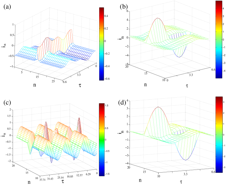
Figure 18: (a) Temporal evolution of a dissipative discrete breather during one driving period $T_{b}=2\pi/\Omega_{b}=6.6$, for $\phi_{dc}=0.5$, $\phi_{ac}=0.2$, $\beta=1.27$, $\gamma=0.001$, $\lambda=-0.1$. (b) $\&$ (d) Temporal evolution of a dissipative discrete breather during one driving period $T_{b}=2\pi/\Omega_{b}=6.6$, for $\phi_{dc}=0$, $\phi_{ac}=0.6$, $\beta=1.27$, $\gamma=0.001$, $\lambda=-0.1$. (c) Temporal evolution of a dissipative discrete breather during three driving periods $T_{b}=2\pi/\Omega_{b}=12.57$, for $\phi_{dc}=0$, $\phi_{ac}=1.2$, $\beta=1.27$, $\gamma=0.001$, $\lambda=-0.0225$. From (a) to (d), only part of the array ($N=30$) is shown for clarity.

For a metamaterial comprising hysteretic SQUIDs ($\beta_{L}>1$), there are more possibilities for constructing trivial DB configurations. Recall that for $\beta_{L}>1$, the SQUID potential has more than one minimums, with their number increasing by further increasing $\beta_{L}$. Furthermore, a dc flux bias $\phi_{dc}$ also affects the SQUID potential at will; for example, by applying a dc flux bias $\phi_{dc}=0.5$, the SQUID potential becomes a double-well one. Then, there are at least two simultaneously stable states, one with $\phi_{max}\sim 0$ and the other with $\phi_{max}\sim 1$, corresponding to the left and right minimum of the SQUID potential, respectively. Those states can be employed to construct a trivial DB configuration as described earlier. Such a double-well dissipative DB is shown in Fig. 18(a), in which the spatio-temporal evolution of the induced currents $i_{n}$ ($n=1,2,3,...,N$) is plotted during one period of the DB oscillation, $T_{b}=\frac{2\pi}{\Omega_{b}}$. The currents in both the background SQUIDs and the SQUID on the central site are oscillating with the same frequency $\Omega_{b}=\Omega$, i.e., the frequency of the driving flux field. For $\phi_{dc}=0$ but still $\beta_{L}>1$, no other DBs of that type can be obtained, since the local minimums are highly metastable; for sufficiently high ac flux amplitude $\phi_{ac}$ there may be more stable states which are generated dynamically due to strong nonlinearity. These states, which usually have high flux amplitude $\phi_{max}$ can be used to construct trivial DB configurations as described earlier. Two typical examples of such dissipative DBs, which are simultaneously stable, are shown in Fig. 18(b) and (d). This is possible because at that frequency (with corresponding period $T_{b}=6.6$) there are three simultaneously stable single-SQUID solutions; one with low flux amplitude $\phi_{max}$ and two with high flux amplitude $\phi_{max}$. Each of the high flux amplitude solutions can be combined with the low flux amplitude solution so that two trivial DB configurations can be constructed, which result in the two different dissipative DBs. The DB frequency $\Omega_{b}$ is again locked to the driving frequency $\Omega$ ($\Omega_{b}=\Omega$). For relatively weak coupling between SQUIDs, dissipative DBs can be also obtained which period of oscillation is a multiple of that of the external driver $\Omega$ (subharmonic dissipative DBs). Such a period-3 dissipative DB is shown in Fig. 18(c), in which the current in the SQUID of the central DB site apparently oscillates with $T_{b}=3T$, with $T=2\pi/\Omega$, while the currents in the background SQUIDs oscillate with $T_{b}=T$. Some remarks are here in order: a major difference between Hamiltonian and dissipative DBs is that in the former the background oscillators are at rest at all time while in the latter the background oscillators oscillate as well, although with an amplitude different than that of the oscillator at the central DB site. In Fig. 18(a), the currents in all the SQUIDs are oscillating in phase; to the contrary, in Figs. 18(b), (c), and (d), the currents in the background SQUIDs are in anti-phase with respect to the current in the SQUID of the central DB site. This has significant consequencies for the local magnetic response of the SQUID metamaterial, since the local magnetization is directly proportional to the induced current. Thus, the observed phase difference indicates that the breathers may change locally the magnetic response of the system from paramagnetic to diamagnetic or vice versa ^{163, 207}. In Figs. 18(a), (b), and (d), the time-dependence of the currents in the background SQUIDs is clearly non-sinusoidal, due to strong nonlinearities. The time-dependence of the current in the SQUID of the central DB site on the other hand seems perfectly sinusoidal, which is due to the high flux amplitude and the shape of the SQUID potential.

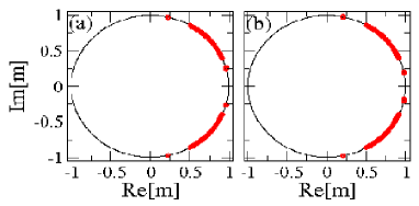
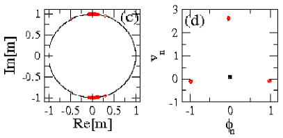
Figure 19: (a) $\&$ (b) Floquet spectra for the simultaneously stable dissipative discrete breathers shown in Fig. 18(b) and (d), respectively; all the eigenvalues lie on a circle of radius $R_{e}=\exp(-\gamma T_{b}/2)\simeq 0.996705$ in the complex plane. (c) Floquet spectra for the period-3 dissipative discrete breather shown in Fig. 18(c); all the eigenvalues lie on a circle of radius $R_{e}=\exp(-\gamma T_{b}/2)\simeq 0.993735$. (d) Reduced stroboscopic diagrams for the SQUID at the central DB site at $n=n_{b}=N/2$ (red circles), and the SQUID at $n=7$ in the background (black square), for the period-3 dissipative discrete breather shown in Fig. 18(c).

The linear stability of dissipative DBs is addressed through the eigenvalues of the Floquet matrix (Floquet multipliers). A dissipative DB is linearly stable when all its Floquet multipliers $m_{i},~{}i=1,...,2N$ lie on a circle of radius $R_{e}=\exp(-\gamma T_{b}/2)$ in the complex plane ²³⁹. All the dissipative DBs shown in Fig. 18 are linearly stable. The calculated eigenvalues for the two simultaneously stable dissipative DBs in Fig. 18(b) and (d), are shown respectively in Figs. 19(a) and (b). The Floquet spectrum for the period-3 dissipative DB in Fig. 18(c), is shown in Fig. 19(c). In Fig. 19(d), two reduced stroboscopic diagrams are shown on the ${v}_{n}-\phi_{n}$ plane, with ${v}_{n}=\dot{\phi}_{n}$ being the normalized instantaneous voltage across the Josephson junction of the $n$th SQUID. The one diagram is for the SQUID at the central DB site, i.e., at $n=n_{b}=N/2$. while the other is for a SQUID in the background, at $n=7$. Clearly, the trajectory of the SQUID at $n=n_{b}$ crosses the reduced phase space at three points (red circles), while that at $n=7$ at only one point (black square).

For generating dissipative DBs experimentally, the approach based on Marin’s algorithm ²³⁹ is not particularly useful, since it requires from the system to be initialized in a rather specific state. However, DB generation in SQUID metamaterials may be a relatively easy task whenever weak disorder is present, e.g., due to imperfections during fabrication. In a particular realization of a SQUID metamaterial, the SQUIDs are not completely identical but the values of their parameters slightly fluctuate around a mean nominal value. The parameter which is affected the most from those imperfections seems to be the critical current of the Josephson element $I_{c}$ in each SQUID, which varies exponentially with the thickness of the insulating barrier. Moreover, $I_{c}$ is proportional to the SQUID parameter $\beta_{L}$ which multiplies the nonlinear term in the SQUID flux equation and essentially determines its characteristic behavior. In order to take into account that type of disorder, the parameter $\beta=\beta_{L}/2\pi$ is allowed to vary randomly around its nominal value by $\pm 1\%$ of that value. The random numbers in the interval $[\beta-1\%,\beta+1\%]$ are drawn from a uniform distribution with mean value $\beta$. Numerical simulation of disordered SQUID metamaterials for many different configurations of disorder reveal that in most cases spontaneously generated dissipative DBs appear. In Fig. 20, the spontaneous generation of dissipative DBs is illustrated for two different configurations of disorder. In that figure, the instantaneous voltage across the Josephson junction of each SQUID $v_{n}=\dot{\phi}_{n}=\frac{d\phi_{n}}{d\tau}$ is plotted on the $\tau-n$ plane. For different configurations of disorder (while all other parameters are kept the same) a different number of dissipative DBs may appear at different locations in the metamaterial. As can be observed, the number of spontaneously generated DBs is one and three for the left and the right panel of Fig. 20, respectively. Furthermore, in the left panel, the period of voltage oscillations is twice that of the driver and that of the voltages of the SQUIDs in the background. Thus, this dissipative DB is a period-2 one.

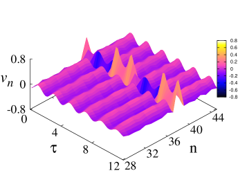
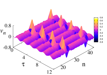
Figure 20: Spatiotemporal evolution of dissipative discrete breathers excited spontaneously in weakly disordered SQUID metamaterials during six (6) periods of the driving flux field. The voltages $v_{n}=d\phi/d\tau$ across the Josephson junctions of the SQUIDs in the metamaterial are plotted on the $\tau-n$ plane for $\phi_{dc}=0$, $\phi_{ac}=0.03$, $\beta=1.27$, $\gamma=0.001$, $\lambda=-0.0014$, $\Omega=3.11$, and $N=50$. The left and right panels correspond to different configurations of disorder, which are realized by adding to $\beta$ random numbers from a uniform distribution in the interval $[-0.01\beta,+0.01\beta]$.

3.3 Collective Counter-Intuitive Dynamic States

The investigation of networks of coupled nonlinear elements pervades all of science, from neurobiology to statistical physics, often revealing remarkable aspects of collective behavior ^{265, 266}. The effect of non-local interactions, which constitutes the ”dark corner” of nonlinear dynamics, has been extensively investigated in the last decade and has unveiled collective dynamic effects such as synchronization ^{267, 268}, pattern formation ²⁶⁹, and Turing instabilities ²⁷⁰. Recently, a dynamic state which is qualitatively distinct and it has a counter-intuitive structure, referred to in current literature as a ”chimera state”, was discovered in numerical simulations of non-locally coupled oscillator arrays ¹⁶⁷. That discovery was followed by intense theoretical ^{271, 272, 273, 274, 275, 276, 277, 278, 279, 280, 281, 282} and experimental ^{283, 284, 285, 286, 287, 288, 289, 290, 291, 292, 293, 294} activity. A chimera state is characterized by the coexistence of synchronous and asynchronous clusters (subgroups) of oscillators, even though they are coupled symmetrically and they are identical ^{295, 168}. Recent works also report on the issue of robustness of chimera states ²⁹⁶ as well as on the emergence of chimera states in systems with global ^{297, 298, 282, 299} and local coupling schemes ^{300, 166}. Chimera-like states in modular networks ^{301, 302} have been also investigated, expanding our understanding on the role of topology and dynamics for their occurrence. Further research efforts aim to stabilize chimera states by feedback schemes ³⁰³ and to control the localization of the different regimes ^{304, 305, 306}. Although chimera states are generally regarded to be metastable ^{301, 307}, or even chaotic transients ³⁰⁸, there are also examples in which they are at the global minimum of a system, such as in Ising spins in thermal equilibrium ³⁰⁹. The level of synchronization and metastability of chimera states can be quantified using measures of local and global synchronization ^{301, 307, 196}, measures of metastability ^{301, 307, 165}, the chimera index ³¹⁰, etc. Many different types of non-local interactions between the oscillators in a given network have been considered in literature, often exponentially decaying, that allow a particular system to reach a chimera state. The crucial ingredient for the emergence of chimera states is the choise of initial conditions. Those states do not actually result from destabilization of the more familiar homogeneous (i.e., synchronized) or clustered states, but they usually coexist with (some) of them. Thus, without an appropriate choice of initial condition, the system will reach one of those instead of a chimeric one. SQUID metamaterials seem to be perfect candidates for the observation of chimera states, since their constitutive elements are essentially non-locally coupled and they are highly nonlinear oscillators. Those elements (i.e., the SQUIDs) may also exhibit multistability in a frequency band around the single-SQUID resonance. As it has been discussed in the previous Section, SQUIDs are coupled magnetically through dipole-dipole forces which fall-off as the inverse cube of their center-to-center distance. That coupling, although short-ranged ³¹¹ and weak due to its magnetic nature, is clearly non-local. For simplicity, the one-dimensional non-local model, Eqs. (23), with appropriate initial conditions are used for obtaining very long-lived chimera states in SQUID metamaterials.

3.4 Chimera States in SQUID Metamaterials

3.4.1 SQUID metamaterials with non-local coupling

The one-dimensional SQUID metamaterial is initialized with

$$\phi_{n}(\tau=0)=\phi_{R},\qquad\dot{\phi}_{n}(\tau=0)=0,$$ (77)

where $\phi_{R}$ is a random number drawn from a flat, zero mean distribution in $[-\phi_{R}/2,+\phi_{R}/2]$. The following boundary conditions

$$\phi_{0}(\tau)=0,\qquad\phi_{N+1}(\tau)=0,$$ (78)

are used to account for the termination of the structure in a finite SQUID metamaterial. The degree of synchronization for the whole SQUID metamaterial or just a part of it (e.g., a cluster having $M$ SQUIDs with $M\leq N$, with $N$ being the total number of SQUIDs in the metamaterial) is quantified by the magnitude of a complex, Kuramoto-type synchronization parameter $\Psi(\tau)$, defined as

$$\Psi(\tau)=\frac{1}{M}\sum_{m=1}^{M}e^{i[2\pi\phi_{m}(\tau)]}.$$ (79)

The magnitude of that synchronization parameter, $r(\tau)=|\Psi(\tau)|$, provides a global (for the whole metamaterial) or local (within a cluster) measure of spatial coherence at time-instant $\tau$. The value of $r(\tau)$ by its definition lies in the interval $[0,1]$, where the extremal values $0$ and $1$ correspond to complete desynchronization and synchronization, respectively. The mean synchrony level $\bar{r}$, which is an index of the global synchronization level, is defined as the average of $r(\tau)$ over the total time of integration (excluding transients) ³⁰⁷, while the variance of $r(\tau)$, $\sigma_{r}^{2}$, captures how the degree of synchrony fluctuates in time. Fluctuations of the degree of synchronization have been associated with metastability and therefore $\sigma_{r}^{2}$ is indicative of the metamaterial’s metastability level ^{301, 307}.

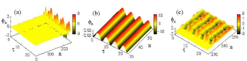
Figure 21: Spatio-temporal evolution of the normalized fluxes $\phi_{n}$ threading the SQUID rings during four driving periods $T=5.9$ for $N=256$, $\gamma=0.0022$, $\lambda_{0}=-0.05$, $\beta_{L}\simeq 0.7$, $\phi_{ac}=0.015$, and $\phi_{R}=0.85$. (a) for the whole SQUID metamaterial; (b) for part of the metamaterial that belongs to the coherent cluster; (c) for part of the metamaterial that includes the incoherent cluster.

A typical spatio-temporal flux pattern for the SQUID metamaterial, obtained after $10^{7}$ time units of time-integration, is shown in Fig. 21(a), in which the evolution of the $\phi_{n}$s is monitored during four driving periods $T=2\pi/\Omega$. In that pattern, two different domains can be distinguished, in which the fluxes through the loops of the SQUIDs are oscillating either with low or high amplitude. The enlargement of two particular sub-domains shown in Figs. 21(b) and (c), reveals the unexpected feature which characterizes a chimera state; besides the difference in the oscillation amplitudes (i.e., low-high), the two groups of SQUIDs exhibit distinctly different dynamic behaviors: the low-amplitude oscillations are completely synchronized (Fig. 21(b)) while the high-amplitude ones are desynchronized both in phase and amplitude (Fig. 21(c)). Note that since the SQUID metamaterial is driven at a particular frequency $\Omega$, there can be no net frequency drift as in phase oscillators ¹⁶⁷; instead, the period of each SQUID in the asynchronous cluster fluctuates around that of the driver, $T$.

The chimera states are very sensitive to slight changes of the model parameters, the parameters of the applied flux field(s), as well as the integration parameters such as the the time-step $\Delta\tau$ of the integration algorithm. The latter is chosen to be $0.02$, which provides reliable results for systems of nonlinear oscillators. Decreasing of the time-step (i.e., to $\Delta\tau=0.01$) leads the SQUID metamaterial to a different chimera state due to metastability effects; that state may be either more or less synchronized than the previous one, depending on the other parameters. For the parameters used in this Section, the SQUID metamaterial reaches spontaneously a chimera state for most of the initial flux density configurations with $\phi_{R}\sim\Phi_{0}$.

In Figs. 22(a) and b, the long-term spatio-temporal evolution for the fluxes $\phi_{n}$ is mapped on the $n-\tau$ plane for two different initial flux configurations (i.e., different $\phi_{R}$); the values of the $\phi_{n}$s are obtained at time-instants that are multiples of the driving period $T$, so that uniform (non-uniform) colorization indicates synchronous (asynchronous) dynamics. In Fig. 22(a), the spontaneous formation of two large clusters of SQUIDs, one with synchronized and the other with desunchronized dynamics, can be observed. More clusters of SQUIDs, two with synchronized and two with desynchronized dynamics, can be observed in Fig. 22(b), in which the effect of metastability is reflected in the sudden expansions of the upper asynchronous cluster at around $\tau\sim 0.35\times 10^{7}$ t.u. (green arrow). In the corresponding time-dependent magnitudes of the synchronization parameter averaged over the driving period $T$, $<r(\tau)>_{T}=<|\Psi(\tau)|>_{T}$, those sudden expansions correspond to jumps towards lower synchronization levels (Fig. 22(c)). Note that the same calculations, when performed using nearest-neighbor (local) coupling, result not in chimera states but instead in clustered states. The latter are also non-homogeneous states, in which two or more groups of SQUIDs are spontaneously formed; the SQUID dynamics is synchronized within each cluster, however, the clusters are not synchronized to each other. Thus, in a clustered state, $<r(\tau)>_{T}$ can be significantly lower than unity (indicating a relatively low degree of synchronization). For zero initial conditions, both the non-locally and locally coupled SQUID metamaterials result in homogeneous, competely synchronized states with $<r(\tau)|>_{T}$ practically equal to unity at all times. Typical spatial profiles of $\phi_{n}$ and the time-derivatives of the fluxes averaged over $T$, $<\dot{\phi}_{n}(\tau)>_{T}\equiv<v_{n}(\tau)>_{T}$, at the end of the integration time (at $\sim 10^{7}$ time units) of Fig. 22(a) are shown in Figs. 22(d) and (e), respectively. Note that $v_{n}(\tau)$ is the instantaneous voltage across the Josephson junction of the $n-$th SQUID, and it is the analogue of the time-derivative of the phases of the oscillators in Kuramoto-type phase oscillator models. The pattern of $<v_{n}(\tau)>_{T}$ (Fig. 22(e)) is distinctly different from the standard one for chimera states in phase oscillator models ¹⁶⁷, while it resembles the corresponding one for globally coupled, complex Ginzburg-Landau oscillators ²⁹⁸. In Figs. 22(d) and (e), synchronized clusters of SQUIDs are indicated by horizontal segments; it can be observed that besides the large incoherent cluster extending from $n=143$ to $256$, there are actually two small ones (at around $n\sim 5$ and $n\sim 112$, more clearly seen in Fig. 22(e) which are not visible in Fig. 22(d). The measure $<r(\tau)>_{T}$ as a function of $\tau$ for two different clusters of SQUIDs enclosed into the blue (small) and green (large) boxes, which exhibit synchronized and desynchronized dynamics, respectively, is shown in Fig. 22(f). The measure $<r(\tau)>_{T}$ for the synchronized cluster which extends from $n=36$ to $100$, is close to unity for all times (blue curve in Fig. 22(f)), while that for the desynchronized cluster has a significantly lower average and exhibits strong fluctuations which do not decrease with time.

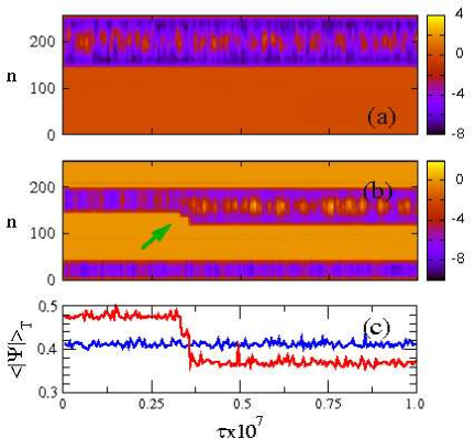
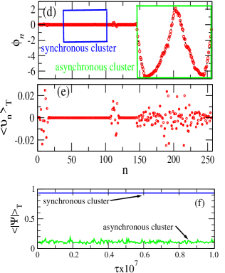
Figure 22: (a) Flux density $\phi_{n}$ as a function of site number $n$ and normalized time $\tau$ for a non-locally coupled SQUID metamaterial with $N=256$, $\gamma=0.0021$, $\lambda_{0}=-0.05$, $\beta_{L}\simeq 0.7$, and $\phi_{R}=0.9$, driven by an ac flux field of amplitude $\phi_{ac}=0.015$ and period $T=5.9$. (b) Same as (a) with $\phi_{R}=0.8$. The green arrow indicates sudden expansions of the corresponding asynchronous cluster. (c) The corresponding magnitude of the synchronization parameter averaged over the driving period $T$, $<r(\tau)>_{T}$ as a function of $\tau$; the blue and red curves are obtained for the chimera state shown in (a) and (b), respectively. (d) Spatial profile of the fluxes $\phi_{n}$ threading the SQUID rings at $\tau=10^{7}$ time units for the parameters of (a) and (b). (e) The corresponding averaged voltage profile $<v_{n}(\tau)>_{T}=<\dot{\phi}_{n}(\tau)>_{T}$. (f) The magnitude of the synchronization parameter averaged over $T$, $<r(\tau)>_{T}$, as a function of $\tau$, calculated for the coherent cluster in the small-blue box (blue curve) and for the incoherent cluster in the large-green box (green curve) in (d).

In order to determine the metastability levels of the chimera states presented in Figs. 22(a) and (b), the distributions of the values of $x\equiv<|\Psi(\tau)|>_{T}$s, $pdf(x)$, at all time-steps taken during the simulation period (excluding transients, see below) can be calculated (Fig. 23(a)). A transient period of $100T$ ($\sim 5900$ time units) was allowed, for which the data were discarded. Consider first the black-solid curves in the figure, which are actually not symmetric but they fit well to an empirical skewed Gaussian function of the form ³¹²

$$pdf(x)=pdf_{m}\exp\left\{-\ln(2)\left[\frac{1}{b}\ln\left(1+\frac{2b(x-x_{m})}{D}\right)\right]^{2}\right\},$$ (80)

where $pdf_{m}=pdf(x_{m})$ is the maximum of the distribution, $x_{m}$ is the value of $x$ at which the maximum of the distribution occurs, $b$ is the asymmetry parameter, and $D$ is related to the full-width half-maximum (FWHM) of the distribution, $W$, by

$$W=D\frac{\sinh(b)}{b}.$$ (81)

The green-dotted curve in Fig. 23(a) is a fit of the black-solid distribution with $b=0.37$ and $D=0.0116$, while $pdf_{m}$ and $x_{m}$ are taken from the calculated distribution. That fit gives $W\simeq 0.012$ for the non-locally coupled SQUID metamaterial. For the quantification of the metastability level, the FWHM of the distribution is used here (which for a symmetric Gaussian distribution is directly proportional to the standard deviation $\sigma_{r}$, and thus $W$ is proportional to the variance $\sigma_{r}^{2}$ which is a measure of the metastability level). The corresponding $pdf_{m}$ for non-homogeneous (clustered) states in locally coupled SQUID metamaterials are effectivelly $\delta-$functions, and the corresponding $W$s are smaller by more than two orders of magnitude, indicating the high metastability level of the chimera states compared to that of the clustered states. The difference in the dynamic behavior between SQUIDs in synchronized and desynchronized clusters is also revealed in the power spectra of $\phi_{n}(\tau)$. Two such spectra for frequencies around the fundamental (driving) one are shown in semi-logarithmic scale in Fig. 23(b), the one for a SQUID in the synchronized cluster ($n=40$) and the other in the desynchronized cluster ($n=190$). Note that for the chosen parameters, the resonance frequency of individual SQUIDs is at $\Omega_{SQ}\simeq 1.3$, while the linear band of the SQUID metamaterial extends from $\Omega_{min}\simeq 1.27$ to $\Omega_{max}\simeq 1.35$. The driving frequency is $\Omega\simeq 1.06$, well below the lower bound of the linear spectrum, $\Omega_{min}$. The spectrum for the SQUID at $n=40$ (black curve) exhibits very low noise levels and a strong peak at the driving frequency $\Omega$. The smaller peaks in the spectrum of the $n=40$ SQUID are also part of it, and they are located at frequencies within the linear band of the SQUID metamaterial, i.e., within the range $[\Omega_{min},\Omega_{max}]$. The longer arrow at right points at the resonance frequency (the eigenfrequency) of individual SQUIDs. Note that only a small number of the eigenfrequencies of the SQUID metamaterial are excited in that spectrum, which seem to be selected by random processes. To the contrary, the spectrum for the SQUID at $n=190$ exhibits significant fluctuations, the peak at the driving frequency, and in addition to that a frequency region around $\Omega\sim 0.9-1.05$ in which the average fluctuation level remains approximatelly constant, forming a shoulder that often appears in such spectra for SQUIDs in desynchronized clusters of chimera states.

Figure 23: (a) The distributions (divided by their maximum value) of $<|\Psi(\tau)|>_{T}$s at all instants of the simulation period ($\sim 10^{7}$ time units with time-step $\Delta t=0.02$) for the states shown in Fig. 22(a) and b (black-solid and red-dashed curve, respectivelly). The green-dotted curve is a fit with Eq. (80). (b) The power spectrums of $\phi_{n}(\tau)$ in semi-logarithmic scale for the SQUIDs with $n=40$ and $n=190$ that belong to the synchronized (black curve) and the desynchronized (red curve) cluster, respectively, of Fig. 22(a). The arrow at right points at the eigenfrequency of individual SQUIDs, $\Omega_{SQ}\simeq 1.3$.

More chimera states, emerging from a variety of initial conditions along with the corresponding local synchronization parameter $|Z_{n}|$ are shown in the left and right panels, respectively, of Fig. 24. The real-valued local synchronization parameter $|Z_{n}|$ is a measure that can be calculated for a group of $2\delta$ coupled oscillators (a sub-system of a larger system of $N$ coupled oscillators) at every instant of time. Its value indicates the instantaneous degree of spatial coherence, i.e., the instantaneous degree of synchronization, of that group. Is is defined as the magnitude of the complex parameter ²⁷⁷

$$Z_{n}=\frac{1}{2\delta}\sum_{|m-n|\leq\delta}e^{2\pi i\phi_{m}},\quad n=\delta+1,\dots,N-\delta.$$ (82)

A value of the local order parameter $|Z_{n}|=1$ ($|Z_{n}|<1$) indicates that the $n-$th oscillator belongs to a synchronized (desynchronized) cluster of the system of $N$ oscillators. For a finite system of $N$ coupled oscillators such as the SQUID metamaterial considered here (i.e., whose boundary conditions are not periodic), Eq. (82) holds for the oscillators whose indices run from $n=\delta+1$ to $N-\delta$. For the oscillators close to the boundaries of the structure, the calculation of the local order parameter has to be modified as follows

$$Z_{n}=\frac{1}{\delta}\sum\limits_{m=n}^{n+\delta}e^{i2\pi\phi_{m}},~{}~{}~{}{\rm for}~{}~{}~{}n=1,\dots,\delta,$$ (83)

and

$$Z_{n}=\frac{1}{\delta}\sum\limits_{m=n-\delta}^{n}e^{i2\pi\phi_{m}},~{}~{}~{}{\rm for}~{}~{}~{}N-\delta+1,\dots,N.$$ (84)

Here the local order parameter is employed to quantufy locally the degree of synchronization of the collective states obtained for the SQUID metamaterial. In the spatiotemporal flux patterns shown in the left panels of Fig. 24, the values of the $\phi_{n}$s are obtained at time-instants that are multiples of the driving period $T=2\pi/\Omega$ of the ac flux field. In particular, Figs. 24(a) and (c) correspond to typical chimera patterns which exhibit a cluster of desynchronized SQUIDs. In Fig. 24(a) this cluster is small and it is located around $n=150$, while in Fig. 24(c) it is much larger, spanning the region from $n\simeq 70$ to $n\simeq 190$. The SQUIDs which do not belong to these clusters are not all synchronized to each other. Instead, small sub-clusters of SQUIDs are apparent as stripes with uniform colorization. The SQUIDs that belong to such a stripe are synchronized; however, the stripes are not synchronized to each other. Furthermore, the flux oscillations in the SQUIDs that belong to the desynchronized clusters are much stronger than those in the other SQUIDs. In Figs. 24(b) and (d), chimera states exhibitng two desynchronized clusters are shown. In Fig. 24(b) these two clusters are small and they are located around $n\simeq 80$ and $n\simeq 160$. In Fig. 24(d), on the other hand, the two desynchronized clusters are so large that do not leave any space for any synchronized cluster to exist. A drifting pattern can be observed in Fig. 24(e), in which the largest part of the SQUID metamaterial forms a desynchronized cluster which size and position vary in time. Finally, Fig. 24(f) demonstrates a pattern of low-amplitude flux oscillations with multiple so-called solitary states ³¹³, where many SQUIDs have escaped from the main synchronized cluster and perform oscillations of higher amplitudes (depicted by the light green stripes in the otherwise orange background). The degree of synchronization within the aforementioned states is visualized through the corresponding space-time plots of the local synchronization parameter, Eqs. (82) - (84), which are shown in the right panels of Fig. 24. Red-orange colors denote the synchronized or coherent regions and blue-green colors the desynchronized or incoherent ones. These plots reveal the complexity of the synchronization levels in the SQUID metamaterial: For example in Fig. 24(a) (right panels) it can be seen that the incoherent region located in the center of the metamaterial achieves periodically high values of synchronization demonstrated by the orange ‘”islands” within the cluster. This is related to metastability, which was also investigated in reference ¹⁶⁵. In the coherent cluster, on the other hand, blue stripes of low synchronization are observed, indicating solitary states. Note that periodic synchronization, characterized by periodic variation of the synchronization parameter, has been previously observed in phase oscillator models with external periodic driving both with and without an inertial term ^{314, 315}.

The calculation of the global synchronization parameter averaged over the steady-state integration time, $<r>_{\Delta\tau}$ in a physically relevant region of the parameter space of driving frequency $f$ and dc bias flux $\phi_{ext}=\phi_{dc}$, reveals the possibility of synchronization-desynchronization transitions in SQUID metamaterials with non-local coupling. Note that the SQUID metamaterial is initialized with zero $\phi_{n}$ and $\dot{\phi}_{n}$ at each point of the parameter plane. In Fig. 25(a)-(c), three maps of $<r>_{\Delta\tau}$ are shown on the $f-\phi_{dc}$ plane for relatively strong ac driving flux amplitude $\phi_{ac}=0.05$ and three values of the coupling coefficient $\lambda=-0.01$ (a), $-0.03$ (b), and $-0.05$ (c), for a two-dimensional tetragonal $27\times 27$ SQUID metamaterial. The frequency $f$ is given in natural units (GHz), while the single SQUID resonance frequency is $f=f_{SQ}=22.6~{}GHz$ ¹³⁴. As can be seen in the corresponding colorbars, for that value of $\phi_{ac}$ and strong coupling coefficient ($\lambda=-0.05$, Fig. 25(c)), the synchronization parameter $<r>_{\Delta\tau}$ assumes very low values in some regions of the parameter plane. Those regions are located around $\phi_{dc}=\pm 1/4$ in units of $\Phi_{0}$. From Fig. 25(c), two values of $\phi_{dc}$ close to $1/4$ are selected, and the corresponding $<r>_{\Delta\tau}$ as a function of the driving frequency $f$ are plotted in Fig. 25(d). Both curves (black and red) exhibit similar behavior; for low $f$ the metamaterial is completely synchronized with $<r>_{\Delta\tau}=1$. At $f\simeq 14.8~{}GHz$ and $f\simeq 15.2~{}GHz$ (black and red curve, respectively), $<r>_{\Delta\tau}$ begins dropping to lower values until it reaches a minimum at around $\sim 0.1$. That drop signifies a synchronization to desynchronization transition of the SQUID metamaterial with the most desynchronized state being observed at $f\sim 16.8~{}GHz$ for both curves. For further increasing frequencies, the value of $<r>_{\Delta\tau}$ increases gradually until reaching the value of unity ($<r>_{\Delta\tau}=1$) where the SQUID metamaterial has return to a completely synchronized state. Note that in that desynchronization to synchronization transition, the two curves follow closely each other. Similar synchronization to desynchronization transitions have been observed in arrays of Josephson junctions ³¹⁶. In the inset of Fig. 25(d), the time-dependence of the instantaneous value of the synchronization parameter $r(\tau)$ is shown for $f=16.8~{}GHz$, i.e., the value of $f$ for which $<r>_{\Delta\tau}$ is the lowest. It is observed that the SQUID metamaterial remains synchronized for only about $25$ time units, and then $<r>_{\Delta\tau}$ starts oscillating strongly while its average value falls rapidly. In fact, in about $100$ time units, $<r>_{\Delta\tau}$ has already reached its lowest value. Note that the minimum value of $<r>_{\Delta\tau}$ cannot be zero since the system is finite. As shown in the inset, however, the instantaneous value of $r(\tau)$ can actually reach values close to zero. The minimum value of $<r>_{\Delta\tau}$ decreases with increasing system size, while it vanishes in the ”thermodynamic limit”, i.e., for a very large SQUID metamaterial.

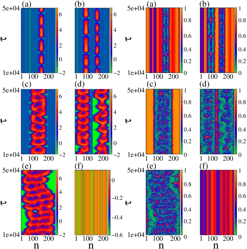
Figure 24: Left: Space-time plots for the flux density $\phi_{n}$ of the SQUID metamaterial for different initial conditions. Panels (a) and (c) show chimera states with one desynchronized region, panels (b) and (d) show chimera states with two desynchronized regions, while panel (e) show a state with a drifting desynchronized domain, and panel (f) shows a pattern with solitary states. Right: The corresponding space-time plots for the local order parameter $|Z_{n}|$ for the states shown in the left panels. Parameter values are: $T=5.9$, $N=256$, $\gamma=0.0021$, $\lambda_{0}=-0.05$, $\beta_{L}\simeq 0.7$, $\phi_{ac}=0.015$, $\phi_{dc}=0.0$.

3.4.2 SQUID metamaterials with local coupling

Chimera states have mostly been found for non-local coupling between the coupled oscillators. This fact has given rise to a general notion that non-local coupling, is an essential ingredient for their existence. However, recently, it has been demonstrated that chimeras can be achieved for global coupling as well ^{297, 298, 282, 299}. The case of local coupling (i.e., only nearest-neighbor interactions between the oscillators) has been studied less. In reference ³⁰⁰, chimera states were found in locally coupled networks, but the oscillators in the systems under consideration were not completely identical. Very recently, the emergence of single- and double-headed chimera states in neural oscillator networks with local coupling has been reported ³¹⁷. That system, however, is known to exhibit high metastability, which renders the chimera state non-stationary when tracked in long time intervals ³⁰². The emergence of multi-clustered robust chimera states in locally coupled SQUID metamaterials can be demonstrated in a relevant parameter region which has been determined experimentally ^{134, 161}. Fig. 26 shows time-snapshots of the fluxes $\phi_{n}$ for different initial conditions and for two values of the loss coefficient $\gamma$ which differ by an order of magnitude. The left panel is for $\gamma=0.024$. The initial ”sine wave” flux distribution for each simulation is shown by the gray solid line. The SQUIDs that are prepared at lower values form the coherent clusters of the chimera state, while those that are initially set at higher flux values oscillate incoherently. Moreover, as the ”wavelength” of the initial flux distribution increases, so does the chimera state multiplicity, i.e., the number of coherent and/or incoherent regions. Similar behavior is observed for lower values of the loss coefficient $\gamma=0.0024$ as shown in the right panel of Fig. 26. Here, the incoherent clusters are better illustrated since they are approximately of equal size and do not contain oscillators that ”escape” from the incoherent cluster abiding around low magnetic flux values, something which is visible in the left panel. Furthermore, the coherent clusters (emphasized by the blue solid lines) are fixed around $\phi=0$, unlike in the left panel where additional clusters located at slightly higher values also form. Here we must recall that the snaking resonance curve of a single SQUID increases significantly its winding with decreasing values of $\gamma$ (right panel), creating thus new branches of stable (and equally unstable) periodic (period-1) solutions.

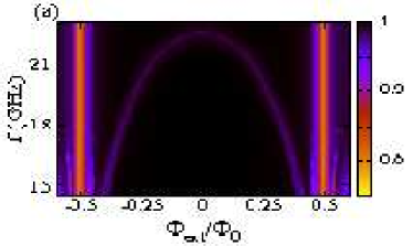
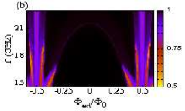
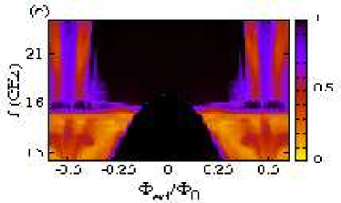
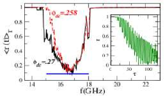
Figure 25: The magnitude of the global synchronization parameter averaged over the steady-state integration time $<r>_{\Delta\tau}$ mapped as a function of the driving frequency $f$ and the dc flux bias $\phi_{ext}=\phi_{dc}$, for a $27\times 27$ SQUID metamaterial with $\gamma=0.024$, $\beta_{L}=0.88$, $\phi_{ac}=0.05$, and (a) $\lambda_{0}=-0.01$; (b) $\lambda_{0}=-0.03$; (c) $\lambda_{0}=-0.05$. In (d), $<r>_{\Delta\tau}$ is plotted as a function of $f$ for $\phi_{dc}=0.27$ (black curve) and $\phi_{dc}=0.258$ (red curve). Inset: the instantaneous value of $r$ is shown as a function of time $\tau$ for $\phi_{dc}=0.258$ and $f=16.8~{}GHz$.

These branches are larger in number and smaller in size compared to those of higher $\gamma$ values (left panel). The lower amplitude branches which are the biggest ones attract the SQUIDs that eventually form the coherent clusters. The other SQUIDs have a plethora of higher flux amplitude states to choose from and, therefore, create a more chaotic incoherent cluster than in the case of higher $\gamma$ values. The observed chimera states can be quantified again through the local synchronization parameter $|Z_{n}|$ ¹⁹⁶, which is a measure for local synchronization. A spatial average with a window size of $\delta=5$ elements, can be employed. In the left panel of Fig. 27 the space-time plots of $|Z_{n}|$ corresponding to the chimera states of Figs. 26(a)-(d) are shown. The number of (in)coherent regions increases according to the number of half-wavelengths in the initial conditions and the size and location of the clusters is constant in time. Previous works on SQUID metamaterials demonstrated that for nonlocal coupling, single- and double-headed chimera states coexist with solitary states ³¹⁸ and metastable states of drifting (in)coherence, in a dynamical area of the SQUID metamaterial in which the driving frequency lied outside the multistability regime ^{165, 196}. For a suitable choice of the driving frequency $\Omega$, stable chimera states can be achieved for non-local coupling as well. However, those chimera states exist only for low coupling strengths $\lambda$; the threshold value of the coupling strength in the case of local coupling is much higher. Local coupling is therefore crucial for the emergence of robust chimera states, both in structure and in lifetime, for large areas of parameter space.

In the previous paragraphs, the importance of multistability and the impact of the dissipation coefficient $\gamma$ in the formation of chimera states in SQUID metamaterials was stressed. In addition to that, it is important to note the role of the network topology which is defined through the local nature of interactions and the coupling strength $\lambda$. As already shown in Fig. 26, SQUID metamaterials exhibit a variety of coexisting multi-clustered chimera states. A systematic study in the $(\lambda,\gamma)$ parameter space is depicted in the right panel of Fig. 27, in which the observed patterns for the initial conditions of Figs. 26(a)/(a’) and b/b’ are mapped out. The numbers in the brackets correspond to the multiplicity of the respective chimera states and ”synch” denotes the synchronized states. The black and white asterisk mark the $(\lambda,\gamma)$ values used in the left and right panel of Fig. 26, respectively. For low coupling strengths, single- and four-headed chimera states exist but only for low values of $\gamma$. As $\gamma$ increases, the effect of multistability diminishes and the system enters the synchronized state. As the coupling $\lambda$ becomes stronger, the synchronization threshold for $\gamma$ is shifted to higher values, below which three-headed chimeras coexist with single-headed ones. The latter persist for even higher $\lambda$ and $\gamma$ values and at the same time double-headed chimeras appear as well. For initial conditions with a larger modification in space (like in Figs. 26(c)/(c’) and (d)/(d’)), chimera states with higher multiplicity may emerge, but the mechanism towards synchronization is the same: By increasing $\gamma$, the multiplicity of the chimera state decreases and eventually the fully coherent state is reached through the appearance of solitary states ^{318, 196}.

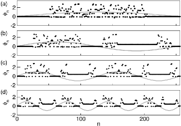
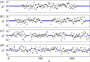
Figure 26: Snapshots of the magnetic flux density $\phi_{n}$ at time $\tau=5000$ time units for two different values of the loss coefficient: $\gamma=0.024$ in (a)-(d) and $\gamma=0.0024$ in (a’)-(d’). Grey solid lines mark the initial magnetic flux distribution used in the simulations. Blue solid lines in the right panel emphasize the coherent clusters of the chimera states. The other parameters are $T=6.24$ ($\Omega\simeq 1.007$), $\beta_{L}=0.86$,and $\phi_{ac}=0.06$.

Single-headed chimera states with very long life-times can be also obtained generically in SQUID metamaterials with nearest-neighbor coupling using initial conditions of the form $\phi_{n}(\tau=0)=-1.7$ and $\dot{\phi}_{n}(\tau=0)=+1$ for $n$ in $[n_{\ell},n_{r}]=[128,384]$ and zero otherwise, or as $\phi_{n}(\tau=0)=3+\phi_{R}$ and $\dot{\phi}_{n}(\tau=0)=\phi_{R}$ for $n$ in $[n_{\ell},n_{r}]=[128,384]$ and zero otherwise, with $\phi_{R}$ drawn from a flat, zero mean distribution in $[-4,+4]$. There is nothing special about those particular initial conditions; however, different sets of initial conditions result in different chimera states. The obtained chimeric patterns are shown in Fig. 28(a) and (b), respectively, for those initial conditions, respectively. The average over a driving period $T$ of the voltages in the Josephson junctions of the SQUIDs, $<\dot{\phi}_{n}>_{T}$, are mapped onto the $n-\tau$ plane so that uniform colorization indicates synchronized dynamics (for which the fluxes execute low amplitude oscillations). In the region of desynchronized dynamics in the interval $[n_{\ell},n_{r}]$, one can still distinguish a few small synchronized clusters that break it into several subclusters. The voltage oscillations in the desynchronized clusters differ both in amplitude and phase, since the SQUIDs there are close to or in a chaotic state. The profile of the fluxes $\phi_{n}$ threading the SQUID loops for the chimera state in Fig. 28(a) is shown in Fig. 28(c) at the end of the integration time. The desynchronized region is indicated by the seemingly randomly scattered points in the interval $[n_{\ell},n_{r}]$. The emergence of chimera states in SQUID metamaterials can be clearly attributed to the extreme multistability around the geometrical resonance frequency of individual SQUIDs, which leads to attractor crowding ¹⁹³ accompanied by the generation of several chaotic states. Thus, with proper choise of initial conditions, a large number of SQUIDs may find themselves in a chaotic state forming thus one (or more) desynchronized cluster(s). Moreover, there are also periodic states in this frequency region which are highly metastable due to attractor crowding that shrinks their basins of attraction. Thus, the flux in some of the SQUID oscillators may jump irregularly from one periodic state to another resulting in effectively random dynamics.

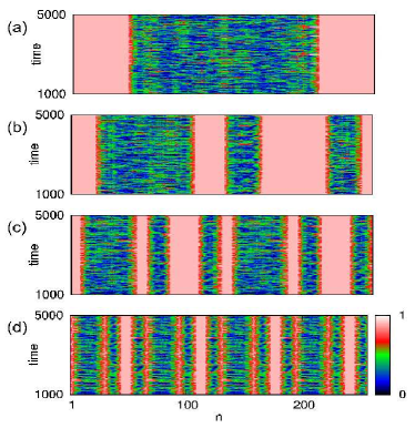
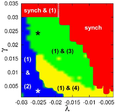
Figure 27: Left panel: Space-time plots for the magnitude of the local synchronization parameter $|Z_{n}|$ of the chimera states corresponding to Fig. 26(a), (b), (c), and (d). Right panel: Map of dynamic regimes in the $(\gamma,\lambda)$ parameter space for the initial conditions of Fig. 26(a) and (b). Numbers in brackets denote the multiplicity of the chimera state while ”synch” stands for synchronization. The other parameters are as in Fig. 26.

For the characterization of the chimera states in Figs. 28(a) and (b), except the global measure of synchronization $<r>_{T}=<|\Psi(\tau)|>_{T}$, a measure of incoherence and a chimera index are defined as follows ³¹⁰. First, we define $v_{n}(\tau)\equiv<\dot{\phi}_{n}>_{T}(\tau)$, where the angular brackets indicate average over the driving period $T$, and $\bar{v}_{n}(\tau)\equiv\frac{1}{n_{0}+1}\sum_{n=-n_{0}/2}^{+n_{0}/2}v_{n}(\tau)$ which is the local spatial average of $v_{n}(\tau)$ in a region of length $n_{0}+1$ around the site $n$ at time $\tau$ ($n_{0}<N$ is an integer). Then, the local standard deviation of $v_{n}(\tau)$ is defined as

$$\sigma_{n}(\tau)\equiv\left<\sqrt{\frac{1}{n_{0}+1}\sum_{n=-n_{0}/2}^{+n_{0}/2}\left(v_{n}-\bar{v}_{n}\right)^{2}}\right>_{n_{T}},$$ (85)

where the large angular brackets denote averaging over the number of driving periods of time-integration (excluding transients). The index of incoherence is then defined as $S=1-\frac{1}{N}\sum_{n=1}^{N}s_{n}$, where $s_{n}=\Theta(\delta-\sigma_{n})$ with $\Theta$ being the Theta function. The index $S$ takes its values in $[0,1]$, with $0$ and $1$ corresponding to synchronized and desynchronized states, respectively, while all other values in between them indicate a chimera or multi-chimera state. Finally, the chimera index is defined as $\eta=\sum_{n=1}^{N}|s_{n}-s_{n+1}|/2$ and equals to unity (an integer greater than unity) for a chimera (a multi-chimera) state. The local standard deviation $\sigma_{n}$ as a function of $n$ is shown in Fig. 28(d). Its value is practically zero in the synchronized regions, while it fluctuates between zero and unity in the desynchronized region. However, there are four small clusters indicated by the arrows in which the dynamics is synchronized. In order for these features to be visible (also apparent in Fig. 28(a)), the integer $n_{0}$ has to be close to the number of the SQUIDs that belong to the small synchronized clusters (here $n_{0}=4$). The small synchronized clusters divide the central region of the SQUID metamaterial in a number of desynchronized clusters. The indices of incoherence for the chimera states shown in Figs. 28(a) and (b), is $S=0.46$ and $S=0.44$, respectively, very close (within $1\%$) to $1-<r(\tau)>_{T}$ in both cases for a threshold value $\delta=10^{-4}$. The choice of both $n_{0}$ and $\delta$ is rather subjective, but they have to be such that the resulting indices agree with what we get by inspection. When properly chosen, however, they are very useful for comparing chimera states resulting from different initial conditions. The chimera index for the states in Figs. 28(a) and (b), is $\eta=5$ and $\eta=7$, respectively, roughly corresponding to the number of desynchronized clusters of a multi-headed chimera state. The global synchronization measure $<r(\tau)>_{T}$ as a function of $\tau$ is shown in Fig. 28(e) as black (lower) and red (upper) curve for the chimera state in Figs. 28(a) and (b), respectively. The average over all integration times (initial transients have been excluded) gives, respectively, $0.571$ and $0.59$. The strong fluctuations of these curves are a distinguishing feature of both single-headed and multi-headed chimera states; when the SQUID metamaterial is in a homogeneous or clusteres state, the size of fluctuations practically vanishes. For the obtained values of both the index of incoherence and $<r(\tau)>_{T}$ it can be concluded that the chimera state in Fig. 28(b) is slightly more synchronized than that in Fig. 28(a).

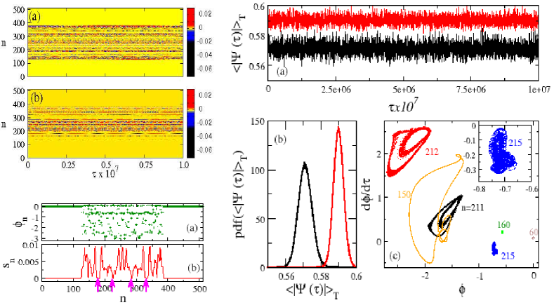
Figure 28: (a) $\&$ (b) Density plot of the fluxes $\phi_{n}$ through the SQUIDs on the $n-\tau$ plane for a SQUID metamaterial with $N=512$, $\beta_{L}=0.86$, $\gamma=0.024$, $\lambda_{0}=-0.025$, $\phi_{ac}=0.06$, and $T=6.24$ ($\Omega\simeq 1.007$), and different initial conditions (see text). (c) The flux density profile $\phi_{n}$ at $\tau=10^{7}$ time units ($\sim 1.6\times 10^{6}~{}T$ for the chimera state shown in (a). (d) The local standard deviation $\sigma_{n}$ as a function of the SQUID number $n$ for the chimera state shown in (a), for $\delta=10^{-4}$. The arrows indicate the location of small synchronized clusters. (e) The magnitude of the synchronization parameter averaged over the driving period $T$, $<r(\tau)>_{T}$, as a function of time $\tau$; the black (lower) and red (upper) curves which average to $\sim 0.571$ and $\sim 0.59$ correspond to the chimera states shown in (a) and (b), respectively. (f) The distributions of $<r(\tau)>_{T}$ with full-width half-maximum $\sim 0.0091$ and $\sim 0.0066$ for the chimera states in (a) and (b), respectively. (g) Phase portraits in the reduced, single-SQUID phase space for several SQUIDs, which number is indicated on the figure, for the chimera state in (a). Inset: Expanded phase portrait for the $n=215$ SQUID.

Moreover, their level of metastability can be estimated from the full-width half-maximum (FWHM) of the distributions of the values of $<r(\tau)>_{T}$ shown in Fig. 28(f). These distributions are well fitted to a Gaussian shape while their maximums are located at the long time averages of $<r(\tau)>_{T}$. The FWHM for the black (lower hight) and the red (higher hight) distributions turn out to be $\sim 0.57$ and $\sim 0.59$, respectively. Thus, it can be concluded that the less synchronized chimera state in Fig. 28(a) is at a higher metastability level. In Fig. 28(g), the phase portraits for several SQUIDs on the reduced single SQUID phase space $\phi_{n}-\dot{\phi}_{n}$ are shown for $n=60,150,160,211,212,215$. Those SQUIDs have been chosen because they exhibit different dynamical behaviors which ranges from periodic (i.e., the SQUID is phase locked to the driver as for e.g., $n=60$) to chaotic (e.g. for $n=212$), in which the trajectory explores a significant part of the reduced phase space.

4 SQUID Metamaterials on Lieb lattices

Besides the freedom of engineering the properties of the individual ”particles” or devices such as the SQUIDs which play the role of ”atoms” in a metamaterial, one also has the freedom to choose the arrangement of those ”particles” in space. That means that one has the freedom to choose a particular type of lattice which sites will be occupied by those ”particles”. Interestingly, there are some specific lattice geometries which give rise to novel and potentially useful frequency spectrums. Such an example is the so-called Lieb lattice. The latter is actually a square-depleted (line-centered tetragonal) lattice, described by three sites in a square unit cell as illustrated in Fig. 29(a); it is characterized by a band structure featuring a Dirac cone intersected by a topological flat band ^{319, 320}, shown in Fig. 29(b). As it is well-known, systems with a flat-band in their frequency spectrum support localized eigenmodes also called localized flat-band modes; such states have been recently successfully excited and subsequently observed in photonic Lieb lattices ^{321, 322}.

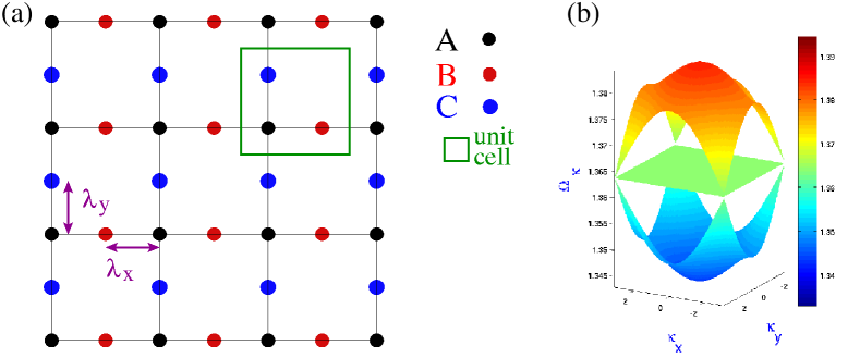
Figure 29: (a) Schematic of a Lieb lattice. The three sublattices are indicated in black (corner SQUIDs), red (edge SQUIDs), and blue (edge SQUIDs) color. The nearest-neighbor couplings $\lambda_{x}$ and $\lambda_{y}$ and the unit cell (green box) are also indicated. (b) The linear frequency spectrum $\Omega_{\bf\kappa}({\bf\kappa})$ of the SQUID Lieb metamaterial for $\beta=0.86$, and $\lambda_{x}=\lambda_{y}=-0.02$. The flat-band frequency is $\Omega_{FB}=\Omega_{SQ}\simeq 1.364$.

4.1 Nearest-Neighbor Model and Frequency Spectrum

Consider the Lieb lattice shown schematically in Fig. 29(a), in which each site is occupied by a SQUID. That SQUID Lieb Metamaterial (SLiMM) can be regarded as the combination of three sublattices indicated by different colors (black, red, blue). The SQUIDs are assumed to be identical, and they are coupled magnetically through their mutual inductances to their nearest neighbors. The dynamic equations for the fluxes through the loops of the SQUIDs are obtained from the combination of the flux-balance relations

$$\Phi_{n,m}^{A}=\Phi_{ext}+L\left\{I_{n,m}^{A}+\lambda_{x}\left[I_{n-1,m}^{B}+I_{n,m}^{B}\right]+\lambda_{y}\left[I_{n,m-1}^{C}+I_{n,m}^{C}\right]\right\},$$

$$\Phi_{n,m}^{B}=\Phi_{ext}+L\left\{I_{n,m}^{B}+\lambda_{x}\left[I_{n,m}^{A}+I_{n+1,m}^{A}\right]\right\},$$ (86)

$$\Phi_{n,m}^{C}=\Phi_{ext}+L\left\{I_{n,m}^{C}+\lambda_{y}\left[I_{n,m}^{A}+I_{n,m+1}^{A}\right]\right\},$$

where $\phi_{n,m}^{k}$ with $k=A,B,C$ is the flux through the SQUID of the $(n,m)$th unit cell of kind $k$, $I_{n,m}^{k}$ is the current in the SQUID of the $(n,m)$th unit cell of kind $k$, $\Phi_{ext}$ is the applied (external) flux, and $\lambda_{x}=M_{x}/L$ ($\lambda_{y}=M_{y}/L$) is the dimensionless coupling coefficient along the horizontal (vertical) direction, with $M_{x}$ ($M_{y}$) being the corresponding mutual inductance between neighboring SQUIDs and $L$ the self-inductance of each SQUID. The currents $I_{n,m}^{k}$ in the SQUIDS are provided by the resistively and capacitively shunted junction (RCSJ) model to be ⁹⁷

$$-I_{n,m}^{k}=C\frac{d^{2}\Phi_{n,m}^{k}}{dt^{2}}+\frac{1}{R}\frac{d\Phi_{n,m}^{k}}{dt}+I_{c}\sin\left(2\pi\frac{\Phi_{n,m}^{k}}{\Phi_{0}}\right),$$ (87)

where $R$ is the subgap resistance through the Josephson junction of each SQUID, $C$ is the capacitance of the Josephson junction of each SQUID, and $I_{c}$ is the critical current of the Josephson junction of each SQUID. From Eqs. (86) and (87), assuming that all the terms proportional to $\lambda_{x}^{a}\lambda_{y}^{b}$ with $a+b>1$ are negligible, we get ¹⁷⁰

$$LC\frac{d^{2}\Phi_{n,m}^{A}}{dt^{2}}+\frac{L}{R}\frac{d\Phi_{n,m}^{A}}{dt}+LI_{c}\sin\left(2\pi\frac{\Phi_{n,m}^{A}}{\Phi_{0}}\right)+\Phi_{n,m}^{A}=\lambda_{x}\left(\Phi_{n,m}^{B}+\Phi_{n-1,m}^{B}\right)+\lambda_{y}\left(\Phi_{n,m}^{C}+\Phi_{n,m-1}^{C}\right)+\Phi_{eff}^{A},$$

$$LC\frac{d^{2}\Phi_{n,m}^{B}}{dt^{2}}+\frac{L}{R}\frac{d\Phi_{n,m}^{B}}{dt}+LI_{c}\sin\left(2\pi\frac{\Phi_{n,m}^{B}}{\Phi_{0}}\right)+\Phi_{n,m}^{B}=\lambda_{x}\left(\Phi_{n,m}^{A}+\Phi_{n+1,m}^{A}\right)+\Phi_{eff}^{B},$$ (88)

$$LC\frac{d^{2}\Phi_{n,m}^{C}}{dt^{2}}+\frac{L}{R}\frac{d\Phi_{n,m}^{C}}{dt}+LI_{c}\sin\left(2\pi\frac{\Phi_{n,m}^{C}}{\Phi_{0}}\right)+\Phi_{n,m}^{C}=\lambda_{y}\left(\Phi_{n,m}^{A}+\Phi_{n,m+1}^{A}\right)+\Phi_{eff}^{C}.$$

where $\Phi_{eff}^{A}=[1-2(\lambda_{x}+\lambda_{y})]\Phi_{ext}$, $\Phi_{eff}^{B}=(1-2\lambda_{x})\Phi_{ext}$, and $\Phi_{eff}^{C}=(1-2\lambda_{y})\Phi_{ext}$ are the ”effective” external fluxes.

Using the relations $\tau=\omega_{LC}t$, $\phi_{n,m}^{k}=\frac{\Phi_{n,m}^{k}}{\Phi_{0}}$, and $\phi_{ext}=\frac{\Phi_{ext}}{\Phi_{0}}$, where $\omega_{LC}={1}/{\sqrt{LC}}$ is the inductive-capacitive ($LC$) SQUID frequency, the dynamic equations for the fluxes through the SQUIDs can be written in the normalized form

$$\ddot{\phi}_{n,m}^{A}+\gamma\dot{\phi}_{n,m}^{A}+\beta\sin\left(2\pi\phi_{n,m}^{A}\right)+\phi_{n,m}^{A}=\lambda_{x}\left(\phi_{n,m}^{B}+\phi_{n-1,m}^{B}\right)+\lambda_{y}\left(\phi_{n,m}^{C}+\phi_{n,m-1}^{C}\right)+[1-2(\lambda_{x}+\lambda_{y})]\phi_{ext},$$

$$\ddot{\phi}_{n,m}^{B}+\gamma\dot{\phi}_{n,m}^{B}+\beta\sin\left(2\pi\phi_{n,m}^{B}\right)+\phi_{n,m}^{B}=\lambda_{x}\left(\phi_{n,m}^{A}+\phi_{n+1,m}^{A}\right)+(1-2\lambda_{x})\phi_{ext},$$ (89)

$$\ddot{\phi}_{n,m}^{C}+\gamma\phi_{n,m}^{C}+\beta\sin\left(2\pi\phi_{n,m}^{C}\right)+\phi_{n,m}^{C}=\lambda_{y}\left(\phi_{n,m}^{A}+\phi_{n,m+1}^{A}\right)+(1-2\lambda_{y})\phi_{ext},$$

where $\beta$ and $\gamma$ is the SQUID parameter and the loss coefficient, respectively, given by Eq. (13), and the overdots on $\phi_{n,m}^{k}$ denote differentiation with respect to the normalized temporal variable $\tau$.

In order to obtain the frequency spectrum of the SLiMM, we set $\gamma=0$ and $\phi_{ext}=0$ into Eqs. (89), and then we linearize them using the relation $\beta\,\sin\left(2\pi\phi_{n,m}^{k}\right)\simeq\beta_{L}\,\phi_{n,m}^{k}$, where $\beta_{L}=2\pi\beta$, and substitute the trial solution

$$\phi_{n,m}^{k}={\cal F}_{k}\exp[i(\Omega\tau-\kappa_{x}n-\kappa_{y}m)],$$ (90)

where $\kappa_{x}$ and $\kappa_{y}$ are the $x$ and $y$ components of the two-dimensional, normalized wavevector $\bf\kappa$, and $\Omega=\omega/\omega_{LC}$ is the normalized frequency. Then, the condition of vanishing determinant for the resulting algebraic system for the amplitudes ${\cal F}_{k}$ gives

$$\Omega_{\bf\kappa}=\Omega_{SQ},\qquad\Omega_{\bf\kappa}=\sqrt{\Omega_{SQ}^{2}\pm 2\sqrt{\lambda_{x}^{2}\cos^{2}\left(\frac{\kappa_{x}}{2}\right)+\lambda_{y}^{2}\cos^{2}\left(\frac{\kappa_{y}}{2}\right)}},$$ (91)

where only positive frequencies are considered. Eqs. (91) provide the linear frequency spectrum of the SLiMM. Thus, the frequency band structure, as it is shown in the right panel of Fig. 29, exhibits two dispersive bands forming a Dirac cone at the corners of the first Brillouin zone, and a flat band crossing the Dirac points. Note that the flat-band frequency $\Omega_{FB}$ is equal to the resonance frequency of individual SQUIDs in the linear limit $\Omega_{SQ}$, i.e., $\Omega_{FB}=\Omega_{SQ}$. We also note that the flat band is an intrinsic property of this lattice in the nearest-neighbor coupling limit and thus it is not destroyed by any anisotropy (i.e., when $\lambda_{x}\neq\lambda_{y}$).

4.2 From flat-Band to Nonlinear Localization

Eqs. (89) for the fluxes through the SQUIDs for the ”free” SLiMM, i.e., that with $\gamma=0$ and $\phi_{ext}=0$, can be derived as the Hamilton’s equations from the Hamiltonian

$$H=\sum_{n,m}H_{n,m},$$ (92)

where the Hamiltonian density $H_{n,m}$, defined per unit cell, is given by

$$H_{n,m}=\sum_{k}\left\{\frac{\pi}{\beta}\left[\left(q_{n,m}^{k}\right)^{2}+\left(\phi_{n,m}^{k}\right)^{2}\right]-\cos\left(2\pi\phi_{n,m}^{k}\right)\right\}$$

$$-\frac{\pi}{\beta}\{\lambda_{x}[\phi_{n,m}^{A}\phi_{n-1,m}^{B}+2\phi_{n,m}^{A}\phi_{n,m}^{B}+\phi_{n,m}^{B}\phi_{n+1,m}^{A}]+\lambda_{y}[\phi_{n,m}^{A}\phi_{n,m-1}^{C}+2\phi_{n,m}^{A}\phi_{n,m}^{C}+\phi_{n,m}^{C}\phi_{n,m+1}^{A}]\},$$ (93)

where $q_{n,m}^{k}=\frac{d\phi_{n,m}^{k}}{d\tau}$ is the normalized instantaneous voltage across the Josephson junction of the SQUID in the $(n,m)$th unit cell of kind $k$. Both $H$ and $H_{n,m}$ are normalized to the Josephson energy, $E_{J}$. The total energy $H$ remains constant in time. For the numerical integration of Eqs. (89) with $\gamma=0$ and $\phi_{ext}=0$, an algorithm that preserves the symplectic structure of a Hamiltonian system should be selected. In the present case, a second order symplectic Störmer-Verlet scheme ³²³, which preserves the total energy $H$ to a prescribed accuracy which is a function of the time-step $h$ can be safely used. Periodic boundary conditions are used for simplicity, and the SLiMM is initialized with a single-site excitation of the form

$$\phi_{n,m}^{k}(\tau=0)=\left\{\begin{array}[]{ll}A_{m},&\mbox{if $n=n_{e}$ and $m=m_{e}$};\\ 0,&\mbox{otherwise ,}\end{array}\right.\qquad\dot{\phi}_{n,m}^{k}(\tau=0)=0,\mbox{for any $n$, $m$},$$ (96)

where $A_{m}$ is the amplitude, $n_{e}=N_{x}/2$, $m_{e}=N_{y}/2$, and $k=A$, $B$ or $C$. The magnitude of $A_{m}$ determines the strength of the nonlinear effects. Four profiles of the Hamiltonian (energy) density $H_{n,m}$ on the $n-m$ plane for $A_{m}$ spanning four orders of magnitude are shown in Fig. 30. For all those profiles the initially excited SQUID is of type $C$; the initialization with an excitation of a type $B$ SQUID gives the same results due to the isotropic coupling ($\lambda_{x}=\lambda_{y}$). Apparently, for both low and high $A_{m}$, those profiles exhibit localization; however, for an intermediate value of $A_{m}$ the corresponding profile seems to be disordered and no localization takes place. Localization for low and high $A_{m}$ takes place due to different mechanisms; for low $A_{m}$, the SLiMM is in the linear regime in which the localized state is due to the flat-band, while for high $A_{m}$ the localized state is due to nonlinear effects. Importantly, no flat-band localization occurs for initially exciting an $A$ type SQUID, in agreement with the experiments on photonic Lieb lattices.

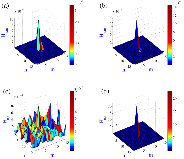
Figure 30: Energy density profiles $H_{n,m}$ plotted as a function of $n$ and $m$ at $\tau=10^{5}~{}T_{SQ}$ time units for $N_{x}=N_{y}=16$, $\lambda_{x}=\lambda_{y}=-0.02$, and $\beta_{L}=0.86$. An edge ($C$) SQUID is initially excited with amplitude (a) $A_{m}=0.001$; (b) $0.01$; (c) $0.1$; (d) $1$.

In order to roughly determine the boundaries between these three regimes, i.e., the linear, the intermediate, and the nonlinear one, the energetic participation ratio

$$P_{e}=\frac{1}{\sum_{n,m}\epsilon_{n,m}^{2}},\qquad\epsilon_{n,m}=\frac{H_{n,m}}{H}$$ (97)

is used to quantify the degree of localization of the resulting flux states. Note that $P_{e}$ measures roughly the number of excited cells in the SLiMM; its values range from $P_{e}=1$ (strong localization, all the energy in a single cell) to $P_{e}=N$, with $N=N_{x}N_{y}$ (the total energy is equally shared between the $N$ SQUIDs). In Fig. 31, the equations for the SLiMM are integrated numerically in time (for $\gamma=0$ and $\phi_{ext}=0$) with an initial single-site excitations of amplitude $A_{m,i}$; the integration time is long enough for the transients to die out, and for the system to be in the steady-state for a substantial time-interval. Then, the amplitude of oscillation of the initially excited SQUID $A_{m,c}$ is retrieved, along with the frequency $\Omega_{osc}$ of that oscillation (the oscillation of the flux through the initially excited SQUID), and the $P_{e}$ averaged over the steady-state integration time (denoted as $<P_{e}>$). The initial amplitude $A_{m,i}$ is increased in small steps and the calculations are repeated. That procedure is performed for both a $C$ type and an $A$ type SQUID.

The results shown in Fig. 31, reveal clearly how the linear, intermediate, and nonlinear regimes are separated according to the values of $A_{m,i}$ for the set of parameters used in the calculations. As it can be observed in Fig. 31(a), $A_{m,c}$ remains low for low initial amplitudes $A_{m,i}<0.15$, while for $A_{m,i}>0.15$ the calculated amplitude $A_{m,c}$ increases linearly with increasing $A_{m,i}$ ($A_{m,c}\simeq A_{m,i}$). The behavior for $A_{m,i}>0.15$ is a result of the strong localization due to nonlinearities and it does not depend on which kind of SQUID (edge or corner, $A$ or $B,C$) is initially excited. However, a closer look to the two curves for $A_{m,i}<0.15$ (inset), reveals significant differences, especially for $A_{m,i}<0.05$. Here, the calculated amplitude $A_{m,c}$ for $k=C$ follows the relation $A_{m,c}\simeq A_{m,i}/2$, indicating localization due to the flat band. This conclusion is also supported by Figs. 31(b) and 31(c). In Fig. 31(b), the energetic participation ratio averaged over the steady-state integration time $<P_{e}>$, for low values of $A_{m,i}$ attains very different values depending on which kind of SQUID is initially excited, $A$ or $C$ ($<P_{e}>\sim 140$ and $<P_{e}>\sim 10.5$, respectively). That large difference is due to delocalization in the former case and flat-band localization in the latter case. In the inset of Fig. 31(b), it can be observed that $<P_{e}>$ for an initially excited $C$ SQUID starts increasing for $A_{m,i}>0.05$ indicating gradual degradation of flat-band localization and meets the $<P_{e}>$ curve for an initially excited $A$ SQUID at $A_{m,i}\sim 0.1$. In Fig. 31(c), for $A_{m,i}<0.15$, the oscillation frequency $\Omega_{osc}$ (either of an $A$ kind or a $C$ kind SQUID) is around that of the linear resonance frequency of a single SQUID, $\Omega_{SQ}$. As it can be seen in the inset of Fig. 31(c), when a $C$ SQUID is initially excited, then $\Omega_{osc}=\Omega_{SQ}$ for $A_{m,i}\lesssim 0.075$. However, when an $A$ SQUID is initially excited, the frequency $\Omega_{osc}$ jumps slightly above and below $\Omega_{SQ}$ irregularly, but it remains within the bandwidth of the linear frequency spectrum. For $A_{m,i}>0.15$, the frequency $\Omega_{osc}$ decreases with increasing $A_{m,i}$, although it starts increasing again with increasing $A_{m,i}$ at $A_{m,i}\sim 0.8$. In this regime, nonlinear localized modes of the discrete breather type are formed, which frequency and its multitudes lie outside the linear frequency spectrum and depends on its amplitude, as it should be. Thus, for the parameter set used in these calculations, it can be inferred that flat-band localization occurs for initial amplitudes up to $A_{m,i}\simeq 0.05$ (linear regime), while delocalization occurs in the interval $0.05<A_{m,i}<0.15$ (intermediate regime). For larger $A_{m,i}$, strong nonlinear localization with $<P_{e}>\sim 1$ occurs (nonlinear regime).

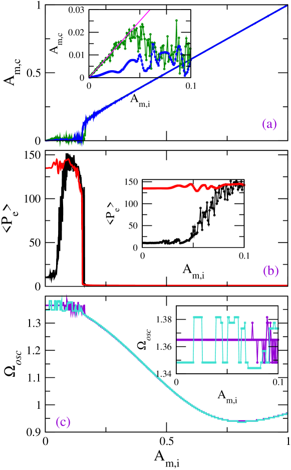
Figure 31: ( (a) The amplitude $A_{m,c}$ of the flux $\phi_{n_{e},m_{e}}^{k}$ of the initially excited SQUIDs with $k=A$ (blue curve) and $k=C$ (green curve) calculated at the end of the integration time as a function of the initial excitation amplitude $A_{m,i}$. Inset: Enlargement around low $A_{m,i}$. The line $A_{m,i}/2$ is shown in magenta color. (b) The energetic participation ratio averaged over the steady-state integration time, $<P_{e}>$, (transients were discarded) for the SQUID Lieb metamaterial when a corner ($A$) SQUID (red curve) and an edge ($C$) SQUID (black curve) is initially excited, as a function of the initial excitation amplitude $A_{m,i}$. (c) The oscillation frequency $\Omega_{osc}$ of the flux $\phi_{n_{e},m_{e}}^{k}$ of the initially excited $k=A$ (violet curve) and $k=C$ (turquoise curve) SQUID as a function of the initial excitation amplitude $A_{m,i}$. Parameters: $N_{x}=N_{y}=16$, $\lambda_{x}=\lambda_{y}=-0.02$, and $\beta_{L}=0.86$.

Remarkably, flat-band localization occurs only when an edge SQUID ($B$ or $C$) is initially excited. The excitation of a corner ($A$) SQUID does not lead to excitation of flat-band modes and thus such an initial state delocalizes rapidly. Note that the observed flat-band localization is not very strong as compared to the nonlinear localization because single-site excitations of a $B$ or $C$ SQUID do not correspond to exact localized flat-band eigenmodes.

5 Quantum Superconducting Metamaterials

5.1 Introduction

In the 1980’s, A. Leggett envisioned the possibility of achieving quantum coherence in macroscopic circuits comprising Josephson junctions; since then, the macroscopic quantum effects which are present in low-capacitance Josephson junction circuits allowed for the realization of several kinds of superconducting, effectivelly two-level quantum systems capable of storing information in binary form, i.e., superconducting quantum bits or qubits. These solid-state qubit devices are currently at the heart of quantum information processing schemes, since they seem to satisfy the requirements for being the building blocks of viable quantum computers ^{324, 325, 326}. Indeed, they found to exhibit relatively long coherence times, extremely low dissipation, and scalability ³²⁷. Several variants of superconducting qubits which relay on the Josephson effect ¹⁵⁶ and utilize either charge or flux or phase degrees of freedom have been proposed for implementing a working quantum computer; the recently anounced, commercially available quantum computer with more than $1000$ superconducting qubit CPU, known as D-Wave 2X^TM (the upgrade of D-Wave Two^TM with $512$ qubits CPU), is clearly a major advancement in this direction. A single superconducting charge qubit (SCQ) ³²⁸ at milikelvin temperatures can be regarded under certain conditions as an artificial two-level ”atom” in which two states, the ground and the first excited ones, are coherently superposed by Josephson coupling. When coupled to an electromagnetic (EM) vector potential, a single SCQ does behave, with respect to the scattering of EM waves, as an atom in space. This has been confirmed for a ”single-atom laser” consisted of a superconducting charge qubit coupled to a transmission line resonator playing the role of a ”cavity”) ³²⁹. Thus, it would be anticipated that a periodic arrangements of such qubits would demonstrate the properties of a transparent material, at least in a particular frequency band. The idea of building materials comprising artificial ”atoms” with engineered properties, i.e., metamaterials, and in particular superconducting ones, is currently under active development. Superconducting quantum metamaterials (SCQMMs) comprising a large number of qubits could hopefully maintain quantum coherence for times long enough to reveal new, exotic collective properties.

The first SCQMM which was implemented recently, comprises $20$ flux qubits arranged in a double chain geometry ¹⁵⁴. Furthermore, lasing in the microwave range has been demonstrated theoretically to be triggered in an SCQMM initialized in an easily reachable factorized state ¹⁵⁰. The considered system comprised a large number of SCQs which do not interact directly, placed in a one-dimensional (1D) superconducting waveguide. In this SCQMM, the lasing, i.e., a coherent transition of qubits to the lower-energy (ground) state was triggered by an initial field pulse traveling through the system. That type of dynamics is associated with the induced qubit-qubit coupling via their interaction with the EM field. The decoherence time of realistic SCQs as well as the relaxation times of 1D superconducting resonators and superconducting transmission lines (STLs) exceed significantly the characteristic times of energy transfer between the SCQs and the EM field, even for weak SCQ - EM field interaction. Thus, decoherence and leakage can be neglected ¹⁴⁴. The lasing dynamics of that SCQMM is also accompanied by two peculiar phenomena, i.e., the appearance of higher harmonics of the EM field and the chaotization of SCQ subsystem dynamics. The lasing process in SCQMMs has been found to be quite robust against disorder arising from unavoidable variations of the parameters of the SCQs in the fabrication process ³³⁰. That disorder makes the level-splittings of the SCQs as well as other SCQMM parameters to vary locally in a random way. For the investigation of that process, a model Tavis-Cummings Hamiltonian was employed, which holds not only for real atoms but also for artificial ones, such as superconducting flux and charge qubits. Disordered SCQMMs comprising superconducting flux qubits with randomly varying excitation frequencies in a microwave resonator have been also investigated with a model Tavis-Cummings Hamiltonian which contained a qubit-qubit interaction term ³³¹. It is demonstrated that photon phase-shift measurements allow to distinguish individual resonances in that flux qubit metamaterial with up to a hundred qubits. Numerical simulations of the phase-shift as a function of external flux (which modifies the qubit excitation energies), using exact diagonalization of the Hamiltonian in a single excitation basis, are in agreement with recent experimental results ¹⁵⁴. Further theoretical studies have revealed the emergence of collective quantum coherent phenomena using an approach borrowed from mesoscopic physics ¹⁴⁹. It is demonstrated that the chain of $N$ qubits, incorporated into a low-dissipation resonant cavity, exhibits synchronized dynamics, even though the energy splittings $\Delta_{i}$ and thus the excitation frequencies $\omega_{i}=\Delta_{i}/\hbar$ are different from one qubit to the other. Those quantum coherent oscillations are characterized by two frequencies, $\omega_{1}=\bar{\Delta}/\hbar$ and $\omega_{2}=\tilde{\omega}_{R}$ where $\bar{\Delta}=(1/N)\sum_{i=1}^{N}\Delta_{i}$ with $\tilde{\omega}_{R}$ being the resonator frequency ”dressed” by the interaction. In a similar SCQMM, i.e., a charge qubit array embedded in a low-dissipative resonator, various equilibrium photon states were investigated ³³². When the photon energy of the resonator $\hbar\omega_{0}$ is much smaller than the energy splitting of qubits $\Delta$ (identical qubits have been considered), a second order phase transition is obtained in the state of photons. Specifically, at $T>T^{\star}$ (high temperatures, with $T^{\star}$ being the transition temperature) the photon state is incoherent. At $T<T^{\star}$ (low temperatures), however, coherent states of photons with two different polarizations occur in such a SCQMM. Interestingly, these two macroscopic coherent states of photons have equal energies, but they are separated by a barrier. Different photon states manifest themselves as resonant drops in the frequency-dependent transmission coefficient $D(\omega)$; thus, incoherent and coherent photon states display a single drop and three drops, respectively, in their $D(\omega)$. Moreover, the resonant structure of $D(\omega)$ in the latter case provides direct evidence of macroscopic quantum oscillations between two different coherent states of photons. Quantum synchronization has been also demonstrated theoretically for a disordered SCQMM (in which the energy splitting of the $i-$th qubit is $\Delta_{i}$) comprising an array of flux qubits (3-Josephson junction SQUIDs) which is coupled to a transmission line ³³³.

Also, remarkable quantum coherent optical phenomena, such as self-induced transparency ³³⁴ (SIT) and Dicke-type superradiance ³³⁵ (collective spontaneous emission, SRD), occur during light-pulse propagation in SCQMMs comprising SCQs ¹⁵¹. The occurence of the former or the latter effect solely depends on the initial state of the SCQ subsystem. Specifically, in self-induced transparency (superradiance) all the SCQs are initially in their ground (excited) state; such an extended system exhibiting SIT or SRD effects is often called a coherent amplifier or attenuator, respectively. These fundamental quantum coherent prosesses have been investigated extensively in connection to one- and two-photon resonant two-level systems. It is demonstrated that SIT or SRD electomagnetic pulses propagating in the SCQMM induce to that quantum coherence in the form of ”population inversion” pulses, which move together with the SIT or SRD EM pulses at the same speed. The experimental confirmation of such quantum coherence effects in SCQMMs may open a new pathway to potentially powerful quantum computing. Superradiant effects have been recently observed in quantum dot arrays ³³⁶ and spin-orbit coupled Bose-Einstein condensates ³³⁷. These findings suggest that these systems can radiatively interact over long distances.

5.2 Superconducting Qubits

In the past twenty years, impressive progress has been achieved both experimentally and theoretically in superconducting quantum bits (qubits), which comprise Josephson junctions. Those superconducting qubits have opened a new research area with many potential applications in quantum-information processing. The Josephson junctions ¹⁵⁶, which are equivalent to nonlinear inductors, provide strong nonlinearity to the superconducting qubits; this is a desired property for designing effectively two-level systems, as we discuss below. The superconducting qubits are essentially macro-mesoscopic devices which enter into the fully quantum regime at milli-Kelvin temperatures; such low temperatures are needed for the superconducting qubits to maintain their quantum states. In close analogy to natural atoms, the superconducting qubits have discrete energy levels and therefore can be regarded as artificial atoms. In contrast to natural atoms, however, their properties (e.g., their energy levels) as well as the coupling between them can be engineered and/or adjusted by external fields. Here, we briefly present the basics for superconducting qubits. A basic requirement for the superconducting qubits to function as artificial two-level systems (i.e., bits) is the nonlinearity, which differentiates the energy spacing between sequencial energy levels. As far as that spacing is concerned, the Josephson junctions play an important role as highly nonlinear elements. Moreover, Josephson junctions have negligibly small energy dissipation, which is yet another desired property for a superconducting qubit component. From the two celebrated Josephon relations discussed in Section $2.1$ (Eq. (1)) it can be easily deduced that an ideal Josephson juction acts as a nonlinear inductance

$$L_{J}=\frac{\hbar}{2eI_{c}\cos\phi_{J}},$$ (98)

whose value may even become negative. In Eq. (98), $\hbar$ is the Planck’s constant devided by $2\pi$, $e$ is the eletron’s charge, $I_{c}$ is the critical current which characterizes the Josephson junction, and $\phi_{J}$ is the gauge-invariant Josephon phase which has been discussed in Subsection $2.1$.

In an electrical equivalent circuit consideration of superconducting qubits, it is exactly that equivalent Josephson inductance $L_{J}$ that provides the desired nonlinearity. Thus, in a given superconducting qubit, the two lowest energy levels can be selected to form an effectively two-level system (a bit), appropriate for quantum information processing. There are three basic types of superconducting qubits comprising Josephson junctions, which are usually operating at frequencies in the microwave regime, which rely on different ”degrees of freedom”, i.e., either on charge, or flux, or phase. They are classified by the ratio of the Josephson energy to the charging (capacitive) energy

$$\varepsilon_{q}=\frac{E_{J}}{E_{C}},~{}~{}~{}{\rm where}~{}~{}~{}E_{J}=\frac{\hbar I_{c}}{2e},~{}~{}~{}E_{C}=\frac{e^{2}}{2C_{J}}.$$ (99)

In Eq. (99), $E_{J}$ and $E_{C}$ denote the Josephson and charging energy, respectively, $C_{J}$ denotes the capacitance of the Josephson junction. The quantized superconducting qubits are described by the canonically conjugate variables $\phi_{J}$, i.e., the gauge-invariant Josephson phase, and the number of Cooper pairs $n$. Those variables satisfy the commutation relation $[\phi_{J},n]=i$ and obey the Heisenberg uncertainty principle $\Delta\phi_{J}\Delta n\geq 1$. It is important to note that the operator $n$ has integer eigenvalues whereas $\phi_{J}$ is an operator corresponding to the position of a point on the unit circle (an angle modulo $2\pi$). For large enough systems with $n>>1$, the number operator $n$ can be replaced by $-i\partial/\partial\phi_{J}$. The three basic types of superconducting qubits, i.e., phase, flux, and charge qubits are distinguished by the relations between the parameters $E_{C}$, $E_{J}$, and the energy difference between the two levels $\hbar\omega_{0}$, with $\omega_{0}=\sqrt{2E_{C}E_{J}}/\hbar$. The three basic types of qubits have been described in great detail in several excellent review articles ^{338, 339, 340, 327, 341}. Therefore, here we only briefly refer to them.

Charge qubits. The prototypical charge qubit (also called Cooper pair box) was the first to be described theoretically. Superconducting charge qubits (SCQs) are usually formed by small superconducting islands with $n$ Cooper pairs grounded through a Josephson junction. A gate voltage $V_{g}$ can be applied to that island through a (gate) capacitance $C_{g}$, in order to control the spacing between the energy-levels of the SCQ. Then, for a non-zero $V_{g}$, the charging energy is $E_{C}=\frac{e^{2}}{2(C_{J}+C_{g})}$, with $C_{J}$ being the capacitance of the Josephson junction, and $n_{g}=C_{g}V_{g}/(2e)$ is the gate-charge number. It can be shown that the Hamiltonian of that device is

$$H=E_{C}\left(n-n_{g}\right)^{2}-E_{J}\cos(\phi_{J}).$$ (100)

The eigenenergies and eigenfunctions of the Hamiltonian Eq. (100) can be calculated in terms of special functions which are known with arbitrary precision. Note that the eigenspectrum can be modified either by varying $n_{g}$ or $E_{J}$. Let us now limit ourselves to the two lowest levels of the box. Then, near the degeneracy point (optimal point) $n_{g}=1/2$, where the two charge states $|n=0>$ and $|n=1>$ (which differ by a single Cooper pair) have equal electrostatic energy, the Hamiltonian Eq. (100) can be reduced to

$$H_{q}=-E_{z}\left(\sigma_{z}+X_{c}\sigma_{x}\right),$$ (101)

where $\sigma_{x}$ and $\sigma_{z}$ are the Pauli spin operators. The eigenstates of Hamiltonian (101) are coherent superpositions of the states $|n=0>$ and $|n=1>$, i.e., they are of the form $(|n=0>\pm|n=1>)/\sqrt{2}$. In the limit $E_{C}>>E_{J}$, in which the charging behavior of the capacitance dominates, we have that $E_{z}=E_{J}/2$ and $X_{c}=2(E_{C}/E_{J})[(1/2)−n_{g}]$. The main disadvantage of the charge qubit is its very strong sensitivity to charge noise, which can be mitigated to some extent by operating the qubit in the intermediate regime $E_{J}\lesssim E_{C}$.

Phase qubits.- Phase qubits operate in the ”phase regime” in which the Josephson term dominates the Hamiltonian (100), i.e., when $E_{C}\lesssim E_{J}$. They consist of a single Josephson junction which is biased by an external current $I_{b}$. The Hamiltonian of the superconducting phase qubit can be written as

$$H=-E_{C}\partial_{\phi_{J}}^{2}-E_{J}\cos(\phi_{J})-\frac{I_{b}\Phi_{0}}{2\pi}\phi_{J}\equiv-E_{C}\partial_{\phi_{J}}^{2}-E_{J}\left(\cos(\phi_{J})+\frac{I_{b}}{I_{c}}\right),$$ (102)

which is the Hamiltonian of a quantum particle in a tilted washboard potential. The phase qubit operates typically in the subcritical regime (in practice, when $I_{b}\simeq 0.95I_{c}-0.98I_{c}$), so that only a few quantized levels remain in each local minimum of the Josephson potential $U_{J}=-E_{J}\left(\cos(\phi_{J})+\frac{I_{c}}{I_{b}}\right)$. The tunneling probability out of the lowest two levels is very small, and thus these can be taken as qubit states $|0>$ and $|1>$. For $I_{b}\simeq I_{c}$ we have that $\phi_{J}\simeq\pi/2$ and the Josephson potential can be approximated by

$$U_{J}=E_{J}\left[\left(1-\frac{I_{c}}{I_{b}}\right)\phi_{J}-\frac{1}{6}\phi_{J}^{3}\right].$$ (103)

The classical oscillation frequency at the bottom of the well (so-called plasma oscillation) is given by

$$\omega_{p}=\omega_{0}\left[\left(1-\frac{I_{b}}{I_{c}}\right)^{2}\right]^{1/4}.$$ (104)

Quantum-mechanically, energy levels can be found for the potential in Eq. (103 with non-degenerate spacings. The first two levels, which have a transition frequency $\omega_{01}\simeq 0.95\omega_{p}$, can be used for qubit states. In practive, $\omega_{01}/(2\pi)$ falls in the $5-20~{}GHz$ range. Defining $\Delta I\equiv I_{b}-Ic$, the phase qubit Hamiltonian is given by

$$H_{q}=\frac{\hbar\omega_{01}}{2}\sigma_{z}+\sqrt{\frac{\hbar}{2\omega_{01}C}}\Delta I\left(\sigma_{x}+\chi\sigma_{z}\right),$$ (105)

where $\chi=\sqrt{\frac{\hbar\omega_{01}}{3\Delta U}}\simeq 1/4$ for typical operating parameters, with $\Delta U=\frac{2\sqrt{2}}{3}I_{c}\left(1-\frac{I_{c}}{I_{b}}\right)^{3/2}$.

Flux qubits.- Another possibility to realize a qubit in the limit $E_{J}>>E_{C}$ is to take advantage of the degeneracy between two current-carrying states of an rf SQUID. The Hamiltonian for this system can be written as

$$H=-E_{C}\partial_{\phi_{J}}^{2}-E_{J}\cos(\phi_{J})+\frac{1}{2}E_{L}\left(\phi_{J}-\phi_{ext}\right)^{2},$$ (106)

where $\phi_{ext}=2\pi\frac{\Phi_{ext}}{\Phi_{0}}$ is the reduced flux through the loop of the rf SQUID due to an external magnetic field, and $E_{L}=\frac{\Phi_{0}^{2}}{2\pi L}$ is the inductive energy due to the self-inductance $L$ of the rf SQUID. The potential energy is in this case formed by the last two terms in the Hamiltonian Eq. (106). For $\phi_{ext}\simeq\pi$, the potential of the rf SQUID has two almost degenerate minimums. The lowest energy states correspond to a persistent current circulating in the loop of the rf SQUID in opposite directions, and they can be conveniently used as the the $|0>$ and $|1>$ states of the flux qubit. Tunneling between the two potential wells is enabled by the first term in Eq. (106). Then, in the $\{|0>,|1>\}$ subspace, the effective flux qubit Hamiltonian is

$$H=-\frac{\varepsilon}{2}\sigma_{z}+\frac{\Delta}{2}\sigma_{x},$$ (107)

where $\varepsilon\propto<1|H_{q}|1>-<0|H_{q}|0>$ is the energy bias between the two levels (level splitting or ”gap”), and $\Delta\propto<0|H_{q}|1>$ is the tunneling amplitude. For $\phi_{ext}=\pi$, i.e., exactly on the degeneracy point, we have that $\varepsilon=0$ and the eigenstates of the Hamiltonian Eq. (107) are again of the form $\left(|0>\pm|1>\right)/\sqrt{2}$.

5.3 Self-Induced Transparency, Superradiance, and Induced Quantum Coherence

5.3.1 Description of the Model System

Consider an infinite, one-dimensional (1D) periodic array comprising Superconducting Charge Qubits (SCQs). That array is placed in a Superconducting Transmission Line (STL) consisting of two superconducting strips of infinite length ^{144, 148}, as shown in Fig. 32(a); each of the SCQs, in the form of a tiny superconducting island, is connected to each bank of the STL by a Josephson junction (JJ). Control circuitry can be added to that structure, so that each individual SCQ is coupled to a gate voltage source $V_{g}$ through a gate capacitor $C_{g}$ (Fig. 32(c). Thus, local control of the SCQMM can be achieved by altering independently the state of each SCQ ¹⁴². The SCQs exploit the nonlinearity of the Josephson effect ¹⁵⁶ and the large charging energy resulting from nanofabrication to create artificial mesoscopic two-level systems. A propagating EM field in the STL gives rise to indirect interactions between the SCQs, which are mediated by its photons ³⁴². Those interactions are of fundamental importance in quantum optics, quantum simulations, and quantum information processing, as well. Since the qubits can be in a coherent superposition of quantum states, such a system demonstrates interesting effects, e.g., it may behave as a ”breathing” photonic crystal with an oscillating band gap ¹⁴⁴. That gap depends on the quantum state of the qubits, that makes this system a quantum photonic crystal. Thus, a variation of the microscopic quantum state of the qubits will change the macroscopic EM response of the system. The key ingredient of these effects is that the optical properties of the Josephson transmission line are controlled by the quantum coherent state of the qubits. The progress on the emerging field of microwave photonics with superconducting quantum circuits has been reviewed in Ref. ³⁴³. Below we discuss two remarkable quantum coherent optical phenomena, i.e., self-induced transparency and Dicke-type superradiance, which may occur during light-pulse propagation in the above mentioned SCQMM. Moreover, it appears that the propagating pulses induce quantum coherence in the chain of SCQs, in the form of ”population inversion” pulses.

In the following, the essential building blocks of the SCQMM model are summarized in a self-contained manner, yet omitting unnecessary calculational details which are presented in the Appendix. The system of units in Refs. ^{144, 148} is used from here to the end of the article. An EM vector potential pulse $\vec{A}=A_{z}(x,t)\hat{z}$ can propagate in the SCQMM structure, which extends over the $x-$direction, and couples to the SCQs. Then, the energy per unit cell of the SCQMM - EM vector potential pulse can be readily written in units of the Josephson energy $E_{J}=\frac{\Phi_{0}I_{c}}{2\pi C}$, with $\Phi_{0}$, $I_{c}$ and $C$ being the magnetic flux quantum, the critical current of the JJ, and the capacitance of the JJ, respectively, as ^{144, 148}

$$H=\sum_{n}\left\{\left[\dot{\varphi}^{2}_{n}-2\cos\varphi_{n}\right]+\left[\dot{\alpha}^{2}_{n}+\beta^{2}(\alpha_{n+1}-\alpha_{n})^{2}\right]+\left[2\cos\varphi_{n}(1-\cos\alpha_{n})\right]\right\},$$ (108)

where $\varphi_{n}$ is the superconducting phase on the $n$th island, $\alpha_{n}=2\pi dA_{x,n}/\Phi_{0}$ is the normalized and discretized EM vector potential in the center of the $n$th unit cell, with $d$ being the separation between the electrodes of the STL, $\beta=\frac{1}{\sqrt{8\pi ldE_{J}}}\frac{\Phi_{0}}{2\pi}$, and the overdots denote differentiation with respect to the temporal variable $t$. The three terms in the square brackets in Eq. (108) represent the energy of the SCQs (equivalently the energy of the two JJs in an EM vector potential having the orientation shown in Fig. 32(b)), the energy of the EM field, and their interaction energy, respectively.

For the discretization of the EM vector potential, it is assumed that the wavelength $\lambda$ of the carrier EM field with vector potential $A_{z}(x,t)$ is much larger that all the other characteristic lengths of the SCQMM structure, i.e., that $\lambda>>\ell,d$, with $\ell$ being the distance between neighboring SCQs. Then, the EM potential can be regarded to be approximately constant within a unit cell, so that in the center of the $n$th unit cell $A_{z}(x,t)\simeq A_{z,n}(t)$ or equivalently $\alpha(x,t)\simeq\alpha_{n}(t)$. Note that the coupling between the SCQs and the EM field is realized from the requirement of having gauge-invariant Josephson phase in each of the junctions.

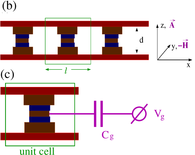
Figure 32: Schematic drawing of a superconducting quantum metamaterial comprising charge qubits. (a) An infinite chain of identical charge qubits periodically loaded in a superconducting transmission line (STL). Each qubit is a tiny superconducting island that is connected to the electrodes of the STL through two Josephson junctions, formed in the regions of the insulating (dielectric) layers (blue). The propagating electromagnetic vector potential pulse is also shown schematically and out of scale. (b) Side view of the SCQMM in which the relevant geometrical parameters and the field orientations are indicated. (c) A single unit cell of the SCQMM, in which the control circuitry for each individual charge qubit is shown. The gate potential $V_{g}$ is applied to a superconducting charge qubit through the gate capacitor $C_{g}$.

5.3.2 Second Quantization and Reduction to Maxwell-Bloch Equations

The quantization of the SCQ subsystem requires the replacement of the classical variables $\varphi_{n}$ and $\dot{\varphi}_{n}$ by the corresponding quantum operators $\hat{\varphi}_{n}$ and $-i({\partial}/{\partial\hat{\varphi}_{n}})$, respectively. While the EM field is treated classically, the SCQs are regarded as two-level systems, so that only the two lowest energy states are retained; under these considerations, the second-quantized Hamiltonian corresponding to Eq. (108) in the semi-classical approximation is

$$H=\sum_{n}\sum_{p}E_{p}(n)a^{\dagger}_{n,p}a_{n,p}+\sum_{n}\left[\dot{\alpha}^{2}_{n}+\beta^{2}(\alpha_{n+1}-\alpha_{n})^{2}\right]+4\sum_{n}\sum_{p,p^{\prime}}V_{p,p^{\prime}}(n)a^{\dagger}_{n,p}a_{n,p^{\prime}}\sin^{2}\frac{\alpha_{n}}{2},$$ (109)

where $p,p^{\prime}=0,1$, $E_{0}$ and $E_{1}$ are the energy eigenvalues of the ground and the excited state, respectively, the operator $a^{\dagger}_{n,p}$ ($a_{n,p}$) excites (de-excites) the $n$th SCQ from the ground to the excited (from the excited to the ground) state, and $V_{p,p^{\prime}}=\int d\varphi\Xi^{*}_{p}(\varphi)\cos\varphi\Xi_{p}(\varphi)$ are the matrix elements of the effective SCQ - EM field interaction. The basis states $\Xi_{p}$ can be obtained by solving the single-SCQ Schrödinger equation $(-{\partial^{2}}/{\partial\varphi^{2}}-E_{p}+2\cos\varphi)\Xi_{p}=0$. In general, each SCQ is in a superposition state of the form $|\Psi_{n}\rangle=\sum_{p}\Psi_{n,p}(t)a^{\dagger}_{n,p}|0\rangle$. The substitution of $|\Psi_{n}\rangle$ into the Schrödinger equation with the second-quantized Hamiltonian Eq. (109), and the introduction of the Bloch variables

$$R_{x}(n)=\Psi^{\star}_{n,1}\Psi_{n,0}+\Psi^{\star}_{n,0}\Psi_{n,1},\qquad R_{y}(n)=i(\Psi^{\star}_{n,0}\Psi_{n,1}-\Psi^{\star}_{n,1}\Psi_{n,0}),\qquad R_{z}(n)=|\Psi_{n,1}|^{2}-|\Psi_{n,0}|^{2},$$ (110)

provides the re-formulation of the problem into the Maxwell-Bloch equations

$$\dot{R}_{x}(n)=-\left[\Delta+8D\sin^{2}\frac{\alpha_{n}}{2}\right]R_{y}(n),~{}\dot{R}_{y}(n)=\left[\Delta+8D\sin^{2}\frac{\alpha_{n}}{2}\right]R_{x}(n)-8\mu\sin^{2}\frac{\alpha_{n}}{2}R_{z}(n),~{}\dot{R}_{z}(n)=+8\mu\sin^{2}\frac{\alpha_{n}}{2}R_{y}(n),$$ (111)

that are nonlinearly coupled to the resulting equation for the normalized EM vector potential

$$\ddot{\alpha}_{n}+\left\{\Omega^{2}+\chi\left[\mu R_{x}(n)+DR_{z}(n)\right]\right\}\sin\alpha_{n}=\beta^{2}\delta a_{n},$$ (112)

where

$$\delta\alpha_{n}=\alpha_{n-1}-2\alpha_{n}+\alpha_{n+1},~{}~{}D=\frac{(V_{11}-V_{00})}{2\chi},~{}~{}\Omega^{2}=\frac{(V_{00}+V_{11})}{2},~{}~{}\mu=\frac{V_{10}}{\chi}=\frac{V_{01}}{\chi},~{}~{}\Delta=\epsilon_{1}-\epsilon_{0}\equiv\frac{(E_{1}-E_{0})}{\chi},$$ (113)

with $\chi=\hbar\frac{\omega_{J}}{E_{J}}$. In Eqs. (111) and (112), the overdots denote differentiation with respect to the normalized time $t\rightarrow\omega_{J}t$, in which $\omega_{J}=\frac{eI_{c}}{\hbar C}$ is the Josephson frequency and $e$, $\hbar$ are the electron charge and the Planck’s constant devided by $2\pi$, respectively.

5.3.3 Approximations and Analytical Solutions

For weak EM fields, $|\alpha_{n}|\ll 1$ for any $n$, the sine term can be linearized as $\sin\alpha_{n}\simeq\alpha_{n}$. Then, by taking the continuum limit of Eqs. (111) and (112), using the relations $\alpha_{n}(t)\rightarrow\alpha(x,t)$ and $R_{i}(n;t)\rightarrow R_{i}(x;t)$ $(i=x,y,z)$, a set of simplified, yet still nonlinearly coupled equations is obtained, similar to those encountered in two-photon self-induced transparency (SIT) in resonant media ³⁴⁴. Further simplification can be achieved with the slowly varying envelope approximation (SVEA), using the ansatz $\alpha(x,t)=\varepsilon(x,t)\cos\Psi(x,t)$ for the EM vector potential, where $\Psi(x,t)=kx-\omega t+\phi(x,t)$ and $\varepsilon(x,t)$, $\phi(x,t)$ are the slowly varying pulse envelope and phase, respectively, with $\omega$ and $k$ being the frequency of the carrier wave of the EM pulse and its wavenumber in the STL, respectively. The dispersion relation (see the Appendix for the derivation)

$$k=\pm\frac{\sqrt{\omega^{2}-\Omega^{2}}}{\beta},$$ (114)

provides the dependence of $k$ on $\omega$ or vice versa. In the absence of the SCQ chain, the EM pulse propagates in the STL with speed $\beta$. At the same time, Eqs. (111) for the Bloch vector components are transformed according to

$$R_{x}=r_{x}\cos(2\Psi)+r_{y}\sin(2\Psi),\qquad R_{y}=r_{y}\cos(2\Psi)-r_{x}\sin(2\Psi),\qquad R_{z}=r_{z}.$$ (115)

Then, collecting the coefficients of $\sin\Psi$ and $\cos\Psi$ while neglecting the rapidly varying terms, and averaging over the phase $\Psi$, results in a set of truncated equations. Further manipulation of the resulting equations and the enforcement of the two-photon resonance condition $\Delta=2\omega$, results in

$$\dot{\varepsilon}+c\varepsilon_{x}=-\chi\frac{\mu}{\Delta}\varepsilon r_{y},\qquad\dot{\phi}+c\phi_{x}=-\chi\frac{2D}{\Delta}r_{z},$$ (116)

where $c=\frac{\beta^{2}k}{\omega}=2\frac{\beta^{2}k}{\Delta}$, and the truncated Maxwell-Bloch equations

$$\dot{r}_{x}=-2D\varepsilon^{2}r_{y},\qquad\dot{r}_{y}=+2D\varepsilon^{2}r_{x}-\frac{\mu\varepsilon^{2}}{2}R_{z},\qquad\dot{r}_{z}=+\frac{\mu\varepsilon^{2}}{2}r_{y},$$ (117)

in which the $n-$dependence of the $r_{i}$ $(i=x,y,z)$ is suppressed, in accordance with common practices in quantum optics. Also, from Eqs. (117), the conservation law $r_{x}^{2}+r_{y}^{2}+r_{z}^{2}=1$ can be obtained.

The $r_{i}$ can be written in terms of new Bloch vector components $S_{i}$ using the unitary transformation

$$r_{x}=S_{x}\cos\Phi-S_{z}\sin\Phi,\qquad r_{y}=S_{y},\qquad r_{z}=S_{z}\cos\Phi+S_{x}\sin\Phi,$$ (118)

where $\Phi$ is a constant angle which will be determined later. Using a procedure similar to that for obtaining the $r_{i}$, we get

$$\dot{S}_{x}=0,\qquad\dot{S}_{y}=-\frac{1}{2}W\varepsilon^{2}S_{z},\qquad\dot{S}_{z}=+\frac{1}{2}W\varepsilon^{2}S_{y},$$ (119)

where $W=\sqrt{(4D)^{2}+\mu^{2}}$ and $\tan\Phi\equiv\gamma=\frac{4D}{\mu}$. The combined system of Eqs. (119) and (116) admits exact solutions of the form $\varepsilon=\varepsilon(\tau=t-x/v)$ and $S_{i}=S_{i}(\tau=t-x/v)$, where $v$ is the pulse speed. For the slowly varying pulse envelop, we obtain

$$\varepsilon(\tau)=\varepsilon_{0}\left[1+\left(\frac{\tau-\tau_{0}}{\tau_{p}}\right)^{2}\right]^{-\frac{1}{2}},$$ (120)

where the pulse amplitude an its duration are given respectively by

$$\varepsilon_{0}=\sqrt{\frac{8\sigma^{2}}{\Delta}\frac{v}{(c-v)}},\qquad\tau_{p}=\left\{2\chi\frac{\sigma\mu}{\Delta}\frac{v}{(c-v)}\right\}^{-1},$$ (121)

with $\sigma=\frac{\mu}{W}=\frac{1}{\sqrt{1+\gamma^{2}}}$. The decoherence factor $\gamma$ can be expressed as a function of the matrix elements of the effective interaction between the SCQ subsystem and the EM field, $V_{ij}$, as $\gamma=2\frac{(V_{11}-V_{00})}{V_{10}}$ that can be calculated when the latter are known. Lorentzian propagating pulses of the form of Eq. (120) have been obtained before in two-photon resonant media ^{345, 346}; however, SIT in quantum systems has only been demonstrated in one-photon (absorbing) frequency gap media, in which solitonic pulses can propagate without dissipation ³⁴⁷. The corresponding solution for the population inversion, $R_{z}$, reads

$$R_{z}(\tau)=\pm\left[-1+\left(\frac{\varepsilon(\tau)}{\varepsilon_{M}}\right)^{2}\right],$$ (122)

where $\varepsilon_{M}=\sqrt{\frac{8}{\Delta}\frac{v}{(c-v)}}$, and the plus (minus) sign corresponds to absorbing (amplifying) SCQMMs; these are specified through the initial conditions as

$$R_{x}(-\infty)=R_{y}(-\infty)=0,\qquad R_{z}(-\infty)=-1,\qquad\varepsilon(-\infty)=0,$$ (123)

for absorbing SCQMMs, and

$$R_{x}(-\infty)=R_{y}(-\infty)=0,\qquad R_{z}(-\infty)=+1,\qquad\varepsilon(-\infty)=0,$$ (124)

for amplifying SCQMMs. The initial conditions specified by Eqs. (123) (Eqs. (124)) ensure that before the arrival of the EM pulse, all the SCQs are in their ground (excited) state in order to achieve absorption (amplification). Since the frequency $\omega$ has been chosen to match the two-photon resonance, the wavevector $k$ has been uniquely determined through the dispersion relation Eq. (114) to be $k=\pm\frac{\sqrt{\Delta^{2}-4\Omega^{2}}}{2\beta}$, or, after replacements of $\Omega$ and $\Delta$ from Eq. (113),

$$k=k_{r}=\pm\frac{\sqrt{\left(\frac{E_{1}-E_{0}}{\chi}\right)^{2}-4\frac{V_{00}+V_{11}}{2}}}{2\beta}$$ (125)

Obviously, the propagation of EM pulses in the SCQMM is only possible for real $k$. The requirement for the wavenumber $k$ to be real results in the relation

$$2\chi^{2}(V_{11}+V_{00})<(E_{1}-E_{0})^{2},$$ (126)

which provides a necessary condition for pulse propagation in the SCQMM. Note that the propagation condition Eq. (126) contains only qubit-related parameters, i.e., the diagonal matrix elements $V_{00}$, $V_{11}$ and the energy levels $E_{0}$ and $E_{1}$, whose values can be in principle tailored during fabrication or tuned in real time by the gate voltages $V_{g}$.

The corresponding velocity-amplitude relation of a propagating pulse in the SCQMM under the two-photon resonance condition reads

$$v=c\left[1\pm{\chi\frac{8\sigma^{2}}{\Delta\varepsilon_{0}^{2}}}\right]^{-1},$$ (127)

where the value of $c$ is that at the two-photon resonance $\omega=\Delta/2$, i.e., $c=c_{r}=2\beta^{2}k_{r}/\Delta$. A relation between the pulse amplitude and its duration can be obtained by combining Eqs. (121); the resulting relation is then $\varepsilon_{0}^{2}\tau_{p}=4/(\chi W)$, which can be used to transform Eq. (127) into a velocity-duration expression. From Eq. (127), it is obvious that $c_{r}=2\beta^{2}k_{r}/\Delta$ plays the role of a limiting velocity, since $v\rightarrow c$ for $\varepsilon_{0}\rightarrow\infty$. Thus, the velocity $c_{r}$ sets an upper (lower) bound on the pulse velocity in absorbing (amplifying) SCQMM structures. It is generally lower than the corresponding one for two-photon SIT or SRD in ordinary media, $\beta$. Moreover, $c_{r}$ depends only on the qubit parameters, so that its value can be also tailored during fabrication or tuned by the gate voltages $V_{g}$.

In Fig. 33, several velocity-amplitude curves $v/\beta$ as a function of $\varepsilon_{0}$ are shown along with profiles of the envelops of the EM vector potential pulse $(\varepsilon/\varepsilon_{M})^{2}$ and the population inversion $R_{z}(n)$ as functions of the slow variable $(\tau/\tau_{M})$, $\tau_{M}=\frac{\Delta}{2\chi\mu}\frac{c-v}{v}$, in a frame of reference which is moving with velocity $v$, both for absorbing and amplifying SCQMMs. In all subfigures, the horizontal magenta-solid lines indicate the limiting velocity in ordinary amplifying and absorbing mediums, $v=\beta$, while the black-solid lines indicate the limiting velocity in amplifying and absorbing SCQMMs, $v=c_{r}<\beta$. All the curves exhibit a hyperbolic dependence; moreover, the corresponding curves for ordinary mediums and SCQMMs are close to each other, especially for low $\varepsilon_{0}$. The major difference is that the limiting velocity in SCQMMs is always lower than the corresponding one in ordinary mediums. Moreover, that limiting velocity in SCQMMs is parameter-dependent as mentioned above; this becomes clear by comparing curves of the same color (e.g., the red-dashed curves) in Figs. 33a and c, for which the ratio $\Omega/\Delta$ is $0.15$ and $0.26$, respectivelly, and provides $v/\beta\simeq 0.95$ and $\simeq 0.88$. The limiting velocity $c_{r}$ for SCQMMs can be reduced further with increasing further the ratio $\Omega/\Delta$. Thus, parameter engineering for the SCQMM can slow down the speed of the pulses $v$ at the desired level for high enough amplitudes $\varepsilon_{0}$. Effective control of $v$ in SCQMMs could also be achieved in principle by an external field ³⁴⁸ or by real time tuning of the qubit parameters through the gate voltages $V_{g}$, as mentioned above. That ability to control the flow of ”optical”, in the broad sense, information may have technological relevance to quantum computing ³⁴⁹. The effect of non-zero $\gamma$ factor become apparent by comparing again curves of the same color in Figs. 33a and b, for which $\gamma=0$ and $2$, respectively (the rest of the parameters are the same). The velocity-amplitude curves approach their limiting value for lower $\varepsilon_{0}$ with increasing $\gamma$. The same conclusion can be drawn by comparing curves of the same color in Figs. 33c and d. The effect of non-zero $\gamma$ is also revealed in the insets of Figs. 33a and b; in each inset, the left (right) panel is for absorbing (amplifying) SCQMMs. In both cases, the amplitudes of the pulse envelops for $\gamma=2$ are about four times smaller than those for $\gamma=0$. Thus, only for $\gamma=0$, i.e., for $V_{00}=V_{11}$, can the envelops of the EM vector potential pulses and the population inversion pulses (either for absorbing or for amplifying SCQMMs) attain their maximum amplitude value.

Note that we have not been concerned with decoherence effects due to dephasing and energy relaxation in the SCQs. This is clearly an idealization which is partly justified as long as the coherence time exceeds the wave propagation time across a relatively large number of unit cell periods (i.e., a large number of SCQs). In a recent experiment ³⁵⁰, a charge qubit coupled to a strip line had a dephasing time in excess of $200~{}ns$, i.e., a dephasing rate of $5~{}MHz$, and a photon loss rate from the cavity of $0.57~{}MHz$. Those frequencies are very small compared with the transition frequency of the considered SCQs which is of the order of the Josephson energy (i.e., a few $GHz$) ^{144, 148}. Therefore, we have neglected such decoherence effects here. The decoherence factor $\gamma$, which in Figs. 33b and d has been chosen according to the parameter values in ¹⁴⁴, is not related to either dephasing or energy relaxation. That factor attains a non-zero value whenever the matrix elements of the effective SCQ-EM field interaction, $V_{11}$ and $V_{00}$, are not equal.

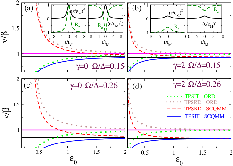
Figure 33: The normalized pulse velocity $v/\beta$ - amplitude $\varepsilon_{0}$ relation in two-photon superradiant (TPSRD, amplifying) and two-photon self-induced transparent (TPSIT, absorbing) superconducting quantum metamaterials (SCQMMs) and pulse envelops. In (a)-(d), the normalized pulse velocity $v/\beta$ is plotted as a function of the electromagnetic (EM) vector potential pulse amplitude $\varepsilon_{0}$ and compared with the corresponding curves for ordinary amplifying (brown-dotted curves) and absorbing (green-dotted curves) mediums. The horizontal magenta-solid (resp. black-solid) lines indicate the limiting velocity in ordinary amplifying and absorbing mediums, $v/\beta=1$ (resp. amplifying and absorbing SCQMMs, $v=c_{r}<\beta$). (a) $V_{00}=V_{11}=1$, $V_{01}=V_{10}=0.8$, $\chi=1/5$, $E_{1}-E_{0}=3$ ($\gamma=0$ and $\Omega/\Delta=0.15$). Left Inset: The envelop of the EM vector potential pulse $(\varepsilon/\varepsilon_{M})^{2}$ and the population inversion $R_{z}(n)$ profiles as a function of $\tau/\tau_{M}$ for TPSIT (absorbing) SCQMMs. Right Inset: Same as in the left inset for TPSRD (amplifying) SCQMMs. (b) $V_{00}=0.6$, $V_{11}=1.4$, $V_{01}=V_{10}=0.8$, $\chi=1/5$, $E_{1}-E_{0}=3$ ($\gamma=2$ and $\Omega/\Delta=0.15$). Left Inset: The envelop of the EM vector potential pulse $(\varepsilon/\varepsilon_{M})^{2}$ and the population inversion $R_{z}(n)$ profiles as a function of $\tau/\tau_{M}$ for TPSIT (absorbing) SCQMMs. Right Inset: Same as in the left inset for TPSRD (amplifying) SCQMMs. (c) $V_{00}=V_{11}=3$, $V_{01}=V_{10}=0.8$, $\chi=1/5$, $E_{1}-E_{0}=3$ ($\gamma=0$ and $\Omega/\Delta=0.26$). (d) $V_{00}=3$, $V_{11}=3.8$, $V_{01}=V_{10}=0.8$, $\chi=1/5$, $E_{1}-E_{0}=3$ ($\gamma=2$ and $\Omega/\Delta=0.26$).

5.3.4 Numerical Simulations

The above analytical predictions should be confirmed numerically, by integrating Eqs. (111) and (112). Any integration algorithm such as a fourth order Runge-Kutta scheme with constant time-step can be used for that purpose. Using that scheme, small time-steps, e.g., $\Delta t=10^{-3}$, or even smaller are required to conserve up to high accuracy the total and partial probabilities as the compound system of the SCQs and the EM vector potential evolve in time. For the numerical results presented below, periodic boundary conditions have been assumed. Due to the Lorentzian shape (Lorentzian) of the EM vector potential pulse and the population inversion pulse in the SCQ subsystem, very large systems with $N=2^{13}=8192$ and $N=2^{14}=16384$ have been simulated to diminish as much as possible the effects from the ends (i.e., to avoid the interaction of the pulse tail with itself). In some cases, it is necessary to simulate even larger systems, with $N=50,000$. In order to observe two-photon self-induced transparent (TPSIT) pulses $a_{n}(t)$ and the induced population inversion pulses $R_{z}(n;t)$, the following initial coditions are implemented: for the former, the analytically obtained solution resulting for the given set of parameters, while for the latter all the SCQs are set to their ground state, i.e., the state with eigenenergy $E_{0}$. In terms of the Bloch variables $R_{i}$, $i=x,y,z$, that initial condition is specified as:

$$R_{x}(t=0)=R_{y}(t=0)=0,\qquad R_{z}(t=0)=-1,$$ (128)

for any $n=1,...,N$. Then, the TPSIT pulses $a_{n}(t)$ and $R_{z}(n;t)$ exist for velocities less than the corresponding limiting velocity for TPSIT media, i.e.,

$$v<c_{r}=2\beta^{2}\frac{k_{r}}{\Delta}.$$ (129)

Recall that the last equation is valid only when the two-photon resonance condition $\omega=\Delta/2$ has been imposed. In Eq. (129), the frequency $\omega$ of the carrier wave of the EM vector potential is fixed by the two-photon resonance condition (and thus it is eliminated from the equation). On the other hand, the wavenumber of the carrier wave of the EM vector potential may vary in an interval which is restricted by the condition Eq. (126) which ensures that $k$ is real. The integration of Eqs. (111) and (112) in time and the inspection of the evolving profiles indeed reveal that the $a_{n}(t)$ can propagate in the SCQMM structure, and that at the same time, it is capable of exciting an $R_{z}(n;t)$ pulse of similar shape which also propagates at the same speed $v$ for a substantial temporal window. In Figs. 34a and b, several snapshots of the two-photon self-induced transparent (TPSIT) propagating pulses $R_{z}(n;t)$ and $a_{n}(t)$, respectively, are shown, at instants differing by $20$ time-units (the first snapshot is taken at $t=20$). Note that the snapshots are displaced vertically (to avoid overlapping) and that time increases downwards. The numerical (analytical) results are shown in blue (red) color. In Fig. 34a, the amplitude of the $R_{z}(n;t)$ pulse gradually grow to the expected maximum around unity in approximately $60$ time-units; then, the pulse continues its course with fluctuating amplitude for $\sim 160$ more time-units, during which it moves at the same speed as the EM vector potential pulse $a_{n}(t)$ (Fig. 34b). However, due to the inherent discreteness in the SCQ chain and the lack of direct coupling between the SCQs, the induced population inversion pulse $R_{z}(n;t)$ splits at certain instants leaving behind small ”probability bumps” which are pinned at particular SCQs. After the end of the almost coherent propagation regime, the $R_{z}(n;t)$ pulse broadens and slows-down until it stops completely. At the same time, the width of the $a_{n}(t)$ pulse increases in the course of time due to discreteness-induced dispersion. A comparison with the corresponding analytical expressions reveals fair agreement during the almost coherent propagation regime, although both the $R_{z}(n;t)$ and $a_{n}(t)$ pulses travel slightly faster than expected from the analytical predictions. The temporal variable here is normalized to the inverse of the Josephson frequency $\omega_{J}$ which for typical parameter values is of the order of a few $GHz$ ¹⁴⁴. Then, the almost coherent pulse propagation regime in the particular case shown in Fig. 34 lasts for $\sim 160\times 10^{-9}~{}s$, or $\sim 160~{}ns$, which is of the same order as the reported decoherence time for a charge qubit in reference ³⁵⁰ (i.e., $200~{}ns$).

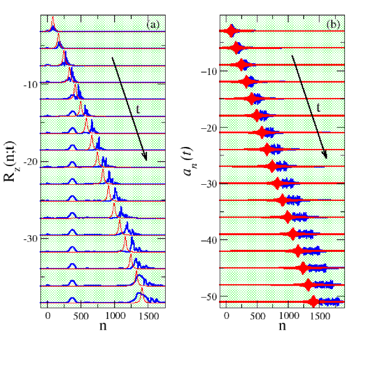
Figure 34: (a) Snapshots of the induced population inversion pulse $R_{z}(n;t)$, excited by the electromagnetic vector potential pulse $a_{n}(t)$, whose corresponding snapshots are shown in (b), for two-photon self-induced transparent (TPSIT, absorbing) superconducting quantum metamaterials. (b) Snapshots of the corresponding electromagnetic vector potential pulse $a_{n}(t)$. In both (a) and (b), the numerically obtained pulses are shown in blue color, while the analytical solutions are shown in red color. Parameters: $\chi=1/5$, $\beta=6$, $V_{00}=V_{11}=1$, $V_{01}=V_{10}=0.8$, $E_{1}-E_{0}=3$, and $v/c=0.7$. Only a small part of the simulated array of SCQs is shown for clarity.

The situation seems to be different, however, in the case of two-photon superradiant (SRD) pulses, as can be observed in the snapshots shown in Figs. 35a and b, for $R_{z}(n;t)$ and $a_{n}(t)$, respectively. Here, the lack of the direct interaction between SCQs is crucial, since the SCQs that make a transition from the excited to their ground state as the peak of the $a_{n}(t)$ pulse passes by their location, cannot return to their excited states after the $a_{n}(t)$ pulse has gone away. It seems, thus, that the $a_{n}(t)$ pulse excites a kink-like $R_{z}(n;t)$ front that propagates along with it at the same velocity. It should be noted that the common velocity of the $R_{z}(n;t)$ kink and the $a_{n}(t)$ pulse is considerably lower than the analytically predicted one, as it can be observed in Figs. 35a and b. Even more complicated behavioral patterns of two-photon SRD propagating pulses have been also obtained ¹⁵¹. The effect of non-zero $\gamma$ factor on the $R_{z}(n;t)$ and $a_{n}(t)$ pulses is clearly revealed in Fig. 36. These snapshots are taken at instants eparated by $14$ time-units, from $t=0$ to $t=168$. They are shifted downwards to avoid overlapping, and only part of the array is shown for clarity. A small value of the factor $\gamma$ ($\gamma=0.01$) has practically negligible effect on the $R_{z}(n;t)$ and $a_{n}(t)$ pulses (Figs. 36a and b). However, when $\gamma$ increases (e.g., to $\gamma=0.1$, as in Figs. 36c and d), the amplitude of the envelop of the $R_{z}(n;t)$ pulse decreases significantly. For even higher values of $\gamma$, the excitation of $R_{z}(n;t)$ pulses becomes impossible.

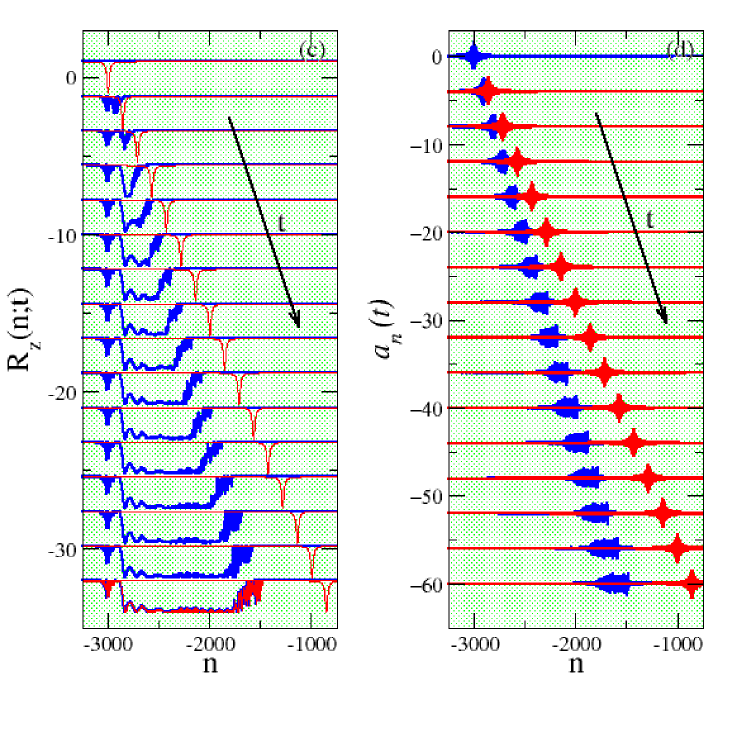
Figure 35: (a) Snapshots of the induced population inversion pulse $R_{z}(n;t)$, excited by the electromagnetic vector potential pulse $a_{n}(t)$, whose corresponding snapshots are shown in (b), for two-photon superradiant (TPSRD, amplifying) superconducting quantum metamaterials. (b) Snapshots of the electromagnetic vector potential pulse $a_{n}(t)$. In both (a) and (b), the numerically obtained pulses are shown in blue color, while the analytical solutions are shown in red color. Parameters: $\chi=1/5$, $\beta=6$, $V_{00}=V_{11}=1$, $V_{01}=V_{10}=0.8$, $E_{1}-E_{0}=3$, and $v/c=0.7$. Only a small part of the simulated array of SCQs is shown for clarity.

Thus, even for non-zero $\gamma$, an $a_{n}(t)$ pulse is able to excite or induce $R_{z}(n;t)$ pulse whose amplitude gradually increases until it attains its maximum value; that value is close to but less than unity for a small but non-zero $\gamma$ (e.g., for $\gamma=0.01$ as in Fig. 36a and b). The induced $R_{z}(n;t)$ pulse propagates along with the $a_{n}(t)$ pulse with velocity $v^{\prime}$. In Fig. 36a, the amplitude of the $R_{z}(n;t)$ pulse reaches its maximum at $t\simeq 70$ time units; subsequently it evolves in time while it keeps its amplitude almost constant for at least the next $56$ time-units. After that, its amplitude starts decreasing until it is completely smeared (not shown). During the time interval in which the amplitude of the $R_{z}(n;t)$ pulse is close to (but less than) unity, the SCQMM is considered to be in an almost coherent regime. Note that at about $t=84$ a little bump starts to appear which grows to a little larger one as time advances (”probability bump”). This probability bump, as well as that observed also in Fig. 34a for a different parameter set which gives $\gamma=0$, is immobile and its peak is located on a site around $n\sim 300$. A second such bump appears at $n=0$ due to the initial ”shock” of the qubit subsystem because of the sudden onset of the $a_{n}(t)$ pulse. A comparison of the numerical $R_{z}(n;t)$ profiles with the analytical ones reveals that the velocity of propagation $v^{\prime}$, the same for the numerically onbtained $R_{z}(n;t)$ and $a_{n}(t)$ pulses, (Figs. 36a and b), is slightly larger than the analytically obtained one $v$ ($v^{\prime}>v$). In Figs. 36c and d, the diagonal effective matrix interaction elements $V_{ij}$ ($i,j=0,1$) have been chosen so that the factor $\gamma$ has the value of $0.1$. That value is obtained by choosing, specifically, $V_{00}=0.98$, $V_{11}=1.02$, and $V_{01}=V_{10}=0.7$, and it is already high enough to Stark-shift considerably the energy levels of the SCQs. The effect of $\gamma=0.1$ becomes apparent by comparing Figs. 36a and b, with Figs. 36c and d, respectively. Remarkably, the EM vector potential pulse $a_{n}(t)$ does not seem to be affected significantly. However, the numerically obtained, induced population inversion pulse $R_{z}(n;t)$ has much lower amplitude compared with that of the analytically predicted form which is only slightly affected by the high value of $\gamma$. Note that the speed of the $R_{z}(n;t)$ pulse is the same as that in the case of lower value of $\gamma$ ($\gamma=0.01$). Even the unwanted ”probability bumps” in Figs. 36a and c, for $\gamma=0.01$ and $0.1$, respectively, appear at about the same locations with almost the same amplitude and shape.

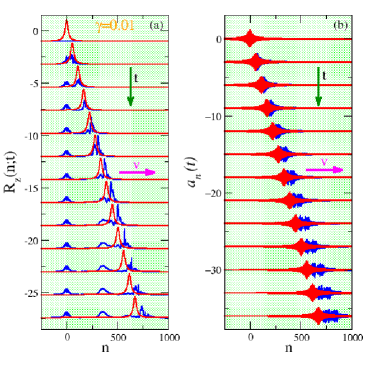
Figure 36: Snapshots of the induced population inversion pulse $R_{z}(n;t)$ and the electromagnetic vector potential pulse $a_{n}(t)$ in two-photon self-induced transparent (TPSIT, absorbing) superconducting quantum metamaterials for a non-zero $\gamma$ factor. (a) Snapshots of $R_{z}(n;t)$ for $\gamma=0.01$ ($V_{00}=0.998$, $V_{11}=1.002$). (b) Snapshots of $a_{n}(t)$ which excite the corresponding $R_{z}(n;t)$ pulses in (a). (c) Snapshots of $R_{z}(n;t)$ for $\gamma=0.1$ ($V_{00}=0.98$, $V_{11}=1.02$). (d) Snapshots of $a_{n}(t)$ which excite the corresponding $R_{z}(n;t)$ pulses in (c). The other parameters are: $\chi=1/4.9$, $\beta=6$, $V_{01}=V_{10}=0.7$, $E_{1}-E_{0}=3$, and $v/c=0.7$. In (a)-(d), the numerically obtained pulses are shown in blue color, while the analytical solutions are shown in red color. Only a small part of the simulated array of SCQs is shown for clarity.

6 Summary

SQUIDs metamaterials exploit geometry, superconductivity, and the Josephson effect, to exhibit extraordinary metamaterial properties and very rich dynamic behavior. Many aspects of their behavior have been investigated both theoretically and experimentally; properties such as negative diamagnetic permeability, wide-band tunability of the resonance either by a magnetic field or the temperature, fast switching between multistable states, broad-band self-induced transparency, and coherent oscillations, have been experimentally observed. Moreover, some of these properties have been numerically confirmed. Further theoretical results, which relay primarily on numerical simulations, have predicted the existence of nonlinearly localized states in the form of discrete breathers, the existence the counter-intuitive chimera states, the nonlinear band opening, and the existence of flat-band localized modes, the latter in SQUID metamaterials on Lieb lattices. All the above results presented in this review have been obtained in the classical regime, although even those phenomenological, equivalent circuit models used to simulate SQUID metamaterials, encompass macroscopic quantum effects. In the quantum regime, a particular paradigmatic model describing an array of superconducting charge qubits periodically loaded in a superconducting transmission line, has been reviewed. That system could be also regarded as an array of SQUIDs, which SQUIDs however are strongly coupled to each other through direct conducting paths. For that superconducting quantum metamaterial, the possibility for the opening of an oscillating photonic band gap, the propagation of self-induced transparent and superradiant pulses, and the induction of quantum coherence in the qubit chain by the propagating pulses, has been theoretically demonstrated.

The presented review cannot be exhaustive on SQUID metamaterials and quantum superconducting metamaterials, since that area of the field of metamaterial research evolves very fast; experiments on both classes of systems are going on that will perhaps reveal further surprising results. There was an attempt to guide the reader through the main results in this area, and to stress that the presented properties of the SQUID metamaterials are to a large extent a result of nonlinearity of their elementary units, i.e., the individual SQUIDs. Indeed, substantial nonlinearity leads to multistability in a single SQUID for driving frequencies close to its resonance. That resonance can be tuned by a dc and/or a harmonic field; moreover, the amplitude of the latter also determines the strength of the nonlinearity. The SQUID metamaterials, inherit to a large degree the properties of their elements; moreover, the complexity of their dynamics increases immensely in the multistability region with increasing the number of SQUIDs. That makes possible the appearance of collective states such as the chimera states. The nonlinearity of individual SQUIDs is also responsible for the localization of energy leading to the generation of discrete breathers which exist due to a delicate balance between intrinsic dissipation and incoming power from the external field (dissipative breathers). The flat-band localized modes, on the other hand, may exist due to the particular lattice geometry (Lieb lattice), in the linear regime (very low field intensities).

For the superconducting quantum metamaterials, the Josephson nonlinearity is again crucial in order to form a particular type of a superconducting qubit, i.e., an effectively two-level system (by neglecting all the other, higher energy states). Those qubits, couple through their Josephson junction(s) to the magnetic component of the electromagnetic field of a pulse launched form one end; that interaction allows for the generation of important quantum optical effects, such as self-induced transparency and superradiance. Moreover, the propagating pulses, which are shaped to acquire Lorentzian profiles, are able to induce quantum coherence in the form of population inversion pulses of the same shape in the qubit chain. Also, proper design of the qubit parameters allows for controlling the (common) speed of the propagating pulses in the superconducting quantum metamaterial, which is not possible in a natural material.

Appendix A Derivation of the Maxwell-Bloch-sine-Gordon equations

A.1 Quantization of the Qubit Subsystem

Consider an infinite number of superconducting charge qubits (SCQs) of the form of mesoscopic superconducting islands, periodically loaded in a transmission line (TL) that consists of two superconducting plates separated by distance $d$. The center-to-center distance between the qubits, $\ell$, is of the same order of magnitude as $d$. The SCQs are connected to each electrode of the TL with a Josephson junction (JJ). Assume that an electromagnetic (EM) wave corresponding to a vector potential $\vec{A}=A_{z}(x,t)\hat{z}$ which propagates along that superconducting TL, in a direction parallel to the electrodes and perpendicular to the direction of propagation of the EM wave. In the following it is assumed that the wavelength $\lambda$ of the EM field is much larger than the other length scales such as the separation of the electrodes $d$ and the distance between SCQs $\ell$, i.e., $\lambda>>\ell,d$. Then, the magnitude of the EM vector potential component $A_{z}(x,t)$ is approximatelly constant within a unit cell, so that $A_{z}(x,t)\simeq A_{z,n}(t)$. The Hamiltonian of the compound qubit array - EM field system shown in Fig. 32 of the paper is then

$$H=\sum_{n}\left\{\dot{\varphi}^{2}_{n}-2\cos\alpha_{n}\cos\varphi_{n}+\dot{\alpha}^{2}_{n}+\beta^{2}(\alpha_{n+1}-\alpha_{n})^{2}\right\},$$ (130)

where $\varphi_{n}$ is the superconducting phase on $n-$th island, $\beta^{2}=(8\pi dE_{J})^{-1}\left(\Phi_{0}/(2\pi)\right)^{2}$, $a_{n}(t)=(2\pi d/\Phi_{0})A_{n}(t)$ is the normalized and discretized EM vector potential at the $n-$th unit cell, and the overdots denote derivation with respect to time $t$. The Hamiltonian Eq. (130) is given in units of the Josephson energy $E_{J}=(\Phi_{0}I_{c})/(2\pi C)$, where $I_{c}$ and $C$ is the critical current and capacitance, respectively, of the JJs, and $\Phi_{0}=h/(2e)$ is the flux quantum, with $h$ and $e$ being the Planck’s constant and the electron charge, respectively. By adding and subtracting $2\cos\phi_{n}$ to the Hamiltonian $H$ and subsequently rearranging, we get the more transparent form

$$H=H_{qub}+H_{emf}+H_{int},$$ (131)

where the qubit subsystem energy $H_{qub}$, the EM field energy $H_{emf}$, and their interaction energy $H_{int}$, take respectively the form

$$H_{qub}=\sum_{n}\{\dot{\varphi}^{2}_{n}-2\cos\varphi_{n}\},\qquad H_{emf}=\sum_{n}\{\dot{\alpha}^{2}_{n}+\beta^{2}(\alpha_{n+1}-\alpha_{n})^{2}\},\qquad H_{int}=\sum_{n}\{2\cos\varphi_{n}(1-\cos\alpha_{n})\}.$$ (132)

In order to quantize the qubit subsystem, the classical variables $\varphi_{n}$ and $\dot{\varphi}_{n}$ are replaced by the quantum operators $\hat{\varphi_{n}}$ and $\dot{\varphi}_{n}\rightarrow-i\frac{\partial}{\partial\varphi_{n}}$, respectively, in $H_{qub}$ and $H_{int}$. The exact energy spectrum $E_{p}(n)$ and the corresponding wavefunctions $\Xi_{p}(n)$ of the $n$th qubit may then be obtained by mapping the Schrödinger equation with its Hamiltonian $H_{qub,n}=\dot{\varphi}_{n}^{2}-2\cos\varphi_{n}$, onto the Mathieu equation

$$\bigg{(}\frac{\partial^{2}}{\partial\varphi^{2}_{n}}+E_{p,n}-2\cos\varphi_{n}\bigg{)}\Xi_{p,n}=0.$$ (133)

Since the qubits are identical and non-interacting directly, the second quantization of the qubit subsystem proceeds as follows (the subscript $n$ is dropped): First $H_{qub}$ is written as

$$H_{qub}=-\int d\varphi_{n}\hat{\Psi}^{\dagger}(\varphi)\bigg{(}\frac{\partial^{2}}{\partial\varphi^{2}}+2\cos\varphi\bigg{)}\hat{\Psi}(\varphi),$$ (134)

where $\hat{\Psi}^{\dagger}$ and $\hat{\Psi}$ are field operators. Then, using the expansion $\hat{\Psi}(\varphi)=\sum_{p}a_{p}\Xi_{p}(\varphi)$, where the operators $a^{\dagger}_{p}$ ($a_{p}$) create (annihilate) qubit excitations of energy $E_{p}$, the Hamiltonian Eq. (134) is transformed into

$$H_{qub}=\sum_{p=0,1,...}E_{p}a^{\dagger}_{p}a_{p}.$$ (135)

We hereafter restrict $H_{qub}$ to the Hilbert subspace of its two lowest levels, i.e., those with $p=0,1$, so that in second quantized form the Hamiltonian Eqs. (131) and (132) read

$$H=\sum_{n}\sum_{p}E_{p}(n)a^{\dagger}_{n,p}a_{n,p}+\sum_{p,p^{\prime}}V_{p,p^{\prime}}(n)a^{\dagger}_{n,p}a_{n,p^{\prime}}\sin^{2}\frac{\alpha_{n}}{2}+\sum_{n}\{\dot{\alpha}^{2}_{n}+\beta^{2}(\alpha_{n+1}-\alpha_{n})^{2}\},$$ (136)

where $p,p^{\prime}=0,1$ and

$$V_{p,p^{\prime}}(n)\equiv V_{p^{\prime},p}(n)=\int d\varphi_{n}\Xi^{*}_{p}(\varphi_{n})\cos\varphi_{n}\Xi_{p,n}(\varphi_{n}),$$ (137)

are the matrix elements of the $n$th qubit - EM field interaction. In the reduced state space, in which a single qubit can be either in the ground ($p=0$) or in the excited ($p=1$) state, the normalization condition $\sum_{p}a^{\dagger}_{n,p}a_{n,p}=1$ holds for any $n$.

A.2 Maxwell-Bloch Formulation of the Dynamic Equations

In accordance with the semiclassical approach adopted here, the time-dependent Schrödinger equation

$$i\hbar\frac{\partial}{\partial t}|\Psi\rangle=\bar{H}|\Psi\rangle,$$ (138)

in which $\bar{H}$ is the Hamiltonian from Eq. (136) in physical units, i.e., $\bar{H}=HE_{J}$, is employed for the description of the qubit subsystem. The state of each qubit is a superposition of the form

$$|\Psi_{n}\rangle=\sum_{p}\Psi_{n,p}(t)a^{\dagger}_{n,p}|0\rangle,$$ (139)

whose coefficients $\Psi_{n,p}$ satisfy the normalization conditions

$$\sum_{p}|\Psi_{n,p}(t)|^{2}=1,\qquad\sum_{n,p}|\Psi_{n,p}(t)|^{2}=N,$$ (140)

in which a finite $N-$qubit subsystem is implied. Assuming that the pulse power is not very strong, the approximation $[1-\cos(\alpha_{n})]\simeq(1/2)\alpha^{2}_{n}$ can be safely applied in the interaction part of the Hamiltonian $H_{int}$. Then, the substitution of $|\Psi\rangle=|\Psi_{n}\rangle$ from Eq. (139) into the Schrödinger equation (138), and the derivation of the classical Hamilton’s equation for the normalized EM vector potential $\alpha_{n}$, yields

$$i\dot{\Psi}_{n,p}=\epsilon_{p}\Psi_{n,p}+\frac{1}{\chi}\sum_{p^{\prime}}V_{p,p^{\prime}}(n){\Psi}_{n,p^{\prime}}\alpha^{2}_{n},$$ (141)

$$\ddot{\alpha}_{n}-\beta^{2}(\alpha_{n+1}+\alpha_{n-1}-2\alpha_{n})+\sum_{p,p^{\prime}}V_{p,p^{\prime}}\Psi^{*}_{n,p}\Psi_{n,p^{\prime}}\alpha_{n}=0,$$ (142)

where $\chi=\hbar\omega_{J}/E_{J}$. In Eqs. (141) and (142), the temporal variable is renormalized according to $t\rightarrow\omega_{J}t$ and thus the dimensionless energy of the qubit excitations is redefined according to $E_{P}\rightarrow\epsilon_{p}=E_{p}/\chi$.

The evolution Eqs. (141) and (142) can be rewritten in terms of the $n-$dependent Bloch vector components through the transformation

$$R_{z}(n)=|\Psi_{n,1}|^{2}-|\Psi_{n,0}|^{2},\qquad R_{y}(n)=i(\Psi^{*}_{n,0}\Psi_{n,1}-\Psi^{*}_{n,1}\Psi_{n,0}),\qquad R_{x}(n)=\Psi^{*}_{n,1}\Psi_{n,0}+\Psi^{*}_{n,0}\Psi_{n,1},$$ (143)

in which the variables $R_{i}$ ($i=x,y,z$) apply to each single qubit, as

$$\dot{R}_{x}(n)=-(\Delta+2D\alpha_{n}^{2})R_{y}(n),\qquad\dot{R}_{y}(n)=+(\Delta+2D\alpha_{n}^{2})R_{x}(n)-2\mu\alpha_{n}^{2}R_{z}(n),\qquad\dot{R}_{z}(n)=+2\mu\alpha_{n}^{2}R_{y}(n),$$ (144)

$$\ddot{\alpha}_{n}+\chi[\Omega^{2}+\mu R_{x}(n)+DR_{z}(n)]\alpha_{n}=\beta^{2}(\alpha_{n-1}-2\alpha_{n}+\alpha_{n+1}),$$ (145)

where $D=\frac{(V_{11}-V_{00})}{2\chi}$, $\Omega^{2}=\frac{(V_{11}+V_{00})}{2}$, $\mu=\frac{V_{10}}{\chi}$, and $\Delta=\epsilon_{1}-\epsilon_{0}\equiv\frac{(E_{1}-E_{0})}{\chi}$. By taking the continuous limit of Eqs. (144) and (145), we obtain

$$\dot{R}_{x}=-(\Delta+2D\alpha^{2})R_{y},\qquad\dot{R}_{y}=+(\Delta+2D\alpha^{2})R_{x}-2\mu\alpha^{2}R_{z},\qquad\dot{R}_{z}=+2\mu\alpha^{2}R_{y},$$ (146)

$$\ddot{\alpha}-\beta^{2}\alpha_{xx}+\Omega^{2}\alpha=-\chi(DR_{z}+\mu R_{x})\alpha,$$ (147)

where $R_{x}$, $R_{y}$, $R_{z}$, and $\alpha$ are functions of the spatial variable $x$ and the normalized temporal variable $t$, while the overdots denote partial derivation with respect to the latter. The Bloch equations (146) possess the dynamic invariant $\sum_{i}R^{2}_{i}=1$.

A.3 Slowly Varying Envelope Approximation and Reduced Dynamic Equations

The Slowly Varying Envelope Approximation (SVEA) relies on the assumption that the envelop of a travelling pulse in a nonlinear medium varies slowly in both time and space compared with the period of the carrier wave, which makes possible to introduce slow and fast variables. According to the SVEA, the EM vector potential can be approximated as

$$\alpha(x,t)=\varepsilon(x,t)\cos\psi(x,t),$$ (148)

where $\psi(x,t)=kx-\omega t+\phi(x,t)$, with $k$ and $\omega$ being the wavenumber and frequency of the carrier wave, respectively, which depend on each other through the dispersion relation, and $\varepsilon(x,t)$ and $\phi(x,t)$ are the slowly varying envelop and phase, respectively. Using fast and slow variables, the $x$ and $y$ Bloch vector components, $R_{x}(n)$ and $R_{y}(n)$, can be expressed as a function of new, in-phase and out-of-phase Bloch vector components $r_{x}$ and $r_{y}$ as

$$R_{x}=r_{x}\cos(2\psi)+r_{y}\sin(2\psi),\qquad R_{y}=r_{y}\cos(2\psi)-r_{x}\sin(2\psi),\qquad R_{z}=r_{z}.$$ (149)

From Eqs. (148) and (149), the second temporal and spatial derivative of $\alpha(x,t)$ can be approximated by

$$\ddot{\alpha}\approx 2\omega\dot{\varepsilon}\sin\psi+(2\omega\dot{\phi}-\omega^{2})\varepsilon\cos\psi,\qquad\alpha_{xx}\approx-2k\varepsilon_{x}\sin\psi-(2k\phi_{x}-k^{2})\varepsilon\cos\psi,$$ (150)

in which the rapidly varying terms of the form $\ddot{\varepsilon}$, $\varepsilon_{xx}$, $\phi^{2}$, $\phi_{xx}$, $\ddot{\phi}$, $\phi_{x}\varepsilon_{x}$, etc., have been neglected. Substitution of Eqs. (150) and (149), into Eq. (147) gives

$$2(\omega\dot{\varepsilon}+k\beta^{2}\varepsilon_{x})\sin\psi+[2(\dot{\phi}\omega+k\phi_{x})-\omega^{2}+\Omega^{2}+\beta^{2}k^{2}]\varepsilon\cos\psi=-\chi\{Dr_{z}+\mu[r_{x}\cos(2\psi)+r_{y}\sin(2\psi)]\}\varepsilon\cos\psi.$$ (151)

Equating the coefficients of $\sin\psi$ and $\cos\psi$ in the earlier equation yields

$$\omega\dot{\varepsilon}+k\beta^{2}\varepsilon_{x}=-\chi\mu r_{y}\varepsilon\cos^{2}\psi,$$ (152)

and

$$2(\dot{\phi}\omega+k\phi_{x})-\{\omega^{2}-\Omega^{2}-\beta^{2}k^{2}\}=-\chi[Dr_{z}+\mu r_{x}\cos(2\psi)].$$ (153)

The dispersion relation $\omega=\omega(k)$ is obtained from Eq. (153) by zeroing the expression in the curly brackets as

$$k=\pm\frac{\sqrt{\omega^{2}-\Omega^{2}}}{\beta}.$$ (154)

Thus, EM waves propagate through the superconducting quantum metamaterial (SCQMM) only when their frequency exceeds a critical one, $\omega_{c}=\Omega=\sqrt{(V_{00}+V_{11})/2}$. Finally, Eqs. (152) and (153) are averaged in time over the period of the fast time-scale $T=2\pi/\omega$ of the phase $\psi(x,t)$. Due to the assumed time-dependence of $\psi(x,t)$ within the SVEA framework, that averaging requires the calculation of integrals of the form

$$\langle{\cal F}(\sin f(\psi),\cos g(\psi))\rangle=\frac{1}{2\pi}\int^{2\pi}_{0}{\cal F}(\sin f(\psi),\cos g(\psi))d\psi.$$

This procedure, when it is applied to the two evolution Eqs. (152) and (153) provides the truncated equations for slow amplitude and phase

$$\dot{\varepsilon}+c\varepsilon_{x}=-\chi\frac{\mu}{2\omega}\varepsilon r_{y},\qquad\dot{\phi}+c\phi_{x}=-\chi\frac{D}{\omega}R_{z},$$ (155)

where $c=\beta^{2}k/\omega$ is a critical velocity.

Substituting Eq. (148) and (149) into Eqs. (146) for the original Bloch vector components, we get

$$(\dot{r}_{x}+2\dot{\psi}r_{y})\cos(2\psi)+(\dot{r}_{y}-2\dot{\psi}r_{x})\sin(2\psi)=-(\Delta+2D\varepsilon^{2}\cos^{2}\psi)[r_{y}\cos(2\psi)-r_{x}\sin(2\psi)]i$$ (156)

$$(\dot{r}_{y}-2\dot{\psi}r_{x})\cos(2\psi)-(\dot{r}_{x}+2\dot{\psi}r_{y})\sin(2\psi)=(\Delta+2D\varepsilon^{2}\cos^{2}\psi)[r_{x}\cos(2\psi)+r_{y}\sin(2\psi)]-2\mu\varepsilon^{2}\cos^{2}\psi r_{z}$$ (157)

$$\dot{r}_{z}=2\mu\varepsilon^{2}\cos^{2}\psi[r_{y}\cos(2\psi)-r_{x}\sin(2\psi)].$$ (158)

By multiplication of Eqs. (156) and (157) by $\cos(2\psi)$ and $\sin(2\psi)$, respectively, and subsequent subtraction of the one equation from the other, we get

$$\dot{r}_{x}+2\dot{\psi}r_{y}=-(\Delta+2D\varepsilon^{2}\cos^{2}\psi)r_{y}+2\mu\varepsilon^{2}\cos^{2}\psi\cos(2\psi)r_{z}.$$ (159)

Similarly, by multiplication of Eqs. (156) and (157) by $\sin(2\psi)$ and $\cos(2\psi)$, respectively, and subsequent addition of the resulting equations, we get

$$\dot{r}_{y}-2\dot{\psi}r_{x}=(\Delta+2D\varepsilon^{2}\cos^{2}\psi)r_{x}-2\mu\varepsilon^{2}\cos^{2}\psi\sin(2\psi)r_{z}.$$ (160)

The, performing an averaging of Eqs. (158)-(160) over the phase $\psi$ using the relations $\langle\cos^{2}\psi\cos(2\psi)\rangle=1/4$ and $\langle\cos^{2}\psi\sin(2\psi)\rangle=0$ yields the truncated Bloch equations

$$\dot{r}_{x}=-(\delta+2\dot{\phi}+D\varepsilon^{2})r_{y}-\frac{\mu}{2}\varepsilon^{2}r_{z},\qquad\dot{r}_{y}=+(\delta+2\dot{\phi}+D\varepsilon^{2})r_{x},\qquad\dot{r}_{z}=\frac{\mu}{2}\varepsilon^{2}r_{y},$$ (161)

where $\delta=\Delta-2\omega$. Eqs. (161) possess a dynamic invariant that has a form similar to that of the original Bloch equations (146), i.e., $r^{2}_{x}+r^{2}_{y}+r^{2}_{z}=1$. The truncated Bloch equations (161), along with Eqs. (155) for $\varepsilon(x,t)$ and $\phi(x,t)$ of the EM vector potential pulse, constitute a closed system of equations describing the approximate dynamics of the SCQMM. Its solutions are obtained in the next Section.

A.4 Exact Integration of the Truncated Equations

The combination of Eq. (155) and the third of Eqs. (161) provides a relation between the slow amplitude and the phase of the EM vector potential pulse. Multiplication of the first of Eqs. (155) by $\varepsilon$ gives

$${\left[\frac{\partial}{\partial t}+c\frac{\partial}{\partial x}\right]\varepsilon^{2}(x,t)}=-\chi\frac{\mu}{\omega}\varepsilon^{2}(x,t)r_{y}.$$ (162)

Subsequently, the time-derivative of the second of Eqs. (155), in which $\dot{R}_{z}=\dot{r}_{z}$ is replaced from the third of Eqs. (161), gives

$${\left[\frac{\partial}{\partial t}+c\frac{\partial}{\partial x}\right]\dot{\phi}(x,t)}=-\chi\frac{\mu D}{2\omega}\varepsilon^{2}(x,t)r_{y}.$$ (163)

From Eqs. (162) and (163), and by taking into account the independence of the slow temporal and spatial variables, we get

$$2\dot{\phi}(x,t)=D\varepsilon^{2}(x,t)+const.,$$ (164)

where the constant of integration can be set equal to zero. Using Eq. (164), the truncated Bloch equations (161) can be written as

$$\dot{r}_{x}=-(\delta+2D\varepsilon^{2})r_{y},\qquad\dot{r}_{y}=+(\delta+2D\varepsilon^{2})r_{x}-\frac{\mu}{2}\varepsilon^{2}r_{z},\qquad\dot{r}_{z}=\frac{\mu}{2}\varepsilon^{2}r_{y}.$$ (165)

The latter can be written in a simpler form using the unitary transformation

$$r_{x}=S_{x}\cos\Phi-S_{z}\sin\Phi,\qquad r_{y}=S_{y},\qquad r_{z}=S_{z}\cos\Phi+S_{x}\sin\Phi,$$ (166)

where $\Phi$ is a constant transformation angle (to be determined). The truncated Bloch equations for the $r_{i}$, $i=x,y,z$, can be written in terms of the new Bloch vector components $S_{i}$, using a procedure similar to that used in the previous Section to obtain Eqs. (161). Sustituting Eqs. (166) into Eqs. (165), we get

$$\dot{S}_{x}\cos\Phi-\dot{S}_{z}\sin\phi=-(\delta+2D\varepsilon^{2})S_{y},$$ (167)

$$\dot{S}_{y}=\left[(\delta+2D\varepsilon^{2})\cos\Phi-\frac{\mu}{2}\varepsilon^{2}\sin\Phi\right]S_{x}-\left[(\delta+2D\varepsilon^{2})\sin\Phi+\frac{\mu}{2}\varepsilon^{2}\cos\Phi\right]S_{z},$$ (168)

$$\dot{S}_{x}\sin\Phi+\dot{S}_{z}\cos\Phi=-\frac{\mu}{2}\varepsilon^{2}S_{y}.$$ (169)

Multiplying Eqs. (167) and (169) by $\cos\Phi$ and $\sin\Phi$, respectively, and then adding them together, we get

$$\dot{S}_{x}=\left\{\varepsilon^{2}\left[\frac{1}{2}\mu\sin\Phi-2D\cos\Phi\right]-\delta\cos\Phi\right\}S_{y}.$$ (170)

Similarly, multiplying Eqs. (167) and (169) by $\sin\Phi$ and $\cos\Phi$, respectively, and then subtracting the one equation from the other, we get

$$\dot{S}_{z}=\left\{\varepsilon^{2}\left[\frac{1}{2}\mu\cos\Phi+2D\sin\Phi\right]-\delta\sin\Phi\right\}S_{y}.$$ (171)

Let us define the transformation angle through the relation $\tan\Phi\equiv\gamma=\frac{4D}{\mu}$, so that $\cos\Phi=\pm\sigma$ and $\sin\Phi=\pm\sigma\gamma$ where $\sigma=1/\sqrt{1+\gamma^{2}}$. The choice of the sign is irrelevant and here we pick positive sign for both functions. Using that $\Phi$ and the definitions $W=\sqrt{(4D)^{2}+\mu^{2}}$ and $\eta=-\delta\mu/W$, Eqs. (170), (168), and (171) obtain their final form

$$\dot{S}_{x}=+\eta S_{y},\qquad\dot{S}_{y}=-\eta S_{x}+\left[\eta\gamma-\frac{1}{2}W\varepsilon^{2}\right]S_{z},\qquad\dot{S}_{z}=\left[-\eta\gamma+\frac{1}{2}W\varepsilon^{2}\right]S_{y}.$$ (172)

For the investigation of ”coherent propagation” of an EM potential pulse, the resonance condition is applied, i.e., $\eta=0$ or $\omega=\Delta/2$, and then Eqs. (172) become

$$\dot{S}_{x}=0,\qquad\dot{S}_{y}=-\frac{1}{2}W\varepsilon^{2}S_{z},\qquad\dot{S}_{z}=+\frac{1}{2}W\varepsilon^{2}S_{y}.$$ (173)

Combining the second and third of Eqs. (173) and integrating, we obtain the ”resonant” conservation law $S_{y}^{2}+S_{z}^{2}=const.$. Assuming that all the qubits are in the ground state at $t=-\infty$, we have the initial conditions $r_{x}(t=-\infty)=r_{y}(t=-\infty)=0$ and $r_{z}(t=-\infty)=-1$ which are transformed into $S_{x}(t=-\infty)=-\gamma\sigma$, $S_{y}(t=-\infty)=0$, and $S_{z}(t=-\infty)=-\sigma$ through Eq. (166). Applying the initial conditions to the resonant conservation law, we get

$$S_{y}^{2}+S_{z}^{2}=\sigma^{2}.$$ (174)

In the following, we seek solution of the form $\varepsilon=\varepsilon(\tau=t-x/v)$ and $S_{i}=S_{i}(\tau=t-x/v)$, with $i=x,y,z$. By changing the variables in the first of Eqs. (155), with $r_{y}$ being replaced by $S_{y}$, we get after rearramgement

$$\frac{\varepsilon_{\tau}}{\varepsilon}=\chi\frac{\mu}{2\omega}\frac{v}{c-v}S_{y}.$$ (175)

Then, combining Eq. (157) with the third of Eqs. (173) and integrating, we get

$$\varepsilon^{2}(\tau)=\chi\frac{2\mu}{\omega W}\frac{v}{c-v}[S_{z}(\tau)+\sigma],$$ (176)

where the conditions $\varepsilon(-\infty)$ and $S_{z}(-\infty)=-\sigma$ were used. The system of Eqs. (174)-(176) for $\varepsilon$, $S_{y}$, and $S_{z}$ can be integrated exactly; the variables $S_{y}$ and $S_{z}$ can be eliminated in favour of $\varepsilon$ to give $\varepsilon_{\tau}=\lambda\varepsilon^{2}\sqrt{a+b\varepsilon^{2}}$, in which the constants are defined as $a=2\sigma/\kappa$, $b=-1/\kappa^{2}$, $\lambda=\chi\frac{\mu}{2\omega}\frac{v}{c-v}$, $\kappa=\frac{2\mu}{\omega W}\frac{v}{c-v}$ to simplify the notation. The equation for $\varepsilon$ can be readily integrated

$$\int_{\varepsilon_{0}}^{\varepsilon}\frac{d\varepsilon}{\varepsilon^{2}\sqrt{a+b\varepsilon^{2}}}=\lambda\int_{\tau_{0}}^{\tau}d\tau\Rightarrow-\frac{\sqrt{a+b\varepsilon^{2}}}{a\varepsilon}=\lambda(\tau-\tau_{0}),$$ (177)

where we have set $\varepsilon_{0}\equiv\varepsilon(\tau=\tau_{0})=\sqrt{2\sigma\kappa}$ to eliminate the boundary term resulting from the integral over $\varepsilon$. Solving Eq. (177) for $\varepsilon$, we finally get a Lorentzian-like slowly varying amplitude

$$\varepsilon(\tau)=\frac{\varepsilon_{0}}{\sqrt{1+\tau_{p}^{-2}(\tau-\tau_{0})^{2}}},$$ (178)

where $\varepsilon_{0}=\sqrt{-{a}/{b}}=\sqrt{2\sigma\kappa}$ and

$$\tau_{p}^{-2}=-\frac{a^{2}\lambda^{2}}{b}=\left(\chi\frac{\sigma\mu}{\omega}\right)^{2}\left(\frac{v}{c-v}\right)^{2}.$$ (179)

References

- Schurig et al. [2006] Schurig D, Mock JJ, Justice BJ, Cummer SA, Pendry JB, Starr AF, Smith DR. Metamaterial electromagnetic cloak at microwave frequencies. Science 2006;314:977–980.
- Pendry [2000] Pendry JB. Negative refraction makes a perfect lens. Phys Rev Lett 2000;85:3966–3969.
- Linden et al. [2006] Linden S, Enkrich C, Dolling G, Klein MW, Zhou J, Koschny T, Soukoulis CM, Burger S, Schmidt F, Wegener M. Photonic metamaterials: magnetism at optical frequencies. IEEE J Selec Top Quant Electron 2006;12:1097–1105.
- Papasimakis et al. [2008] Papasimakis N, Fedotov VA, Zheludev NI, Prosvirnin SL. Metamaterial analog of electromagnetically induced transparency. Phys Rev Lett 2008;101:253903.
- Kurter et al. [2011a] Kurter C, Tassin P, Zhang L, Koschny T, Zhuravel AP, Ustinov AV, Anlage SM, Soukoulis CM. Classical analogue of electromagnetically induced transparency with a metal-superconductor hybrid metamaterial. Phys Rev Lett 2011a;107:043901.
- Jin et al. [2013] Jin BB, Wu JB, Zhang CH, Jia XQ, Jia T, Kang L, Chen J, Wu PH. Enhanced slow light in superconducting electromagnetically induced transparency metamaterials. Supercond Sci Technol 2013;26:074004 (5pp).
- Zhang et al. [2017a] Zhang C, Wu J, Jin B, Jia X, Kang L, Xu W, Wang H, Chen J, Tonouchi M, Wu P. Tunable electromagnetically induced transparency from a superconducting terahertz metamaterial. Appl Phys Lett 2017a;110:241105.
- Li et al. [2017] Li C, Wu J, Jiang S, Su R, Zhang C, Jiang C, Zhou G, Jin B, Kang L, Xu W, Chen J, Wu P. Electrical dynamic modulation of thz radiation based on superconducting metamaterials. Appl Phys Lett 2017;111:092601.
- Zheludev [2010] Zheludev NI. The road ahead for metamaterials. Science 2010;328:582–583.
- Zheludev [2011] Zheludev NI. A roadmap for metamaterials. Optics and Photonics News 2011;22:31–35.
- Tong [2018] Tong XC. Functional Metamaterials and Metadevices, Springer Series in Materials Science Vol.262. Springer International Publishing AG 2018; 2018.
- Smith et al. [2000] Smith DR, Padilla WJ, Vier DC, Nemat-Nasser SC, Schultz S. Composite medium with simultaneously negative permeability and permittivity. Phys Rev Lett 2000;84 (18):4184–4187.
- Shelby et al. [2001] Shelby RA, Smith DR, Schultz S. Experimental verification of a negative index of refraction. Science 2001;292:77–79.
- Wood and Pendry [2007] Wood B, Pendry JB. Metamaterials at zero frequency. J Phys: Condens Matter 2007;19:076208.
- Magnus et al. [2008] Magnus F, Wood B, Moore J, Morrison K, Perkins G, Fyson J, Wiltshire MCK, Caplini D, Cohen LF, Pendry JB. A d.c. magnetic metamaterial. Nature Mater 2008;7:295–297.
- Navau et al. [2009] Navau C, Chen DX, Sanchez A, Del-Valle N. Magnetic properties of a dc metamaterial consisting of parallel square superconducting thin plates. Appl Phys Lett 2009;94 (24):242501 (3 pages).
- Mawatari et al. [2012] Mawatari Y, Navau C, Sanchez A. Two-dimensional arrays of superconducting strips as dc magnetic metamaterials. Phys Rev B 2012;85:134524 [9 pages].
- Mach-Batlle et al. [2017] Mach-Batlle R, Parra A, Prat-Camps J, Laut S, Navau C, Sanchez A. Negative permeability in magnetostatics and its experimental demonstration. Phys Rev B 2017;96:094422.
- Yen et al. [2004] Yen TJ, Padilla WJ, Fang N, Vier DC, Smith DR, Pendry JB, Basov DN, Zhang X. Terahertz magnetic response from artificial materials. Science 2004;303:1494–1496.
- Linden et al. [2004] Linden S, Enkrich C, Dolling G, Klein MW, Zhou J, Koschny T, Soukoulis CM, Burger S, Schmidt F, Wegener M. Magnetic response of metamaterials at 100 terahertz. Science 2004;306:1351–1353.
- Withayachumnankul and Abbott [2009] Withayachumnankul W, Abbott D. Metamaterials in the terahertz regime. IEEE Photonics Journal 2009;1 (2):99–118.
- Gu et al. [2010] Gu J, Singh R, Tian Z, Cao W, Xing Q, He MX, Zhang JW, Han J, Chen H, Zhang W. Terahertz superconductor metamaterial. Appl Phys Lett 2010;97:071102 (3pp).
- Jin et al. [2010] Jin B, Zhang C, Engelbrecht S, Pimenov A, Wu J, Xu Q, Cao C, Chen J, Xu W. Low loss and magnetic field-tunable superconducting terahertz metamaterials. Opt Express 2010;18:17504–17509.
- Chen et al. [2010] Chen HT, Yang H, Singh R, O’Hara JF, Azad AK, Stuart A, Trugman SA, Jia QX, Taylor AJ. Tuning the resonance in high-temperature superconducting terahertz metamaterials. Phys Rev Lett 2010;105:247402–4.
- C. H. Zhang et al. [2013] C. H. Zhang BBJ, Han J, Kawayama I, Murakami H, Wu JB, Kang L, Chen J, Wu PH, Tonouchi M. Terahertz nonlinear superconducting metamaterials. Appl Phys Lett 2013;102:081121 (4 pages).
- Shalaev [2007] Shalaev VM. Optical negative-index metamaterials. Nature Photon 2007;1:41–48.
- Soukoulis et al. [2007] Soukoulis CM, Linden S, Wegener M. Negative refractive index at optical wavelengths. Science 2007;315:47–49.
- Litchinitser and Shalaev [2008] Litchinitser NM, Shalaev VM. Photonic metamaterials. Laser Phys Lett 2008;5:411–420.
- Veselago [1967] Veselago VG. The electrodynamics of substances with simultaneously negative values of epsilon and mu. Usp Fiz Nauk 1967;92:517–526.
- Pendry et al. [1999] Pendry JB, Holden AJ, Robbins DJ, Stewart WJ. Magnetism from conductors and enchanced nonlinear phenomena. IEEE Trans Microwave Theory Tech 1999;47:2075–2084.
- Pendry et al. [1996] Pendry JB, Holden AJ, Stewart WJ, Youngs I. Extremely low frequency plasmons in metallic mesostructures. Phys Rev Lett 1996;76:4773–4776.
- Caputo et al. [2012] Caputo JG, Gabitov I, Maimistov AI. Electrodynamics of a split-ring josephson resonator in a microwave line. Phys Rev B 2012;85:205446.
- Shamonina and Solymar [2004] Shamonina E, Solymar L. Magneto-inductive waves supported by metamaterials elements: components for a one-dimensinal waveguide. J Phys D: Appl Phys 2004;37:362–367.
- Butz et al. [2013a] Butz S, Jung P, Filippenko LV, Koshelets VP, Ustinov AV. A one-dimensional tunable magnetic metamaterial. Opt Express 2013a;21 (19):22540–22548.
- Zagoskin [2012] Zagoskin AM. Superconducting quantum metamaterials in 3d: possible realizations. J Opt 2012;14:114011 (4pp).
- Kafesaki et al. [2007] Kafesaki M, Tsiapa I, Katsarakis N, Koschny T, Soukoulis CM, Economou EN. Left-handed metamaterials: The fishnet structure and its variations. Phys Rev B 2007;75:235114.
- Wuestner et al. [2010] Wuestner S, Pusch A, Tsakmakidis KL, Hamm JM, Hess O. Overcoming losses with gain in a negative refractive index metamaterial. Phys Rev Lett 2010;105:127401 [4 pages].
- Liu et al. [2008] Liu N, Guo H, Fu L, Kaiser S, Schweizer H, Giessen H. Three-dimensional photonic metamaterials at optical frequencies. Nature Mater 2008;7:31–37.
- Valentine et al. [2008] Valentine J, Zhang S, Zentgraf T, Ulin-Avila E, Genov DA, Bartal G, Zhang X. Three-dimensional optical metamaterial with a negative refractive index. Nature 2008;455:376–379.
- Gay-Balmaz and Martin [2002] Gay-Balmaz P, Martin JFO. Electromagnetic resonances in individual and coupled split-ring resonators. J Appl Phys 2002;92:2929–2936.
- Hesmer et al. [2007] Hesmer F, Tatartschuk E, Zhuromskyy O, Radkovskaya AA, Shamonin M, Hao T, Stevens CJ, Faulkner G, Edwardds DJ, Shamonina E. Coupling mechanisms for split-ring resonators:theory and experiment. Phys Stat Sol (b) 2007;244:1170–1175.
- Penciu et al. [2008] Penciu RS, Aydin K, Kafesaki M, Koschny T, Ozbay E, Economou E, Soukoulis CM. Multi-gap individual and coupled split-ring resonator structures. Opt Express 2008;16:18131–18144.
- Liu et al. [2009] Liu N, Liu H, Zhu SN, Giessen H. Stereometamaterials. Nature Photon 2009;3:157–162.
- Sersić et al. [2009] Sersić I, Frimmer M, Verhagen E, Koenderink AF. Electric and magnetic dipole coupling in near-infrared split-ring metamaterial arrays. Phys Rev Lett 2009;103:213902.
- Liu and Giessen [2010] Liu N, Giessen H. Coupling effects in optical metamaterials. Angew Chem Int Ed 2010;49:9838–9852.
- Feth et al. [2010] Feth N, König M, Husnik M, Stannigel K, Niegemann J, Busch K, Wegener M, Linden S. Electromagnetic interaction of spit-ring resonators: The role of separation and relative orientation. Opt Express 2010;18:6545–6554.
- Syms et al. [2010] Syms RRA, Solymar L, Young IR, Floume T. Thin-film magneto-inductive cables. J Phys D: Appl Phys 2010;43:055102 (7pp).
- Wiltshire et al. [2003] Wiltshire MCK, Shamonina E, Young IR, Solymar L. Dispersion characteristics of magneto-inductive waves: comparison between theory and experiment. Electron Lett 2003;39:215–217.
- Dolling et al. [2006] Dolling G, Wegener M, Schädle A, Burger S, Linden S. Observation of magnetization waves in negative-index photonic metamaterials. Appl Phys Lett 2006;89:231118–3.
- Shadrivov et al. [2007] Shadrivov IV, Reznik AN, Kivshar YS. Magnetoinductive waves in arrays of split-ring resonators. Physica B 2007;394:180–184.
- Stevens et al. [2010] Stevens CJ, Chan CWT, Stamatis K, Edwards DJ. Magnetic metamaterials as 1-d data tranfer channels: An application for magneto-inductive waves. IEEE Trans Microw Theory Techniques 2010;58:1248–1256.
- Eleftheriades et al. [2002] Eleftheriades GV, Iyer AK, Kremer PC. Planar negative refractive index media using periodically lc loaded transmission lines. Microwave Theory and Techniques, IEEE Transactions on 2002;50 (12):2702–2712.
- Caloz and Itoh [2002] Caloz C, Itoh T. Application of the transmission line theory of left-handed (lh) materials to the realization of a microstrip. Antennas and Propagation Society International Symposium 2002;IEEE 2:412–415.
- Caloz [2009] Caloz C. Perspectives on em metamaterials. Materials Today 2009;2(3):12–20.
- Smith et al. [2004] Smith DR, Pendry JB, Wiltshire . Metamaterials and negative refractive index. Science 2004;Vol. 305 no. 5685:788–792.
- Caloz and Itoh [2005] Caloz C, Itoh T. Metamaterials for high-frequency electronics. Proceedings of the IEEE 2005;93 (10):1744–1752.
- Padilla et al. [2006] Padilla WJ, Basov DN, Smith DR. Negative refractive index metamaterials. Materials Today 2006;9 (7-8):28–35.
- Anlage [2011] Anlage SM. The physics and applications of superconducting metamaterials. J Opt 2011;13:024001–10.
- Soukoulis and Wegener [2011] Soukoulis CM, Wegener M. Past achievements and future challenges in the development of three-dimensional photonic metamaterials. Nature Photonics 2011;5:523–530.
- Liu and Zhang [2011] Liu Y, Zhang X. Metamaterials: a new frontier of science and technology. Chem Soc Rev 2011;40:2494–2507.
- Simovski et al. [2012] Simovski CR, Belov PA, Atrashchenko AV, Kivshar YS. Wire metamaterials: Physics and applications. Adv Mater 2012;24:4229–4248.
- Eleftheriades and Balmain [2005] Eleftheriades GV, Balmain KG. Negative-refraction metamaterials: Fundamental principles and applications. Wiley-IEEE Press; 2005.
- Caloz and Itoh [2006] Caloz C, Itoh T. Electromagnetic metamatrials: Transmission line theory and microwave applications. John Wiley Sons; 2006.
- Engheta and Ziokowski [2006] Engheta N, Ziokowski RW. Metamaterials: Physics and engineering explorations. Wiley-IEEE Press; 2006.
- Pendry [2007] Pendry JB. Fundamentals and applications of negative refraction in metamaterials. Princeton University Press; 2007.
- Marques et al. [2007] Marques R, Martin F, Sorolla M. Metamaterials with negative parameters. Hoboken, New Jersey: J. Wiley Sons; 2007.
- Krowne and Zhang [2007] Krowne CM, Zhang Y. Physics of negative refraction and negative index materials, optical and electronic aspects and diversified approaches. Springer; 2007.
- Ramakrishna and Grzegorczyk [2009] Ramakrishna SA, Grzegorczyk T. Physics and applications of negative refractive index materials. SPIE and CRC Press; 2009.
- Cui et al. [2010] Cui TJ, Smith DR, Liu R. Metamaterials theory, design and applications. Springer: Springer; 2010.
- Cai and Shalaev [2010] Cai W, Shalaev V. Optical metamaterials, fundamentals and applications. Heidelberg: Springer; 2010.
- Solymar and Shamonina [2009] Solymar L, Shamonina E. Waves in metamaterials. New York: Oxford University Press; 2009.
- Noginov and Podolskiy [2012] Noginov MA, Podolskiy VA. Tutorials in metamaterials. Taylor Francis; 2012.
- Fan and Padilla [2015] Fan K, Padilla WJ. Dynamic electromagnetic metamaterials. Materials Today 2015;18 (1):39–50.
- Lapine [2017] Lapine M. New degrees of freedom in nonlinear metamaterials. Phys Stat Sol (b) 2017;254 (4):1600462.
- Lapine et al. [2012] Lapine M, Shadrivov IV, Kivshar YS. Wide-band negative permeability of nonlinear metamaterials. Sci Rep 2012;2:412 (4pp).
- O’Brien et al. [2004] O’Brien S, McPeake D, Ramakrishna SA, Pendry JB. Near-infrared photonic band gaps and nonlinear effects in negative magnetic metamaterials. Phys Rev B 2004;69:241101(R).
- Hand and Cummer [2008] Hand TH, Cummer SA. Frequency tunable electromagnetic metamaterial using ferroelectric loaded split rings. J Appl Phys 2008;103:066105–3.
- Chen et al. [2006] Chen HT, Padilla WJ, Zide JMO, Gossard AC, Taylor AJ. Active terahertz metamaterial devices. Nature 2006;444:597–600.
- Powell et al. [2007] Powell DA, Shadrivov IV, Kivshar YS, Gorkunov MV. Self-tuning mechanisms of nonlinear split-ring resonators. Appl Phys Lett 2007;91:144107.
- Wang et al. [2008] Wang B, Zhou J, Koschny T, Soukoulis CM. Nonlinear properties of split-ring resonators. Opt Express 2008;16:16058.
- Shadrivov et al. [2008] Shadrivov IV, Kozyrev AB, van der Weide DW, Kivshar YS. Tunable transmission and harmonic generation in nonlinear metamaterials. Appl Phys Lett 2008;93:161903–3.
- Kozyrev and van der Weide [2008] Kozyrev AB, van der Weide DW. Nonlinear left-handed transmission line metamaterials. J Phys D: Appl Phys 2008;41:173001 (10pp).
- Jung et al. [2014a] Jung P, Ustinov AV, Anlage SM. Progress in superconducting metamaterials. Supercond Sci Technol 2014a;27:073001 (13pp).
- Esaki [1958] Esaki L. New phenomenon in narrow germanium junctions. Phys Rep 1958;109:603–605.
- Lazarides and Tsironis [2013a] Lazarides N, Tsironis GP. Gain-driven discrete breathers in symmetric nonlinear metamaterials. Phys Rev Lett 2013a;110:053901 (5pp).
- Rüter et al. [2010] Rüter CE, Makris KG, El-Ganainy R, Christodoulides DN, Segev M, Kip D. Observation of parity–time symmetry in optics. Nature Phys 2010;6:192–.
- Regensburger et al. [2012] Regensburger A, Bersch C, Miri MA, Onishchukov G, Christodoulides DN. Parity-time synthetic photonic lattices. Nature 2012;488:167–171.
- Bender and Boettcher [1998] Bender CM, Boettcher S. Real spectra in non-hermitian hamiltonians having symmetry. Phys Rev Lett 1998;80 (24):5243–5246.
- Bender et al. [2002] Bender CM, Brody DC, Jones HF. Complex extension of quantum mechanics. Phys Rev Lett 2002;89:270401.
- El-Ganainy et al. [2007] El-Ganainy R, Makris KG, Christodoulides DN, Musslimani ZH. Theory of coupled optical symmetric structures. Opt Lett 2007;32:2632–2634.
- Makris et al. [2008] Makris KG, El-Ganainy R, Christodoulides DN, Musslimani ZH. Beam dynamics in symmetric optical lattices. Phys Rev Lett 2008;100:103904.
- Boardman et al. [2007] Boardman AD, Rapoport YG, King N, Malnev VN. Creating stable gain in active metamaterials. J Opt Soc Am B 2007;24:A53–A61.
- Boardman et al. [2010] Boardman AD, Grimalsky VV, Kivshar YS, Koshevaya SV, Lapine M, Litchinitser NM, Malnev VN, Noginov M, Rapoport YG, Shalaev VM. Active and tunable metamaterials. Laser Photonics Rev 2010;5 (2):287–307.
- Xiao [2010] Xiao S. Loss-free and active optical negative-index metamaterials. Nature 2010;466:735.
- Jiang et al. [2011] Jiang T, Chang K, Si LM, Ran L, Xin H. Active microwave negative-index metamaterial transmission line with gain. Phys Rev Lett 2011;107:205503.
- Xu et al. [2012] Xu W, Padilla WJ, Sonkusale S. Loss compensation in metamaterials through embedding of active transistor based negative differential resistance circuits. Opt Express 2012;20:22406.
- Likharev. [1986] Likharev. KK. Dynamics of Josephson Junctions and Circuits. Philadelphia: Gordon and Breach; 1986.
- Narimanov [2008] Narimanov E. Photonics: Metamaterials to beat the static. Nature Mater 2008;7:273–274.
- Gömöry et al. [2012] Gömöry F, Solovyov M, Šouc J, Navau C, Prat-Camps J, Sanchez A. Experimental realization of a magnetic cloak. Science 2012;Vol. 335 no. 6075:1466–1468.
- Wu et al. [2011a] Wu JB, Jin BB, Wan J, Liang L, Zhang YG, Jia T, Cao CH, Kang L, Xu WW, Chen J, Wu PH. Superconducting terahertz metamaterials mimicking electromagnetically induced transparency. Appl Phys Lett 2011a;99:161113 (3 pages).
- Kurter et al. [2012] Kurter C, Tassin P, Zhuravel AP, Zhang L, Koschny T, Ustinov AV, Soukoulis CM, Anlage SM. Switching nonlinearity in a superconductor-enhanced metamaterial. Appl Phys Lett 2012;100:121906.
- Prat-Camps et al. [2013] Prat-Camps J, Sanchez A, Navau C. Superconductor–ferromagnetic metamaterials for magnetic cloaking and concentration. Supercond Sci Technol 2013;26:074001 (7pp).
- Wang et al. [2017] Wang D, Li C, Zhang C, Kang M, Zhang X, Jin B, Tian Z, Li Y, Zhang S, Han J, Zhang W. Superconductive symmetry phase transition in metasurfaces. Appl Phys Lett 2017;110:021104.
- Limberopoulos et al. [2009] Limberopoulos N, Akyurtlu A, Higginson K, Kussow AG, Merritt CD. Negative refractive index metamaterials in the visible spectrum based on mgb2/sic composites. Appl Phys Lett 2009;95:023306 (3 pages).
- Kussow et al. [2007] Kussow AG, Akyurtlu A, Semichaevsky A, Angkawisittpan N. Mgb2-based negative refraction index metamaterial at visible frequencies: Theoretical analysis. Phys Rev B 2007;76:195123.
- Golick et al. [2010] Golick VA, Kadygrob DV, Yampol’skii VA, Rakhmanov AL, Ivanov BA, Nori F. Surface josephson plasma waves in layered superconductors above the plasma frequency: Evidence for a negative index of refraction. Phys Rev Lett 2010;104:187003.
- Pimenov et al. [2005] Pimenov A, Loidl A, Przyslupski P, Dabrowski B. Negative refraction in ferromagnet-superconductor superlattices. Phys Rev Lett 2005;95:247009 [4 pages].
- Rakhmanov et al. [2010] Rakhmanov AL, Yampol’skii VA, Fan JA, Capasso F, Nori F. Layered superconductors as negative-refractive-index metamaterials. Phys Rev B 2010;81 (7):075101 [6 pages].
- Kurter et al. [2011b] Kurter C, Zhuravel AP, Abrahams J, Bennett CL, Ustinov AV, Anlage SM. Superconducting rf metamaterials made with magnetically active planar spirals. IEEE Trans Appl Supercond 2011b;21 (3):709–712.
- Savinov et al. [2012a] Savinov V, Tsiatmas A, Buckingham AR, Fedotov VA, de Groot PAJ, Zheludev NI. Flux exclusion superconducting quantum metamaterial: Towards quantum-level switching. Sci Rep 2012a;2:450.
- Adams [2013] Adams LLA. A dynamical crossover regime during evanescent-wave amplification. Europhys Lett 2013;104 (2):27009.
- Salehi et al. [2005] Salehi H, Majedi AH, Mansour RR. Analysis and design of superconducting left-handed transmission lines. IEEE Trans Appl Supercond 2005;15:996–999.
- Wang and Lancaster [2006] Wang Y, Lancaster MJ. High-temperature superconducting coplanar left-handed transmission lines and resonators. IEEE Trans Appl Supercond 2006;16:1893–1897.
- Zhang et al. [2017b] Zhang W, Huang W, Gershenson ME, Bell MT. Josephson metamaterial with a widely tunable positive or negative kerr constant. Physical Review Applied 2017b;8:051001.
- Ricci et al. [2005] Ricci MC, Orloff N, Anlage SM. Superconducting metamaterials. Appl Phys Lett 2005;87:034102 (3pp).
- Ricci et al. [2007] Ricci MC, Xu H, Prozorov R, Zhuravel AP, Ustinov AV, Anlage SM. Tunability of superconducting metamaterials. IEEE Trans Appl Supercond 2007;17:918–921.
- Fedotov et al. [2010] Fedotov VA, Tsiatmas A, Shi JH, Buckingham R, de Groot P, Chen Y, Wang S, Zheludev NI. Temperature control of fano resonances and transmission in superconducting metamaterials. Opt Express 2010;18:9015–9019.
- Jung et al. [2013] Jung P, Butz S, Shitov SV, Ustinov AV. Low-loss tunable metamaterials using superconducting circuits with josephson junctions. Appl Phys Lett 2013;102:062601 (4pp).
- Trang et al. [2013] Trang F, Rogalla H, Popovic Z. Resonant response of high-temperature superconducting split-ring resonators. Applied Superconductivity, IEEE Transactions on 2013;23 (3).
- Mazdouri and Javadzadeh [2017] Mazdouri B, Javadzadeh SMH. Modelling nonlinearity in superconducting split ring resonator and its effects on metamaterial structures. Physica C 2017;540:26–31.
- Shramkova et al. [2017] Shramkova OV, Lazarides N, Tsironis GP, Ustinov AV. Electrically and magnetically resonant dc-squid metamaterials. Appl Phys A 2017;123:58.
- Kurter et al. [2010] Kurter C, Abrahams J, Anlage SM. Miniaturized superconducting metamaterials for radio frequencies. Appl Phys Lett 2010;96:253504 (3pp).
- Zhang et al. [2011] Zhang CH, Wu JB, Jin BB, Ji ZM, Kang L, Xu WW, Chen J, Tonouchi M, Wu PH. Low-loss terahertz metamaterial from superconducting niobium nitride films. Opt Express 2011;20 (1):42–47.
- Wu et al. [2011b] Wu J, Jin B, Xue Y, Zhang C, Dai H, Zhang L, Cao C, Kang L, Xu W, Chen J, Wu P. Tuning of superconducting niobium nitride terahertz metamaterials. Opt Express 2011b;19:12021–12026.
- Zhang et al. [2012] Zhang CH, Wu JB, Jin BB, Ji ZM, Kang L, Xu WW, Chen J, Tonouchi M, Wu PH. Low-loss terahertz metamaterial from superconducting niobium nitride films. Opt Express 2012;20 (1):42–47.
- Zhang et al. [2013] Zhang CH, B. B. Jin JH, Kawayama I, Murakami H, Jia X, Liang L, Kang L, Chen J, Wu P, Tonouchi M. Nonlinear response of superconducting nbn thin film and nbn metamaterial induced by intense terahertz pulses. New J Phys 2013;15:055017.
- Grady et al. [2013] Grady NK, Jr BGP, Hwang HY, Brandt NC, Torchinsky D, Singh R, Yan L, Trugman D, Trugman SA, Jia QX, Taylor AJ, Nelson KA, Chen HT. Nonlinear high-temperature superconducting terahertz metamaterials. New Journal of Physics 2013;15:105016 (12 pp).
- Ricci and Anlage [2006] Ricci MC, Anlage SM. Single superconducting split-ring resonator electrodynamics. Appl Phys Lett 2006;88:264102 (3pp).
- Savinov et al. [2012b] Savinov V, Fedotov VA, Anlage SM, de Groot PAJ, Zheludev NI. Modulating sub-thz radiation with current in superconducting metamaterials. Phys Rev Lett 2012b;109:243904 (5pp).
- Savinov et al. [2013] Savinov V, Fedotov VA, de Groot PAJ, Zheludev NI. Radiation-harvesting resonant superconducting sub-thz metamaterial bolometer. Supercond Sci Technol 2013;26:084001 (4pp).
- Singh et al. [2012] Singh R, Xiong J, Azad AK, Yang H, Trugman SA, Jia QX, Taylor AJ, Chen HT. Optical tuning and ultrafast dynamics of high-temperature superconducting terahertz metamaterials. Nanophotonics 2012;1:117–123.
- Du et al. [2006] Du C, Chen H, Li S. Quantum left-handed metamaterial from superconducting quantum-interference devices. Phys Rev B 2006;74:113105–4.
- Lazarides and Tsironis [2007] Lazarides N, Tsironis GP. rf superconducting quantum interference device metamaterials. Appl Phys Lett 2007;90 (16):163501 (3pp).
- Trepanier et al. [2013] Trepanier M, Zhang D, Mukhanov O, Anlage SM. Realization and modeling of rf superconducting quantum interference device metamaterials. Phys Rev X 2013;3:041029.
- Jung et al. [2014b] Jung P, Butz S, Marthaler M, Fistul MV, Leppäkangas J, Koshelets VP, Ustinov AV. Multistability and switching in a superconducting metamaterial. Nat Comms 2014b;5:3730.
- Singh et al. [2013] Singh R, Chowdhury DR, Xiong J, Yang H, Azad AK, Taylor AJ, Jia QX, Chen HT. Influence of film thickness in thz active metamaterial devices: A comparison between superconductor and metal split-ring resonator. Appl Phys Lett 2013;103:061117.
- Chui and Hu [2002] Chui ST, Hu LB. Theoretical investigation on the possibility of preparing left-handed materials in metallic magnetic granular composites. Phys Rev B 2002;65:144407.
- Nurgaliev [2008] Nurgaliev T. Modeling of the microwave characteristics of layered superconductor/ferromagnetic structures. Physica C 2008;468:912–919.
- Bi et al. [2014] Bi K, Guo Y, Zhou J, Dong G, Zhao H, Zhao Q, Xiao Z, Liu X, Lan C. Negative and near zero refraction metamaterials based on permanent magnetic ferrites. Sci Rep 2014;4:4139.
- Wiltshire et al. [2001] Wiltshire MCK, Pendry JB, Young IR, Larkman DJ, Gilderdale DJ, Hajnal JV. Microstructured magnetic materials for rf flux guides in magnetic resonance imaging. Science 2001;291:849–851.
- Ghamsari et al. [2013] Ghamsari BG, Abrahams J, Remillard S, Anlage SM. High-temperature superconducting multi-band radio-frequency metamaterial atoms. Appl Phys Lett 2013;102 (1):013503 (4 pages).
- Zagoskin [2011] Zagoskin AM. Quantum Engineering: Theory and Design of Quantum Coherent Structures. Cambridge: Cambridge University Press; 2011.
- Zagoskin et al. [2016] Zagoskin AM, Felbacq D, Rousseau E. Quantum metamaterials in the microwave and optical ranges. EPJ Quantum Technology 2016;3:2 [17 pages].
- Rakhmanov et al. [2008] Rakhmanov AL, Zagoskin AM, Savel’ev S, Nori F. Quantum metamaterials: Electromagnetic waves in a josephson qubit line. Phys Rev B 2008;77:144507 [7 pages].
- Zagoskin et al. [2009] Zagoskin AM, Rakhmanov AL, Savel’ev S, Nori F. Quantum metamaterials: Electromagnetic waves in josephson qubit lines. Phys Stat Sol (b) 2009;246:955–960.
- Ian et al. [2012] Ian H, xi Liu Y, Nori F. Excitation spectrum for an inhomogeneously dipole-field-coupled superconducting qubit chain. Phys Rev A 2012;85:053833.
- Viehmann O and F [2013] Viehmann O vDJ, F M. Observing the nonequilibrium dynamics of the quantum transverse-field ising chain in circuit qed. Phys Rev Lett 2013;110:030601.
- Shvetsov et al. [2013] Shvetsov A, Satanin AM, Nori F, Savel’ev S, Zagoskin AM. Quantum metamaterial without local control. Phys Rev B 2013;87:235410.
- Volkov and Fistul [2014] Volkov PA, Fistul MV. Collective quantum coherent oscillations in a globally coupled array of superconducting qubits. Phys Rev B 2014;89:054507 [8 pages].
- Asai et al. [2015] Asai H, Savel’ev S, Kawabata S, Zagoskin AM. Effects of lasing in a one-dimensional quantum metamaterial. Phys Rev B 2015;91 (13):134513.
- Ivić et al. [2016] Ivić Z, Lazarides N, Tsironis GP. Qubit lattice coherence induced by electromagnetic pulses in superconducting metamaterials. Sci Rep 2016;6:29374.
- Asai et al. [2018] Asai H, Kawabata S, Savel’ev SE, Zagoskin AM. Quasi-superradiant soliton state of matter in quantum metamaterials. Eur Phys J B 2018;91:30.
- Zueco et al. [2012] Zueco D, Mazo JJ, Solano E, García-Ripoll JJ. Microwave photonics with josephson junction arrays: Negative refraction index and entanglement through disorder. Phys Rev B 2012;86:024503 (11 pages).
- Macha et al. [2014] Macha P, Oelsner G, Reiner JM, Marthaler M, André S, Schön G, Hübner U, Meyer HG, Il’ichev E, Ustinov AV. Implementation of a quantum metamaterial using superconducting qubits. Nat Comms 2014;5:5146.
- Shulga et al. [2018] Shulga KV, Il’ichev E, Fistul MV, Besedin IS, Butz S, Astafiev OV, Hübner U, Ustinov AV. Magnetically induced transparency of a quantum metamaterial composed of twin flux qubits. Nat Comms 2018;9:150.
- Josephson [1962] Josephson B. Possible new effects in superconductive tunnelling. Phys Lett A 1962;1:251–255.
- Kleiner et al. [2004] Kleiner R, Koelle D, Ludwig F, Clarke J. Superconducting quantum interference devices: State of the art and applications. Proceedings of the IEEE 2004;92:1534–1548.
- Clarke and Braginski [2004a] Clarke J, Braginski AI. The SQUID Handbook Vol. I: Fundamentals and Technology of SQUIDs and SQUID Systems. Weinheim, Germany: Wiley-VCH; 2004a.
- Clarke and Braginski [2004b] Clarke J, Braginski AI. The SQUID Handbook Vol. II: Applications of SQUIDs and SQUID Systems. Weinheim, Germany: Wiley-VCH; 2004b.
- Fagaly [2006] Fagaly RL. Superconducting quantum interference device instruments and applications. Rev Sci Instrum 2006;77:101101.
- Zhang et al. [2015] Zhang D, Trepanier M, Mukhanov O, Anlage SM. Broadband transparency of macroscopic quantum superconducting metamaterials. Phys Rev X 2015;5:041045 [10 pages].
- Trepanier et al. [2017] Trepanier M, Zhang D, Mukhanov O, Koshelets VP, Jung P, Butz S, Ott E, Antonsen TM, Ustinov AV, Anlage SM. Coherent oscillations of driven rf squid metamaterials. Phys Rev E 2017;95:050201(R).
- Lazarides et al. [2008a] Lazarides N, Tsironis GP, Eleftheriou M. Dissipative discrete breathers in rf squid metamaterials. Nonlinear Phenom Complex Syst 2008a;11:250–258.
- Tsironis et al. [2014] Tsironis GP, Lazarides N, Margaris I. Wide-band tuneability, nonlinear transmission, and dynamic multistability in squid metamaterials. Appl Phys A 2014;117:579–588.
- Lazarides et al. [2015] Lazarides N, Neofotistos G, Tsironis GP. Chimeras in squid metamaterials. Phys Rev B 2015;91 (05):054303 [8 pages].
- Hizanidis et al. [2016a] Hizanidis J, Lazarides N, Tsironis GP. Robust chimera states in squid metamaterials with local interactions. Phys Rev E 2016a;94:032219.
- Kuramoto and Battogtokh [2002] Kuramoto Y, Battogtokh D. Coexistence of coherence and incoherence in nonlocally coupled phase oscillators. Nonlinear Phenom Complex Syst 2002;5 (4):380–385.
- Panaggio and Abrams [2015] Panaggio MJ, Abrams DM. Chimera states: Coexistence of coherence and incoherence in network of coulped oscillators. Nonlinearity 2015;28 (3):R67–R87.
- Yao and Zheng [2016] Yao N, Zheng Z. Chimera states in spatiotemporal systems: Theory and applications. Int J Mod Phys B 2016;30:1630002 (44 pages).
- Lazarides and Tsironis [2017] Lazarides N, Tsironis GP. Squid metamaterials on a lieb lattice: From flat-band to nonlinear localization. Phys Rev B 2017;96:054305.
- Maimistov and Gabitov [2010] Maimistov AI, Gabitov IR. Nonlinear response of a thin metamaterial film containing josephson junctions. Opt Commun 2010;283:1633–1639.
- Caputo et al. [2015] Caputo JG, Gabitov I, Maimistov AI. Polarization rotation by an rf-squid metasurface. Phys Rev B 2015;91:115430.
- Castellanos-Beltran et al. [2008] Castellanos-Beltran MA, Irwin KD, Hilton GC, Vale LR, Lehnert KW. Amplification and squeezing of quantum noise with a tunable josephson metamaterial. Nature Phys 2008;4:928–931.
- Risté et al. [2012] Risté D, Bultink CC, Lehnert KW, DiCarlo L. Feedback control of a solid-state qubit using high-fidelity projective measurement. Phys Rev Lett 2012;109:240502.
- Lähteenmäki et al. [2013] Lähteenmäki P, Paraoanu GS, Hassel J, Hakonen PJ. Dynamical casimir effect in a josephson metamaterial. Proc Natl Acad Sci 2013;110:4234–4238.
- Teufel et al. [2009] Teufel JD, Donner T, Castellanos-Beltran MA, Harlow JW, Lehnert KW. Nanomechanical motion measured with an imprecision below that at the standard quantum limit. Nature Nanotech 2009;4:820–823.
- Roch et al. [2012] Roch N, Flurin E, Nguyen F, Morfin P, Campagne-Ibarcq P, Devoret MH, Huard B. Widely tunable, nondegenerate three-wave mixing microwave device operating near the quantum limit. Phys Rev Lett 2012;108:147701.
- Poletto et al. [2009] Poletto S, Chiarello F, Castellano MG, Lisenfeld J, Lukashenko A, Carelli P, Ustinov AV. A tunable rf squid manipulated as flux and phase qubits. Phys Scripta 2009;T137:014011 (6pp).
- Castellano et al. [2010] Castellano MG, Chiarello F, Carelli P, Cosmelli C, Mattioli F, Torrioli G. Deep-well ultrafast manipulation of a squid flux qubit. New J Phys 2010;12:043047 (13pp).
- Wernsdorfer [2009] Wernsdorfer W. From micro- to nano-squids: applications to nanomagnetism. Supercond Sci Technol 2009;22:064013.
- Anders et al. [2010] Anders S, Blamire MG, Buchholz FI, Crété DG, Cristiano R, Febvre P, Fritzsch L, Herr A, Il’ichev E, Kohlmann J, Kunert J, Meyer HG, Niemeyer J, Ortlepp T, Rogalla H, Schurig T, Siegel M, Stolz R, Tarte E, ter Brake HJM, Toepfer H, Villegier JC, Zagoskin AM, Zorin AB. European roadmap on superconductive electronics – status and perspectives. Physica C 2010;470:2079–2126.
- Barone and Patternó [1982] Barone A, Patternó G. Physics and Applications of the Josephson Effect. New York: Wiley; 1982.
- Fesser et al. [1983] Fesser K, Bishop AR, Kumar P. Chaos in rf squid’s. Appl Phys Lett 1983;43:123–126.
- Ritala and Salomaa [1984] Ritala RK, Salomaa MM. Chaotic dynamics of periodically driven rf superconducting quantum interference devices. Phys Rev B 1984;29 (11):6143–6154.
- Sørensen et al. [1985] Sørensen MP, Bartuccelli M, Christiansen PL, Bishop AR. On low-dimensional chaos in rf squids. Phys Lett A 1985;109:347–351.
- Lazarides and Tsironis [2012] Lazarides N, Tsironis GP. Intrinsic localization in nonlinear and superconducting metamaterials. Proc SPIE 2012;8423:84231K.
- Gallop and Petley [1976] Gallop JC, Petley BW. Squids and their applications. J Phys E: Sci Instrum 1976;9:417–429.
- Clarke [1986] Clarke J. Squids, brains, and gravity waves. Physics Today 1986;March:36–44.
- Jenks et al. [1997] Jenks WG, Sadeghi SSH, Jr JPW. Squids for nondestructive evaluation. J Phys D: Appl Phys 1997;30:293–323.
- Koelle et al. [1999] Koelle D, Kleiner R, Ludwig F, Dantsker E, Clarke J. High-transition-temperature superconducting quantum interference devices. Rev Mod Phys 1999;71:631–686.
- Clarke [2010] Clarke J. Squids: Then and now. Int J Mod Phys B 2010;24 (20-21):3999–4038.
- Gallop [1991] Gallop JC. SQUIDs, the Josephson Effects and Superconducting Electronics. New York: Taylor Francis; 1991.
- Wiesenfeld and Hadley [1989] Wiesenfeld K, Hadley P. Attractor crowding in oscillator arrays. Phys Rev Lett 1989;62:1335–1338.
- Tsang and Wiesenfeld [1990] Tsang KY, Wiesenfeld K. Attractor crowding in josephson junction arrays. Appl Phys Lett 1990;56:495–497.
- Zeng et al. [2000] Zeng XH, Zhang Y, Chesca B, Barthel K, Greenberg YS, Braginski AI. Experimental study of amplitude - frequency characteristics of high-transition-temperature radio frequency superconducting quantum interference devices. J Appl Phys 2000;88:6781–6787.
- Hizanidis et al. [2016b] Hizanidis J, Lazarides N, Neofotistos G, Tsironis G. Chimera states and synchronization in magnetically driven squid metamaterials. Eur Phys J-Spec Top 2016b;225:1231–1243.
- Woafo et al. [1998] Woafo P, Fotsin HB, Chedjou JC. Dynamics of two nonlinearly coupled oscillators. Phys Scripta 1998;57:195–.
- Chakraborty and Sarkar [2013] Chakraborty S, Sarkar A. Parametrically excited non-linearity in van der pol oscillator: Resonance, anti-resonance and switch. Physica D 2013;254:24–.
- Lapine et al. [2003] Lapine M, Gorkunov M, Ringhofer KH. Nonlinearity of a metamaterial arising from diode insertions into resonant conductive element. Phys Rev E 2003;67:065601 (4pp).
- Shadrivov et al. [2006a] Shadrivov IV, Morrison SK, Kivshar YS. Tunable split-ring resonators for nonlinear negative-index metamaterials. Opt Express 2006a;14:9344–9349.
- Lapine et al. [2014] Lapine M, Shadrivov IV, Kivshar YS. Colloquium: Nonlinear metamaterials. Rev Mod Phys 2014;86 (3):1093–.
- Butz et al. [2013b] Butz S, Jung P, Filippenko LV, Koshelets VP, Ustinov AV. Protecting squid metamaterials against stray magnetic field. Supercond Sci Technol 2013b;26:094003 (4pp).
- Zhang et al. [2016] Zhang D, Trepanier M, Antonsen T, Ott E, Anlage SM. Intermodulation in nonlinear squid metamaterials: Experiment and theory. Phys Rev B 2016;94:174507.
- Lazarides and Tsironis [2013b] Lazarides N, Tsironis GP. Multistability and self-organization in disordered squid metamaterials. Supercond Sci Technol 2013b;26:084006 (12pp).
- Brojeny and Clem [2003] Brojeny AAB, Clem JR. Magnetic-field and current-density distributions in thin-film superconducting rings and disks. Phys Rev B 2003;68:174514.
- Kirtley et al. [2005] Kirtley JR, Tsuei CC, Ariando , Smilde HJH, Hilgenkamp H. Antiferromagnetic ordering in arrays of superconducting rings. Phys Rev B 2005;72:214521 (11pp).
- Tsironis et al. [2009] Tsironis GP, Lazarides N, Eleftheriou M. Dissipative breathers in rf squid metamaterials. PIERS Online 2009;5:26–30.
- Roscilde et al. [2005] Roscilde T, Corato V, Ruggiero B, Silvestrini P. A multi-qubit system for a scalable adiabatic quantum evolution. Phys Lett A 2005;345:224–230.
- Corato et al. [2006] Corato V, Roscilde T, Ruggiero B, Granata C, Silvestrini P. Superconducting system for adiabatic quantum computing. J Phys: Conf Series 2006;43:1401–1404.
- Castellanos-Beltran and Lehnert [2007] Castellanos-Beltran MA, Lehnert KW. Widely tunable parametric amplifier based on a superconducting quantum interference device array resonator. Appl Phys Lett 2007;91:083509 (3pp).
- Palacios-Laloy et al. [2008] Palacios-Laloy A, Nguyen F, Mallet F, Bertet P, Vion D, Esteve D. Tunable resonators for quantum circuits. J Low Temp Phys 2008;151:1034–1042.
- Syms et al. [2006] Syms RRA, Young IR, Solymar L. Low-loss magneto-inductive waveguides. J Phys D: Appl Phys 2006;39:3945–3951.
- Shadrivov et al. [2006b] Shadrivov IV, Zharov AA, Zharova NA, Kivshar YS. Nonlinear magnetoinductive waves and domain walls in composite metamaterials. Photonics Nanostruct Fundam Appl 2006b;4:69–74.
- Lazarides et al. [2011] Lazarides N, Paltoglou V, Tsironis GP. Nonlinear magnetoinductive transmission lines. Int J Bifurcation Chaos 2011;21:2147–2156.
- Geniet and Leon [2002] Geniet F, Leon J. Energy transmission in the forbidden band gap of a nonlinear chain. Phys Rev Lett 2002;89:134102–4.
- Lazarides and Tsironis [2010] Lazarides N, Tsironis GP. Driven linear modes: Analytical solutions for finite discrete systems. Phys Lett A 2010;374:2179–2181.
- Huang and McColl [1997] Huang Y, McColl WF. Analytical inversion of general tridiagonal matrices. J Phys A: Math Theor 1997;30:7919–7933.
- Lupascu et al. [2007] Lupascu A, Saito S, Picot T, de Groot PC, Harmans CJPM, Mooij JE. Quantum non-demolition measurement of a superconducting two-level system. Nature Phys 2007;3:119–.
- Braiman et al. [1995a] Braiman Y, Ditto WL, Wiesenfeld K, Spano ML. Disordered-enhanced synchronization. Phys Lett A 1995a;206:54–60.
- Braiman et al. [1995b] Braiman Y, Lindner JF, Ditto WL. Taming spatiotemporal chaos with disorder. Nature 1995b;378:465–467.
- Gustavsson et al. [2013] Gustavsson S, Bylander J, Oliver WD. Time-reversal symmetry and universal conductance fluctuations in a driven two-level system. Phys Rev Lett 2013;110:016603 (5pp).
- Li et al. [2013] Li J, Silveri MP, Kumar KS, Pirkkalainen JM, Vepsäläinen A, Chien WC, Tuorila J, Sillanpää MA, Hakonen PJ, Thuneberg EV, Paraoanu GS. Motional averaging in a superconducting qubit. Nat Comms 2013;4:1420.
- Gavrielides et al. [1998a] Gavrielides A, Kottos T, Kovanis V, Tsironis GP. Self-organization of coupled nonlinear oscillators through impurities. Europhys Lett 1998a;44:559–564.
- Gavrielides et al. [1998b] Gavrielides A, Kottos T, Kovanis V, Tsironis GP. Spatiotemporal organization of coupled nonlinear pendula through impurities. Phys Rev E 1998b;58:5529–5534.
- Flach and Willis [1998] Flach S, Willis CR. Discrete breathers. Phys Rep 1998;295:181–.
- Campbell et al. [2004] Campbell DK, Flach S, Kivshar YS. Localizing energy through nonlinearity and discreteness. Physics Today 2004;January:43–.
- Flach and Gorbach [2008] Flach S, Gorbach AV. Discrete breathers - advances in theory and applications. Phys Rep 2008;467:1–116.
- Dmitriev et al. [2016] Dmitriev SV, Korznikova EA, Baimova YA, Velarde MG. Discrete breathers in crystals. Physics-Uspekhi 2016;59 (5):446–461.
- Peyrard [1998] Peyrard M. The pathway to nonlinear localization in nonlinear lattices. Physica D 1998;119:184–199.
- Rasmussen et al. [2000] Rasmussen KØ, Aubry S, Bishop AR, Tsironis GP. Discrete nonlinear schrödinger breathers in a phonon bath. Eur Phys J B 2000;15:169–.
- Rasmussen et al. [1999] Rasmussen KØ, Cai D, Bishop AR, Grønbech-Jensen N. Localization in a nonlinear disordered system. Europhys Lett 1999;47:421–.
- Hennig et al. [2007a] Hennig D, Schimansky-Geier L, Hänggi P. Self-organized, noise-free escape of a coupled nonlinear oscillator chain. Europhys Lett 2007a;78:20002.
- Hennig et al. [2007b] Hennig D, Fugmann S, Schimansky-Geier L, Hänggi P. Self-organized escape of oscillator chains in nonlinear potentials. Phys Rev E 2007b;76 (4):041110.
- Hennig et al. [2015] Hennig D, Mulhern C, Schimansky-Geier L, Tsironis GP, Hänggi P. Cooperative surmounting of bottlenecks. Phys Rep 2015;586:1–51.
- Sievers and Takeno [1988] Sievers AJ, Takeno S. Intrinsic localized modes in anharmonic crystals. Phys Rev Lett 1988;61:970–.
- MacKay and Aubry [1994] MacKay RS, Aubry S. Proof of existence of breathers for time - reversible or hamiltonian networks of weakly coupled oscillators. Nonlinearity 1994;7:1623–.
- Aubry [1997] Aubry S. Breathers in nonlinear lattices: Existence, linear stability and quantization. Physica D 1997;103 (1):201–250.
- Marín and Aubry [1996] Marín JL, Aubry S. Breathers in nonlinear lattices: numerical calculation from the anticontinuous limit. Nonlinearity 1996;9:1501.
- Marín et al. [2001] Marín JL, Falo F, Martínez PJ, Floría LM. Discrete breathers in dissipative lattices. Phys Rev E 2001;63:066603.
- Tsironis [2002] Tsironis GP. An algebraic approach to discrete breather construction. J Phys A: Math Theor 2002;35:951–957.
- Bergamin and Bountis [2003] Bergamin JM, Bountis T. Discrete breathers and homoclinic dynamics. Prog Theor Phys Suppl 2003;150:330–333.
- Swanson et al. [1999] Swanson BI, Brozik JA, Love SP, Strouse GF, Shreve AP, Bishop AR, Wang WZ, Salkola MI. Observation of intrinsically localized modes in a discrete low-dimensional material. Phys Rev Lett 1999;82:3288–3291.
- Schwarz et al. [1999] Schwarz UT, English LQ, Sievers AJ. Experimental generation and observation of intrinsic localized spin wave modes in an antiferromagnet. Phys Rev Lett 1999;83:223–226.
- Binder et al. [2000] Binder P, Abraimov D, Ustinov AV, Flach S, Zolotaryuk Y. Observation of breathers in josephson ladders. Phys Rev Lett 2000;84 (4):745–748.
- Trías et al. [2000] Trías E, Mazo JJ, Orlando TP. Discrete breathers in nonlinear lattices: Experimental detection in a josephson array. Phys Rev Lett 2000;84:741–744.
- Mazo [2002] Mazo JJ. Discrete breathers in two-dimensional josephson junction arrays. Phys Rev Lett 2002;89:234101.
- Schuster et al. [2004] Schuster M, Pignatelli F, Ustinov AV. Spontaneous creation of discrete breathers in josephson arrays. Phys Rev B 2004;69:094507 [5 pages].
- Sato et al. [2003] Sato M, Hubbard BE, Sievers AJ, Ilic B, Czaplewski DA, Graighead HG. Observation of locked intrinsic localized vibrational modes in a micromechanical oscillator array. Phys Rev Lett 2003;90:044102 (4pp).
- Eisenberg et al. [1998] Eisenberg HS, Silberberg Y, Morandotti R, Boyd AR, Aitchison JS. Discrete spatial optical solitons in waveguide arrays. Phys Rev Lett 1998;81:3383–3386.
- Russell and Eilbeck [2007] Russell FM, Eilbeck JC. Evidence for moving breathers in a layered crystal insulator at 300 k. Europhys Lett 2007;78:10004.
- Edler et al. [2004] Edler J, Pfister R, Pouthier V, Falvo C, Hamm P. Direct observation of self-trapped vibrational states in helices. Phys Rev Lett 2004;93:106405.
- Tsironis [2003] Tsironis GP. If “discrete breathers” is the answer, what is the question? Chaos 2003;13:657–.
- Kopidakis et al. [2001] Kopidakis G, Aubry S, Tsironis GP. Targeted energy transfer through discrete breathers in nonlinear systems. Phys Rev Lett 2001;87:165501.
- Flach and Kladko [1999] Flach S, Kladko K. Moving dicrete breathers? Physica D 1999;127:61–.
- Chen et al. [1996] Chen D, Aubry S, Tsironis GP. Breather mobility in discrete nonlinear lattices. Phys Rev Lett 1996;77 (23):4776–4779.
- Martínez et al. [2003] Martínez PJ, Meister M, Floria LM, Falo F. Dissipative discrete breathers: periodic, quasiperiodic, chaotic, and mobile. Chaos 2003;13:610–.
- Ikeda et al. [2007] Ikeda K, Doi Y, Feng BF, Kawahara T. Chaotic breathers of two types in a two-dimensional morse lattice with an on-site harmonic potential. Physica D 2007;225:184–.
- Lazarides et al. [2006] Lazarides N, Eleftheriou M, Tsironis GP. Discrete breathers in nonlinear magnetic metamaterials. Phys Rev Lett 2006;97:157406–4.
- Eleftheriou et al. [2008] Eleftheriou M, Lazarides N, Tsironis GP. Magnetoinductive breathers in metamaterials. Phys Rev E 2008;77:036608 [13 pages].
- Lazarides et al. [2008b] Lazarides N, Tsironis GP, Kivshar YS. Surface breathers in discrete magnetic metamaterials. Phys Rev E 2008b;77 (6):065601(R).
- Eleftheriou et al. [2009] Eleftheriou M, Lazarides N, Tsironis GP, Kivshar YS. Surface magnetoinductive breathers in two-dimensional magnetic metamaterials. Phys Rev E 2009;80:017601 (4pp).
- Molina et al. [2009] Molina MI, Lazarides N, Tsironis GP. Bulk and surface magnetoinductive breathers in binary metamaterials. Phys Rev E 2009;80:046605.
- Lazarides et al. [2010] Lazarides N, Molina MI, Tsironis GP. Breathers in one-dimensional binary metamaterial models. Physica B 2010;405:3007–3011.
- Ustinov [2015] Ustinov AV. Experiments with tunable superconducting metamaterials. IEEE Transactions on Terahertz Science and Technology 2015;5 (1):22–26.
- Watts and Strogatz [1998] Watts DJ, Strogatz SH. Collective dynamics of ’small-world’ networks. Nature 1998;393 (6684):440–442.
- Strogatz [2001] Strogatz SH. Exploring complex networks. Nature 2001;410:268–276.
- Strogatz [2000] Strogatz SH. From kuramoto to crawford: exploring the onset of synchronization in populations of coupled oscillators. Physica D 2000;143:1–20.
- Acebrón et al. [2005] Acebrón JA, Bonilla LL, Vicente CJP, Ritort F, Spigler R. The kuramoto model: A simple paradigm for synchronization phenomena. Rev Mod Phys 2005;77 (1):135–185.
- Battogtokh [1999] Battogtokh D. Pattern formation in nonlocally coupled oscillators. Prog Theor Phys 1999;102 (5):947–952.
- Viana et al. [2011] Viana RL, dos S. Silva FA, Lopes SR. Turing instability in oscillator chains with nonlocal coupling. Phys Rev E 2011;83:046220.
- Abrams and Strogatz [2004] Abrams DM, Strogatz SH. Chimera states for coupled oscillators. Phys Rev Lett 2004;93(17):174102 [4 pages].
- Omel’chenko et al. [2008] Omel’chenko OE, Maistrenko YL, Tass PA. Chimera states: The natural link between coherence and incoherence. Phys Rev Lett 2008;100:044105 [4 pages].
- Abrams et al. [2008] Abrams DM, Mirollo R, Strogatz SH, Wiley DA. Solvable model for chimera states of coupled oscillators. Phys Rev Lett 2008;101:084103.
- Pikovsky and Rosenblum [2008] Pikovsky A, Rosenblum M. Partially integrable dynamics of hierarchical populations of coupled oscillators. Phys Rev Lett 2008;101:264103.
- Ott and Antonsen [2009] Ott E, Antonsen TM. Long time evolution of phase oscillator systems. Chaos 2009;19:023117 [6 pp].
- Martens et al. [2010] Martens EA, Laing CR, Strogatz SH. Solvable model of spiral wave chimeras. Phys Rev Lett 2010;104:044101 [4 pages].
- Omelchenko et al. [2011] Omelchenko I, Maistrenko Y, Hövel P, Schöll E. Loss of coherence in dynamical networks: spatial chaos and chimera states. Phys Rev Lett 2011;106:234102.
- Yao et al. [2013] Yao N, Huang ZG, Lai YC, Zheng ZG. Robustness of chimera states in complex dynamical systems. Sci Rep 2013;3:3522 [8 pages].
- Omelchenko et al. [2013] Omelchenko I, Omel’chenko OE, Hövel P, Schöll E. When nonlocal coupling between oscillators becomes stronger: Matched synchrony or multichimera states. Phys Rev Lett 2013;110:224101 [5 pages].
- Hizanidis et al. [2014] Hizanidis J, Kanas V, Bezerianos A, Bountis T. Chimera states in networks of nonlocally coupled hindmarsh-rose neuron models. Int J Bifurcation Chaos 2014;24 (3):1450030 [9 pages].
- Zakharova et al. [2014] Zakharova A, Kapeller M, Schöll E. Chimera death: Symmetry breaking in dynamical networks. Phys Rev Lett 2014;112:154101.
- Yeldesbay et al. [2014] Yeldesbay A, Pikovsky A, Rosenblum M. Chimeralike states in an ensemble of globally coupled oscillators. Phys Rev Lett 2014;112:144103.
- Tinsley et al. [2012] Tinsley MR, Nkomo S, Showalter K. Chimera and phase-cluster states in populations of coupled chemical oscillators. Nature Phys 2012;8:662–665.
- Hagerstrom et al. [2012] Hagerstrom AM, Murphy TE, Roy R, Hövel P, Omelchenko I, Schöll E. Experimental observation of chimeras coulped-map lattices. Nature Phys 2012;8:658–661.
- Wickramasinghe and Kiss [2013] Wickramasinghe M, Kiss IZ. Spatially organized dynamical states in chemical oscillator networks: Synchronization, dynamical differentiation, and chimera patterns. PLOS ONE 2013;8(11):e80586 [12 pages].
- Nkomo et al. [2013] Nkomo S, Tinsley MR, Showalter K. Chimera states in populations of nonlocally coupled chemical oscillators. Phys Rev Lett 2013;110:244102.
- Martens et al. [2013] Martens EA, Thutupalli S, Fourriére A, Hallatschek O. Chimera states in mechanical oscillator networks. Proc Natl Acad Sci 2013;110 (26):10563–10567.
- Schönleber et al. [2014] Schönleber K, Zensen C, Heinrich A, Krischer K. Patern formation during the oscillatory photoelectrodissolution of n-type silicon: Turbulence, clusters and chimeras. New J Phys 2014;16:063024 [10 pages].
- Viktorov et al. [2014] Viktorov EA, Habruseva T, Hegarty SP, Huyet G, Kelleher B. Coherence and incoherence in an optical comb. Phys Rev Lett 2014;112:224101 [5 pages].
- Rosin et al. [2014] Rosin DP, Rontani D, Haynes ND, Schüll E, Gauthier DJ. Transient scaling and resurgence of chimera states in coupled boolean phase oscillators. Phys Rev E 2014;90:030902(R).
- Schmidt et al. [2014a] Schmidt L, Schönleber K, Krischer K, García-Morales V. Coexistence of synchrony and incoherence in oscillatory media under nonlinear global coupling. Chaos 2014a;24:013102.
- Gambuzza et al. [2014] Gambuzza LV, Buscarino A, Chessari S, Fortuna L, Meucci R, Frasca M. Experimental investigation of chimera states with quiescent and synchronous domains in coupled electronic oscillators. Phys Rev E 2014;90:032905.
- Kapitaniak et al. [2014] Kapitaniak T, Kuzma P, Wojewoda J, Czolczynski K, Maistrenko Y. Imperfect chimera states for coupled pendula. Sci Rep 2014;4:6379.
- Hart et al. [2016] Hart JD, Bansal K, Murphy TE, Roy R. Experimental observation of chimera and cluster states in a minimal globally coupled network. Chaos 2016;26:094801.
- Smart [2012] Smart AG. Exotic chimera dynamics glimpsed in experiments. Physics Today 2012;65(10):17.
- Omelchenko et al. [2015] Omelchenko I, Provata A, Hizanidis J, Schöll E, Hövel P. Robustness of chimera states for coupled fitzhugh-nagumo oscillators. Phys Rev E 2015;91:022917.
- Schmidt et al. [2014b] Schmidt L, Schönleber K, Krischer K, Garcí-Morales V. Coexistence of synchrony and incoherence in oscillatory media under nonlinear global coupling. Chaos 2014b;24:013102.
- Sethia and Sen [2014] Sethia GC, Sen A. Chimera states: The existence criteria revisited. Phys Rev Lett 2014;112:144101.
- Böhm et al. [2015] Böhm F, Zakharova A, Schöll E, Lüdge K. Amplitude-phase coupling drives chimera states in globally coupled laser networks. Phys Rev E 2015;91:040901(R).
- Laing [2015] Laing CR. Chimeras in networks with purely local coupling. Phys Rev E 2015;92:050904(R).
- Shanahan [2010] Shanahan M. Metastable chimera states in community-structured oscillator networks. Chaos 2010;20:013108.
- Hizanidis et al. [2016c] Hizanidis J, Kouvaris NE, Gorka ZL, Díaz-Guilera A, Antonopoulos CG. Chimera-like states in modular neural networks. Sci Rep 2016c;6:19845.
- Sieber et al. [2014] Sieber J, Omel’chenko OE, Wolfrum M. Controlling unstable chaos: Stabilizing chimera states by feedback. Phys Rev Lett 2014;112:054102.
- Bick and Martens [2015] Bick C, Martens EA. Controlling chimeras. New J Phys 2015;17:033030.
- Isele et al. [2016] Isele T, Hizanidis J, Provata A, Hövel P. Controlling chimera states: The influence of excitable units. Phys Rev E 2016;93:022217.
- Omelchenko et al. [2016] Omelchenko I, Omel’chenko OE, Zakharova A, Wolfrum M, Schöll E. Tweezers for chimeras in small networks. Phys Rev Lett 2016;116:114101.
- Wildie and Shanahan [2012] Wildie M, Shanahan M. Metastability and chimera states in modular delay and pulse-coupled oscillator networks. Chaos 2012;22:043131.
- Wolfrum and Omel’chenko [2011] Wolfrum M, Omel’chenko OE. Chimera states are chaotic transients. Phys Rev E 2011;84:015201 [4 pp].
- Singh et al. [2011] Singh R, Dasgupta S, Sinha S. Chimera order in spin systems. Europhys Lett 2011;95:10004.
- Gopal et al. [2014] Gopal R, Chandrasekar VK, Venkatesan A, Lakshmanan M. Observation and charactrization of chimera states in coupled dynamical systems with nonlocal coupling. Phys Rev E 2014;89:052914.
- Campa et al. [2009] Campa A, Dauxois T, Ruffo S. Statistical mechanics and dynamics of solvable models with long-range interactions. Phys Rep 2009;480:57–159.
- Rusch and Lelieur [1973] Rusch PF, Lelieur JP. Analytical moments of skewed gaussian distribution functions. Anal Chem 1973;45 (8):1541–1543.
- Maistrenko et al. [2014] Maistrenko YL, Vasylenko A, Sudakov O, Levchenko R, Maistrenko VL. Cascades of multiheaded chimera states for coupled phase oscillators. Int J Bifurcation Chaos 2014;24:1440014 [17 pages].
- Choi et al. [1994] Choi MY, Kim YW, Hong DC. Periodic synchronization in a driven system of coupled oscillators. Phys Rev E 1994;49:3825–.
- Hong et al. [1999] Hong H, Choi MY, Yi J, Soh KS. Inertia effects on periodic synchronization in a system of coupled oscillators. Phys Rev E 1999;59:353–.
- Wiesenfeld et al. [1996] Wiesenfeld K, Colet P, Strogatz SH. Synchronization transitions in a disordered josephson series array. Phys Rev Lett 1996;76:404–407.
- Bera et al. [2016] Bera BK, Ghosh D, Lakshmanan M. Chimera states in bursting neurons. Phys Rev E 2016;93:012205.
- Jaros et al. [2015] Jaros P, Maistrenko Y, Kapitaniak T. Chimera states on the route from coherence to rotating waves. Phys Rev E 2015;91:054303.
- Zheng et al. [2014] Zheng L, Feng L, Yong-Shi W. Exotic electronic states in the world of flat bands: From theory to material. Chin Phys B 2014;23 (7):077308.
- Leykam et al. [2018] Leykam D, Andreanov A, Flach S. Artificial flat band systems: from lattice models to experiments. (To appear in Advances in Physics), a 2018;1801.09378.
- Vicencio et al. [2015] Vicencio RA, Cantillano C, Morales-Inostroza L, Real B, Mejía-Cortés C, Weimann S, Szameit A, Molina MI. Observation of localized states in lieb photonic lattices. Phys Rev Lett 2015;114:245503.
- Mukherjee et al. [2015] Mukherjee S, Spracklen A, Choudhury D, Goldman N, Öhberg P, Andersson E, Thomson RR. Observation of a localized flat-band state in a photonic lieb lattice. Phys Rev Lett 2015;114:245504.
- Hairer et al. [2003] Hairer E, Lubich C, Wanner G. Geometric numerical integration illustrated by the stömer-verlet method. Acta Numerica 2003;2003:399–450.
- Devoret and Schoelkopf [2013] Devoret MH, Schoelkopf RJ. Superconducting circuits for quantum information: An outlook. Science 2013;339:1169–1174.
- Paraoanu [2014] Paraoanu GS. Recent progress in quantum simulation using superconducting circuits. J Low Temp Phys 2014;DOI 10.1007/s10909-014-1175-8:1–22.
- Georgescu et al. [2014] Georgescu IM, Ashhab S, Nori F. Quantum simulation. Rev Mod Phys 2014;86 (1):153–185.
- Wendin and Shumeiko [2007] Wendin G, Shumeiko VS. Quantum bits with josephson junctions. Low Temp Phys 2007;33:724–744.
- Pashkin et al. [2009] Pashkin YA, Astavief O, Yamamoto T, Nakamura Y, Tsai JS. Josephson charge qubits: a brief review. Quantum Inf Process 2009;8:55–80.
- Astafiev et al. [2007] Astafiev O, Inomata K, Niskanen AO, Yamamoto T, Pashkin YA, Nakamura Y, Tsai S. Single artificial-atom lasing. Nature 2007;449:588–590.
- Koppenhöfer et al. [2016] Koppenhöfer M, Marthaler M, Schön G. Superconducting quantum metamaterials as an active lasing medium: Effects of disorder. Phys Rev A 2016;93:063808.
- Shapiro et al. [2015] Shapiro DS, Macha P, Rubtsov AN, Ustinov AV. Dispersive response of a disordered superconducting quantum metamaterial. Photonics 2015;2:449–458.
- Iontsev et al. [2016] Iontsev MA, Mukhin SI, Fistul MV. Double-resonance response of a superconducting quantum metamaterial: Manifestation of nonclassical states of photons. Phys Rev B 2016;94:174510.
- Fistul [2017] Fistul MV. Quantum synchronization in disordered superconducting metamaterials. Sci Rep 2017;7:43657.
- McCall and Hahn [1967] McCall SL, Hahn EL. Self-induced transparency by pulsed coherent light. Phys Rev Lett 1967;18(21):908–911.
- Dicke [1954] Dicke RH. Coherence in spontaneous radiation processes. Phys Rep 1954;93 (1):99–110.
- Scheibner et al. [2007] Scheibner M, Schmidt T, Worschech L, Forchel A, Bacher G, Passow T, Hommel D. Superradiance of quantum dots. Nature Phys 2007;3:106–110.
- Hamner et al. [2014] Hamner C, Qu C, Zhang Y, Chang J, Gong M, Zhang C, Engels P. Dicke-type phase transition in a spin-orbit coupled bose-einstein condensate. Nat Comms 2014;5:4023.
- Wendin [2003] Wendin G. Scalable solid-state qubits: challenging decoherence and read-out. Phil Trans R Soc Lond A 2003;361:1323–1338.
- Devoret et al. [2004] Devoret MH, Wallraff A, Martinis JM. Superconducting qubits: A short review. a 2004;cond-mat/0411174:[41 pages].
- Zagoskin and Blais [2007] Zagoskin A, Blais A. Superconducting qubits. Physics in Canada 2007;63 (4):215–227.
- Martinis [2009] Martinis JM. Superconducting phase qubits. Quantum Inf Process 2009;8:81–103.
- van Loo et al. [2013] van Loo AF, Fedorov A, Lalumiére K, Sanders BC, Blais A, Wallraff A. Photon-mediated interactions between distant artificial atoms. Science 2013;342:1494–1496.
- Gu et al. [2017] Gu X, Kockum AF, Miranowicz A, xi Liu Y, Nori F. Microwave photonics with superconducting quantum circuits. Phys Rep 2017;718-719:1–102.
- Belenov and Poluektov [1969] Belenov EM, Poluektov IA. Coherence effects in the propagation of an ultrashort light pulse in a medium with two-photon resonance absorption. Sov Phys JETP 1969;29 (4):754.
- Tan-no et al. [1975] Tan-no N, Yokoto K, Inaba H. Two-photon self-induced transparency in a resonant medium i. analytical treatment. J Phys B: Atom Molec Phys 1975;8 (3):339–348.
- Nayfeh [1978] Nayfeh MH. Self-induced transparency in two-photon transition. Phys Rev A 1978;18 (6):2550–2556.
- John and Rupasov [1999] John S, Rupasov VI. Quantum self-induced transparency in frequency gap media. Europhys Lett 1999;46(3):326–331.
- Park and Boyd [2001] Park QH, Boyd RW. Modification of self-induced transparency by a coherent control field. Phys Rev Lett 2001;86 (13):2774–2777.
- Cornell [2001] Cornell EA. Stopping light in its tracks. Nature 2001;409:461–462.
- Gambetta et al. [2006] Gambetta J, Blais A, Schuster DI, Wallraff A, Frunzio L, Majer J, Devoret MA, Girvin SM, Schoelkopf RJ. Qubit-photon interactions in a cavity: Measurement-induced dephasing and number splitting. Phys Rev A 2006;74:042318.