Residence time of symmetric random walkers in a strip with large reflective obstacles

Abstract

We study the effect of a large obstacle on the so called residence time, i.e., the time that a particle performing a symmetric random walk in a rectangular (2D) domain needs to cross the strip. We observe a complex behavior, that is we find out that the residence time does not depend monotonically on the geometric properties of the obstacle, such as its width, length, and position. In some cases, due to the presence of the obstacle, the mean residence time is shorter with respect to the one measured for the obstacle–free strip. We explain the residence time behavior by developing a 1D analog of the 2D model where the role of the obstacle is played by two defect sites having a smaller probability to be crossed with respect to all the other regular sites. The 1D and 2D models behave similarly, but in the 1D case we are able to compute exactly the residence time finding a perfect match with the Monte Carlo simulations.

I Introduction

When a particle flow crosses a region in presence of obstacles different effects can be observed [1]. The barriers, depending on the system which is considered, can either speed up or slow down the dynamics.

For example, it is well known that the presence of obstacles can induce a sub–linear behavior with respect to time of the mean square distance traveled by particles undergoing Brownian motion. This phenomenon, called anomalous diffusion, is observed in cells and in some cases it is explained as an effect due to the presence of macromolecules playing the role of obstacles for diffusing smaller molecules [2, 3, 4, 5].

In many other different contexts it has been proven that the presence of an obstacle can surprisingly accelerate the dynamics. In granular system the out–coming flow, dramatically reduced by the clogging at the exit, can be improved by placing an obstacle above the exit [6, 7, 8, 9].

A similar phenomenon is observed in pedestrian flows [10, 11, 12, 13, 14] in case of panic, where clogging at the door can be reduced by means of suitably positioned obstacles [15, 16, 17, 18] that slow down pedestrian accumulation at the door (the possibility of clustering far from the exit due to individual cooperation has been the object of study in [14, 19, 20]). These unexpected phenomena are a sort of inverse Braess’ paradox [21, 22]: adding a road link to a road network can cause cars to take longer to cross the network, here, adding barriers results in a decrease of the time that particles need to cross a region of the space.

These phenomena are discussed here in the very basic scenario of a symmetric random walk and it is studied the effect of the barriers on the typical time, i.e., the residence time, that a particle needs to cross a strip.

In these terms the residence time issue has been posed in [23, 24], where the flow of particles entering an horizontal strip through the left end, undergoing a random walk with exclusion inside the strip, and exiting it through the right end has been considered [25]. In those papers a thorough study of the residence time properties as a function of the details of the dynamics, such as the horizontal drift, has been provided and in [24] two different analytic tools have been developed. In [23] it has been shown that, in some regimes, the residence time is not monotonic with respect to the size of the obstacle. This complex behavior has been related to the way in which particles are distributed along the strip at stationarity, more precisely, it has been explained in terms of the occupation number profile, which strongly depends on how particles interact due to the presence of the exclusion rule.

Here, we consider the same geometry, but we assume that particles perform independent random walks in the strip. In other words we consider the average behavior of a single walker. Nevertheless, we observe surprising features of the system. We find that the residence time is non–monotonic with respect to the side lengths of the obstacle and the horizontal coordinate of its center. For suitable choices of the obstacle, the residence time in presence of the barrier is shorter than the one measured for the empty strip. We can say that placing a suitable obstacle in the strip allows to select those particles that cross the strip in a shorter time. We also find that the same obstacle, placed in different positions along the strip, can either increase or decrease the residence time with respect to the empty strip case. This complex behavior is not intuitive at all, indeed, it would be rather natural to infer that the presence of the obstacle increases the residence time since the channels flanking the obstacles are more difficult to be accessed by the particle.

This problem has been studied in [26] in the framework of Kinetic Theory, more precisely for a model with particles moving according to the linear Boltzmann dynamics. Also in that case, it has been observed that the residence time is in some cases non–monotonic with respect to the geometrical parameters of the obstacle, such as its width and position.

We can explain these phenomena as the consequence of the competition between two opposite effects. The time that particles spend in the channels flanking the obstacle is smaller than the total time spent in the central part (the region containing the obstacle) of the strip in the empty case. On the other hand, the time spent by the particles in the regions of the strip on the left and on the right of the obstacle is larger with respect to the empty case. These effects are due to the fact that it is more difficult for the walker to enter the central region of the strip, namely, one of the two channels formed by the obstacle. The residence time behavior, hence, depends on which of the two effects dominates the dynamics.

In this paper we also introduce a 1D model which mimics the 2D system. The presence of the obstacle is modelled via two defect sites, the left and the right one. The behavior of the particle sitting on one of these two special sites is similar to the one of the 2D particle moving in the columns adjacent to the obstacle. Indeed, we assume that the probability for the particle sitting on the left (resp. right) defect site to move to its right (resp. left) is smaller than $1/2$. The 1D model is studied both numerically and analytically, i.e., the residence time is computed exactly, even if we could not provide an explicit expression. The match between the numerical data and the analytic solution is perfect. The 1D model shows the same features as the 2D one and also the interpretation of the results is analogous.

The paper is organized as follows. In Section II we introduce the 2D model and discuss the related Monte Carlo results. In Section III we propose the 1D analog and discuss both the numerical and the exact results. In Section IV we prove the exact results. Finally, in Section V we summarize our conclusions.

II The 2D model

A particle performs a symmetric simple random walk on the 2D strip

$$\Lambda=\left\{x=(x_{1},x_{2}),x_{1}\in\{1,\ldots,L_{1}\},x_{2}\in\{1,\ldots,L_{2}\}\right\}.$$

The $1$ and the $2$ directions are respectively called horizontal and vertical. The particle starts at a site in the first column on the left, namely, at a site $(1,x_{2})$ with $x_{2}=1,\dots,L_{2}$ chosen at random with uniform probability. At each unit of time, the particle performs a move to one of the four neighboring sites with the same probability $1/4$. If the target site is in the horizontal boundary, that is it belongs to the set $\{(x_{1},0),x_{1}\in\{1,\ldots,L_{1}\}\}\cup\{(x_{1},L_{2}+1),x_{1}\in\{1,\ldots,L_{1}\}\}$ the particle does not move, which means that the horizontal boundary is a reflecting surface. If the target site belongs to the left or to the right vertical boundary $\{(0,x_{2}),x_{2}\in\{1,\ldots,L_{2}\}\}\cup\{(L_{1}+1,x_{2}),x_{2}\in\{1,\ldots,L_{2}\}\}$ the particle exits the system and the walk is stopped. Moreover, we shall consider a rectangular obstacle inside the strip, in the sense that, when one of the sites of this region will be chosen as target site for the move of the particle, the particle will not move. Thus, the sites in the obstacle are not accessible to the walker. The width and the height of the obstacle will be denoted respectively by $W$ and $H$.

The residence time is defined as the mean time that the particle started at a uniformly chosen random site with abscissa $x_{1}=1$ takes to exit the strip through the right boundary. Sometimes, we shall address to the residence time as to the total residence time to stress that it refers to the total time that the particle spends inside the strip. More precisely, one could consider the walk on the infinite strip $\mathbb{Z}\times\{1,\dots,L_{2}\}$ and define the residence time as the mean of the first hitting time for a particle started at a site $(1,x_{2})$, with $x_{2}=1,\dots,L_{2}$ chosen at random with uniform probability, to the set of sites with $x_{1}=L_{1}+1$ conditioned to the event that the particle reaches such a subset before visiting the set of sites with abscissa $x_{1}=0$.

We shall compute the residence time by simulating many particles and averaging the time that each of them needs to exit, paying attention to the fact that only those particles which effectively exit through the right boundary will contribute to the average, whereas those exiting through the left boundary will be discarded.

As in the case discussed in [26] in the framework of Kinetic Theory, we find a surprising result: the residence time is not monotonic with respect to the geometrical parameters of the obstacle, such as its position and its size. We show, also, that obstacles can increase or decrease the residence time with respect to the empty strip case depending on their side lengths and on their position. In some cases, one of these parameters controls a transition from the increasing to the decreasing effect. We stress that in some cases the residence time measured in presence of an obstacle is smaller than the one measured for the empty strip, that is to say, the obstacle is able to select those particles that cross the strip faster.

We now discuss our results for different choices of the obstacle and postpone our interpretation to the end of this section. All the details about the numerical simulations are in the figure captions. The statistical error, since negligible, is not reported in the picture.

                                

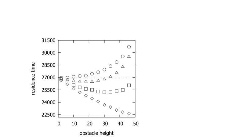
Figure 2.1: Residence time vs. obstacle height. The obstacle is placed at the center of the strip and its width is $W=2$ (disks). $W=20$ (triangles), $W=40$ (squares), and $W=60$ (diamonds). Simulation parameters: $L_{1}=200$, $L_{2}=50$, total number of inserted particles $5\cdot 10^{7}$. The total number of particles exiting through the right boundary decreases when the obstacle height is increased from $2.49\cdot 10^{5}$ (empty strip) to $1.69\cdot 10^{5}$ (disks), $0.99\cdot 10^{5}$ (triangles), and $0.68\cdot 10^{5}$ (squares) for $H=46$. The dashed line at $26930$ represents the value of the residence time measured for the empty strip.

In Figure 2.1 we report the residence time as a function of the obstacle height. The obstacle is placed at the center of the strip and its width is $W=2$ (disks), $W=20$ (triangles), $W=40$ (squares), and $W=60$ (diamonds). In the case of a thin barrier, starting from the empty strip value, the residence time increases with the height of the obstacle. For a wider obstacle, an a priori not intuitive result is found: the dependence of the residence time on the obstacle height is not monotonic. In the case $W=20$, starting from the empty strip value, the residence time decreases up to height $20$ and then increases to values above the empty strip one. This effect is even stronger if the width of the obstacle is further increased.

                                

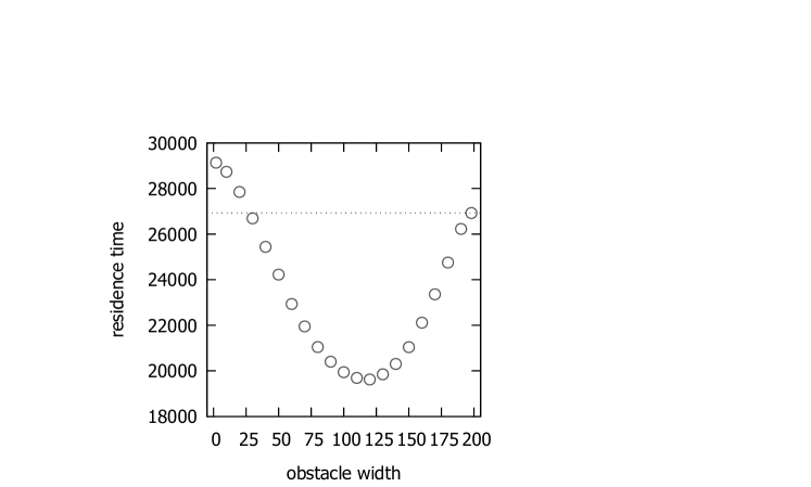
Figure 2.2: Residence time vs. obstacle width. The obstacle is placed at the center of the strip and its height is $H=40$. The total number of particles exiting through the right boundary decreases when the obstacle width is increased from $2\cdot 10^{5}$ for $W=2$ to $0.5\cdot 10^{5}$ for $W=198$. The parameters of the simulation and the dashed line are as in Figure 2.1.

In Figure 2.2 we plot the residence time as a function of the obstacle width. The obstacle is placed at the center of the strip and its height is $H=40$. When the barrier is thin the residence time is larger than the one measured in the empty strip case, but, when the width is increased, the residence time decreases and at about $26$ it becomes smaller than the empty case value. The minimum is reached at about $120$ (recall that the length of the strip is $L_{1}=200$ in this simulation), then the residence time increases to the empty strip value which is reached when the obstacle is as long as the entire strip. This is intuitively obvious, since in such a case the lattice consists of two independent channels having the same length as the original strip.

                                

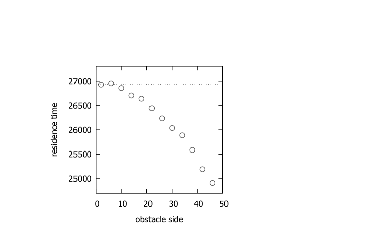
Figure 2.3: Residence time vs. squared obstacle side length. The squared obstacle is placed in the middle of the strip. The total number of particles exiting through the right boundary decreases when the obstacle side length is increased from $2.49\cdot 10^{5}$ (empty strip) to $0.63\cdot 10^{5}$ for side length equal to $46$. The parameters of the simulation and the dashed line are as in Figure 2.1.

In Figure 2.3 a centered square obstacle is considered. The residence time as a function of its side length is reported. Although small oscillations, reasonably due to numerical approximations, are visible, the behavior appears to be monotonically decreasing.

                                

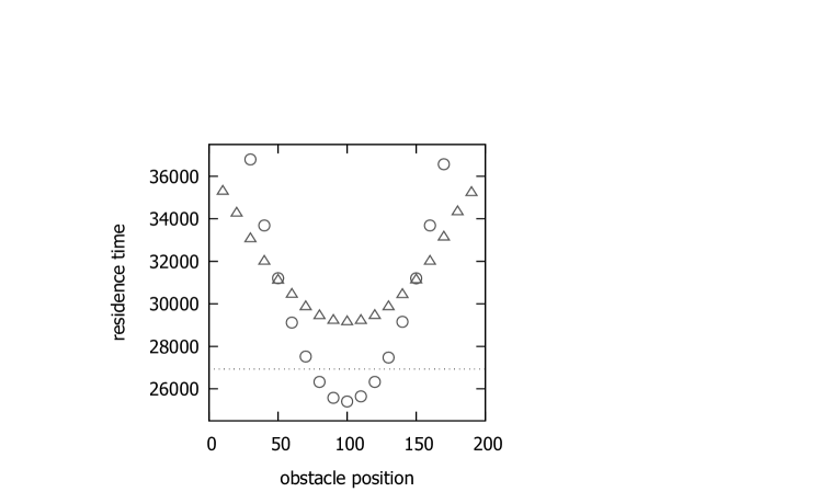
Figure 2.4: Residence time vs. position of the center of the obstacle. Disks refer to a squared obstacle with side length $40$, whereas triangles refers to a rectangular obstacle with width $W=2$ and height $H=40$. The total number of particles exiting through the right boundary is approximately $1.24\cdot 10^{5}$ (disks) and $2.01\cdot 10^{5}$ (triangles) and depends poorly on the obstacle position. The parameters of the simulation and the dashed line are as in Figure 2.1.

Finally, in Figure 2.4 we show that, and this is really surprising, the residence time is not monotonic even as a function of the position of the center of the obstacle. Disks refer to a squared obstacle of side length $40$, whereas triangles refer to a thin rectangular obstacle with width $W=2$ and height $H=40$. In both cases the residence time is not monotonic and attains its minimum value when the obstacle is placed in the center of the strip. In the squared obstacle case, when the abscissa of the center of the obstacle lies between $75$ and $125$ the residence time in presence of the obstacles is smaller than the corresponding value for the empty strip. On the other hand, for the thin rectangular obstacle, even if the non–monotonic behavior is found, the residence time is always larger than in the empty strip case. This fact is consistent with the results plotted in Figure 2.1.

The results that we found in the numerical experiments reported in Figures 2.1–2.4 can be summarized as follows: the residence time strongly depends on the obstacle geometry and position. In particular it seems that large centered obstacles favor the selection of particles crossing the strip faster than in the empty strip case.

In order to explain our observations, following [26], we partition the strip into three parts: the rectangular region on the left of the obstacle, the rectangular region on the right of the obstacle and the remaining central part containing the obstacle. As we will see later, the residence time behavior is consequence of two effects in competition: the total time spent by the particles in the channels between the obstacle and the horizontal boundary is smaller than the total time spent in the central part of the strip in the empty case. On the contrary, the total time spent both in the left and in the right part of the strip is larger with respect to the empty case. Both these two effects can be explained remarking that, when the obstacle is present, it is more difficult for the walker to enter the central region of the strip, namely, one of the channels flanking the obstacle. The total residence time trend depends on which of the two effects dominates the dynamics of the walker.

                      

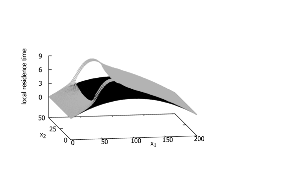
Figure 2.5: Mean time spent by the walker crossing the strip in each site of the strip (local residence time) for the empty strip case (black) and in presence of the obstacle (gray). Data are those of the experiment described by the disks in Figure 2.4. The obstacle is a squared obstacles with side length $40$ placed at the site with abscissa $60$.

To illustrate our interpretation of the phenomenon we describe in detail the walker behavior referring to the experiment associated with the disks in Figure 2.4. In Figure 2.5 we plot the mean time spent by the walker crossing the strip in each site of the strip. This quantity will be addressed as the local residence time. The gray surface in the picture refers to the obstacle case, whereas the black surface is related to the empty strip case. The data in the picture have been collected in the case in which the center of a squared obstacle with side length $40$ is placed at the site with coordinates $(80,25)$. The graph shows that in average in each site of the strip the particle spends a time larger than the time it spends at the same site in the empty strip case. This seems to be in contrast with the fact that the (total) residence time in the strip can be smaller when the obstacle is present. Indeed, this can happen since the sites of the strip falling in the obstacle region are never visited by the walker. It can then happen that the sum of the local residence times associated with sites in the central part of the strip in presence of the obstacle is smaller than the same sum computed in the empty strip case.

                                

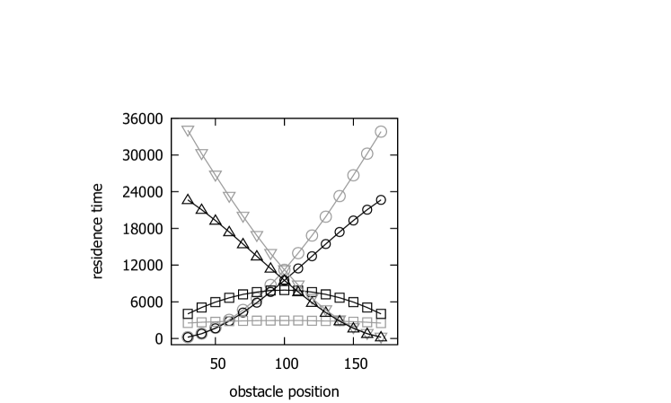
Figure 2.6: Total residence time in the left (circles), central (squares), and right (triangles) part of the strip in presence of the obstacle (gray) and in the empty strip case (black). The experiment associated with the disks in Figure 2.4 is considered.

Results in Figure 2.5 can be interpreted as follows. The local residence times in the left and in the right regions are larger with respect to the empty case since for the particle it is more difficult to access the central region and, thus, it will spend more time in the lateral parts of the strip. On the other hand, once the particle enters into one of the two central channels, it will take in average the same time to get back to one of the two lateral parts of the strip that it would take in absence of the obstacle. But, since, the number of the available sites in the central part is smaller when the obstacle is present, the local residence time will be larger.

The Figure 2.5 gives some new insight in the motion of the walker, but it is not sufficient to explain the residence time behavior discussed above. In order to get some insight into this, we compute the respective times spent by the particle in the left, central and right region of the strip. This is done in Figure 2.6, where data referring to the experiment associated with the disks in Figure 2.4 are reported. First, one should note that the total residence time in the left and in the right part of the strip are increased when the obstacle is present, this is due to the fact that for the particle it is more difficult to enter the central part when the obstacle is present. Moreover, precisely for the same reason the trajectory of the walker from its starting point to its exit from the strip will visit the channels in the central region of the strip a number of time smaller than the number of times that the particle visits the central region of the strip in the empty strip case. Thus, the residence time in the central part of the strip results to be smaller when the obstacle is present.

Hence, the behavior of the (total) residence time data reported as disks in Figure 2.4 can be explained as follows: if the center of the obstacle is close to the left boundary (say its abscissa is smaller than $75$) the effect in the right region of the strip dominates the one in the central region and the (total) residence time is increased (the effect in the left region in this case is negligible). On the other hand, if the center of the obstacle is close to the center of the strip (say its abscissa is between $75$ and $125$) the effect in the central region dominates and the (total) residence time is decreased. Finally, if the center of the obstacle is close to the right boundary (say its abscissa is larger than $125$) the effect in the left region of the strip dominates the one in the central region and the (total) residence time is increased (the effect in the right region in this case is negligible).

The behavior of the residence time in connection with all the experiments illustrated in Figures 2.1–2.4 can be explained similarly.

III The 1D model

In this section we propose a one–dimensional reduction of the problem based on a symmetric simple random walk with two defect sites. We actually prove that the behaviors of the 1D system are similar to those discussed above and that the Monte Carlo data are fully supported by exact analytical computations.

We consider a simple random walk on $\{0,1,\dots,L\}$. The sites $0$ and $L$ are absorbing, so that when the particle reaches one of these two sites the walk is stopped. All the sites $1,\dots,L-1$ are regular excepted for two sites called defect or special sites. The first or left defect site is the site $n+1$ and the second or right defect site is the site $n+h+2$, with $n=1,2,\dots,L-5$ and $h=1,2,\dots,L-n-4$. The parameters $n$ and $h$ are chosen in such a way that the left defect site cannot be $1$, the right defect site cannot be $L-1$, and there is at least one regular site separating the two defect sites. The number of regular sites on the left of the left defect site is $n$ and the number of regular sites in the region between the two defect sites is $h$. We let $w=L-(n+h+3)$ be the number of regular sites on the right of the right defect site.

At each unit of time the walker jumps to a neighbouring site according to the following rule: if it is on a regular site, then it performs a simple symmetric random walk. If it is at the left defect site it jumps with probability $\lambda$ to the right, with probability $1-\lambda-\epsilon$ to the left, and with probability $\epsilon$ it does not move. If it is at the right defect site it jumps with probability $\lambda$ to the left, with probability $1-\lambda-\epsilon$ to the right, and with probability $\epsilon$ it does not move. Here, $\lambda\in(0,1)$ and $\epsilon\in[0,1)$.

The array $1,\dots,L-1$ will be called the lane. The sites $0$ and $L$ will be, respectively, called the left and right exit of the lane.

This 1D model is a toy model for the 2D system that we have discussed in Section II. Indeed, the left defect site $n+1$ mimics the sites in the first column of the 2D strip on the left of the obstacle: the 2D walker in such a column has a probability to move to the right smaller than the probability to move to the left. Similarly, the right defect site $n+h+1$ mimics the sites in the first column to the right of the obstacle. Let us stress that the sites $n+1+1,\dots,n+h$ are regular, since when the 2D walker enters one of the two channels flanking the obstacle its probability to move to the right is equal to that to move to the left.

In this framework the residence time is defined by starting the walk at site $1$ and computing the typical time that the particle takes to reach the site $L$ provided the walker reaches $L$ before $0$. More precisely, we let $x_{t}$ be the position of the walker at time $t$ and denote by $\mathbb{P}_{k}$ and $\mathbb{E}_{k}$ the probability associated to the trajectories of the walk and the related average operator for the walk started at $x_{0}=k$ with $k=1,\dots,L-1$. We let

$$T_{i}=\inf\{t>0,\,x_{t}=i\}$$ (3.1)

be the first hitting time to $i$, with the convention that $T_{i}=\infty$ if the set $\{t>0,\,x_{t}=i\}$ is empty, i.e., the trajectory does not reach the site $i$. The main quantity of interest is the residence time or total residence time

$$R=\mathbb{E}_{1}[T_{L}|T_{L}<T_{0}]=\sum_{t=1}^{\infty}t\mathbb{P}_{1}[T_{L}=t|T_{L}<T_{0}]\;\;.$$ (3.2)

Note that the residence time is defined for the walk started at $x_{0}=1$ and the average is computed conditioning to the event $T_{L}<T_{0}$, namely, conditioning to the fact that the particle exits the lane through the right exit.

As in the 2D case discussed in Section II, we shall compute numerically the residence time by simulating many particles and averaging the time that each of them takes to exit through the right ending point, discarding all the particles exiting through the left ending point. But we stress that in this 1D model it is also possible to compute exactly the residence time. In this section we shall discuss our findings and in each plot the solid lines will represent the exact result which will be discussed in the following Section IV.

We now discuss our results for different choices of the parameter which are the analog of the cases considered in Section II for the 2D model. All the details about the numerical simulations are in the figure captions. The statistical error, since negligible, is not reported in the picture. We carry out the simulations with the following choice of the parameters:

$$\epsilon=\frac{1}{2}p\;\;\textrm{ and }\;\;\lambda=\frac{1}{2}(1-p)$$ (3.3)

with $p\in[0,1)$, so that $\epsilon\in[0,1/2)$ and $\lambda\in(0,1/2]$. Note that with such a choice the probability to move left (resp. right) for the particle sitting at the left (resp. right) defect site is $1-\lambda-\epsilon=1/2$. Note that for $p$ equal zero we recover the symmetric simple random walk, which mimics the 2D empty strip.

                                

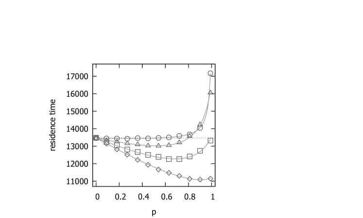
Figure 3.7: Residence time vs. $p$. Simulation parameters: total number of inserted particles $5\cdot 10^{7}$, $L=201$, $n=98$ and $h=2$ (disks), $n=89$ and $h=20$ (triangles), $n=79$ and $h=40$ (squares), and $n=69$ and $h=60$ (diamonds). The total number of particles exiting through the right exit decreases when $p$ grows from $2.48\cdot 10^{5}$ (no defect is present, namely, $p=0$) to $1\cdot 10^{5}$ (disks), $0.22\cdot 10^{5}$ (triangles), $0.12\cdot 10^{5}$ (squares), and $0.08\cdot 10^{5}$ (diamonds) for $p=0.99$. The dashed line at $13466$ line represents the value of the residence time measured in absence of defect sites ($p=0$). The solid line is the exact solution.

The case reported in Figure 3.7 is the analog of the case discussed in Figure 2.1 in the 2D setting. Indeed, the residence time is plotted as a function of the parameter $p$ increasing from $0$ to $0.99$ and this mimics the increase of the height of the obstacle considered in Figure 2.1. Moreover, the two defect sites are symmetric with respect to the middle point of the lane and the number of regular sites between them is chosen equal to $2$, $20$, $40$, and $60$ mimicking the different obstacle widths considered in Figure 2.1. The data show a behavior similar to that reported in Figure 2.1 in the 2D case: in the case $h=2$ (the defect sites are close to each other) the residence time increases with $p$. For a wider obstacle, the non–monotonic behavior is recovered. In the case $h=20$, starting from the empty strip value, the residence time decreases up to $p\sim 0.55$ and then it increases to values above the $p=0$ case. This effect is even stronger if $p$ is further increased.

                                

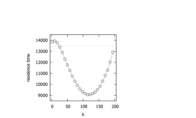
Figure 3.8: Residence time vs. $h$ (even) for $p=0.84$, $L=201$, $n=(L-h-3)/2$, and total number of inserted particles $5\cdot 10^{7}$. The dashed and the solid lines are as in Figure 3.7. The total number of particles exiting through the right exit decreases when $h$ is increased from $2.31\cdot 10^{5}$ for $h=2$ to $0.41\cdot 10^{5}$ for $h=194$.

The case reported in Figure 3.8 is the analog of the case discussed in Figure 2.2 in the 2D setting. Indeed, the residence time is plotted as a function of the parameter $h$ increasing from $2$ to $198$ with the two defect sites symmetric with respect to the middle point of the lane. This case mimics the increase of the width of the centered rectangular obstacle reported in Figure 2.2. When $h$ is small the residence time is larger than the one measured for $p=0$, but, when $h$ is increased, the residence time decreases and at about $25$ it becomes smaller than the $p=0$ case. The minimum is reached at about $120$ (recall the lane is long $201$ sites in this simulation), then the residence time increases towards the $p=0$ value.

                                

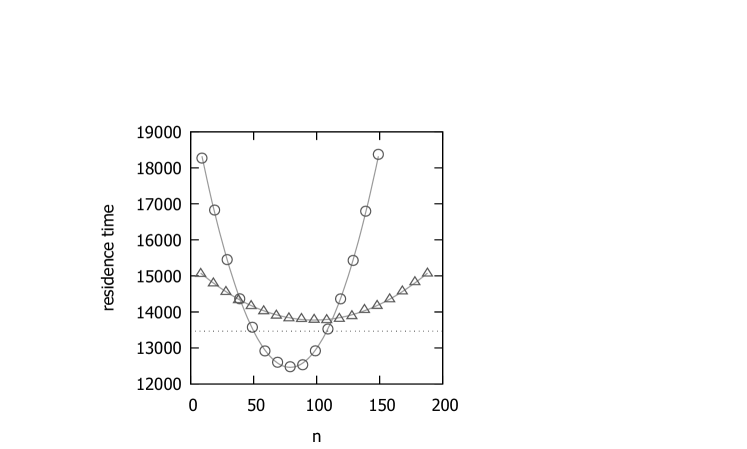
Figure 3.9: Residence time vs. $n$ for $p=0.84$, $L=201$, $h=40$ (disks), $h=2$ (triangles), and total number of inserted particles $5\cdot 10^{7}$. The dashed and the solid lines are as in Figure 3.7. The total number of particles exiting through the right exit is approximately equal to $1.2\cdot 10^{5}$ (disks) and $2.3\cdot 10^{5}$ (triangles).

In this 1D setting it is not really clear how to construct an analog for the experiment in Figure 2.3, where a squared centered obstacle was considered. On the other hand, the case reported in Figure 3.9 is the analog of the case discussed in Figure 2.4 in the 2D setting. Indeed, the residence time is plotted as a function of the parameter $n$ in the two cases $h=40$ (disks) and $h=2$ (triangles). This case mimics the increase of the abscissa of the center of the obstacle reported in Figure 2.4. In both cases the residence time is non–monotonic and attains its minimum value when the defect sites are symmetric with respect to the center of the lane. In the $h=40$ case, when $n$ lies approximately between $50$ and $110$ the residence time is smaller than the corresponding value for the case $p=0$. On the other hand, for $h=2$, even if the non–monotonic behavior is recovered, the residence time is always larger than the one measured in the $p=0$ case. This fact is consistent with the results plotted in Figure 3.7.

                                

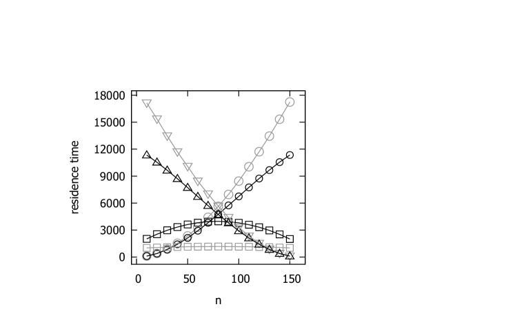
Figure 3.10: Total residence time in the left (circles), central (squares), and right (triangles) region of the lane in presence of the defect sites (gray) and in the $p=0$ case (black). The experiment associated with the disks in Figure 3.9 is considered.

In order to explain these observations, similarly to what we did in the 2D case and in [26], we partition the lane into three parts: the part of the lane on the left of the left defect (left region), the part of the lane between the two defect sites (central region), and the part of the lane on the right of the right defect (right region). As in the 2D case, the residence time behavior is consequence of two effects in competition: the total time spent by the particles in the central region is smaller than the total time spent in the same region in absence of defect sites ($p=0$). On the contrary, the total time spent both in the left and in the right region is larger with respect to the time spent there in the $p=0$ case. Both these two effects can be explained remarking that, in presence of defect sites, it is more difficult for the walker to enter the central region of the lane. The total residence time trend depends on which of the two effects dominates the dynamics of the walker.

These remarks are illustrated in Figure 3.10, data referring to the experiment associated with the disks in Figure 3.9 are reported. Again, one notes that the total residence time in the left and in the right regions of the lane are increased when the defect sites are present, this is due to the fact that for the particle it is more difficult to enter the central region in such a case. Moreover, precisely for the same reason the trajectory of the walker from its starting point $1$ to its exit from the lane will visit the central region of the lane a number of time smaller than the number of times that the particle visits such a region in the $p=0$ case. Thus, the residence time in the central region results to be smaller in presence of the defect site. Finally, similarly to what we did in the 2D case, the results in Figure 3.10 allows a complete interpretation of the residence time behavior depicted by the disks in Figure 3.9 (note that the maximum value of the variable $n$ for the disks in Figure 3.9 is $150$).

IV Analytic results

In this section we derive exact, though not explicit, expressions for the residence time defined in Section III. To compute the residence time, we shall make use of the following result on a five state chain: the states are $S$, $A$, $B$, $C$, and $D$. The jump probabilities are as depicted in the figure 4.11 and the chain is started at time $0$ in $B$. We prove that the probability $Q_{k}$, with $k\geq 1$, for the chain to reach $D$ before $S$ and return $k-1$ times to the site $B$ before reaching $D$ is

$$Q_{k}=p_{B}p_{C}[r_{B}+q_{B}p_{A}+p_{B}q_{C}]^{k-1}\;\;,$$ (4.4)

where $r_{B}=1-(p_{B}+q_{B})$. Indeed,

$$\begin{split}Q_{k}&=p_{B}p_{C}\sum_{r=0}^{k-1}{{k-1}\choose{r}}(p_{B}q_{C})^{k-1-r}\\ &\phantom{mmmmmmmm}\times\sum_{s=0}^{r}{{r}\choose{s}}(q_{B}p_{A})^{s}(r_{B})^{r-s}\end{split}$$

where $r$ counts the number of times that, starting from $B$, the chain either jumps to $A$ or it stays in $B$ and $s$ counts the number of times that starting from $B$ it jumps to $A$. The equation (4.4) is then proven by using the binomial theorem.

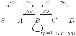
Figure 4.11: Schematic representation of the five state chain model.

We now consider again to the 1D walk defined in Section III. To compute the residence time we introduce the local times, i.e., the time spent by a trajectory at site $i$ defined as

$$\tau_{i}=|\{t>0,x_{t}=i\}|$$ (4.5)

for any $i=1,\dots,L-1$, where $|A|$ denotes the cardinality of the set $A$. Provided $T_{L}$ is finite, we have that

$$T_{L}=\sum_{i=1}^{L-1}\tau_{i}\;\;.$$ (4.6)

Hence the residence time $R$ defined in (3.2) can be expressed as

$$R=\sum_{i=1}^{L-1}\mathbb{E}_{1}[\tau_{i}|T_{L}<T_{0}]$$ (4.7)

and for all $i\in\{1,\ldots,L-1\}$

$$\begin{split}&\mathbb{E}_{1}[\tau_{i}|T_{L}<T_{0}]\vphantom{\bigg{\{}}\\ &\phantom{m}=\frac{\mathbb{P}_{1}[T_{i}<T_{0}]}{\mathbb{P}_{1}[T_{L}<T_{0}]}\frac{p_{B}p_{C}}{[1-(r_{B}+q_{B}p_{A}+p_{B}q_{C})]^{2}}\;\;,\end{split}$$ (4.8)

where we defined the quantities

$$\begin{array}[]{ll}p_{A}=\mathbb{P}_{i-1}(T_{i}<T_{0}),&q_{A}=\mathbb{P}_{i-1}(T_{0}<T_{i}),\\ p_{B}=\mathbb{P}_{i}(x_{1}=i+1),&q_{B}=\mathbb{P}_{i}(x_{1}=i-1),\\ p_{C}=\mathbb{P}_{i+1}(T_{L}<T_{i}),&q_{C}=\mathbb{P}_{i+1}(T_{i}<T_{L}).\end{array}$$ (4.9)

Note that $p_{A}+q_{A}=1$, $p_{B}+q_{B}+r_{B}=1$, and $p_{C}+q_{C}=1$. Indeed, we have

$$\mathbb{E}_{1}[\tau_{i}|T_{L}<T_{0}]=\sum_{k=1}^{\infty}k\mathbb{P}_{1}[\{i\textrm{ visited }k\textrm{ times}\}|\{T_{L}<T_{0}\}]$$

and, using the definition of conditional probability and the Markov property,

$$\begin{split}&\mathbb{E}_{1}[\tau_{i}|T_{L}<T_{0}]\\ &\phantom{m}=\sum_{k=1}^{\infty}k(\mathbb{P}_{1}[\{T_{i}<T_{0}\}]/\mathbb{P}_{1}[\{T_{L}<T_{0}\}])\\ &\phantom{mmmmm}\times\mathbb{P}_{i}[\{T_{L}<T_{0}\}\cap\{k-1\textrm{ returns to }i\}]\;.\end{split}$$

The last probability appearing in the above expression is nothing but the quantity $Q_{k}$ defined for the five state chain with the jump probabilities defined as in (4.9). Finally, (4.8) follows by noting that

$$\sum_{k=1}^{\infty}kQ_{k}=\frac{p_{B}p_{C}}{[1-(r_{B}+q_{B}p_{A}+p_{B}q_{C})]^{2}}\;\;.$$

Our strategy to compute the residence time is the following: for any $i=1,\dots,L-1$ we shall compute $\mathbb{E}_{1}[\tau_{i}|T_{L}<T_{0}]$ identifying the correct values of $p_{A}$, $q_{A}$, $p_{B}$, $q_{B}$, $p_{C}$, and $q_{C}$ to be used, whose definition depends on the choice of the site $i$. Finally, the sum (4.7) will provide us with the residence time.

IV.1 Residence time in the symmetric case

In the symmetric case, that is $\epsilon=0$ and $\lambda=1/2$, by using the gambler’s ruin result we have that

$$\mathbb{P}_{1}[T_{0}<T_{L}]=\frac{L-1}{L}$$ (4.10)

and

$$\mathbb{P}_{1}[T_{L}<T_{0}]=\frac{1}{L}\;\;.$$ (4.11)

This is a very classical problem in probability theory which can be found in any probability text book, see, for example, [27, paragraphs 2 and 3, Chapter XIV].

                                

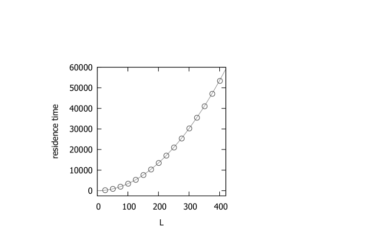
Figure 4.12: Residence time vs. $L$ for the lane with no singular sites (symmetric case). The solid line is the exact solution (4.12), whereas circles are the average results of a Monte Carlo simulation with $5\cdot 10^{8}$ particles started at the site $1$.

The computation of the residence time, which, in the gambler language, is the average duration of the game conditioned to the fact that the gambler wins, is not immediate. We use the formulas (4.7)–(4.9) proven above by defining suitably the five state chain jump probabilities. More precisely, $p_{A}=(i-1)/i$ is given by (4.10) with the initial point $1$ replaced by $i-1$ and $L$ replaced by $i$, $q_{A}=1/i$ is similarly given by (4.11), $p_{B}=q_{B}=1/2$ (and hence $r_{B}=0$), $p_{C}=1/(L-i)$ is given by (4.11) with the initial point $1$ replaced by $i+1$ and $L$ replaced by $L-i$, and $q_{C}=(L-i-1)/(L-i)$ is given similarly by (4.10). Moreover, since from (4.10) it also follows that $\mathbb{P}_{1}[T_{L}<T_{0}]=1/L$ and $\mathbb{P}_{1}[T_{i}<T_{0}]=1/i$, from (4.8) a straightforward computation yields

$$\mathbb{E}_{1}[\tau_{i}|T_{L}<T_{0}]=\frac{2}{L}(Li-i^{2})$$

and, computing the sum in (4.7), we finally have

$$R=\frac{1}{3}(L-1)(L+1)\;\;.$$ (4.12)

In figure 4.12 the numerical estimate of the residence time in this symmetric case is compared to the exact result (4.12). It is interesting to remark that the mean time that a symmetric walk started at $0$ needs to reach either $-L$ or $+L$ is $L^{2}$. This time can be computed as the average duration of the gambler’s game. Thus, conditioning the particle to exit through the right end point decreases by a multiplicative factor the mean time that the particle needs to reach the distance $L$ from the starting point, but it does not change the diffusive dependence on the length $L$ of the lane.

IV.2 Crossing probability in the general case

We now come back to the general 1D model introduced in Section III. As a first step in the residence time computation, we have to calculate the crossing probability $\mathbb{P}_{1}[T_{L}<T_{0}]$ which appears at the denominator in (4.8). We first note that, by using repeatedly the Markov property, one gets

$$\mathbb{P}_{1}[T_{0}<T_{L}]=1-p_{1}p_{2}p_{3}p_{4}p_{5}$$ (4.13)

and, as a consequence

$$\mathbb{P}_{1}[T_{L}<T_{0}]=p_{1}p_{2}p_{3}p_{4}p_{5}$$ (4.14)

where

$$\begin{split}&p_{1}=\mathbb{P}_{1}[T_{0}>T_{n+1}],\;p_{2}=\mathbb{P}_{n+1}[T_{0}>T_{n+2}],\;\\ &p_{3}=\mathbb{P}_{n+2}[T_{0}>T_{n+h+2}],\;p_{4}=\mathbb{P}_{n+h+2}[T_{0}>T_{n+h+3}],\;\\ &p_{5}=\mathbb{P}_{n+h+3}[T_{0}>T_{L}].\end{split}$$

The probabilities $p_{1},\dots,p_{5}$ can be computed explicitly and the remaining part of this section is devoted to the computation of these quantities. For $p_{1}$ one has to use (4.11) with $L$ replaced by $n+1$ to deduce that

$$p_{1}=\frac{1}{n+1}\;\;.$$ (4.15)

To compute $p_{2}$, we first note that, once the particle is in $n$, the probability to come back to $n+1$ before reaching $0$ is equal to $n/(n+1)$, as it follows by using (4.10) with the initial point $1$ replaced by $n$ and $L$ replaced by $n+1$. Hence,

$$p_{2}=\sum_{r=0}^{\infty}\sum_{k=0}^{r}{{r}\choose{k}}\Big{[}(1-\varepsilon-\lambda)\frac{n}{n+1}\Big{]}^{r-k}\varepsilon^{k}\lambda$$

where $r$ counts the number of times that, starting from $n+1$, the walker either jumps to $n$ or it stays in $n+1$ and $k$ counts the number of times that the walker stays in $n+1$. Using the binomial theorem, we get

$$p_{2}=\frac{\lambda}{1-[(1-\varepsilon-\lambda)n/(n+1)+\varepsilon]}\;.$$ (4.16)

In order to compute $p_{3}$, note that, using (4.10) and (4.11) with initial point $n+2$ and replacing $L$ with $h+1$, one has $\mathbb{P}_{n+2}[T_{n+1}<T_{n+h+2}]=h/(h+1)$ and $\mathbb{P}_{n+2}[T_{n+h+2}<T_{n+1}]=1/(h+1)$. Hence,

$$p_{3}=\frac{1}{h+1}\sum_{k=0}^{\infty}\Big{(}\frac{h}{h+1}\Big{)}^{k}p_{2}^{k}=\frac{1}{1+h(1-p_{2})}\;,$$ (4.17)

where $k$ counts the number of times that, starting from $n+2$, the walker reaches $n+1$ before $n+h+2$.

To compute $p_{4}$, we first need to calculate $\xi=\mathbb{P}_{n+h+1}[T_{0}>T_{n+h+2}]$. Starting from $n+h+1$ the probability to reach $n+h+2$ before $n+1$ is $\mathbb{P}_{n+h+1}[T_{n+h+2}<T_{n+1}]=h/(h+1)$, where we used (4.10) with initial point $n+h+1$ and $L$ replaced by $h+1$. Hence, $\mathbb{P}_{n+h+1}[T_{n+1}<T_{n+h+2}]=1/(h+1)$. Thus,

$$\xi=\frac{h}{h+1}+\frac{1}{h+1}p_{2}\frac{1}{h+1}\sum_{k=0}^{\infty}\Big{(}p_{2}\frac{h}{h+1}\Big{)}^{k}$$

where $k$ counts the number of times that the walker returns to $n+1$ after having visited it for the first time. We have also used that $\mathbb{P}_{n+2}[T_{n+1}<T_{n+h+2}]=h/(h+1)$. With some algebra we find the expression

$$\xi=\frac{p_{2}+h(1-p_{2})}{1+h(1-p_{2})}\;\;.$$ (4.18)

Now, we have all the ingredients to compute $p_{4}$. Indeed,

$$p_{4}=(1-\varepsilon-\lambda)\Big{[}\sum_{r=0}^{\infty}\sum_{k=0}^{r}{{r}\choose{k}}\varepsilon^{k}(\lambda\xi)^{r-k}\Big{]}$$

where $r-k$ counts the number of times that the walker starting from $n+h+2$ jumps to $n+h+1$ and where $k$ counts the number of times that the walker stays at $n+h+2$. A simple calculation provides the result

$$p_{4}=\frac{1-\varepsilon-\lambda}{1-(\lambda\xi+\varepsilon)}\;\;.$$ (4.19)

Finally, to compute $p_{5}$ we remark that $\mathbb{P}_{n+h+3}[T_{L}<T_{n+h+2}]=1/(w+1)$ and $\mathbb{P}_{n+h+3}[T_{n+h+2}<T_{L}]=w/(w+1)$, as it can be deduced by (4.11) and (4.10) by using as initial point the point $n+h+3$ and replacing $L$ by $w+1$. Then,

$$p_{5}=\frac{1}{w+1}\sum_{k=0}^{\infty}\Big{(}\frac{w}{w+1}p_{4}\Big{)}^{k}=\frac{1}{1+w(1-p_{4})}\;\;.$$ (4.20)

Finally, plugging the equations (4.15)–(4.20) in (4.14), we find the expression

$$\mathbb{P}_{1}[T_{L}<T_{0}]=\frac{\lambda}{(1+h)(1-\varepsilon-2\lambda)+\lambda L}$$ (4.21)

for the probability that the particle started at the site $1$ reaches $L$ before visiting $0$. It is interesting to remark that in the case $\varepsilon=0$ and $\lambda=1/2$ the expression (4.11) valid in the symmetric case is recovered.

IV.3 Residence time in presence of defects

The last step, necessary to complete our algorithm to compute the residence time, is that of listing the expression that must be used for the probabilities (4.9) for the different choices of $i$ on the lattice. In this last section, in order to get simpler formulas, we focus on the case that has been studied numerically, that is to say, we choose the parameterization (3.3). First of all we note that the expression (4.21) of the probability that the particle started at the site $1$ reaches $L$ before visiting $0$ simplifies to

$$\mathbb{P}_{1}[T_{L}<T_{0}]=\frac{1-p}{p(1+h)+(1-p)L}\;\;.$$ (4.22)

The site $i$ in the lattice can be chosen in nine possible different ways: in the bulk of the three regions on the left, between and on the right of the defect sites, as one of the four sites neighboring the defects and as one of the two defect site. We list only five cases, the remaining four can be deduced exchanging the role of the parameters $n$ and $w$. Note that we shall only list either $p_{A}$ or $q_{A}$ and $p_{C}$ or $q_{C}$; the missing parameter can be deduced by the equations $p_{A}+q_{A}=1$ and $p_{C}+q_{C}=1$.

Case $1\leq i\leq n-1$. First note that $\mathbb{P}_{1}[T_{i}<T_{0}]=1/i$ is given by (4.11) with initial site $1$ and $L$ replaced by $i$. Moreover, $p_{A}=(i-1)/i$ follows from (4.10) with initial site $i-1$ and $L$ replaced by $i$. We trivially have that $p_{B}=q_{B}=1/2$. Finally, $p_{C}=(1-p)/[p(1+h)+(1-p)(L-i)]$ follows from (4.22) with initial site $i+1$ and $L$ replaced by $L-i$.

Case $i=n$. First note that $\mathbb{P}_{1}[T_{i}<T_{0}]=1/n$ is given by (4.11) with initial site $1$ and $L$ replaced by $n$. Moreover, $p_{A}=(n-1)/n$ follows from (4.10) with initial site $n-1$ and $L$ replaced by $n$. We trivially have that $p_{B}=q_{B}=1/2$. Finally, we note that $q_{C}$ has the same structure as $p_{4}$, thus, by exchanging the role of $n$ and $w$, from (4.16), (4.18), and (4.20) we have that $q_{C}=1/[2-p-(1-p)\zeta]$ where

$$\zeta=\frac{\pi+h(1-\pi)}{1+h(1-\pi)}\;\textrm{ and }\;\pi=\frac{1-p}{2-p-\frac{w}{w+1}}\;.$$ (4.23)

Case $i=n+1$. First note that $\mathbb{P}_{1}[T_{i}<T_{0}]=1/(n+1)$ is given by (4.11) with initial site $1$ and $L$ replaced by $n+1$. Moreover, $p_{A}=n/(n+1)$ follows from (4.10) with initial site $n$ and $L$ replaced by $n$. We trivially have that $p_{B}=(1-p)/2$ and $q_{B}=1/2$. Finally, we note that $q_{C}$ has the same structure as $\xi$, thus, by exchanging the role of $n$ and $w$, from (4.18) we have that $q_{C}=\zeta$, see (4.23).

Case $i=n+2$. First note that $\mathbb{P}_{1}[T_{i}<T_{0}]=p_{1}p_{2}$, hence, using (4.15) and (4.16), an easy computation yields $\mathbb{P}_{1}[T_{i}<T_{0}]=(1-p)/[(n+1)(2-p-n/(n+1))]=(1-p)/(2+n-p(n+1))$ since, with the parameterization that we are adopting in this section

$$p_{2}=\frac{1-p}{2-p-n/(n+1)}\;\;.$$

Moreover, $p_{A}=p_{2}$ by definition and $p_{B}=q_{B}=1/2$. Finally, we note that $q_{C}$ has the same structure as $\xi$ with $h$ replaced by $h-1$. Thus, by exchanging the role of $n$ and $w$, from (4.18) we have that $q_{C}=[\pi+(h-1)(1-\pi)]/[1+(h-1)(1-\pi)]$, with $\pi$ defined in (4.23).

Case $n+3\leq i\leq n+h$. First note that $\mathbb{P}_{1}[T_{i}<T_{0}]=p_{1}p_{2}\bar{p}_{3}$, where $\bar{p}_{3}$ has the structure of $p_{3}$ with $h$ replaced by $i-(n+2)$. Hence (4.17) gives us $\mathbb{P}_{1}[T_{i}<T_{0}]=(p_{1}p_{2})/(1+(i-n-2)(1-p_{2}))$ with $p_{1}$ and $p_{2}$ as in the previous case. Moreover, $p_{A}$ has the same structure as $\xi$ with $h$ replaced by $i-n-2$ so $p_{A}=({p_{2}+(i-n-2)(1-p_{2})})/({1+(i-n-2)(1-p_{2})})$ and $p_{B}=q_{B}=1/2$. Finally, we note that $q_{C}$ has the same structure as $\xi$ with $h$ replaced by $n+h+1-i$. Thus, by exchanging the role of $n$ and $w$, from (4.18) we have that $q_{C}=[\pi+(n+h+1-i)(1-\pi)]/[1+(n+h+1-i)(1-\pi)]$, with $\pi$ defined in (4.23).

V Conclusions

We have studied in detail the effect of an obstacle in a 2D strip on the flux of particles performing a simple symmetric random walk. We have found that, due to purely geometrical effects, the typical time that a particle entered in strip through the left boundary and leaving the system through the right boundary has a complex dependence on the geometrical parameters of the obstacle. In particular, we stress that we found non–monotonic behaviors as a function of a sufficiently large obstacle. These phenomena have been interpreted in terms of the total time that the particles spend in each of the three regions of the strip in which the obstacle naturally partitions the lattice: the one on its left, the one on its right, and the channels between the obstacle and the horizontal boundary. Finally, we have studied numerically and analytically a 1D model mimicking the 2D random walk and we have found similar results. In this case we have been able to develop a complete analytical computation and to compare our numerical results to the exact solution.

- [1] E. Cristiani and D. Peri. Applied Mathematical Modelling, 45:285 – 302, 2017.
- [2] M.J. Saxton. Biophysical Journal, 66:394–401, Feb 1994.
- [3] F. Höfling and T. Franosch. Reports on Progress in Physics, 76(4), 2013.
- [4] M.A. Mourão, J.B. Hakim, and S. Schnell. Biophysical Journal, 107:2761–2766, Jun 2017.
- [5] A.J. Ellery, M.J. Simpson, S.W. McCue, and R.E. Baker. The Journal of Chemical Physics, 140(5):054108, 2014.
- [6] K. To, P. Lai, and H.K. Pak. Phys. Rev. Lett., 86:71–74, Jan 2001.
- [7] I. Zuriguel, A. Garcimartín, D. Maza, L.A. Pugnaloni, and J.M. Pastor. Phys. Rev. E, 71:051303, May 2005.
- [8] F. Alonso–Marroquin, S.I. Azeezullah, S.A. Galindo–Torres, and L.M. Olsen-Kettle. Phys. Rev. E, 85:020301, Feb 2012.
- [9] I. Zuriguel, A. Janda, A. Garcimartín, C. Lozano, R. Arévalo, and D. Maza. Phys. Rev. Lett., 107:278001, Dec 2011.
- [10] D. Helbing. Rev. Mod. Phys., 73:1067–1141, Dec 2001.
- [11] N. Bellomo and C. Dogbé. SIAM Review, 53(3):409–463, 2011.
- [12] D. Helbing, P. Molnár, I.J. Farkas, and K. Bolay. Environment and Planning B: Planning and Design, 28(3):361–383, 2001.
- [13] D. Helbing, I. Farkas, P. Molnàr, and T. Vicsek. In M. Schreckenberg and S. D. Sharma, editors, Pedestrian and Evacuation Dynamics, pages 21–58, Berlin, 2002. Springer.
- [14] E.N.M. Cirillo and A. Muntean. Physica A: Statistical Mechanics and its Applications, 392(17):3578 – 3588, 2013.
- [15] G. Albi, M. Bongini, E. Cristiani, and D. Kalise. SIAM Journal on Applied Mathematics, 76(4):1683–1710, 2016.
- [16] D. Helbing, I. Farkas, and T. Vicsek. Nature, 407:487–490, Sep 2000.
- [17] D. Helbing, L. Buzna, A. Johansson, and T. Werner. Transportation Science, 39(1):1–24, 2005.
- [18] R. Escobar and A. De La Rosa. In W. Banzhaf, J. Ziegler, T. Christaller, P. Dittrich, and J.T. Kim, editors, Advances in Artificial Life, Proceedings of hte 7th European COnference, ECAL, 2003, Dortmund, germany, September 14–17, 2003, Proceedings. Lecture Notes in Computer Science, vol. 2801., pages 97–106, Berlin, 2003. Springer.
- [19] A. Muntean, E.N.M. Cirillo, O. Krehel, M. Bohm, In “Collective Dynamics from Bacteria to Crowds”, An Excursion Through Modeling, Analysis and Simulation Series: CISM International Centre for Mechanical Sciences, Vol. 553 Muntean, Adrian, Toschi, Federico (Eds.) 2014, VII, 177 p. 29 illus, Springer, 2014.
- [20] E.N.M. Cirillo, A. Muntean, Comptes Rendus Macanique 340, 626–628, 2012
- [21] D. Braess, A. Nagurney, and T. Wakolbinger. Transportation Science, 39(4):446–450, 2005.
- [22] R.L. Hughes. Annual Review of Fluid Mechanics, 35:169–182, 2003.
- [23] E.N.M. Cirillo, O. Krehel, A. Muntean, and R. van Santen. Phys. Rev. E, 94:042115, Oct 2016.
- [24] E.N.M. Cirillo, O. Krehel, A. Muntean, R. van Santen, and Aditya S. Physica A: Statistical Mechanics and its Applications, 442:436 – 457, 2016.
- [25] B.W. Fitzgerald, J.T. Padding, and R. van Santen. Phys. Rev. E, 95:013307, Jan 2017.
- [26] A. Ciallella and E.N.M. Cirillo. Linear boltzmann dynamics in a strip with large reflective obstacles: stationary state and residence time. Preprint, arXiv:1707.09950, 2017.
- [27] W. Feller. An Introduction to Probability Theory and its Applications, volume 1. John wiley & Sons, Inc, New York – London – Sidney, 1968.