Abstract

We analyse for the first time the CP violating ratio $\varepsilon^{\prime}/\varepsilon$ in $K\to\pi\pi$ decays in leptoquark (LQ) models. Assuming a mass gap to the electroweak (EW) scale, the main mechanism for LQs to contribute to $\varepsilon^{\prime}/\varepsilon$ is EW gauge-mixing of semi-leptonic into non-leptonic operators, which we treat in the Standard Model effective theory (SMEFT). We perform also the one-loop decoupling for scalar LQs, finding that in all models with both left-handed and right-handed LQ couplings box-diagrams generate numerically strongly enhanced EW-penguin operators $Q_{8,8^{\prime}}$ already at the LQ scale. We then investigate correlations of $\varepsilon^{\prime}/\varepsilon$ with rare Kaon processes ($K_{L}\rightarrow\pi^{0}\nu\bar{\nu}$, $K^{+}\rightarrow\pi^{+}\nu\bar{\nu}$, $K_{L}\to\pi^{0}\ell\bar{\ell}$, $K_{S}\to\mu\bar{\mu}$, $\Delta M_{K}$ and $\varepsilon_{K}$) and find that even imposing only a moderate enhancement of $(\varepsilon^{\prime}/\varepsilon)_{\rm NP}=5\times 10^{-4}$ to explain the current anomaly hinted by the Dual QCD approach and RBC-UKQCD lattice QCD calculations leads to conflicts with experimental upper bounds on rare Kaon processes. They exclude all LQ models with only a single coupling as an explanation of the $\varepsilon^{\prime}/\varepsilon$ anomaly and put strong-to-serious constraints on parameter spaces of the remaining models. Future results on $K^{+}\rightarrow\pi^{+}\nu\bar{\nu}$ from the NA62 collaboration, $K_{L}\rightarrow\pi^{0}\nu\bar{\nu}$ from the KOTO experiment and $K_{S}\to\mu\bar{\mu}$ from LHCb will even stronger exhibit the difficulty of LQ models in explaining the measured $\varepsilon^{\prime}/\varepsilon$, in case the $\varepsilon^{\prime}/\varepsilon$ anomaly will be confirmed by improved lattice QCD calculations. Hopefully also improved measurements of $K_{L}\to\pi^{0}\ell\bar{\ell}$ decays will one day help in this context.

1 Introduction

Leptoquarks (LQs) are very special new particles as they couple directly quarks to leptons and consequently carry both baryon and lepton number, $B$ and $L$. Moreover, they are strongly interacting, carry fractional electric charges but in contrast to quarks they are bosons: either scalars or vectors [1, 2, 3, 4]. Because of these rather special properties of LQs the phenomenological implications of models containing them are markedly different than the ones where new scalars and gauge bosons couple directly only leptons to leptons and quarks to quarks.

Indeed quite generally the pattern of flavour violations within LQ models is as follows.

• The semi-leptonic and leptonic decays of mesons are privileged as in these models they can naturally appear already at tree-level. This applies in particular to many rare decays which are loop suppressed within the SM. Therefore, the presence of departures from SM expectations for such decays can naturally be explained in some LQ models.

• On the other hand all non-leptonic decays of mesons and also purely leptonic processes are loop-suppressed within LQ models.

• In consequence, large LQ effects in semi-leptonic and leptonic decays of mesons do not necessarily imply large modifications of SM predictions for non-leptonic observables for which the SM, with few notable exceptions discussed below, offers a good description of the data. On the other hand in view of a very strong suppression of FCNCs in purely leptonic processes within the SM, still large LQ effects in these processes can be found in spite of their loop suppression providing thereby strong constraints on LQ models.

• Moreover, it should be emphasized that in LQ models in which the only new particles are LQs, the fermions exchanged in the loops are leptons in non-leptonic meson decays but SM quarks in the case of purely leptonic processes. Thus these processes are sensitive to the sum over all LQ couplings of the particles in the loop.

Most flavour analyses of LQs in the literature concentrated on semi-leptonic decays of mesons, purely leptonic processes and $B^{0}_{s,d}-\bar{B}^{0}_{s,d}$ mixing. We refer to selected recent papers [5, 6, 7, 8, 9, 10] for further references to a very rich literature. In this context, the loop-suppression of LQ contributions to non-leptonic transitions is certainly useful for those non-leptonic observables for which the SM predictions agree well with data as strong constraints on LQ parameters from them can be avoided making the explanation of $B$ physics anomalies easier.

In the present paper we will address the ratio $\varepsilon^{\prime}/\varepsilon$ and its correlation with rare Kaon decays, which to our knowledge has never been studied in LQ models. This is motivated by the recent results on $\varepsilon^{\prime}/\varepsilon$ from lattice QCD [11, 12] and Dual QCD large $N$ approach [13, 14] that have shown the emerging anomaly in $\varepsilon^{\prime}/\varepsilon$ [15] with its value in the SM being significantly below the experimental world average from NA48 [16] and KTeV [17, 18] collaborations. This finding has been confirmed in [19]. We will assume a mass gap between the new physics scale of the order of the LQ mass ${\mu_{\Lambda}}\sim M_{\rm LQ}$ and the electroweak (EW) scale ${\mu_{\rm ew}}$, which is conveniently done in the framework of Standard Model effective theory (SMEFT). In our analysis of LQ models we will assume nonvanishing contributions to $\varepsilon^{\prime}/\varepsilon$ to explain the anomaly, and find that it would automatically imply too large deviations in $K_{L}\rightarrow\pi^{0}\nu\bar{\nu}$, $K^{+}\rightarrow\pi^{+}\nu\bar{\nu}$, $K_{S}\to\mu\bar{\mu}$ and $K_{L}\to\pi^{0}\ell\bar{\ell}$ decays. We will also point out the important role of the $K_{L}-K_{S}$ mass difference, $\Delta M_{K}$, even if CP-conserving, and also of $\varepsilon_{K}$ for such analyses.

While our paper will deal in details with $\varepsilon^{\prime}/\varepsilon$, rare Kaon decays, $\Delta M_{K}$ and $\varepsilon_{K}$ in LQ models, we will present first general formulae in the framework of SMEFT for the interplay of semi-leptonic operators, who’s Wilson coefficients receive tree-level contributions in these models, with non-leptonic operators that are generated through renormalisation group (RG) effects at one-loop level. This should allow in the future to analyse systematically $\varepsilon^{\prime}/\varepsilon$ in other models with a similar pattern of flavour violation.

It should also be emphasized that the $\varepsilon^{\prime}/\varepsilon$ anomaly is a challenge for those analyses of $B$-physics anomalies in which all NP couplings have been chosen to be real and those to the first generation set to zero. It should also be realised that the anomalies $R_{D}$ and $R_{D^{*}}$ being very significant can be in LQ models explained through a tree-level exchange, while the $\varepsilon^{\prime}/\varepsilon$ anomaly, being even larger, if the bound on $\varepsilon^{\prime}/\varepsilon$ in [13, 14] is assumed, can only be addressed in these models at one-loop level. This shows in a different manner that the hinted $\varepsilon^{\prime}/\varepsilon$ anomaly is a big challenge for LQ models.

The outline of our paper is as follows. In Section 2 we will summarise briefly the present status of $\varepsilon^{\prime}/\varepsilon$ and we will list the relevant operators contributing to it. We will also briefly discuss $K_{L}\rightarrow\pi^{0}\nu\bar{\nu}$, $K^{+}\rightarrow\pi^{+}\nu\bar{\nu}$, $K_{S}\to\mu\bar{\mu}$, $K_{L}\to\pi^{0}\ell\bar{\ell}$, $\Delta M_{K}$ and $\varepsilon_{K}$. In Section 3 we will first list all semi-leptonic and non-leptonic operators in the SMEFT that are relevant for our paper and provide for the most important ones the results of decoupling of LQs. Subsequently we will list RG equations that are responsible for the generation of the Wilson coefficients of four-quark operators in SMEFT from semi-leptonic four-fermion operators. This will allow us to calculate the Wilson coefficients of standard low-energy operators of Section 2 in terms the Wilson coefficients of SMEFT semi-leptonic operators. We further provide the one-loop decoupling of scalar LQs in Section 3. Having these equations we will in Section 4 analyse $\varepsilon^{\prime}/\varepsilon$ in all LQ models taking constraints from the processes listed above into account. Our main results are given in numerous figures that demonstrate strong correlations of LQ contributions in $\varepsilon^{\prime}/\varepsilon$ and rare Kaon processes in these models, and showing in part strong conflicts with existing experimental bounds. In Section 5 we summarise the results of our analysis, also high-lighted in Table 3, and provide further remarks. Useful details on LQ models and $\varepsilon^{\prime}/\varepsilon$ are collected in four appendices.

2 Preliminaries on $\varepsilon^{\prime}/\varepsilon$ and rare Kaon decays

After a short recollection of $\varepsilon^{\prime}/\varepsilon$ itself, we provide in this section basic information on rare decays $K\to\pi\nu\bar{\nu}$, $K_{L}\to\pi\ell\bar{\ell}$ and $K_{S}\to\mu\bar{\mu}$ that turn out to be strongly related to $\varepsilon^{\prime}/\varepsilon$ in LQ scenarios. Subsequently we continue with $\Delta M_{K}$ and $\varepsilon_{K}$, which place also strong constraints on LQ models in the presence of $\varepsilon^{\prime}/\varepsilon$ anomaly.

2.1 $\varepsilon^{\prime}/\varepsilon$

In our work, we consider only the operators that are part of the SM effective Hamiltonian given in (D.1) and their chirality-flipped analogues, with the following operators

QCD–Penguins:

$$Q_{3} =(\bar{s}d)_{V-A}\!\!\sum_{q=u,d,s,c,b}(\bar{q}q)_{V-A}, Q_{4} =(\bar{s}_{\alpha}d_{\beta})_{V-A}\!\!\sum_{q=u,d,s,c,b}(\bar{q}_{\beta}q_{\alpha})_{V-A},$$ (2.1)

$$Q_{5} =(\bar{s}d)_{V-A}\!\!\sum_{q=u,d,s,c,b}(\bar{q}q)_{V+A}, Q_{6} =(\bar{s}_{\alpha}d_{\beta})_{V-A}\!\!\sum_{q=u,d,s,c,b}(\bar{q}_{\beta}q_{\alpha})_{V+A},$$

Electroweak Penguins:

$$Q_{7} =\frac{3}{2}\,(\bar{s}d)_{V-A}\!\!\sum_{q=u,d,s,c,b}e_{q}\,(\bar{q}q)_{V+A}, Q_{8} =\frac{3}{2}\,(\bar{s}_{\alpha}d_{\beta})_{V-A}\!\!\sum_{q=u,d,s,c,b}e_{q}\,(\bar{q}_{\beta}q_{\alpha})_{V+A},$$ (2.2)

$$Q_{9} =\frac{3}{2}\,(\bar{s}d)_{V-A}\!\!\sum_{q=u,d,s,c,b}e_{q}\,(\bar{q}q)_{V-A}, Q_{10} =\frac{3}{2}\,(\bar{s}_{\alpha}d_{\beta})_{V-A}\!\!\sum_{q=u,d,s,c,b}e_{q}\,(\bar{q}_{\beta}q_{\alpha})_{V-A}.$$

Here, $\alpha,\beta$ denote colour indices and $e_{q}$ the electric quark charges reflecting the electroweak origin of $Q_{7},\ldots,Q_{10}$. Finally, $(\bar{s}d)_{V\pm A}\equiv\bar{s}_{\alpha}\gamma_{\mu}(1\pm\gamma_{5})d_{\alpha}$.

The dominant contributions to $\varepsilon^{\prime}/\varepsilon$ at the low-energy scale come from $Q_{6}$ and $Q_{8}$ operators for which the matrix elements are known from RBC-UKQCD collaboration [12, 11]. Using these results and including isospin breaking corrections one finds [15]

$$(\varepsilon^{\prime}/\varepsilon)_{\text{SM}} =(1.9\pm 4.5)\times 10^{-4},$$ (2.3)

with a similar result obtained in [11, 19]. The lattice results for hadronic matrix elements of $Q_{6}$ and $Q_{8}$ are supported by the calculations in the Dual QCD approach [13, 14] from which one finds the upper bound

$$(\varepsilon^{\prime}/\varepsilon)_{\text{SM}} \leq(6.0\pm 2.4)\times 10^{-4}.$$ (2.4)

All these results are far below the world average from NA48 [16] and KTeV [17, 18] collaborations

$$(\varepsilon^{\prime}/\varepsilon)_{\text{exp}}=(16.6\pm 2.3)\times 10^{-4}$$ (2.5)

hinting for the presence of new physics in $\varepsilon^{\prime}/\varepsilon$ so that we can write [20]

$$\frac{\varepsilon^{\prime}}{\varepsilon} =\left(\frac{\varepsilon^{\prime}}{\varepsilon}\right)_{\rm SM}+\left(\frac{\varepsilon^{\prime}}{\varepsilon}\right)_{\rm NP}, \left(\frac{\varepsilon^{\prime}}{\varepsilon}\right)_{\rm NP} \equiv\kappa_{\varepsilon^{\prime}}\times 10^{-3}, 0.5 \leq\kappa_{\varepsilon^{\prime}}\leq 1.5.$$ (2.6)

It should be emphasized that present lattice results in [12, 11] are not accurate enough to claim the presence of new physics in $\varepsilon^{\prime}/\varepsilon$ with high confidence. It is rather the bound from the Dual QCD approach [13, 14] in (2.4) that gives us the strongest motivation for this analysis.

As stressed in [20] the only NP scenarios that have a chance to provide such a large upward shift in $\varepsilon^{\prime}/\varepsilon$ are those which can modify significantly the Wilson coefficients of $(V\mp A)\otimes(V\pm A)$ operators $Q_{6,6^{\prime}}$ and $Q_{8,8^{\prime}}$ at the low scale $\mu\approx m_{c}$. Yet it is often sufficient that one of the operators $Q_{5,5^{\prime},7,7^{\prime}}$ is generated at the electroweak or higher energy scale. Then RG evolution to the low scale $\mu$ at which hadronic matrix elements are evaluated generate subsequently contributions of $Q_{6,6^{\prime},8,8^{\prime}}$ to $\varepsilon^{\prime}/\varepsilon$, respectively. In Section 3 we will find that LQ models can generate $Q_{7,5^{\prime}}$ at the intermediate electroweak scale ${\mu_{\rm ew}}$ via EW gauge-mixing of semi-leptonic into non-leptonic operators, and that one-loop box-diagram contributions can generate $Q_{6,6^{\prime},8,8^{\prime}}$ at the very LQ scale ${\mu_{\Lambda}}$ in LQ models with left-handed and right-handed LQ couplings. Useful phenomenological expressions for $\varepsilon^{\prime}/\varepsilon$, derived in [21] and extended here, are collected in Appendix D. As can be seen in (D.6), $\varepsilon^{\prime}/\varepsilon$ depends on the imaginary part of the Wilson coefficients and hence on the imaginary parts of the underlying fundamental couplings.

Several examples of NP scenarios that are able to provide sufficient upward shift in $\varepsilon^{\prime}/\varepsilon$ are presented in [20]. These include in particular tree-level $Z^{\prime}$ exchanges with explicit realisation in 331 models [22, 23] or models with tree-level $Z$ exchanges [24, 25] with explicit realisation in models with mixing of heavy vector-like fermions with ordinary fermions [21] and Littlest Higgs model with T-parity [26]. Also simplified $Z^{\prime}$ scenarios [27] are of help here. But the interest in studying LQ models in this context is their ability in the explanations of $B$-physics anomalies [5, 6, 7, 8, 9, 10], which some of the scenarios listed above are not able to do.

2.2 $K^{+}\rightarrow\pi^{+}\nu\bar{\nu}$, $K_{L}\rightarrow\pi^{0}\nu\bar{\nu}$, $K_{L}\to\pi^{0}\ell\bar{\ell}$ and $K_{S}\to\mu\bar{\mu}$

As will be explained in Section 3 in more detail, EW gauge mixing of semi-leptonic operators into non-leptonic ones in SMEFT gives rise to correlations between $\varepsilon^{\prime}/\varepsilon$ and observables in semi-leptonic Kaon decays. Especially the branching fractions of $K_{L}\rightarrow\pi^{0}\nu\bar{\nu}$, $K_{L}\to\pi^{0}\ell\bar{\ell}$ and $K_{S}\to\mu\bar{\mu}$ are highly sensitive to imaginary parts of Wilson coefficients, with additional constraints from $K^{+}\rightarrow\pi^{+}\nu\bar{\nu}$. But as pointed out in [20] also $\Delta M_{K}$, even if CP-conserving, depends sensitively on these imaginary parts.

The rare decays in question are described by the general $\Delta F=1$ Hamiltonian of the semi-leptonic FCNC transition of down-type quarks into leptons and neutrinos below ${\mu_{\rm ew}}$

$${\cal H}_{d\to d(\ell\ell,\nu\nu)} =-\frac{4G_{F}}{\sqrt{2}}\lambda^{ji}_{t}\frac{\alpha_{e}}{4\pi}\sum_{k}C_{k}^{baji}Q_{k}^{baji}+\mbox{h.c.}\,$$ (2.7)

with $a,b$ being lepton indices, $i,j$ down-quark indices and

$$\lambda_{u}^{ji} \equiv V^{\ast}_{uj}V_{ui}, u=\{u,c,t\}.$$ (2.8)

There are eight semi-leptonic operators relevant for $d_{i}\ell_{a}\to d_{j}\ell_{b}$ when considering UV completions that give rise to SMEFT above the electroweak scale [28]

$$Q_{9(9^{\prime})}^{baji} =[\bar{d}_{j}\gamma_{\mu}P_{L(R)}d_{i}][\bar{\ell}_{b}\gamma^{\mu}\ell_{a}], \qquad Q_{10(10^{\prime})}^{baji} =[\bar{d}_{j}\gamma_{\mu}P_{L(R)}d_{i}][\bar{\ell}_{b}\gamma^{\mu}\gamma_{5}\ell_{a}],$$ (2.9)

$$Q_{S(S^{\prime})}^{baji} =[\bar{d}_{j}P_{R(L)}d_{i}][\bar{\ell}_{b}\ell_{a}], \qquad Q_{P(P^{\prime})}^{baji} =[\bar{d}_{j}P_{R(L)}d_{i}][\bar{\ell}_{b}\gamma_{5}\ell_{a}],$$

and two for $d_{i}\nu_{a}\to d_{j}\nu_{b}$

$$Q_{L(R)}^{baji} =[\bar{d}_{j}\gamma_{\mu}P_{L(R)}d_{i}][\bar{\nu}_{b}\gamma^{\mu}(1-\gamma_{5})\nu_{a}].$$ (2.10)

The SM contribution to these Wilson coefficients is lepton-flavour diagonal

$$C_{k}^{baji} =C_{k,{\rm SM}}\,\delta_{ba}+\frac{\pi}{\alpha_{e}}\frac{v^{2}}{\lambda_{t}^{ji}}\,C_{k,{\rm NP}}^{baji}$$ (2.11)

where $v=246\,{\rm GeV}$ and a normalisation factor has been introduced for the NP contribution that proves convenient for later matching with SMEFT in Section 3.6. The non-vanishing SM contributions

$$C_{9,{\rm SM}} =\frac{Y(x_{t})}{s_{W}^{2}}-4Z(x_{t}), C_{10,{\rm SM}} =-\frac{Y(x_{t})}{s_{W}^{2}}, C_{L,{\rm SM}} =-\frac{X(x_{t})}{s_{W}^{2}},$$ (2.12)

are given by the gauge-independent functions $X(x_{t})$, $Y(x_{t})$ and $Z(x_{t})$ [29] that depend on the ratio $x_{t}\equiv m_{t}^{2}/m_{W}^{2}$ of the top-quark and $W$-boson masses. Here $s_{W}\equiv\sin\theta_{W}$.

2.2.1 $K\to\pi\nu\bar{\nu}$

The branching fractions of the $K\to\pi\nu\bar{\nu}$ modes involve a sum over all lepton flavours of the neutrinos in the final state

$${\cal B}(K_{L}\rightarrow\pi^{0}\nu\bar{\nu}) =\frac{\kappa_{L}}{3\,\lambda^{10}}\sum_{a,b}\mbox{Im}^{2}\Big{(}\lambda^{sd}_{t}X_{t}^{ab}\Big{)},$$ (2.13)

$${\cal B}(K^{+}\rightarrow\pi^{+}\nu\bar{\nu}) =\frac{\kappa_{+}(1+\Delta_{\rm EM})}{3\,\lambda^{10}}\sum_{a,b}\left[\mbox{Im}^{2}\Big{(}\lambda^{sd}_{t}X_{t}^{ab}\Big{)}+\mbox{Re}^{2}\Big{(}\lambda^{sd}_{c}X_{c}^{aa}+\lambda^{sd}_{t}X_{t}^{ab}\Big{)}\right],$$ (2.14)

with more details on these general formula in app. C.2 of [21]. As mentioned above, ${\cal B}(K_{L}\rightarrow\pi^{0}\nu\bar{\nu})$ is especially sensitive to imaginary parts of couplings. The LQ tree-level exchange contributes to the short-distance quantity $X_{t}^{ab}\equiv X(x_{t})\delta_{ab}+X_{\rm LQ}^{ab}$ with the lepton-flavour diagonal SM contribution [30, 31, 32, 33]

$$X(x_{t}) =1.481\pm 0.009$$ (2.15)

as extracted in [34] from original papers. The charm contribution $X_{c}^{aa}$ of the SM in $K^{+}\rightarrow\pi^{+}\nu\bar{\nu}$ is also lepton-flavour diagonal. The LQ contribution enters the Wilson coefficients at ${\mu_{\rm ew}}$ as

$$X_{\rm LQ}^{ab} =-s_{W}^{2}v^{2}\frac{\pi}{\alpha_{e}}\frac{\left(C_{L,{\rm NP}}^{basd}+C_{R,{\rm NP}}^{basd}\right)}{\lambda_{t}^{sd}}$$ (2.16)

with matching conditions to SMEFT in (3.53). The SM predictions [21]

$${\cal B}(K_{L}\rightarrow\pi^{0}\nu\bar{\nu})_{\rm SM} =\left(3.2^{+1.1}_{-0.7}\right)\times 10^{-11},$$ (2.17)

$${\cal B}(K^{+}\rightarrow\pi^{+}\nu\bar{\nu})_{\rm SM} =\left(8.5^{+1.0}_{-1.2}\right)\times 10^{-11}$$ (2.18)

can be confronted with the current upper bound [35]

$${\cal B}(K_{L}\rightarrow\pi^{0}\nu\bar{\nu})_{\rm exp} <2.6\times 10^{-8},$$ (2.19)

and the measurement [35]

$${\cal B}(K^{+}\rightarrow\pi^{+}\nu\bar{\nu})_{\rm exp} =\left(17.3^{+11.5}_{-10.5}\right)\times 10^{-11}.$$ (2.20)

The latter measurement can be converted into an upper bound on ${\cal B}(K_{L}\rightarrow\pi^{0}\nu\bar{\nu})<1.45\times 10^{-9}$, known as Grossman-Nir bound [36], which is stronger than the current experimental upper bound (2.19).

We elaborate a bit more on the specific structure of the branching fractions by expanding the imaginary parts

$${\cal B}(K_{L}\rightarrow\pi^{0}\nu\bar{\nu}) ={\cal B}(K_{L}\rightarrow\pi^{0}\nu\bar{\nu})_{\rm SM}$$ (2.21)

$$+\frac{\kappa_{L}}{\lambda^{10}}\frac{1}{3}\left[2\,\mbox{Im}(\lambda_{t}^{sd}X_{\rm SM})\sum_{a}\mbox{Im}(\lambda_{t}^{sd}X_{\rm LQ}^{aa})+\sum_{a,b}\mbox{Im}^{2}(\lambda_{t}^{sd}X_{\rm LQ}^{ab})\right].$$

The interference of the SM$\times$NP in the second line can be constructive or destructive, whereas the NP$\times$NP contribution is purely constructive to the SM contribution. It is customary to neglect the NP$\times$NP contribution since it is formally suppressed by $v^{2}/{\mu_{\Lambda}}^{2}$ w.r.t. SM$\times$NP, but in view of the fact that the upper experimental bound (2.19) on ${\cal B}(K_{L}\rightarrow\pi^{0}\nu\bar{\nu})$ is orders above the SM prediction (2.17), it turns out to be the by far dominant contribution and we keep it here. The expression for ${\cal B}(K^{+}\rightarrow\pi^{+}\nu\bar{\nu})$ receives analogous additional terms of the real parts of $X_{\rm LQ}^{ab}$ that are in principle independent parameters, but in this case the experimental constraint (2.20) is much more stringent. Moreover, the SM$\times$NP real parts can interfere constructively or destructively with the SM and imaginary LQ parts. Yet, these effects are naturally cut off due to the presence of the constructive NP$\times$NP contribution of the real parts themselves for large couplings. In addition, similar to $K_{L}\rightarrow\pi^{0}\nu\bar{\nu}$ the constructive NP$\times$NP contribution from imaginary parts will play the most important role in our analysis.

2.2.2 $K_{L}\to\pi^{0}\ell\bar{\ell}$

Generalising the formulae in [37, 38, 39, 40] to include NP contributions and adapting them to our notations we find

$${\cal B}(K_{L}\to\pi^{0}\ell\bar{\ell}) =\left(C_{\text{dir}}^{\ell}\pm C_{\text{int}}^{\ell}\left|a_{s}\right|+C_{\text{mix}}^{\ell}\left|a_{s}\right|^{2}+C_{\text{CPC}}^{\ell}\right)\times 10^{-12},$$ (2.22)

where [40]

$$C_{\text{dir}}^{e} =(4.62\pm 0.24)[(\omega_{7V}^{e})^{2}+(\omega_{7A}^{e})^{2}], \qquad C_{\text{int}}^{e} =(11.3\pm 0.3)\,\omega_{7V}^{e},$$ (2.23)

$$C_{\text{dir}}^{\mu} =(1.09\pm 0.05)[(\omega_{7V}^{\mu})^{2}+2.32(\omega_{7A}^{\mu})^{2}], C_{\text{int}}^{\mu} =(2.63\pm 0.06)\,\omega_{7V}^{\mu},$$

and

$$C_{\text{mix}}^{e} =14.5\pm 0.05, \qquad C_{\text{CPC}}^{e} \simeq 0, \qquad\left|a_{s}\right| =1.2\pm 0.2,$$ (2.24)

$$C_{\text{mix}}^{\mu} =3.36\pm 0.20, C_{\text{CPC}}^{\mu} =5.2\pm 1.6.$$

The SM and NP contributions enter through

$$\omega_{7V}^{\ell} =\frac{1}{2\pi}\left(P_{0}+C_{9,{\rm SM}}\right)\left[\frac{{\rm Im}\lambda_{t}^{sd}}{1.407\times 10^{-4}}\right]+\frac{1}{\alpha_{e}}\frac{v^{2}}{2}\frac{{\rm Im}\left[C_{9,{\rm NP}}^{\ell\ell sd}+C_{9^{\prime},{\rm NP}}^{\ell\ell sd}\right]}{1.407\times 10^{-4}},$$ (2.25)

$$\omega_{7A}^{\ell} =\frac{1}{2\pi}C_{10,{\rm SM}}\left[\frac{{\rm Im}\lambda_{t}^{sd}}{1.407\times 10^{-4}}\right]+\frac{1}{\alpha_{e}}\frac{v^{2}}{2}\frac{{\rm Im}\left[C_{10,{\rm NP}}^{\ell\ell sd}+C_{10^{\prime},{\rm NP}}^{\ell\ell sd}\right]}{1.407\times 10^{-4}}$$ (2.26)

where $P_{0}=2.88\pm 0.06$ [41] and $\ell$ either $e$ or $\mu$.

The expressions for $C_{9,{\rm NP}}^{\ell\ell sd}$ and $C_{10,{\rm NP}}^{\ell\ell sd}$ in terms of SMEFT coefficients are given in (3.53). NP contributions do not depend on $\lambda^{sd}_{t}$ but the factor $1.407\times 10^{-4}$ is present because it has been used in [40] to obtain the numbers in (2.23) and (2.24).

The present experimental bounds

$${\cal B}(K_{L}\to\pi^{0}e\bar{e})_{\rm exp} <28\times 10^{-11},$$ [42] (2.27)

$${\cal B}(K_{L}\to\pi^{0}\mu\bar{\mu})_{\rm exp} <38\times 10^{-11},$$ [43] (2.28)

are still by one order of magnitude larger than the SM predictions [40]

$${\cal B}(K_{L}\to\pi^{0}e\bar{e})_{\text{SM}} =3.54^{+0.98}_{-0.85}\left(1.56^{+0.62}_{-0.49}\right)\times 10^{-11}\,,$$ (2.29)

$${\cal B}(K_{L}\to\pi^{0}\mu\bar{\mu})_{\text{SM}} =1.41^{+0.28}_{-0.26}\left(0.95^{+0.22}_{-0.21}\right)\times 10^{-11}$$ (2.30)

with the values in parentheses corresponding to the “$-$” sign in (2.22), that is the destructive interference between directly and indirectly CP-violating contributions. The last discussion of the theoretical status of this interference sign can be found in [44] where the results of [38, 39, 45] are critically analysed. From this discussion, constructive interference seems to be favoured though more work is necessary. We will therefore use this constructive interference in our numerical calculations. However, when the constraint $\kappa_{\varepsilon^{\prime}}\geq 0.5$ will be imposed, in LQ models NP contributions present in directly CP violating contributions will by far dominate the branching ratios and the sign in question will not matter.

2.2.3 $K_{S}\to\mu\bar{\mu}$

The decay $K_{S}\to\mu\bar{\mu}$ provides another sensitive probe of imaginary parts of short-distance couplings. Its branching fraction receives long-distance (LD) and short-distance (SD) contributions, which are added incoherently in the total rate [46, 47]. This is in contrast to the decay $K_{L}\to\mu\bar{\mu}$, where LD and SD amplitudes interfere and moreover ${\cal B}(K_{L}\to\mu\bar{\mu})$ is sensitive to real parts of couplings. The SD part of ${\cal B}(K_{S}\to\mu\bar{\mu})$ is given as

$${\cal B}(K_{S}\to\mu\bar{\mu})_{\rm SD} =\tau_{K_{S}}\frac{G_{F}^{2}\alpha_{e}^{2}}{8\pi^{3}}m_{K}f_{K}^{2}\beta_{\mu}m_{\mu}^{2}$$ (2.31)

$$\times\mbox{Im}^{2}\left[\lambda_{t}^{sd}C_{10,{\rm SM}}+\frac{\pi}{\alpha_{e}}v^{2}\left(C_{10,{\rm NP}}^{\mu\mu sd}-C_{10^{\prime},{\rm NP}}^{\mu\mu sd}\right)\right].$$

Recently the LHCb collaboration improved the upper bound on $K_{S}\to\mu\bar{\mu}$ by one order of magnitude [48]

$${\cal B}(K_{S}\to\mu\bar{\mu})_{\rm LHCb} <0.8\,(1.0)\times 10^{-9} \mbox{at}\;90\%\,(95\%)\;\mbox{C.L.}$$ (2.32)

to be compared with the SM prediction [47, 49]

$${\cal B}(K_{S}\to\mu\bar{\mu})_{\rm SM} =(4.99_{\rm LD}+0.19_{\rm SD})\times 10^{-12}=(5.2\pm 1.5)\times 10^{-12}.$$ (2.33)

While this bound is still by two orders of magnitude above its SM value, it turns out that for several LQ models, even the saturation of this bound would barely remove the $\varepsilon^{\prime}/\varepsilon$ anomaly, provided it is due to the muonic LQ couplings. There are good future prospects to improve this bound, LHCb expects [50] with 23 fb^-1 sensitivity to regions ${\cal B}(K_{S}\to\mu\bar{\mu})\in[4,\,200]\times 10^{-12}$, close to the SM prediction.

2.3 $\Delta M_{K}$ and $\varepsilon_{K}$

We will next investigate whether additional constraints on LQ models come from $\Delta S=2$ transitions, that is $\varepsilon_{K}$ and the $K_{L}-K_{S}$ mass difference $\Delta M_{K}$. At first sight one would think that it is $\varepsilon_{K}$ which is more important as similar to $\varepsilon^{\prime}/\varepsilon$ it is related to CP violation, while $\Delta M_{K}$ is CP-conserving. Yet as pointed out in [20] when NP is required to have significant imaginary couplings, it is $\Delta M_{K}$ and not $\varepsilon_{K}$ which is directly correlated with $\varepsilon^{\prime}/\varepsilon$. The point is that $\varepsilon_{K}$ is governed by the imaginary part of the square of complex couplings and consequently is governed by the product of real and imaginary couplings. As $\varepsilon^{\prime}/\varepsilon$ sets the constraint only on imaginary couplings, the $\varepsilon_{K}$ constraint can be removed by simply choosing the couplings to be purely imaginary. Of course it could turn out one day that some amount of NP in $\varepsilon_{K}$ is required as suggested in [51], but even in this case choosing real couplings to be sufficiently small one can obtain agreement with experiment.

But $\Delta M_{K}$ is governed by the real part of the square of complex couplings and consequently is governed by the difference between the squares of real and imaginary couplings. This difference cannot be zero as in the presence of large real and imaginary couplings one would violate the $\varepsilon_{K}$ constraint. Therefore as analysed in details in certain $Z^{\prime}$ scenarios in [20] the necessity of large imaginary couplings required by $\varepsilon^{\prime}/\varepsilon$ implies automatically significant negative NP contributions to $\Delta M_{K}$. In fact this happens also in LQ models.

Let us recall that the experimental value of $\Delta M_{K}$ is very precise [52]

$$(\Delta M_{K})^{\rm exp}=M(K_{L})-M(K_{S})=3.484(6)\times 10^{-15}\,{\rm GeV}.$$ (2.34)

Presently the contribution of the SM dynamics to $\Delta M_{K}$ is subject to large theoretical uncertainties. In the SM $\Delta M_{K}$ is described by the real parts of the box diagrams with charm quark and top quark exchanges, whereby the contribution of the charm exchanges is by far dominant. Unfortunately, the uncertainties in the short distance QCD corrections to the charm contribution amount to roughly $\pm 40\%$ with the central value somewhat below the experimental one [53]. Moreover, there are also non-perturbative long distance contributions that are known to amount to $20\pm 10\%$ of the measured $\Delta M_{K}$ [54, 55] when calculated using the large $N$ approach to QCD. In the future they should be known more precisely from lattice QCD [56, 57]. For the time being the rough picture is that box diagrams contribute $80\%$ of the measured $\Delta M_{K}$ with the rest given by long distance contributions and possibly new dynamics beyond the SM. But even if presently we do not know whether these new dynamics will be required to enhance or suppress the SM prediction to agree with data, it cannot be larger than roughly $40\%$ of the experimental value.

In LQ models new contributions to $\Delta M_{K}$ come from box diagrams with LQs and SM lepton exchanges. As will be seen in our analysis, $K_{L}\to\pi^{0}\ell\bar{\ell}$ decays with electrons or muons in the final state put already severe constraints on most of LQ models, such that a simultaneous compliance of this bound and an enhancement of $\varepsilon^{\prime}/\varepsilon$ with $\kappa_{\varepsilon^{\prime}}=0.5$ can take place only through enhanced $\bar{\tau}\tau\bar{s}d$ couplings in models like $U_{1}$. Such a coupling has a direct impact on $\Delta M_{K}$ through box diagrams with LQs, $\tau$ and in some models $\nu_{\tau}$ exchanges and it is of interest to see what are the implications of the $\varepsilon^{\prime}/\varepsilon$ anomaly on $\Delta M_{K}$ in LQ models.

As far as models with vector LQs are concerned $\Delta M_{K}$ cannot be reliably calculated without a UV completion, but just looking at the Dirac structure of the resulting operators we can anticipate in the corresponding models strong constraints for the case of simultaneous presence of right-handed and left-handed couplings as this would generate left-right operators and very large contributions to $\Delta M_{K}$ [20, 24]. In turn this will have implications on box contributions to $\varepsilon^{\prime}/\varepsilon$ in these models.

The effective Hamiltonian for neutral meson mixing in the down-type quark sector ($d_{i}\bar{d}_{j}\to\bar{d}_{i}d_{j}$ with $i\neq j$) can be written as [58]

$${\cal H}_{\Delta F=2}^{ji} ={\cal N}_{ji}\sum_{a}C_{a}^{ji}Q_{a}^{ji}+\mbox{h.c.}, {\cal N}_{ji} =\frac{G_{F}^{2}}{4\pi^{2}}M_{W}^{2}\left(\lambda_{t}^{ji}\right)^{2}$$ (2.35)

with $ij=ds$ for kaon mixing and $ij=bd,bs$ for $B_{d}$ and $B_{s}$ mixing, respectively. The set of operators consists out of $(5+3)=8$ operators [58],

$$Q_{{\rm VLL}}^{ji} =[\bar{d}_{j}\gamma_{\mu}P_{L}d_{i}][\bar{d}_{j}\gamma^{\mu}P_{L}d_{i}],$$ (2.36)

$$Q_{{\rm LR},1}^{ji} =[\bar{d}_{j}\gamma_{\mu}P_{L}d_{i}][\bar{d}_{j}\gamma^{\mu}P_{R}d_{i}], Q_{{\rm LR},2}^{ji} =[\bar{d}_{j}P_{L}d_{i}][\bar{d}_{j}P_{R}d_{i}],$$

$$Q_{{\rm SLL},1}^{ji} =[\bar{d}_{j}P_{L}d_{i}][\bar{d}_{j}P_{L}d_{i}], Q_{{\rm SLL},2}^{ji} =-[\bar{d}_{j}\sigma_{\mu\nu}P_{L}d_{i}][\bar{d}_{j}\sigma^{\mu\nu}P_{L}d_{i}],$$

which are built out of colour-singlet currents $[\bar{d}^{\alpha}_{j}\ldots d^{\alpha}_{i}][\bar{d}^{\beta}_{j}\ldots d^{\beta}_{i}]$, where $\alpha,\,\beta$ denote colour indices. The chirality-flipped sectors VRR and SRR are obtained from interchanging $P_{L}\leftrightarrow P_{R}$ in VLL and SLL. In the SM only

$$C_{{\rm VLL}}^{ji}({\mu_{\rm ew}})|_{\rm SM} =S_{0}(x_{t})\delta^{ji}, S_{0}(x) =\frac{x(4-11x+x^{2})}{4\,(x-1)^{2}}+\frac{3x^{3}\ln x}{2\,(x-1)^{3}}$$ (2.37)

is non-zero at the scale ${\mu_{\rm ew}}$.

3 Decoupling of Leptoquarks and SMEFT

Throughout we assume that the masses of LQs $M_{\rm LQ}\sim{\mu_{\Lambda}}$ are much heavier than the electroweak scale ${\mu_{\rm ew}}\ll{\mu_{\Lambda}}$, that is at least $1\,{\rm TeV}$. Further the UV completion is assumed to be perturbative and that LQs transform under the SM gauge group ${\mathrm{SU(3)_{c}}}\otimes{\mathrm{SU(2)_{L}}}\otimes{\mathrm{U(1)_{Y}}}$ [1], see Appendix A for details on LQ models, conventions and definitions. This allows for a perturbative decoupling of LQs at ${\mu_{\Lambda}}$ and the use of SMEFT between the scales ${\mu_{\Lambda}}$ and ${\mu_{\rm ew}}$. In a second matching step at ${\mu_{\rm ew}}$ the heavy degrees of freedom of the SM ($W$, $Z$, $H$, $t$) are decoupled and SMEFT is matched onto the low-energy effective theories of electroweak interactions introduced before in Section 2. In this section we list the SMEFT operators that are necessary for our analysis of $\varepsilon^{\prime}/\varepsilon$ and rare Kaon processes, describe the LQ decoupling at tree- and one-loop level, collect the relevant parts of the RG evolution from ${\mu_{\Lambda}}$ to ${\mu_{\rm ew}}$ and provide the matching onto the low-energy EFTs at ${\mu_{\rm ew}}$.

Essentially, the tree-level decoupling of LQs gives rise to semi-leptonic four-fermion (SL-$\psi^{4}$) operators that govern semi-leptonic decays, which provide the majority of phenomenological constraints on LQ models. The Wilson coefficients of non-leptonic (NL-$\psi^{4}$) operators that govern $\varepsilon^{\prime}/\varepsilon$ and other non-leptonic processes will be then generated at ${\mu_{\rm ew}}$ by the RG evolution of the semi-leptonic coefficients from ${\mu_{\Lambda}}$ to ${\mu_{\rm ew}}$ via ${\mathrm{SU(2)_{L}}}\otimes{\mathrm{U(1)_{Y}}}$ (EW) gauge-mixing. We note that the same EW gauge-mixing generates also leptonic $\psi^{4}$ operators that govern purely leptonic processes, as previously discussed in the framework of SMEFT in the context of violation of lepton flavour universality in $B$ decays [59, 60]. LQ models also generate direct contributions to $\varepsilon^{\prime}/\varepsilon$ at ${\mu_{\Lambda}}$ at one-loop level via QCD and EW penguin diagrams as well as box-type diagrams. It turns out that due to the structure of $\varepsilon^{\prime}/\varepsilon$ the QCD penguins are numerically less relevant as aforementioned EW gauge-mixing effects of semi-leptonic operators. The same applies to EW penguins which contribute to the non-logarithmic terms of EW gauge-mixing effects. Finally box-diagram contributions are relevant in most of the models as discussed in Section 4.

3.1 Semi- and Non-leptonic Operators in SMEFT

The SMEFT Lagrangian at dimension six

$$\mathcal{L}^{(6)} =\sum_{k}{\cal C}_{k}^{(6)}{\cal O}_{k}^{(6)}$$ (3.1)

contains operators ${\cal O}_{k}^{(6)}$ classified in full generality in [61, 62]. The Wilson coefficients scale as ${\cal C}_{k}^{(6)}\sim 1/{\mu_{\Lambda}}^{2}$ with the new physics scale ${\mu_{\Lambda}}\sim M_{\rm LQ}$, which is for our purposes of the order of the LQ mass. Ref. [62] removed certain redundant operators present in [61] and we will use these results here. The corresponding RG evolution at one-loop of all these operators has been calculated in [63, 64, 65] with the evolution governed by the Higgs self-coupling $\lambda$ [63], Yukawa couplings [64] and SM gauge interactions [65]. In the present paper only the results from [65] will be relevant and we will recall them below in Section 3.4.

We use the following notation for Wilson coefficients and operators in the corresponding effective theories:

SMEFT: $${\cal L}_{\rm SMEFT} \sim{\cal C}_{a}{\cal O}_{a}\,,$$ (3.2)

$$\Delta F=1,2\;\;\mbox{low-energy EFTs:} {\cal H}_{\Delta F=1,2} \sim C_{a}Q_{a}\,.$$

Note the use of the Lagrangian ${\cal L}$ for SMEFT, but the Hamiltonian ${\cal H}$ for the low-energy EFTs of $\Delta F=1,2$ processes.

	semi-leptonic (SL-$\psi^{4}$)			non-leptonic (NL-$\psi^{4}$)
$({\overline{L}}L)({\overline{L}}L)$	${\cal O}_{\ell q}^{(1)}$	$(\bar{\ell}_{p}\gamma_{\mu}\ell_{r})(\bar{q}_{s}\gamma^{\mu}q_{t})$	$S_{1,3}$, $U_{1,3}$	${\cal O}_{qq}^{(1)}$	$(\bar{q}_{p}\gamma_{\mu}q_{r})(\bar{q}_{s}\gamma^{\mu}q_{t})$
	${\cal O}_{\ell q}^{(3)}$	$(\bar{\ell}_{p}\gamma_{\mu}\tau^{I}\ell_{r})(\bar{q}_{s}\gamma^{\mu}\tau^{I}q_{t})$	$S_{1,3}$, $U_{1,3}$	${\cal O}_{qq}^{(3)}$	$(\bar{q}_{p}\gamma_{\mu}\tau^{I}q_{r})(\bar{q}_{s}\gamma^{\mu}\tau^{I}q_{t})$
$({\overline{L}}L)({\overline{R}}R)$	${\cal O}_{\ell u}$	$(\bar{\ell}_{p}\gamma_{\mu}\ell_{r})(\bar{u}_{s}\gamma^{\mu}u_{t})$	$R_{2}$, ${\widetilde{V}}_{2}$	${\cal O}_{qu}^{(1)}$	$(\bar{q}_{p}\gamma_{\mu}q_{r})(\bar{u}_{s}\gamma^{\mu}u_{t})$
	${\cal O}_{\ell d}$	$(\bar{\ell}_{p}\gamma_{\mu}\ell_{r})(\bar{d}_{s}\gamma^{\mu}d_{t})$	${\widetilde{R}}_{2}$, $V_{2}$	${\cal O}_{qu}^{(8)}$	$(\bar{q}_{p}\gamma_{\mu}T^{A}q_{r})(\bar{u}_{s}\gamma^{\mu}T^{A}u_{t})$
	${\cal O}_{qe}$	$(\bar{q}_{p}\gamma_{\mu}q_{r})(\bar{e}_{s}\gamma^{\mu}e_{t})$	$R_{2}$, $V_{2}$	${\cal O}_{qd}^{(1)}$	$(\bar{q}_{p}\gamma_{\mu}q_{r})(\bar{d}_{s}\gamma^{\mu}d_{t})$
				${\cal O}_{qd}^{(8)}$	$(\bar{q}_{p}\gamma_{\mu}T^{A}q_{r})(\bar{d}_{s}\gamma^{\mu}T^{A}d_{t})$
$({\overline{R}}R)({\overline{R}}R)$	${\cal O}_{eu}$	$(\bar{e}_{p}\gamma_{\mu}e_{r})(\bar{u}_{s}\gamma^{\mu}u_{t})$	$S_{1}$, ${\widetilde{U}}_{1}$	${\cal O}_{uu}$	$(\bar{u}_{p}\gamma_{\mu}u_{r})(\bar{u}_{s}\gamma^{\mu}u_{t})$
	${\cal O}_{ed}$	$(\bar{e}_{p}\gamma_{\mu}e_{r})(\bar{d}_{s}\gamma^{\mu}d_{t})$	${\widetilde{S}}_{1}$, $U_{1}$	${\cal O}_{dd}$	$(\bar{d}_{p}\gamma_{\mu}d_{r})(\bar{d}_{s}\gamma^{\mu}d_{t})$
				${\cal O}_{ud}^{(1)}$	$(\bar{u}_{p}\gamma_{\mu}u_{r})(\bar{d}_{s}\gamma^{\mu}d_{t})$
				${\cal O}_{ud}^{(8)}$	$(\bar{u}_{p}\gamma_{\mu}T^{A}u_{r})(\bar{d}_{s}\gamma^{\mu}T^{A}d_{t})$
$({\overline{L}}R)({\overline{R}}L)$	${\cal O}_{\ell edq}$	$(\bar{\ell}_{p}^{j}e_{r})(\bar{d}_{s}q_{t}^{j})+\mbox{h.c.}$	$U_{1}$, $V_{2}$
$({\overline{L}}R)({\overline{L}}R)$	${\cal O}_{\ell equ}^{(1)}$	$(\bar{\ell}_{p}^{j}e_{r})\varepsilon_{jk}(\bar{q}_{s}^{k}u_{t})$	$S_{1},R_{2}$	${\cal O}_{quqd}^{(1)}$	$(\bar{q}_{p}^{j}u_{r})\varepsilon_{jk}(\bar{q}_{s}^{k}d_{t})$
$+\mbox{h.c.}$	${\cal O}_{\ell equ}^{(3)}$	$(\bar{\ell}_{p}^{j}\sigma_{\mu\nu}e_{r})\varepsilon_{jk}(\bar{q}_{s}^{k}\sigma^{\mu\nu}u_{t})$	$S_{1},R_{2}$	${\cal O}_{quqd}^{(8)}$	$(\bar{q}_{p}^{j}T^{A}u_{r})\varepsilon_{jk}(\bar{q}_{s}^{k}T^{A}d_{t})$

Table 1: Semi- and non-leptonic $\psi^{4}$ operators in SMEFT. Chirality indices have been omitted on ${\mathrm{SU(2)_{L}}}$ doublet fields $q_{L}$, $\ell_{L}$ and singlet fields $u_{R}$, $d_{R}$, $e_{R}$, respectively. The $\tau^{I}$ denote the Pauli matrices and $T^{A}=\lambda^{A}/2$ the ${\mathrm{SU(3)_{c}}}$ color generators where $\lambda^{A}$ are the Gell-Mann matrices. The third column for semi-leptonic operators indicates which LQ models contribute in the tree-level matching, see Appendix B for details.

There are 10 SL-$\psi^{4}$ and 12 NL-$\psi^{4}$ operators in SMEFT [62] collected in Table 1. We have omitted flavour indices on the operators but we will expose them whenever necessary. For example flavour indices in the most important $({\overline{L}}L)({\overline{R}}R)$ non-leptonic operators and in their Wilson coefficients are given as follows

$$[{\cal O}_{qu}^{(1)}]_{prst} =(\bar{q}_{L}^{p}\gamma_{\mu}q_{L}^{r})(\bar{u}_{R}^{s}\gamma^{\mu}u_{R}^{t}), \qquad[{\cal C}_{qu}^{(1)}]_{prst},$$ (3.3)

$$[{\cal O}_{qd}^{(1)}]_{prst} =(\bar{q}_{L}^{p}\gamma_{\mu}q_{L}^{r})(\bar{d}_{R}^{s}\gamma^{\mu}d_{R}^{t}), \qquad[{\cal C}_{qd}^{(1)}]_{prst}.$$

3.2 Tree-level LQ decoupling

The special nature of LQs leads at tree-level, see Figure 1(a), only to SL-$\psi^{4}$ SMEFT operators in Table 1. The results of a decoupling at the EW scale ${\mu_{\rm ew}}$ onto the low-energy EFT’s governing $\Delta F=1$ charged- current and FCNC decays of mesons (see Section 2.2) are well known and allow easily to infer the corresponding matching relations for SMEFT SL-$\psi^{4}$ coefficients at ${\mu_{\Lambda}}$, summarised in Appendix B. The characteristic structure of these coefficients for a process $Q_{i}L_{a}\to Q_{j}L_{b}$ are

$$[{\cal C}_{{\rm SL-}\psi^{4}}]_{jiba}({\mu_{\Lambda}}) \propto\frac{(Y_{jb}^{\chi})^{\ast}Y_{ia}^{\chi^{\prime}}}{M_{\rm LQ}^{2}},$$ (3.4)

where $$Y^{\chi} \chi=L,R Q=q_{L},u_{R},d_{R} L=\ell_{L},e_{R} \psi^{4} {\mu_{\rm ew}}$$ () stand for the Yukawa couplings of LQs to SM quarks and leptons , depending on the specific LQ model, see Appendix A. As will be shown in detail in Section 3.4 and Section 3.5, they give rise to NL- coefficients via EW gauge-mixing at

$$[{\cal C}_{{\rm NL}-\psi^{4}}]_{ji\cdot\cdot}({\mu_{\rm ew}}) \propto\frac{\alpha_{e}}{4\pi}\ln\frac{{\mu_{\Lambda}}}{{\mu_{\rm ew}}}\frac{\Sigma_{\chi,{\rm LQ}}^{ji}}{M_{\rm LQ}^{2}},$$ (3.5)

leading to 1) loop-suppression, 2) a logarithmic enhancement and 3) a characteristic sum $\Sigma_{\chi,{\rm LQ}}^{ji}$ over lepton-flavour indices of the products of LQ Yukawa couplings with the same chirality $\chi=(L,R)$. This latter quantity

$$\Sigma_{\chi,{\rm LQ}}^{ji} \equiv\sum_{a}(Y_{ja}^{\chi})^{\ast}Y_{ia}^{\chi}$$ (3.6)

is central to our analysis since it enters $\varepsilon^{\prime}/\varepsilon$ and other processes or contributions governed at loop-level. They could be responsible for any potential deviation from the SM prediction for $\varepsilon^{\prime}/\varepsilon$. Moreover, each of the six couplings ($i\neq j$) entering $\Sigma^{ji}$ leads to correlations between $\varepsilon^{\prime}/\varepsilon$ and other processes that depend on them, among which the most interesting are those that depend more or less on $\Sigma^{ji}$ itself.

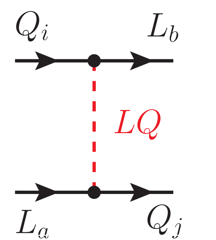
(a)

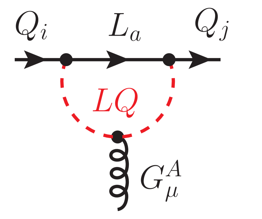
(b)

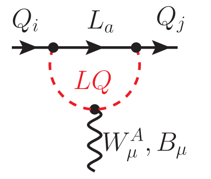
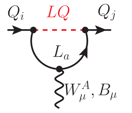
(c)

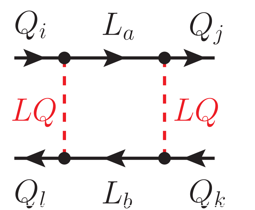
(d)

Figure 1: LQ Tree-level exchange (a) gives rise to semi-leptonic operators. One-loop contributions to $\varepsilon^{\prime}/\varepsilon$ from QCD-penguins (b), EW-penguins (c) and box-type diagrams (d). Here $Q=\{q_{L},u_{R},d_{R}\}$ and $L=\{\ell_{L},e_{R}\}$ are SM quark and lepton flavour eigenstates. The ${\mathrm{SU(3)_{c}}}\otimes{\mathrm{SU(2)_{L}}}\otimes{\mathrm{U(1)_{Y}}}$ gauge bosons are denoted as $G_{\mu}^{A}$, $W_{\mu}^{A}$ and $B_{\mu}$, respectively.

3.3 One-loop LQ decoupling

The NL-$\psi^{4}$ coefficients receive direct contributions at ${\mu_{\Lambda}}$ from the LQ decoupling first at one-loop. Loop-corrections constitute a principal problem in massive vector LQ models when no full UV completion is specified. In the lack of a UV completion, simple cut-off regularisation might be used [66], introducing an additional dependence on the cut-off scale. On the other hand this issue is of no concern in scalar LQ models, for which we will calculate these contributions in this section. There are QCD- and EW-penguin diagrams, Figure 1(b) and Figure 1(c), as well as box-type diagrams Figure 1(d).

3.3.1 QCD penguins

QCD-penguin diagrams with LQs can contribute to the three operators

$$\,[{\cal P}_{4}^{(q)}]_{ji} =[\bar{q}^{j}_{L}\gamma_{\mu}T^{A}q^{i}_{L}]\sum_{k}[\bar{Q}^{k}\gamma^{\mu}T^{A}Q^{k}],$$ (3.7)

$$[{\cal P}_{4}^{(d)}]_{ji} =[\bar{d}^{j}_{R}\gamma_{\mu}T^{A}d^{i}_{R}]\sum_{k}[\bar{Q}^{k}\gamma^{\mu}T^{A}Q^{k}], [{\cal P}_{4}^{(u)}]_{ji} =[\bar{u}^{j}_{R}\gamma_{\mu}T^{A}u^{i}_{R}]\sum_{k}[\bar{Q}^{k}\gamma^{\mu}T^{A}Q^{k}],$$

depending on the LQ model. These operators are meant to be normalised as in (3.1). The sum over flavour-diagonal quark currents

$$\sum_{k}[\bar{Q}^{k}\gamma^{\mu}T^{A}Q^{k}] \equiv\sum_{k}\left([\bar{q}^{k}_{L}\gamma^{\mu}T^{A}q^{k}_{L}]+[\bar{d}^{k}_{R}\gamma^{\mu}T^{A}d^{k}_{R}]+[\bar{u}^{k}_{R}\gamma^{\mu}T^{A}u^{k}_{R}]\right)$$ (3.8)

arises from the quark-flavour universal gluon coupling and the matching might be performed exploiting the generic formula given in [68] for the $b\to s\,gluon$ off-shell vertex, see appendix in [69] for more details. We refrain from a projection onto the operators in Table 1 because we will neglect the RG evolution from ${\mu_{\Lambda}}$ to ${\mu_{\rm ew}}$ for these operators , which is a loop correction due to self-mixing. This will simplify the matching of SMEFT on low-energy EFT at ${\mu_{\rm ew}}$. For FCNC down-type transitions one has

$$[{\cal C}_{4}^{(a)}]_{ji}({\mu_{\rm ew}}) =\frac{\alpha_{s}}{4\pi}r_{4,a}^{\rm LQ}\frac{\Sigma^{ji}_{\chi,{\rm LQ}}}{M_{\rm LQ}^{2}} (a =q,d)$$ (3.9)

with the constants

$$r_{4,a}^{S_{1}} =\frac{\delta_{aq}}{18}, r_{4,a}^{{\widetilde{S}}_{1}} =\frac{\delta_{ad}}{18}, r_{4,a}^{R_{2}} =\frac{\delta_{aq}}{18}, r_{4,a}^{{\widetilde{R}}_{2}} =\frac{\delta_{ad}}{9}, r_{4,a}^{S_{3}} =\frac{\delta_{aq}}{6},$$ (3.10)

where $\delta_{aq}$ and $\delta_{ad}$ are Kronecker symbols. The comparison with the EW mixing-induced contributions (3.5) shows the same dependence on $\Sigma^{ji}_{\rm LQ}$. Further they are enhanced by the ratio $\alpha_{s}/\alpha_{e}\ln^{-1}({\mu_{\Lambda}}/{\mu_{\rm ew}})$. Numerically this amounts to roughly $\approx 15\ln^{-1}({\mu_{\Lambda}}/{\mu_{\rm ew}})\in[3,7]$ for ${\mu_{\Lambda}}\in[1,10]$ TeV and ${\mu_{\rm ew}}=100$ GeV, aside from the constant factors $r_{4,a}^{\rm LQ}$ and corresponding ones in the SL-$\psi^{4}$ coefficients. However, as will be shown in detail below and given in (D.6), this numerical enhancement of QCD-penguin Wilson coefficients becomes outweighed by another numerical enhancement of EW-penguin Wilson coefficients below ${\mu_{\rm ew}}$ in the expression of $\varepsilon^{\prime}/\varepsilon$, leaving the EW mixing-induced contributions as the dominant contributions in most LQ models.

3.3.2 EW penguins

The one-loop contributions to $\varepsilon^{\prime}/\varepsilon$ from EW-penguin diagrams in Figure 1(c) at the scale ${\mu_{\Lambda}}$ are actually the next-to-leading order (NLO) corrections to contributions from the tree-level decoupling in Section 3.2, as will become evident once the RG evolution of SMEFT in Section 3.4 is taken into account. In fact, those diagrams in Figure 1(c) that at low energies represent QED penguin diagrams, contain infrared divergences that are cancelled in the matching on SMEFT by the ultraviolet divergences of diagrams with SL-$\psi^{4}$ insertions when closing the lepton lines to a loop and radiating off a ${\mathrm{SU(2)_{L}}}$ or ${\mathrm{U(1)_{Y}}}$ gauge boson respectively. These are the very same diagrams that determine the anomalous dimensions of SMEFT operators [65]. Parametrically such NLO EW-penguin terms contribute to the NL-$\psi^{4}$ Wilson coefficients as in (3.5), just without the logarithmic enhancement and therefore we will not further consider them throughout.

3.3.3 Box diagrams

The most general quark transitions $Q_{i}\bar{Q}_{k}\to Q_{j}\bar{Q}_{l}$ from LQ box diagrams with $Q=(q_{L},d_{R},u_{R})$ generate in SMEFT

$${\cal L}_{\rm SMEFT} \supset\sum_{a}\sum_{jikl}[{\cal C}_{a}^{(o)}]_{jikl}\,[{\cal P}_{a}^{(o)}]_{jikl}$$ (3.11)

with non-leptonic operators of colour-octet type

$$\,\![{\cal P}_{qq}^{(o,1)}]_{jikl} =[\bar{q}^{j,\alpha}_{L}\gamma_{\mu}q^{i,\beta}_{L}][\bar{q}^{k,\beta}_{L}\gamma^{\mu}q^{l,\alpha}_{L}], S_{1}(LL),R_{2}(RR),S_{3},U_{1}(LL),U_{3}$$ (3.12)

$$[{\cal P}_{qq}^{(o,3)}]_{jikl} =[\bar{q}^{j,\alpha}_{L}\gamma_{\mu}\tau^{I}q^{i,\beta}_{L}][\bar{q}^{k,\beta}_{L}\gamma^{\mu}\tau^{I}q^{l,\alpha}_{L}], R_{2}(RR),S_{3},V_{2}(RR),U_{3}$$

$$[{\cal P}_{dd}^{(o)}]_{jikl} =[\bar{d}^{j,\alpha}_{R}\gamma_{\mu}d^{i,\beta}_{R}][\bar{d}^{k,\beta}_{R}\gamma^{\mu}d^{l,\alpha}_{R}], {\widetilde{S}}_{1},{\widetilde{R}}_{2},U_{1}(RR),V_{2}(LL)$$

$$[{\cal P}_{qd}^{(o)}]_{jikl} =[\bar{q}^{j,\alpha}_{L}\gamma_{\mu}q^{i,\beta}_{L}][\bar{d}^{k,\beta}_{R}\gamma^{\mu}d^{l,\alpha}_{R}], U_{1}(LR),V_{2}(RL)$$

$$[{\cal P}_{qu}^{(o)}]_{jikl} =[\bar{q}^{j,\alpha}_{L}\gamma_{\mu}q^{i,\beta}_{L}][\bar{u}^{k,\beta}_{R}\gamma^{\mu}u^{l,\alpha}_{R}], S_{1}(LR),R_{2}(RL)$$

where $\alpha,\,\beta$ denote ${\mathrm{SU(3)_{c}}}$ colour indices. Here we have retained only those that contribute to down-type quark transitions and show corresponding LQ models that give rise to each operator. Included are the combinations of chirality $\chi\chi^{\prime}$ of the couplings $\Sigma_{\chi}^{ji}\Sigma_{\chi^{\prime}}^{kl}$ for LQ models with two couplings ($U_{1},V_{2},S_{1},R_{2})$ that can be easily understood from (A.1) and (A.2). They are linear combinations of the NL-$\psi^{4}$ operators in Table 1: ${\cal O}_{qq,qd,qu}^{(1,8)},\,{\cal O}_{dd}$, which can be seen upon using

$$T^{A}_{ij}T^{A}_{kl} =\frac{1}{2}\left(\delta_{il}\delta_{jk}-\frac{1}{N_{c}}\delta_{ij}\delta_{kl}\right),$$ (3.13)

or in the case of ${\cal P}_{qq,dd}^{(\ldots)}$ Fierz relations.

The explicit matching results of the Wilson coefficients $[{\cal C}_{a}^{(o,\dots)}]_{jikl}$ at ${\mu_{\Lambda}}$ for scalar LQ models $S_{1,3},{\widetilde{S}}_{1},R_{2}$ and ${\widetilde{R}}_{2}$ are provided in Appendix C. We will omit the RG evolution from ${\mu_{\Lambda}}$ to ${\mu_{\rm ew}}$ as in the case of QCD penguin contributions. A main distinguishing feature of boxes compared to QCD and EW penguins is that the gauge coupling is replaced by an additional combination of LQ couplings

$$[{\cal C}_{a}^{(o)}]_{jikl} \propto\frac{\Sigma^{kl}_{\chi^{\prime}}}{(4\pi)^{2}}\frac{\Sigma^{ji}_{\chi}}{M^{2}_{\rm LQ}}.$$ (3.14)

3.4 Renormalisation Group Equations

The RG equations have the general structure

$$\dot{\cal C}_{a} \equiv(4\pi)^{2}\mu\frac{{\rm d}{\cal C}_{a}}{{\rm d}\mu}=\gamma_{ab}\,{\cal C}_{b}$$ (3.15)

with $\gamma_{ab}$ being the entries of a very big anomalous dimension matrix (ADM). The ADM is known for SMEFT at one-loop and the entries relevant here have been presented in [65]. For small $\gamma_{ab}/(4\pi)^{2}\ll 1$ the approximate solution retains only the first leading logarithm (1stLLA)

$${\cal C}_{a}({\mu_{\rm ew}}) =\left[\delta_{ab}-\frac{\gamma_{ab}}{(4\pi)^{2}}\ln\frac{{\mu_{\Lambda}}}{{\mu_{\rm ew}}}\right]{\cal C}_{b}({\mu_{\Lambda}}),$$ (3.16)

which is sufficient as long as the logarithm is not too large, so that also $\gamma_{ab}/(4\pi)^{2}\ln\frac{{\mu_{\Lambda}}}{{\mu_{\rm ew}}}\ll 1$ holds. We should stress that RG effects due to top-quark Yukawa mixing considered recently in various analyses [59, 60, 24] are absent here [64].

In what follows we list RG equations which govern the generation of NL-$\psi^{4}$ coefficients from SL-$\psi^{4}$ ones. For NL-$\psi^{4}$ $(\bar{L}L)(\bar{L}L)$ operators we find using [65]

$$[\dot{\cal C}_{qq}^{(1)}]_{prst} =-\frac{1}{9}g^{2}_{1}\left([{\cal C}_{\ell q}^{(1)}]_{wwst}\delta_{pr}+[{\cal C}_{\ell q}^{(1)}]_{wwpr}\delta_{st}+[{\cal C}_{qe}]_{stww}\delta_{pr}+[{\cal C}_{qe}]_{prww}\delta_{st}\right),$$ (3.17)

$$[\dot{\cal C}_{qq}^{(3)}]_{prst} =+\frac{1}{3}g^{2}_{2}\left([{\cal C}_{\ell q}^{(3)}]_{wwst}\delta_{pr}+[{\cal C}_{\ell q}^{(3)}]_{wwpr}\delta_{st}\right).$$ (3.18)

For NL-$\psi^{4}$ $(\bar{R}R)(\bar{R}R)$ operators we find

$$[\dot{\cal C}_{uu}]_{prst} =-\frac{4}{9}g^{2}_{1}\Big{(}[{\cal C}_{eu}]_{wwst}\delta_{pr}+[{\cal C}_{eu}]_{wwpr}\delta_{st}+[{\cal C}_{\ell u}]_{wwst}\delta_{pr}+[{\cal C}_{\ell u}]_{wwpr}\delta_{st}\Big{)},$$ (3.19)

$$[\dot{\cal C}_{dd}]_{prst} =+\frac{2}{9}g^{2}_{1}\Big{(}[{\cal C}_{ed}]_{wwst}\delta_{pr}+[{\cal C}_{ed}]_{wwpr}\delta_{st}+[{\cal C}_{\ell d}]_{wwst}\delta_{pr}+[{\cal C}_{\ell d}]_{wwpr}\delta_{st}\Big{)},$$ (3.20)

$$[\dot{\cal C}_{ud}^{(1)}]_{prst} =+\frac{4}{9}g^{2}_{1}\Big{(}[{\cal C}_{\ell u}]_{wwpr}\delta_{st}+[{\cal C}_{eu}]_{wwpr}\delta_{st}-2[{\cal C}_{\ell d}]_{wwst}\delta_{pr}-2[{\cal C}_{ed}]_{wwst}\delta_{pr}\Big{)}.$$ (3.21)

For NL-$\psi^{4}$ $(\bar{L}L)(\bar{R}R)$ operators we find

$$[\dot{\cal C}_{qu}^{(1)}]_{prst} =-\frac{2}{9}g^{2}_{1}\left(4[{\cal C}_{\ell q}^{(1)}]_{wwpr}\delta_{st}+4[{\cal C}_{qe}]_{prww}\delta_{st}+[{\cal C}_{\ell u}]_{wwst}\delta_{pr}+[{\cal C}_{eu}]_{wwst}\delta_{pr}\right),$$ (3.22)

$$[\dot{\cal C}_{qd}^{(1)}]_{prst} =+\frac{2}{9}g^{2}_{1}\left(2[{\cal C}_{\ell q}^{(1)}]_{wwpr}\delta_{st}+2[{\cal C}_{qe}]_{prww}\delta_{st}-[{\cal C}_{\ell d}]_{wwst}\delta_{pr}-[{\cal C}_{ed}]_{wwst}\delta_{pr}\right),$$ (3.23)

and finally for all other NL-$\psi^{4}$ operators

$$[\dot{\cal C}_{ud}^{(8)}]_{prst} =0, [\dot{\cal C}_{qu}^{(8)}]_{prst} =0, [\dot{\cal C}_{quqd}^{(1)}]_{prst} =0,$$ (3.24)

$$[\dot{\cal C}_{qd}^{(8)}]_{prst} =0, [\dot{\cal C}_{quqd}^{(8)}]_{prst} =0.$$

We observe that the ${\mathrm{SU(2)_{L}}}\otimes{\mathrm{U(1)_{Y}}}$ gauge-mixing of SL-$\psi^{4}$ into NL-$\psi^{4}$ operators within SMEFT generates in 1stLLA only $(\bar{L}L)(\bar{L}L)$, $(\bar{L}L)(\bar{R}R)$ and $(\bar{R}R)(\bar{R}R)$ NL-$\psi^{4}$ operators from the corresponding semi-leptonic classes. The initial Wilson coefficients of the semi-leptonic operators at the scale ${\mu_{\Lambda}}$ enter only summed over the lepton-flavour diagonal parts $[{\cal C}_{b}^{(a)}]_{ww\cdot\cdot}$ (and $[{\cal C}_{qe}]_{\cdot\cdot ww}$), summation over the index $w=1,2,3$ is implied, because all leptons can run inside the loop. In consequence the underlying combination of LQ couplings is $\Sigma^{ji}_{\rm LQ}$, introduced in (3.6). Further, the NL-$\psi^{4}$ Wilson coefficients at ${\mu_{\rm ew}}$ contain always one quark-flavour diagonal quark-bilinear since all ADMs are $\propto\delta_{st}$ or $\delta_{pr}$ and as a consequence some terms will not contribute to down-type $\Delta F=1$ processes.

The $({\overline{L}}R)({\overline{R}}L)$ and $({\overline{L}}R)({\overline{L}}R)$ SL-$\psi^{4}$ operators ${\cal O}_{\ell edq}$ and ${\cal O}_{\ell equ}^{(1,3)}$ are only needed if they contribute to semi-leptonic $K$ decays in order to derive constraints on the LQ couplings. On the other hand, $({\overline{L}}R)({\overline{L}}R)$ NL-$\psi^{4}$ operators ${\cal O}_{quqd}^{(1,3)}$ contribute to $\varepsilon^{\prime}/\varepsilon$ only in those LQ models that provide a direct one-loop matching contribution at ${\mu_{\Lambda}}$, i.e. ${\cal P}^{(o)}_{qd,\,qu}$ in (3.12).

The RG equations provide the Wilson coefficients of the SMEFT operators at the electroweak scale ${\mu_{\rm ew}}$, where electroweak symmetry breaking (EWSB) takes place. At this point the transition from the weak to the mass eigenbasis for gauge, quark and lepton fields can be done within SMEFT. The quark fields are rotated by $3\times 3$ unitary rotations in flavour space

$$\psi_{L} \to V^{\psi}_{L}\psi_{L}\,, \psi_{R} \to V^{\psi}_{R}\psi_{R}\,,$$ (3.25)

for $\psi=u,d$, such that

$$V^{\psi\dagger}_{L}m_{\psi}V^{\psi}_{R} =m_{\psi}^{\rm diag}, V \equiv(V^{u}_{L})^{\dagger}V^{d}_{L}\,,$$ (3.26)

with diagonal up- and down-quark mass matrices $m_{\psi}^{\rm diag}$. In general, the non-diagonal mass matrices $m_{\psi}$ include the contributions of dim-6 operators. The quark-mixing matrix $V$ is unitary, similar to the CKM matrix of the SM; however, in the presence of dim-6 contributions the numerical values are different from those obtained in usual SM CKM-fits. Since we are interested in down-type processes $\varepsilon^{\prime}/\varepsilon$ and rare Kaon processes, we will take the freedom to choose the weak basis such that down-type quarks are already mass eigenstates, which fixes $V_{L,R}^{d}=\leavevmode\hbox{\small 1\kern-3.6pt\normalsize 1}$, and assume without loss of generality $V_{R}^{u}=\leavevmode\hbox{\small 1\kern-3.6pt\normalsize 1}$, yielding $q_{L}=(V^{\dagger}u_{L},d_{L})^{T}$. Analogously, we choose also the down-type lepton mass matrix to be diagonal and leave the neutrinos in the flavour eigenbasis. This defines the SMEFT Wilson coefficients unambiguously and avoids the appearance of the PMNS lepton-mixing matrix in interactions involving neutrinos.

3.5 Non-leptonic operators: SMEFT on $\Delta F=1$ EFT

The tree-level matching of SMEFT on $\Delta F=1$ low-energy EFT’s at the scale ${\mu_{\rm ew}}$ is well-known for semi-leptonic processes [70, 28, 71] and given for non-leptonic processes in [72]. We summarise the required parts in the following three subsections. Starting with non-leptonic operators, we provide results relevant for $\varepsilon^{\prime}/\varepsilon$ for the choice of the traditional basis of the QCD- and EW-penguin operators (2.1) and (2.2), which differs from [67], and simplifies due to the particular flavour structure (3.17) – (3.23) of the EW gauge-mixing of SL-$\psi^{4}$ into NL-$\psi^{4}$ SMEFT operators. Further we summarise the tree-level matching of SL-$\psi^{4}$ operators relevant for $d_{i}\ell_{a}\to d_{j}\ell_{b}$, $d_{i}\nu_{a}\to d_{j}\nu_{b}$ and $d_{i}\nu_{a}\to u_{j}\ell_{b}$.

3.5.1 EW gauge-mixing

As already pointed out in Section 3.4, the EW gauge-mixing of SL-$\psi^{4}$ into NL-$\psi^{4}$ operators leads to flavour-universal down-type and up-type contributions that correspond almost exclusively to linear combinations of QCD- and EW-penguin operators ($e_{u}=-2e_{d}=+2/3$)

$$(\bar{s}d)_{V-A}\,\sum_{u}(\bar{u}u)_{V-A} =\frac{1}{3}(Q_{3}+2Q_{9}), (\bar{s}d)_{V-A}\,\sum_{d}(\bar{d}d)_{V-A} =\frac{2}{3}(Q_{3}-Q_{9}),$$ (3.27)

$$(\bar{s}d)_{V-A}\,\sum_{u}(\bar{u}u)_{V+A} =\frac{1}{3}(Q_{5}+2Q_{7}), (\bar{s}d)_{V-A}\,\sum_{d}(\bar{d}d)_{V+A} =\frac{2}{3}(Q_{5}-Q_{7}),$$

and analogously for chirality-flipped $Q^{\prime}_{3,5,7,9}$ — see definitions (2.1) and (2.2), except for one contribution from ${\cal O}_{qq}^{(3)}$ as shown below.

Let us illustrate in some detail the matching for the $(\bar{L}L)(\bar{R}R)$ NL-$\psi^{4}$ operators ${\cal O}_{qd}^{(1)}$ and ${\cal O}_{qu}^{(1)}$. The ADM given in (3.23) yields upon insertion into (3.16) at the scale ${\mu_{\rm ew}}$

$$[{\cal C}_{qd}^{(1)}]_{prst}[{\cal O}_{qd}^{(1)}]_{prst}=-\frac{2}{9}\frac{g_{1}^{2}}{(4\pi)^{2}}\ln\frac{{\mu_{\Lambda}}}{{\mu_{\rm ew}}}\;\left(2\big{[}{\cal C}_{\ell q}^{(1)}+{\cal C}_{qe}\big{]}_{wwpr}\delta_{st}-\big{[}{\cal C}_{\ell d}+{\cal C}_{de}\big{]}_{wwst}\delta_{pr}\right)$$

$$\hskip 85.35826pt\times\left[(\bar{u}_{L}^{p}\gamma_{\mu}u_{L}^{r})+(\bar{d}_{L}^{p}\gamma_{\mu}d_{L}^{r})\right](\bar{d}_{R}^{s}\gamma^{\mu}d_{R}^{t}).$$ (3.28)

The $$\delta_{pr,st} \bar{d}^{p}_{R(L)}\to\bar{s}P_{L(R)} d^{r}_{R(L)}\to P_{R(L)}d \bar{s}\to\bar{d} P_{R,L}=(1\pm\gamma_{5})/2$$-symbols give rise to the aforementioned flavour-diagonal quark-bilinears. In the transition to mass eigenstates after EWSB, we keep only terms with and that contribute to transitions ()

$$\simeq-\frac{1}{9}\frac{\alpha_{e}}{4\pi}\ln\frac{{\mu_{\Lambda}}}{{\mu_{\rm ew}}}\;\frac{\big{[}{\cal C}_{\ell q}^{(1)}+{\cal C}_{qe}\big{]}_{ww21}}{c_{W}^{2}}\;(\bar{s}d)_{V-A}\sum_{d}(\bar{d}d)_{V+A}$$ (3.29)

$$\phantom{\to}+\frac{1}{18}\frac{\alpha_{e}}{4\pi}\ln\frac{{\mu_{\Lambda}}}{{\mu_{\rm ew}}}\;\frac{\big{[}{\cal C}_{\ell d}+{\cal C}_{de}\big{]}_{ww21}}{c_{W}^{2}}\;(\bar{s}d)_{V+A}\left[\sum_{d}(\bar{d}d)_{V-A}+\sum_{k,i,j}V_{ik}V_{jk}^{\ast}(\bar{u}^{i}u^{j})_{V-A}\right].$$

Finally one finds with the unitarity of the mixing matrix $$\sum_{k}V_{ik}V_{jk}^{*}=\delta_{ij}$$ and relations (3.27)

$$\simeq\frac{\alpha_{e}}{4\pi}\ln\frac{{\mu_{\Lambda}}}{{\mu_{\rm ew}}}\left(-\frac{2}{27}\frac{\big{[}{\cal C}_{\ell q}^{(1)}+{\cal C}_{qe}\big{]}_{ww21}}{c_{W}^{2}}(Q_{5}-Q_{7})+\frac{1}{18}\frac{\big{[}{\cal C}_{\ell d}+{\cal C}_{de}\big{]}_{ww21}}{c_{W}^{2}}\,Q^{\prime}_{5}\right)$$ (3.30)

and similarly for the operator

$$[{\cal C}_{qu}^{(1)}]_{prst}[{\cal O}_{qu}^{(1)}]_{prst}\simeq\frac{\alpha_{e}}{4\pi}\ln\frac{{\mu_{\Lambda}}}{{\mu_{\rm ew}}}\frac{2}{27}\frac{\big{[}{\cal C}_{\ell q}^{(1)}+{\cal C}_{qe}\big{]}_{ww21}}{c_{W}^{2}}(Q_{5}+2Q_{7}).$$ (3.31)

The total contribution of $(\bar{L}L)(\bar{R}R)$ operators is

$$[{\cal C}_{qu}^{(1)}]_{prst} [{\cal O}_{qu}^{(1)}]_{prst}+[{\cal C}_{qd}^{(1)}]_{prst}[{\cal O}_{qd}^{(1)}]_{prst}$$ (3.32)

$$\simeq\frac{\alpha_{e}}{4\pi}\frac{\big{[}{\cal C}_{\ell q}^{(1)}+{\cal C}_{qe}\big{]}_{ww21}}{c_{W}^{2}}\frac{2}{9}\ln\frac{{\mu_{\Lambda}}}{{\mu_{\rm ew}}}Q_{7}+\frac{\alpha_{e}}{4\pi}\frac{\big{[}{\cal C}_{\ell d}+{\cal C}_{de}\big{]}_{ww21}}{c_{W}^{2}}\frac{1}{18}\ln\frac{{\mu_{\Lambda}}}{{\mu_{\rm ew}}}Q^{\prime}_{5}$$

free of $Q_{5}$ and all SL-$\psi^{4}$ Wilson coefficients are at the scale ${\mu_{\Lambda}}$.

The results for the other cases $(\bar{R}R)(\bar{R}R)$ and $(\bar{L}L)(\bar{L}L)$ are obtained analogously,

$$[{\cal C}_{dd}]_{prst}[{\cal O}_{dd}]_{prst}+[{\cal C}_{ud}^{(1)}]_{prst}[{\cal O}_{ud}^{(1)}]_{prst} \simeq\frac{\alpha_{e}}{4\pi}\;\frac{\big{[}{\cal C}_{\ell d}+{\cal C}_{ed}\big{]}_{ww21}}{c_{W}^{2}}\;\frac{2}{9}\ln\frac{{\mu_{\Lambda}}}{{\mu_{\rm ew}}}Q^{\prime}_{9},$$ (3.33)

$$[{\cal C}_{qq}^{(1)}]_{prst}[{\cal O}_{qq}^{(1)}]_{prst} \simeq\frac{\alpha_{e}}{4\pi}\;\frac{\big{[}{\cal C}_{\ell q}^{(1)}+{\cal C}_{qe}\big{]}_{ww21}}{c_{W}^{2}}\;\frac{1}{18}\ln\frac{{\mu_{\Lambda}}}{{\mu_{\rm ew}}}Q_{3},$$ (3.34)

where an additional term arises for ${\cal O}_{qq}^{(3)}$

$$[{\cal C}_{qq}^{(3)}]_{prst} [{\cal O}_{qq}^{(3)}]_{prst}\simeq\frac{\alpha_{e}}{4\pi}\;\frac{[{\cal C}_{\ell q}^{(3)}]_{ww21}}{s_{W}^{2}}\;\frac{1}{18}\ln\frac{{\mu_{\Lambda}}}{{\mu_{\rm ew}}}\left(4\,Q_{9}-Q_{3}\right)$$ (3.35)

$$\hskip 5.69046pt-\frac{\alpha_{e}}{4\pi}\;\sum_{k,ij}\left(V_{i1}V_{jk}^{\ast}\frac{[{\cal C}_{\ell q}^{(3)}]_{ww2k}}{s_{W}^{2}}+V_{ik}V_{j2}^{\ast}\frac{[{\cal C}_{\ell q}^{(3)}]_{wwk1}}{s_{W}^{2}}\right)\frac{1}{3}\ln\frac{{\mu_{\Lambda}}}{{\mu_{\rm ew}}}(\bar{s}d)_{V-A}(\bar{u}^{i}u^{j})_{V-A}.$$

Although new physics can affect the quark-mixing matrix $V$ to deviate from the SM CKM matrix, we assume that these effects do not lift the hierarchy in the Cabibbo-angle $\lambda_{C}$ represented by the Wolfenstein parameterisation and found in SM CKM fits. Assuming further that the Wilson coefficients $[{\cal C}_{\ell q}^{(3)}]_{wwk^{\prime}k}$ do not lift this hierarchy either, the additional term in ${\cal O}_{qq}^{(3)}$ becomes

$$\sum_{k,ij} \left(V_{i1}V_{jk}^{\ast}\frac{[{\cal C}_{\ell q}^{(3)}]_{ww2k}}{s_{W}^{2}}+V_{ik}V_{j2}^{\ast}\frac{[{\cal C}_{\ell q}^{(3)}]_{wwk1}}{s_{W}^{2}}\right)(\bar{s}d)_{V-A}(\bar{u}^{i}u^{j})_{V-A}$$ (3.36)

$$=\frac{[{\cal C}_{\ell q}^{(3)}]_{ww21}}{s_{W}^{2}}(\bar{s}d)_{V-A}\Big{[}|V_{11}|^{2}(\bar{u}u)_{V-A}+|V_{22}|^{2}(\bar{c}c)_{V-A}\Big{]}$$

$$+(\bar{s}d)_{V-A}(\bar{u}c)_{V-A}\frac{V_{11}V_{22}^{\ast}}{s_{W}^{2}}\Big{(}[{\cal C}_{\ell q}^{(3)}]_{ww22}+[{\cal C}_{\ell q}^{(3)}]_{ww11}\Big{)}+{\cal O}(\lambda_{C}).$$

The $(\bar{u}c)_{V-A}$ part in the last line does not contribute to $\varepsilon^{\prime}/\varepsilon$, whereas the $i=j=c$ part is loop-suppressed in principle. We still keep the latter and use $|V_{11}|^{2}=|V_{22}|^{2}\approx 1+{\cal O}(\lambda_{C})$ as well as (3.27) to arrive at

$$\mbox{eq.}~{}(\ref{eq:qq-3-intermediate}) =\frac{[{\cal C}_{\ell q}^{(3)}]_{ww21}}{s_{W}^{2}}\frac{1}{3}(Q_{3}+2Q_{9}).$$ (3.37)

The matching conditions of $\Delta S=1$ operators (D.1) at ${\mu_{\rm ew}}$ are given in terms of the SL-$\psi^{4}$ Wilson coefficients at ${\mu_{\Lambda}}$

$$C_{3}({\mu_{\rm ew}}) =-\frac{1}{9}\frac{\alpha_{e}}{4\pi}\frac{v^{2}}{c_{W}^{2}}\frac{\big{[}{\cal C}_{\ell q}^{(1)}+{\cal C}_{qe}\big{]}_{ww21}}{\lambda_{u}^{sd}}\ln\frac{{\mu_{\Lambda}}}{{\mu_{\rm ew}}}+\frac{1}{3}\frac{\alpha_{e}}{4\pi}\frac{v^{2}}{s_{W}^{2}}\frac{[{\cal C}_{\ell q}^{(3)}]_{ww21}}{\lambda_{u}^{sd}}\ln\frac{{\mu_{\Lambda}}}{{\mu_{\rm ew}}},$$ (3.38)

$$C_{7}({\mu_{\rm ew}}) =-\frac{4}{9}\frac{\alpha_{e}}{4\pi}\frac{v^{2}}{c_{W}^{2}}\frac{\big{[}{\cal C}_{\ell q}^{(1)}+{\cal C}_{qe}\big{]}_{ww21}}{\lambda_{u}^{sd}}\ln\frac{{\mu_{\Lambda}}}{{\mu_{\rm ew}}},$$

$$C^{\prime}_{9}({\mu_{\rm ew}}) =4\,C^{\prime}_{5}({\mu_{\rm ew}})=-\frac{4}{9}\frac{\alpha_{e}}{4\pi}\frac{v^{2}}{c_{W}^{2}}\frac{\big{[}{\cal C}_{\ell d}+{\cal C}_{ed}\big{]}_{ww21}}{\lambda_{u}^{sd}}\ln\frac{{\mu_{\Lambda}}}{{\mu_{\rm ew}}},$$

where $v^{2}=(\sqrt{2}G_{F})^{-1}$ and $c_{W}\equiv\cos\theta_{W}$. We used the approximation (3.37). These three expressions are fundamental for EW-mixing effects in $\varepsilon^{\prime}/\varepsilon$ in LQ models.

There are three possible patterns of contributions to $\varepsilon^{\prime}/\varepsilon$ listed in Table 2, showing also that LQ models ${\widetilde{U}}_{1}$ and ${\widetilde{V}}_{2}$ do not contribute to $\varepsilon^{\prime}/\varepsilon$ via EW gauge-mixing. In most models $\varepsilon^{\prime}/\varepsilon$ is affected by $\Sigma^{ji}_{\chi,{\rm LQ}}$ with either $\chi=L$ or $\chi=R$, but not both, the exceptions are vector LQ models $U_{1}$ and $V_{2}$. For the first pattern involving $C_{3,7}$, the numerically largest impact on $\varepsilon^{\prime}/\varepsilon$ will be due to the contribution from $C_{7}({\mu_{\rm ew}})$ — see (D.6) and Table 5 — either due to ${\cal C}_{\ell q}^{(1)}$ or ${\cal C}_{qe}$, such that ${\cal C}_{\ell q}^{(3)}$ is numerically irrelevant for $\varepsilon^{\prime}/\varepsilon$. Let us note that in LQ models ${\cal C}_{\ell q}^{(3)}$ and ${\cal C}_{\ell q}^{(1)}$ are not independent from each other but related through ${\cal C}_{\ell q}^{(3)}\equiv r_{\rm LQ}\,{\cal C}_{\ell q}^{(1)}$ with

$$r_{S_{1}} =-1, r_{S_{3}} =\frac{1}{3}, r_{U_{1}} =1, r_{U_{3}} =-\frac{1}{3},$$ (3.39)

see Appendix B. In the second pattern with $C^{\prime}_{5,9}$ the largest impact will be due to $C^{\prime}_{9}=4\,C^{\prime}_{5}$, where the $C^{\prime}_{5}$ contributes constructively. The third case of $C_{3,7}$ and $C^{\prime}_{5,9}$ involves both $\chi=L$ and $\chi=R$ LQ couplings, which can be in principle of different size and prevent an apriori estimate of the relative numerical sizes of all contributions, although $C_{7}$ is roughly enhanced by a factor of sixty compared to $C^{\prime}_{9}$, see (D.6) and Table 5. The latter fact implies that models, which generate ${\cal C}_{\ell q}^{(1)}$ or ${\cal C}_{qe}$ can face easier the $\varepsilon^{\prime}/\varepsilon$ anomaly via the operator $Q_{7}$ than the other models.

LQ model	semi-leptonic SMEFT coeff.	$\Delta S=1$ coeff.
$S_{1,3}$, $U_{3}$	${\cal C}_{\ell q}^{(1,3)}$ ($L$)	$C_{3}$, $C_{7}$
$R_{2}$	${\cal C}_{qe}$ ($R$)
${\widetilde{S}}_{1}$	${\cal C}_{ed}$ ($R$)	$C^{\prime}_{5}$, $C^{\prime}_{9}$
${\widetilde{R}}_{2}$	${\cal C}_{\ell d}$ ($L$)
$U_{1}$	${\cal C}_{\ell q}^{(1,3)}$ ($L$), ${\cal C}_{ed}$ ($R$)	$C_{3}$, $C_{7}$, $C^{\prime}_{5}$, $C^{\prime}_{9}$
$V_{2}$	${\cal C}_{qe}$ ($R$), ${\cal C}_{\ell d}$ ($L$)

Table 2: Classification of LQ models corresponding to their contribution to $\varepsilon^{\prime}/\varepsilon$ via EW gauge-mixing and the involved semi-leptonic Wilson coefficient. The chirality of the LQ couplings entering the semi-leptonic Wilson coefficients is shown in parenthesis, see Appendix B for details.

3.5.2 QCD-penguins

Besides the EW mixing-induced contributions, the NL-$\psi^{4}$ coefficients receive direct one-loop matching contributions at ${\mu_{\Lambda}}$ from QCD- and EW-penguin diagrams as well as box-type diagrams. As already discussed in Section 3.3.1, QCD-penguin contributions are parametrically enhanced w.r.t. the mixing-induced contributions at ${\mu_{\rm ew}}$. After EWSB, the operators (3.7) are matched onto the $\Delta F=1$ low-energy analogue yielding

$$-3\,C_{3}=C_{4}=-3\,C_{5}=C_{6} =-\frac{v^{2}}{4}\frac{[{\cal C}_{4}^{(q)}]_{21}}{\lambda_{u}^{sd}}=-\frac{\alpha_{s}}{4\pi}\frac{v^{2}}{M_{\rm LQ}^{2}}\frac{r_{4,q}^{\rm LQ}}{4}\frac{\Sigma^{21}_{\rm LQ}}{\lambda_{u}^{sd}},$$ (3.40)

$$-3\,C_{3^{\prime}}=C_{4^{\prime}}=-3\,C_{5^{\prime}}=C_{6^{\prime}} =-\frac{v^{2}}{4}\frac{[{\cal C}_{4}^{(d)}]_{21}}{\lambda_{u}^{sd}}=-\frac{\alpha_{s}}{4\pi}\frac{v^{2}}{M_{\rm LQ}^{2}}\frac{r_{4,d}^{\rm LQ}}{4}\frac{\Sigma^{21}_{\rm LQ}}{\lambda_{u}^{sd}},$$

at ${\mu_{\rm ew}}$ using (3.9). This can be compared to the contributions from EW gauge-mixing (3.38), showing again the enhancement factor $\alpha_{s}/\alpha_{e}\ln^{-1}({\mu_{\Lambda}}/{\mu_{\rm ew}})$. Yet, as we will find in the next section at the end QCD penguin effects will be much smaller than EW gauge-mixing and box-diagram contributions that we discuss next.

3.5.3 Box diagrams

The LQ box-diagrams generate NL-$\psi^{4}$ operators (3.12) of which the majority do not contribute directly to $K\to\pi\pi$ transitions because the flavour indices do not involve the required ones. Yet some of these operators can contribute indirectly due to RG mixing into operators that contribute directly. We will first illustrate the matching for the various operators ${\cal P}_{dd}^{(o)}$, since here the transition from weak to mass eigenstates is trivial in the absence of $q_{L}$. Note that due to equal Lorentz structure in both quark currents there is a symmetry under simultaneous $i\leftrightarrow l$ and $j\leftrightarrow k$, such that we might fix $j=2$ since we are interested in $K\to\pi\pi$. For the time being we still use notational distinction $d^{i}_{R}\to P_{R}D_{i}$ between weak and mass eigenstates by using capital $D_{i}=(d,s,b)_{i}$ for latter ones

$${\cal L}_{\rm SMEFT} \supset\sum_{ikl}[{\cal C}_{dd}^{(o)}]_{2ikl}[\bar{d}^{2,\alpha}_{R}\gamma_{\mu}d^{i,\beta}_{R}][\bar{d}^{k,\beta}_{R}\gamma^{\mu}d^{l,\alpha}_{R}]$$

$$=\sum_{ikl}\frac{[{\cal C}_{dd}^{(o)}]_{2ikl}}{4}(\bar{s}^{\alpha}D_{i}^{\beta})_{V+A}(\bar{D}_{k}^{\beta}D_{l}^{\alpha})_{V+A}.$$ (3.41)

The operators with non-vanishing matrix elements to $$K\to\pi\pi d ikl=111 \Delta S=1 K\to\pi\pi d i=1 l=1 2 3 ikl=111$$ are those that contain three -quarks: . For other operators to contribute to the transition , at least one quark is required: or , as well as the remaining two indices should be equal (either or , as is already covered above), because only then they contribute via mixing into QCD- and EW-penguin operators when closing the quark loop and radiating off either gluon or photon in the low-energy EFT (same effects in SMEFT were neglected above). Thus the sum can be split into

$$=\frac{[{\cal C}_{dd}^{(o)}]_{2111}}{4}\;(\bar{s}^{\alpha}d^{\beta})_{V+A}(\bar{d}^{\beta}d^{\alpha})_{V+A}$$

$$+\frac{1}{4}\sum_{k\neq 1}\left([{\cal C}_{dd}^{(o)}]_{21kk}(\bar{s}^{\alpha}d^{\beta})_{V+A}(\bar{D}_{k}^{\beta}D_{k}^{\alpha})_{V+A}+[{\cal C}_{dd}^{(o)}]_{2kk1}(\bar{s}^{\alpha}D_{k}^{\beta})_{V+A}(\bar{D}_{k}^{\beta}d^{\alpha})_{V+A}\right)$$

$$+\frac{1}{4}\sum_{ikl}[{\cal C}_{dd}^{(o)}]_{2ikl}(\bar{s}^{\alpha}D_{i}^{\beta})_{V+A}(\bar{D}_{k}^{\beta}D_{l}^{\alpha})_{V+A}$$ (3.42)

where the terms in the last line are such that they do not contribute to $$K\to\pi\pi k=3 k$$ and are not part of the 1st and 2nd line. The 2nd term in the 2nd line contains actually only , due to the aforementioned symmetry. We rewrite the first term into a sum over , yielding shifts of the Wilson coefficients in the 2nd line

$$=\frac{[{\cal C}_{dd}^{(o)}]_{2111}}{4}\;(\bar{s}^{\alpha}d^{\beta})_{V+A}\sum_{k}(\bar{D}_{k}^{\beta}D_{k}^{\alpha})_{V+A}$$

$$+\frac{1}{4}\sum_{k\neq 1}\left([{\cal C}_{dd}^{(o)}]_{21kk}-[{\cal C}_{dd}^{(o)}]_{2111}\right)(\bar{s}^{\alpha}d^{\beta})_{V+A}(\bar{D}_{k}^{\beta}D_{k}^{\alpha})_{V+A}+\ldots$$ (3.43)

where the dots indicate the remaining terms in (3.42) and make use of (3.27), taking into account the different colour structure,

$$=\frac{[{\cal C}_{dd}^{(o)}]_{2111}}{4}\;\frac{2}{3}\left(Q_{4^{\prime}}-Q_{10^{\prime}}\right)$$

$$+\frac{1}{4}\sum_{k\neq 1}\left([{\cal C}_{dd}^{(o)}]_{21kk}-[{\cal C}_{dd}^{(o)}]_{2111}\right)(\bar{s}^{\alpha}d^{\beta})_{V+A}(\bar{D}_{k}^{\beta}D_{k}^{\alpha})_{V+A}+\ldots$$ (3.44)

In this way we have rewritten the operator $(\bar{s}d)(\bar{d}d)$ into QCD- and EW-penguin operators and the operators $(\bar{s}d)(\bar{s}s)$ and $(\bar{s}d)(\bar{b}b)$, which is a convenient choice of basis for $K\to\pi\pi$. Taking into account normalisation factors (D.1), it follows at ${\mu_{\rm ew}}$

$$C_{4^{\prime}}=-C_{10^{\prime}} =-\frac{v^{2}}{3}\frac{[{\cal C}_{dd}^{(o)}]_{2111}}{\lambda_{u}^{sd}}.$$ (3.45)

Although operators $\sim(\bar{s}d)(\bar{s}s)$ and $\sim(\bar{s}d)(\bar{b}b)$ are loop suppressed in $\varepsilon^{\prime}/\varepsilon$ w.r.t. $(\bar{s}d)(\bar{d}d)$ since they enter via RG mixing only, their Wilson coefficients might be numerically enhanced to overcome the loop-suppression because they depend on different combinations of LQ couplings. The mixing of $(\bar{s}d)(\bar{s}s)$ and $(\bar{s}d)(\bar{b}b)$ into QCD- and EW-penguins can be found in the literature as for example [58], but we will neglect these effects here.

The operators ${\cal P}^{(o,1)}_{qq}$ and ${\cal P}^{(o,3)}_{qq}$ contribute to $K\to\pi\pi$ as

$$C_{4} =-\frac{v^{2}}{6}\frac{\sum_{ji}(V_{1j}V_{1i}^{\ast}+2\delta_{1j}\delta_{1i})[{\cal C}_{qq}^{(o,1)}]_{21ji}}{\lambda_{u}^{sd}},$$ (3.46)

$$C_{10} =-\frac{v^{2}}{3}\frac{\sum_{ji}(V_{1j}V_{1i}^{\ast}-\delta_{1j}\delta_{1i})[{\cal C}_{qq}^{(o,1)}]_{21ji}}{\lambda_{u}^{sd}},$$

and

$$C_{9}=2\,C_{3} =-\frac{2v^{2}}{3}\frac{\sum_{ji}V_{1j}V_{1i}^{\ast}\;[{\cal C}_{qq}^{(o,3)}]_{2ji1}}{\lambda_{u}^{sd}},$$ (3.47)

$$C_{4} =-\frac{v^{2}}{6}\frac{\sum_{ji}(-V_{1j}V_{1i}^{\ast}+2\delta_{1j}\delta_{1i})[{\cal C}_{qq}^{(o,3)}]_{21ji}}{\lambda_{u}^{sd}},$$

$$C_{10} =-\frac{v^{2}}{3}\frac{\sum_{ji}(-V_{1j}V_{1i}^{\ast}-\delta_{1j}\delta_{1i})[{\cal C}_{qq}^{(o,3)}]_{21ji}}{\lambda_{u}^{sd}}.$$

The presence of $u_{L}$ in these operators leads to additional factors of the quark-mixing matrix $V$ with summation over $\Sigma^{ji}_{\chi}$.

The contribution to $K\to\pi\pi$ from ${\cal P}^{(o)}_{qu}$ is found analogously to be

$$C_{8}=2\,C_{6} =-\frac{v^{2}}{3}\frac{[{\cal C}_{qu}^{(o)}]_{2111}}{\lambda_{u}^{sd}}.$$ (3.48)

By comparison with (3.12), this shows that in models $S_{1}$ and $R_{2}$ the boxes give rise to the EW-penguin operators $Q_{6}$ and $Q_{8}$, where $Q_{8}$ is strongly enhanced in $\varepsilon^{\prime}/\varepsilon$. The matching contributions given in Appendix C with $[{\cal C}_{qu}^{(o)}]_{2111}\propto\Sigma^{11}_{R}\Sigma^{21}_{L}$ and $[{\cal C}_{qu}^{(o)}]_{2111}\propto\Sigma^{11}_{L}\Sigma^{12}_{R}$ for $S_{1}$ and $R_{2}$ respectively, show that these contributions depend on both chirality couplings $\chi=L,R$. This goes hand in hand with the $\Delta F=2$ operator for $D{\overline{D}}$-mixing analogous to $Q_{{\rm LR},2}^{ji}$ in (2.36) that is strongly enhanced by QCD RG evolution, and which depends on the combinations $\Sigma^{21}_{R}\Sigma^{21}_{L}$ and $\Sigma^{12}_{L}\Sigma^{12}_{R}$, respectively.

With similar considerations, the contribution to $K\to\pi\pi$ from ${\cal P}^{(o)}_{qd}$ is found to be

$$C_{6}=-C_{8} =-\frac{v^{2}}{3}\frac{[{\cal C}_{qd}^{(o)}]_{2111}}{\lambda_{u}^{sd}}, \qquad C_{6^{\prime}} =-\frac{v^{2}}{6}\frac{\sum_{ji}(V_{1j}V_{1i}^{\ast}+2\delta_{1j}\delta_{1i})[{\cal C}_{qd}^{(o)}]_{ji21}}{\lambda_{u}^{sd}},$$ (3.49)

$$C_{8^{\prime}} =-\frac{v^{2}}{3}\frac{\sum_{ji}(V_{1j}V_{1i}^{\ast}-\delta_{1j}\delta_{1i})[{\cal C}_{qd}^{(o)}]_{ji21}}{\lambda_{u}^{sd}}.$$

Note that $C_{8^{\prime}}$ is Cabibbo-suppressed w.r.t. $C_{6^{\prime}}$ and $C_{6,8}$, if one were to use $|V_{ud}|^{2}\approx 1$. Again operators $Q_{8,8^{\prime}}$ are strongly enhanced in $\varepsilon^{\prime}/\varepsilon$ such that for the corresponding models $U_{1}$ and $V_{2}$, see (3.12), these box-contributions could become important depending on the size of the $\Sigma^{ji}_{\chi}$. Although for vector LQs we are not able to calculate the coefficients ${\cal C}_{qd}^{(o)}$ without introducing cut-offs, still we can give their dependence on the $\Sigma^{ji}_{\chi}$.

In summary the three main contributions from LQ decoupling are due to 1) EW gauge-mixing of SL-$\psi^{4}$ into NL-$\psi^{4}$ operators, 2) QCD-penguins and 3) box diagrams. As a result the corresponding Wilson coefficients of QCD- and EW-penguin operators $C_{i}({\mu_{\rm ew}})$ ($i=3,\ldots,10$) scale parametrically as

$$\frac{e^{2}}{(4\pi)^{2}}\ln\frac{{\mu_{\Lambda}}}{{\mu_{\rm ew}}}\Sigma^{ji}_{\chi}\qquad\leftrightarrow\qquad\frac{g_{s}^{2}}{(4\pi)^{2}}\Sigma^{ji}_{\chi}\qquad\leftrightarrow\qquad\frac{\Sigma^{11}_{\chi^{\prime}}}{(4\pi)^{2}}\Sigma^{ji}_{\chi}.$$ (3.50)

Their relative sizes are thus fixed by $e^{2}\ln{\mu_{\Lambda}}/{\mu_{\rm ew}}\approx 0.1\ln{\mu_{\Lambda}}/{\mu_{\rm ew}}\approx 0.2\ldots 0.5$ for ${\mu_{\Lambda}}\in[1,\,20]$ TeV, and $g_{s}^{2}\approx 1.5$, whereas the yet-allowed size of the complex-valued $\Sigma^{11}_{\chi^{\prime}}$ is constrained by mostly tree-level processes, depending strongly on the LQ model. At the level of observables different suppression/enhancement factors for each of the $C_{i}({\mu_{\rm ew}})$ can appear such that at this point no definite conclusions can be drawn about which contribution is most important. We point out that concerning $\varepsilon^{\prime}/\varepsilon$, large enhancement of the EW-penguin coefficients $C_{7,8}({\mu_{\rm ew}})$ appear as can be seen from (D.6), which easily overcome the numerical enhancement of LQ-QCD-penguins discussed here and leads to the dominance of contributions due to EW gauge-mixing and/or LQ-boxes, depending on the LQ model.

3.6 Semi-leptonic operators: SMEFT on $\Delta F=1$ EFT

The $\Delta F=1$ semi-leptonic FCNC processes $d_{i}\ell_{a}\to d_{j}\ell_{b}$ and $d_{i}\nu_{a}\to d_{j}\nu_{b}$ are affected at tree-level by LQ exchange and provide strong constraints on LQ couplings. For practical purposes we neglect the running from ${\mu_{\Lambda}}$ to ${\mu_{\rm ew}}$ in SMEFT for the semi-leptonic operators if self-mixing is present in (3.16). The only exceptions are the models $S_{1}$ and $U_{1}$ because they predict at the scale ${\mu_{\Lambda}}$ the relation ${\cal C}_{\ell q}^{(1)}=\mp{\cal C}_{\ell q}^{(3)}$, see (3.39). As can be seen from (3.53) below, as a consequence at tree level their contribution to $d_{i}\ell_{a}\to d_{j}\ell_{b}$ or $d_{i}\nu_{a}\to d_{j}\nu_{b}$ vanishes, respectively. Still, in this case a non-vanishing contribution at ${\mu_{\rm ew}}$ arises then due to gauge mixing of both operators [59]. This mixing is given by [65]

$$\big{[}{\cal C}_{\ell q}^{(1)}+{\cal C}_{\ell q}^{(3)}\big{]}_{prst}({\mu_{\rm ew}}) =\frac{\alpha_{e}}{4\pi}\frac{1}{s_{W}^{2}}\left(2[{\cal C}_{\ell q}^{(1)}]_{prww}\delta_{st}\right)\ln\frac{{\mu_{\Lambda}}}{{\mu_{\rm ew}}}+\ldots$$ (3.51)

$$\big{[}{\cal C}_{\ell q}^{(1)}-{\cal C}_{\ell q}^{(3)}\big{]}_{prst}({\mu_{\rm ew}}) =\frac{\alpha_{e}}{4\pi}\frac{1}{s_{W}^{2}}\left(2[{\cal C}_{\ell q}^{(1)}]_{prww}\delta_{st}-12[{\cal C}_{\ell q}^{(1)}]_{prst}\right)\ln\frac{{\mu_{\Lambda}}}{{\mu_{\rm ew}}}+\ldots$$ (3.52)

where dots indicate neglected terms $\propto g_{1}$, which contribute only for $s\neq t$ and constitute a correction of less than 4%. From (3.51) follows that even gauge-mixing does not induce non-vanishing contributions to $d_{i}\ell_{a}\to d_{j}\ell_{b}$ in the $S_{1}$ model for $i\neq j$. The dots indicate in principle also one-loop matching corrections to $d_{i}\ell_{a}\to d_{j}\ell_{b}$ or $d_{i}\nu_{a}\to d_{j}\nu_{b}$ processes, which are however not logarithmically enhanced. Once the data on this processes improve it would be of interest to calculate them.

The new physics contribution to the Wilson coefficients of the $\Delta F=1$ semi-leptonic operators (2.7) at ${\mu_{\rm ew}}$ in terms of the semi-leptonic SMEFT Wilson coefficients at ${\mu_{\rm ew}}$ is given as follows [28, 71, 72]

$$C_{9,{\rm NP}}^{baji} =\big{[}{\cal C}_{qe}+{\cal C}_{\ell q}^{(1)}+{\cal C}_{\ell q}^{(3)}\big{]}_{baji}, \quad C_{9^{\prime},{\rm NP}}^{baji} =\big{[}{\cal C}_{ed}+{\cal C}_{\ell d}\big{]}_{baji},$$ (3.53)

$$C_{10,{\rm NP}}^{baji} =\big{[}{\cal C}_{qe}-{\cal C}_{\ell q}^{(1)}-{\cal C}_{\ell q}^{(3)}\big{]}_{baji}, \quad C_{10^{\prime},{\rm NP}}^{baji} =\big{[}{\cal C}_{ed}-{\cal C}_{\ell d}\big{]}_{baji},$$

$$C_{L,{\rm NP}}^{baji} =\big{[}{\cal C}_{\ell q}^{(1)}-{\cal C}_{\ell q}^{(3)}\big{]}_{baji}, \quad C_{R,{\rm NP}}^{baji} =\big{[}{\cal C}_{\ell d}\big{]}_{baji},$$

$$C_{S,{\rm NP}}^{baji} =-C_{P,{\rm NP}}^{baji}=\big{[}{\cal C}_{\ell edq}\big{]}^{\ast}_{abij}, \quad C_{S^{\prime},{\rm NP}}^{baji} =C_{P^{\prime},{\rm NP}}^{baji}=\big{[}{\cal C}_{\ell edq}\big{]}_{baji}.$$

Here contributions from $Z$-mediating $\psi^{2}H^{2}D$–SMEFT operators ${\cal O}_{Hq}^{(1,3)}$ to $C_{9,10,L}$ and ${\cal O}_{Hd}$ to $C_{9^{\prime},10^{\prime},R}$, respectively, have been omitted. In rare FCNC Kaon decays scalar and pseudo-scalar Wilson coefficients are negligible and hence do not enter the phenomenological analysis below.

For completeness we provide the low-energy effective Hamiltonian for $d_{i}\nu_{a}\to u_{j}\ell_{b}$

$${\cal H}_{d\to u\ell\nu} =-\frac{4G_{F}}{\sqrt{2}}V_{ji}\sum_{k}C_{k}^{baji}Q_{k}^{baji}+\mbox{h.c.}$$ (3.54)

that contains the operators

$$Q_{V_{L(R)}}^{baji} =[\bar{u}_{j}\gamma_{\mu}P_{L(R)}d_{i}][\bar{\ell}_{b}\gamma^{\mu}P_{L}\nu_{a}],$$ (3.55)

$$Q_{S_{L(R)}}^{baji} =[\bar{u}_{j}P_{L(R)}d_{i}][\bar{\ell}_{b}P_{L}\nu_{a}],$$

$$Q_{T}^{baji} =[\bar{u}_{j}\sigma_{\mu\nu}P_{L}d_{i}][\bar{\ell}_{b}\sigma^{\mu\nu}P_{L}\nu_{a}].$$

Their Wilson coefficients are [72]

$$C_{V_{L},{\rm NP}}^{baji} =v^{2}\frac{V_{jk}[{\cal C}_{\ell q}^{(3)}]_{baki}}{V_{ji}}, C_{S_{L},{\rm NP}}^{baji} =\frac{v^{2}}{2}\frac{V_{jk}[{\cal C}_{\ell equ}^{(1)}]_{abik}^{\ast}}{V_{ji}}, C_{T,{\rm NP}}^{baji} =\frac{v^{2}}{2}\frac{V_{jk}[{\cal C}_{\ell equ}^{(3)}]_{abik}^{\ast}}{V_{ji}},$$ (3.56)

$$C_{V_{R},{\rm NP}}^{baji} =0, C_{S_{R},{\rm NP}}^{baji} =\frac{v^{2}}{2}\frac{V_{jk}[{\cal C}_{\ell edq}]_{abik}^{\ast}}{V_{ji}},$$

where summation over the index $k$ is implied. The SM contributes only to $C_{V_{L},{\rm SM}}^{baji}=-\delta^{ab}$.

From (3.53) and also (3.52) we conclude that contributions to $\varepsilon^{\prime}/\varepsilon$ in all LQ models with non-vanishing ${\cal C}_{\ell q}^{(1,3)}$ and/or ${\cal C}_{\ell d}$ can be constrained by $K^{+}\rightarrow\pi^{+}\nu\bar{\nu}$ and $K_{L}\rightarrow\pi^{0}\nu\bar{\nu}$ because of their dependence on imaginary parts of the relevant semi-leptonic couplings. In the case of $U_{1}$ there are no NP contributions to $K^{+}\rightarrow\pi^{+}\nu\bar{\nu}$ and $K_{L}\rightarrow\pi^{0}\nu\bar{\nu}$ at ${\mu_{\Lambda}}$, but as seen in (3.52) they can be generated through RG effects. However, as shown below, they appear to be too small to provide a useful bound at present, although they could turn out to be relevant when the data from NA62 and KOTO will be available.

As we only need the imaginary part of the relevant semi-leptonic couplings to enhance $\varepsilon^{\prime}/\varepsilon$ the bound on $K_{L}\to\mu\bar{\mu}$, being sensitive only to the real parts of these couplings, does not play any role. On the other hand $K_{S}\to\mu\bar{\mu}$ and $K_{L}\to\pi^{0}\ell\bar{\ell}$ are sensitive to imaginary parts and as we will see below already the experimental upper bound on $K_{L}\to\pi^{0}\ell\bar{\ell}$ in (2.27) and (2.28) and the new upper bound on $K_{S}\to\mu\bar{\mu}$ from LHCb [48] in (2.32) provide powerful constraints on the electronic and muonic LQ couplings in the $U_{1}$ model. Similar comments apply to $R_{2}$ and $V_{2}$ where the contributions to $\varepsilon^{\prime}/\varepsilon$ and $K\to\pi\nu\bar{\nu}$ are governed by different coefficients and again the constraints on $\varepsilon^{\prime}/\varepsilon$ from $K_{L}\to\pi^{0}\ell\bar{\ell}$ and $K_{S}\to\mu\bar{\mu}$ play important roles.

3.7 $\Delta F=2$ operators: SMEFT on $\Delta F=2$ EFT

The matching equations of SMEFT on the low-energy effective theory (2.35) for down-type $\Delta F=2$ reads [72]

$$C_{\rm VLL}^{ji} =-{\cal N}_{ji}^{-1}\left([{\cal C}_{qq}^{(1)}]_{jiji}+[{\cal C}_{qq}^{(3)}]_{jiji}\right), C_{\rm VRR}^{ji} =-{\cal N}_{ji}^{-1}[{\cal C}_{dd}]_{jiji},$$ (3.57)

$$C_{{\rm LR},1}^{ji} =-{\cal N}_{ji}^{-1}\left([{\cal C}_{qd}^{(1)}]_{jiji}-\frac{[{\cal C}_{qd}^{(8)}]_{jiji}}{2N_{c}}\right), C_{{\rm LR},2}^{ji} ={\cal N}_{ji}^{-1}[{\cal C}_{qd}^{(8)}]_{jiji},$$

where ${\cal N}_{ji}$ is defined in (2.35) and all Wilson coefficients are evaluated at the scale ${\mu_{\rm ew}}$. The corresponding results for up-type $\Delta F=2$ processes can be obtained by replacing the Wilson coefficients ${\cal C}_{dd}\to{\cal C}_{uu}$ and ${\cal C}_{qd}^{(8)}\to{\cal C}_{qu}^{(8)}$.

We point out that semi-leptonic Wilson coefficients at ${\mu_{\Lambda}}$ do not contribute to non-leptonic $\Delta F=2$ Wilson coefficients of down-type processes at ${\mu_{\rm ew}}$ via EW gauge-mixing as is the case for $\varepsilon^{\prime}/\varepsilon$ and has been discussed in detail in Section 3.4. This can be seen for ${\cal C}_{qq}^{(1,3)}$ from (3.17) and (3.18), which are $\propto\delta_{pr}$ or $\delta_{st}$ and the same holds for ${\cal C}_{dd}$, compare (3.20). These Wilson coefficients receive non-vanishing contributions at one-loop at the scale ${\mu_{\Lambda}}$ from box-diagams involving as internal particles LQs and leptons. We provide explicit one-loop matching results for the SMEFT Wilson coefficients at the scale ${\mu_{\Lambda}}$ in Appendix C for the scalar LQ models $S_{1,3}$, ${\widetilde{S}}_{1}$, $R_{2}$ and ${\widetilde{R}}_{2}$. In the case of vector LQs loop calculations are problematic in the absence of a full UV completion, but we will be able to make some statements on the Dirac structure of contributing operators in Section 4.4 with interesting implications for LQ contributions to $\varepsilon^{\prime}/\varepsilon$ and rare decays in the case of $U_{1}$ and $V_{2}$ models.

4 Implications for $\varepsilon^{\prime}/\varepsilon$

The results of the previous section allow to determine the impact of LQ contributions from EW gauge-mixing on $\varepsilon^{\prime}/\varepsilon$ in models with scalar and vector LQs, whereas QCD penguin and box contributions are available for models with scalar LQs. In the following we will assume that they are the origin of the discrepancy between the SM prediction (2.3) and the experimental value (2.5) of $\varepsilon^{\prime}/\varepsilon$, responsible for at least a value of $\kappa_{\varepsilon^{\prime}}=0.5$.

In the case of EW gauge-mixing contributions, $\varepsilon^{\prime}/\varepsilon$ depends on the imaginary parts of the combinations

$${\cal C}_{L}({\mu_{\Lambda}}) \equiv\sum_{a}\big{[}{\cal C}_{\ell q}^{(1)}+{\cal C}_{qe}\big{]}_{aa21}\ln\frac{{\mu_{\Lambda}}}{{\mu_{\rm ew}}}, {\cal C}_{R}({\mu_{\Lambda}}) \equiv\sum_{a}\big{[}{\cal C}_{\ell d}+{\cal C}_{ed}\big{]}_{aa21}\ln\frac{{\mu_{\Lambda}}}{{\mu_{\rm ew}}},$$ (4.1)

that appear in (3.38). For the three cases summarised in Table 2 the bound (2.6) on $\kappa_{\varepsilon^{\prime}}$ with (D.6) and (3.38) implies

I $$: \frac{0.5\times 10^{-3}}{{\cal N}_{\varepsilon^{\prime}/\varepsilon}} \leq P_{7}\;\mbox{Im}\left[{\cal C}_{L}({\mu_{\Lambda}})\right]$$ (4.2)

II $$: \frac{0.5\times 10^{-3}}{{\cal N}_{\varepsilon^{\prime}/\varepsilon}} \leq-\left(\frac{P_{5}}{4}+P_{9}\right)\mbox{Im}\left[{\cal C}_{R}({\mu_{\Lambda}})\right]$$

III $$: \frac{0.5\times 10^{-3}}{{\cal N}_{\varepsilon^{\prime}/\varepsilon}} \leq P_{7}\;\mbox{Im}\left[{\cal C}_{L}({\mu_{\Lambda}})\right]-\left(\frac{P_{5}}{4}+P_{9}\right)\mbox{Im}\left[{\cal C}_{R}({\mu_{\Lambda}})\right]$$

where we have neglected $P_{3}\ll P_{7}$ (see Table 5) and used that $\lambda_{u}^{sd}$ is real. The numerical factor ${\cal N}_{\varepsilon^{\prime}/\varepsilon}$ is

$${\cal N}_{\varepsilon^{\prime}/\varepsilon} \equiv-\frac{4}{9}\frac{\alpha_{e}}{4\pi}\frac{v^{2}}{c_{W}^{2}}\frac{1}{\lambda_{u}^{sd}}\approx-100\,\mbox{GeV}^{2}.$$ (4.3)

The contributions of QCD-penguins (3.40) and box-diagrams (3.45)-(3.49) can be taken into account for models with scalar LQs. According to (3.50), they can be parametrically enhanced compared to the EW gauge-mixing, but the strong hierarchy of $P_{i\neq 7,8}\ll P_{7,8}$ in (D.6) can lift this enhancements for models that generate $C_{7}$ via EW gauge-mixing.

The numerical analysis of $\varepsilon^{\prime}/\varepsilon$ in models ${\widetilde{S}}_{1}$ and ${\widetilde{R}}_{2}$ without the enhanced contributions $\sim C_{7}$ from EW gauge-mixing nor $\sim C_{8}$ from box-diagrams shows indeed

$$(\varepsilon^{\prime}/\varepsilon)_{\rm NP} =\frac{(35\,\mbox{GeV})^{2}}{M_{\rm LQ}^{2}}\left\{\begin{array}[]{rlcc}+\mbox{Im}\Big{[}\frac{\Sigma^{21}_{R}}{\lambda_{u}^{sd}}&\Big{(}\ln\frac{M_{\rm LQ}}{{\mu_{\rm ew}}}+0.55+2.50\,\Sigma^{11}_{R}\Big{)}\Big{]}&\quad\mbox{for}&\quad{\widetilde{S}}_{1}\\[8.5359pt] -\mbox{Im}\Big{[}\frac{\Sigma^{12}_{L}}{\lambda_{u}^{sd}}&\Big{(}\ln\frac{M_{\rm LQ}}{{\mu_{\rm ew}}}-1.10-5.00\,\Sigma^{11}_{L}\Big{)}\Big{]}&\quad\mbox{for}&\quad{\widetilde{R}}_{2}\end{array}\right.$$ (4.6)

with similar size of coefficients in parentheses for the 1st term $\propto\ln(M_{\rm LQ}/{\mu_{\rm ew}})$ from EW gauge-mixing, the 2nd term from QCD penguins and the 3rd term $\propto\Sigma^{11}_{\chi}$ from box diagrams. The QCD penguins amount to a contribution of $24\,(12)$% and $48\,(24)$% of the EW gauge-mixing term in both models respectively, for ${\mu_{\rm ew}}=100$ GeV and $M_{\rm LQ}=1(10)$ TeV. The contribution of box-diagrams to $(\varepsilon^{\prime}/\varepsilon)_{\rm NP}$ depends strongly on the magnitude of $\Sigma^{11}_{\chi}$. We note that $\Sigma^{11}_{\chi}$ is by definition (3.6) real-valued and strictly positive. This leads to the fixed constructive and destructive interference behavior between EW gauge-mixing and box-diagram terms in both models ${\widetilde{S}}_{1}$ and ${\widetilde{R}}_{2}$, respectively.

In the model $S_{3}$ the EW gauge-mixing dominates $(\varepsilon^{\prime}/\varepsilon)_{\rm NP}$ because it is $\sim C_{7}$, whereas QCD-penguin and box-diagrams generate only $C_{i\neq 7,8}$ such that

$$(\varepsilon^{\prime}/\varepsilon)_{\rm NP} =\frac{-(328\,\mbox{GeV})^{2}}{M_{\rm LQ}^{2}}\mbox{Im}\bigg{[}\frac{\Sigma^{21}_{L}}{\lambda_{u}^{sd}}\;$$ (4.7)

$$\times\Big{(}\ln\frac{M_{\rm LQ}}{{\mu_{\rm ew}}}+0.02+0.14\,\Sigma^{11}_{L}-0.13\,\frac{\sum_{ij}V_{1j}V_{1i}^{\ast}\;\Sigma^{2j}_{L}\Sigma^{i1}_{L}}{\Sigma^{21}_{L}}+\ldots\Big{)}\bigg{]}.$$

Even stronger suppressed terms are indicated by the dots. Note the numerical cancellation of the box contribution $\propto\Sigma^{11}_{L}$ with the one from the sum for $ij=11$ since $|V_{11}|^{2}\approx 1$. In this model $(\varepsilon^{\prime}/\varepsilon)_{\rm NP}$ is dominated by EW gauge-mixing, which leads to very strong correlations with other rare Kaon processes.

In the models $S_{1}$ and $R_{2}$ the EW gauge-mixing is also enhanced in $(\varepsilon^{\prime}/\varepsilon)_{\rm NP}$ by the large coefficient $P_{7}$, but here also box contributions are enhanced by $P_{8}$ due to (3.48), whereas QCD penguins are negligible. In particular for $S_{1}$

$$(\varepsilon^{\prime}/\varepsilon)_{\rm NP} =\frac{-(190\,\mbox{GeV})^{2}}{M_{\rm LQ}^{2}}\mbox{Im}\bigg{[}\frac{\Sigma^{21}_{L}}{\lambda_{u}^{sd}}\;$$ (4.8)

$$\times\Big{(}\ln\frac{M_{\rm LQ}}{{\mu_{\rm ew}}}+0.02+0.08\,\Sigma^{11}_{L}+0.02\,\sum_{ij}V_{1j}V_{1i}^{\ast}\;\Sigma^{ji}_{L}-19.5\,\Sigma^{11}_{R}\Big{)}\bigg{]}$$

and $R_{2}$

$$(\varepsilon^{\prime}/\varepsilon)_{\rm NP} =\frac{+(268\,\mbox{GeV})^{2}}{M_{\rm LQ}^{2}}\mbox{Im}\bigg{[}\frac{\Sigma^{12}_{R}}{\lambda_{u}^{sd}}\;$$ (4.9)

$$\times\Big{(}\ln\frac{M_{\rm LQ}}{{\mu_{\rm ew}}}-0.01-0.04\,\Sigma^{11}_{R}+0.05\,\frac{\sum_{ij}V_{1j}V_{1i}^{\ast}\;\Sigma^{j2}_{R}\Sigma^{1i}_{R}}{\Sigma^{12}_{R}}+9.8\,\Sigma^{11}_{L}\Big{)}\bigg{]},$$

only the last terms from box diagrams $\sim P_{8}$ are sizeable in addition to the EW gauge-mixing contributions. Again a fixed interference behavior arises in both models due to the positive definite $\Sigma^{11}_{\chi}$. Note that these box terms involve both chiralities $\chi\neq\chi^{\prime}$: $(\varepsilon^{\prime}/\varepsilon)_{\rm NP}\propto\Sigma^{12}_{\chi}\,\Sigma^{11}_{\chi^{\prime}}$.

The models with vector LQs yield for the EW gauge-mixing part only

$$(\varepsilon^{\prime}/\varepsilon)_{\rm NP} =\frac{\ln(M_{\rm LQ}/{\mu_{\rm ew}})}{\lambda^{sd}_{u}\,M_{\rm LQ}^{2}}\times\left\{\begin{array}[]{llcc}+(268\,\mbox{GeV})^{2}\,\mbox{Im}\big{[}\Sigma^{21}_{L}-0.0168\,\Sigma^{21}_{R}\big{]}&&\quad U_{1}\\[5.69046pt] -(380\,\mbox{GeV})^{2}\,\mbox{Im}\big{[}\Sigma^{21}_{R}-0.0168\,\Sigma^{21}_{L}\big{]}&\quad\mbox{for}&\quad V_{2}\\[5.69046pt] +(465\,\mbox{GeV})^{2}\,\mbox{Im}\,\Sigma^{21}_{L}&&\quad U_{3}\end{array}\right.$$ (4.13)

where the couplings with chirality $\chi=L,R,L$ are enhanced in $(\varepsilon^{\prime}/\varepsilon)_{\rm NP}$ by $C_{7}$ for models $U_{1}$, $V_{2}$ and $U_{3}$, respectively (see Table 2). It is evident that for models $U_{1}$, $V_{2}$ the sub-scenarios $U_{1,L}$ and $V_{2,R}$ with only $\Sigma^{21}_{L,R}$ respectively, can accommodate large $(\varepsilon^{\prime}/\varepsilon)_{\rm NP}$ easier than the sub-scenarios $U_{1,R}$ and $V_{2,L}$ with only $\Sigma^{21}_{R,L}$ couplings, because the latter are suppressed by a factor 60. The QCD-penguin and box-diagram contributions do not receive additional enhancement in the model $U_{3}$, such that in analogy to the scalar model $S_{3}$ in (4.7), where we could calculate analytic results for loop contributions, we believe that EW gauge-mixing provides the numerically leading contribution.

From the above semi-numerical results for $(\varepsilon^{\prime}/\varepsilon)_{\rm NP}$ it is evident that in the absence or small box-diagram contributions, the requirement of a specific value of $\kappa_{\varepsilon^{\prime}}$ would fix $\Sigma^{21}_{\chi}$ for a given value of ${\mu_{\Lambda}}$. This is indeed the case for the model $S_{3}$ and we can assume the same for the vector LQ $U_{3}$, where QCD-penguin and box-diagram contributions would give rise to the same $(V-A)\otimes(V-A)$ structures that are suppressed w.r.t. $C_{7}$ in $(\varepsilon^{\prime}/\varepsilon)_{\rm NP}$. Indeed $|\mbox{Im}\,\Sigma^{21}_{\chi}|<0.5$ for ${\mu_{\Lambda}}\lesssim 20$ TeV in both models when requiring $\kappa_{\varepsilon^{\prime}}=0.5$, such that perturbativity issues with LQ couplings arise only for very large LQ masses, as can be seen in Figure 2.

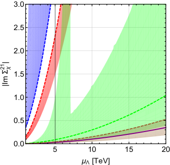
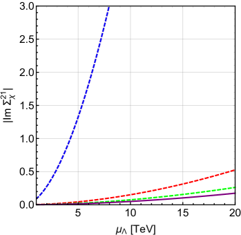
Figure 2: The $|{\rm Im}\,\Sigma^{21}_{\chi}|$ versus the LQ mass ${\mu_{\Lambda}}\sim M_{\rm LQ}$ for fixed $\kappa_{\varepsilon^{\prime}}=0.5$. [Left] for scalar models ${\widetilde{S}}_{1}$ [red], ${\widetilde{R}}_{2}$ [blue], $S_{3}$ [purple], $S_{1}$ [green] and $R_{2}$ [brown]. The bands indicate the variation of $\Sigma^{11}_{L,R}\in[0.0,\,1.0]$ and dashed lines are $\Sigma^{11}_{L,R}=0.0$. [Right] for vector models assuming only EW gauge-mixing: $U_{1,R}$ and $V_{2,L}$ [blue, dashed], $U_{1,L}$ [red, dashed] and $V_{2,R}$ [green, dashed] and $U_{3}$ [purple].

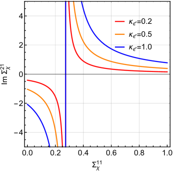
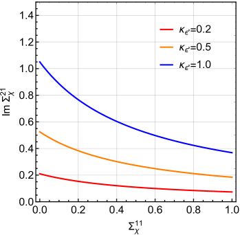
Figure 3: The dependence of the Im$\Sigma^{21}_{L}$ from box contribution $\Sigma^{11}_{R}$ in model $S_{1}$ [left] and $R_{2}$ [right] for different values of $\kappa_{\varepsilon^{\prime}}$ and $M_{\rm LQ}=20$ TeV.

As pointed out above, in other models the box diagrams have a fixed interference behaviour with the EW gauge-mixing term. Therefore a fine-tuned cancellation of the numerically leading contribution from box-diagrams and the EW gauge-mixing term can occur only in the models ${\widetilde{R}}_{2}$ and $S_{1}$ with destructive interference, rendering the subleading terms important. The effect of destructive versus constructive interference on $\mbox{Im}\,\Sigma^{21}_{\chi}$ is depicted in Figure 3 for the two models $S_{1}$ and $R_{2}$, respectively, when varying $\Sigma^{11}_{\chi^{\prime}}\in[0.0,\,1.0]$ for fixed values of $\kappa_{\varepsilon^{\prime}}\neq 0$. In the model $R_{2}$ the constructive interference allows to decrease $\mbox{Im}\,\Sigma^{21}_{\chi}$ with increasing $\Sigma^{11}_{\chi^{\prime}}$, which in turn will lead to smaller effects in other rare Kaon processes that depend only on $\mbox{Im}\,\Sigma^{21}_{\chi}$. On the other hand the destructive interference in model $S_{1}$ leads for intermediate values of $\Sigma^{11}_{\chi^{\prime}}$ to a strong enhancement and sign flip of $\mbox{Im}\,\Sigma^{21}_{\chi}$ in order to maintain a fixed value of $\kappa_{\varepsilon^{\prime}}$ when the expression in parentheses in (4.8) vanishes. In this case rare Kaon processes would receive large contributions.

For the two models ${\widetilde{S}}_{1}$ and ${\widetilde{R}}_{2}$ the dependence of $|\mbox{Im}\,\Sigma^{21}_{\chi}|$ on ${\mu_{\Lambda}}$ is shown in Figure 2 when requiring $\kappa_{\varepsilon^{\prime}}=0.5$ and varying in the box-contribution $\Sigma^{11}_{\chi^{\prime}}\in[0.0,\,1.0]$. The $|\mbox{Im}\,\Sigma^{21}_{\chi}|$ reaches fast a nonperturbative magnitude $>3.0$ to be able to accommodate $\kappa_{\varepsilon^{\prime}}=0.5$, preferring light LQ masses below $8$ TeV as a consequence of the rather small scale in (4.6). Allowing for even larger $\Sigma^{11}_{\chi^{\prime}}$ cannot really ameliorate this situation. In consequence there will be large enhancements of other rare Kaon processes. A similarly low scale is present for sub-scenarios $U_{1,R}$ and $V_{2,L}$ in (4.13). The destructive interference can always lead to a reduction of the effective scale, such that $|\mbox{Im}\,\Sigma^{21}_{\chi}|$ has to become nonperturbative to explain $\kappa_{\varepsilon^{\prime}}=0.5$ for rather low LQ masses. Thus it might be more appropriate to focus on either

1. negligible box contributions,

2. or constructive interference thereby restricting to $\Sigma^{11}_{\chi^{\prime}}<1.0$.

These assumptions should increase the viability of the corresponding scenarios. The results for models $S_{1}$ and $R_{2}$ in Figure 2 show that perturbativity of the couplings is guaranteed even at larger LQ masses $>20$ TeV for suitable choices of $\Sigma^{11}_{\chi^{\prime}}$. Moreover at such high LQ masses, even the constructive interference of the box contributions will reduce the coupling only by a factor of about two compared to the case when they vanish, showing that in these models the consideration of only EW gauge-mixing contributions gives a representative picture for the impact of LQ effects on $(\varepsilon^{\prime}/\varepsilon)_{\rm NP}$.

In the case of vector LQ models $U_{1,3}$ and $V_{2}$ we will use only the EW gauge-mixing contribution in our numerical analysis of the perturbativity of $|\mbox{Im}\,\Sigma^{21}_{\chi}|$ for $\kappa_{\varepsilon^{\prime}}=0.5$. The case of $U_{1}$ and $V_{2}$ is at first sight more involved as having both left-handed and right-handed couplings box contributions to $\varepsilon^{\prime}/\varepsilon$ could be important. In our analysis we will first consider the sub-scenarios with left-handed or right-handed couplings only. In this way potentially large left-right contributions to $\Delta M_{K}$ are absent. The discussion of possible large box contributions to $\varepsilon^{\prime}/\varepsilon$ in these models due to the simultaneous presence of left-handed and right-handed couplings is postponed to Section 5. The results in Figure 2 show that nonperturbativity of the couplings is only an issue for $U_{1,R}$ and $V_{2,L}$.

In our numerical analysis we use analytical formulae and numerical input as given in [21, 24] and described in Section 2.

4.1 Constraints from $K\to\pi\nu\bar{\nu}$

The decays $K_{L}\rightarrow\pi^{0}\nu\bar{\nu}$ and $K^{+}\rightarrow\pi^{+}\nu\bar{\nu}$ provide the most efficient constraints on the combinations (4.1) entering $\varepsilon^{\prime}/\varepsilon$ and apply to the LQ models $S_{1,3}$, ${\widetilde{R}}_{2}$ and $V_{2}$, $U_{1,3}$. We point out that for the model $U_{1}$ with ${\cal C}_{\ell q}^{(1)}={\cal C}_{\ell q}^{(3)}$ at ${\mu_{\Lambda}}$ the first non-vanishing contribution to $K\to\pi\nu\bar{\nu}$ at the scale ${\mu_{\rm ew}}$ via $C_{L}({\mu_{\rm ew}})\propto[{\cal C}_{\ell q}^{(1)}-{\cal C}_{\ell q}^{(3)}]({\mu_{\rm ew}})\propto\alpha_{e}\ln({\mu_{\Lambda}}/{\mu_{\rm ew}}){\cal C}_{\ell q}^{(1)}({\mu_{\Lambda}})$ is due to leading logarithms from gauge mixing and hence loop-suppressed [59]. Still, below we will find that for $\kappa_{\varepsilon^{\prime}}=1.0$ this effect enhances significantly branching ratios for $K_{L}\rightarrow\pi^{0}\nu\bar{\nu}$. As explained in Section 2.2.1 the branching fractions involve a sum over all lepton flavours of the neutrinos in the final state. The LQ contribution in terms of the SMEFT Wilson coefficients at ${\mu_{\rm ew}}$ (3.53) enter as

$$X_{\rm LQ}^{ab} =-s_{W}^{2}v^{2}\frac{\pi}{\alpha_{e}}\frac{\big{[}{\cal C}_{\ell q}^{(1)}-{\cal C}_{\ell q}^{(3)}+{\cal C}_{\ell d}\big{]}_{ba21}}{\lambda_{t}^{sd}},$$ (4.14)

where we will make use of the model-specific relations (3.39) to eliminate ${\cal C}_{\ell q}^{(3)}$. Further, in LQ models the SM$\times$NP term

$$\sum_{a}\mbox{Im}(\lambda_{t}^{sd}X_{\rm LQ}^{aa}) =-s_{W}^{2}v^{2}\frac{\pi}{\alpha_{e}}\sum_{a}\mbox{Im}\big{[}{\cal C}_{\ell q}^{(1)}(1-r_{\rm LQ})+{\cal C}_{\ell d}\big{]}_{aa21}\,,$$ (4.15)

with $r_{\rm LQ}$ given in (3.39), is related to (4.1) entering $\varepsilon^{\prime}/\varepsilon$ since in a particular LQ model only either ${\cal C}_{\ell q}^{(1,3)}$ or ${\cal C}_{\ell d}$ are non-vanishing. Note that here the ${\cal C}_{m}^{(n)}$ are at the scale ${\mu_{\rm ew}}$ whereas in (4.1) at ${\mu_{\Lambda}}$. But for our purpose the self-mixing can be neglected since it is loop-suppressed, such that we equate the Wilson coefficients at both scales.

It is without much loss of generality to assume a hierarchy of the LQ couplings such that a single $[{\cal C}_{m}^{(n)}]_{aa21}\propto g_{1a}^{k\chi}g_{2a}^{k\chi\ast}$ or $\propto h_{2a}^{k\chi}h_{1a}^{k\chi\ast}$ for specific $a=a^{\prime}$ dominates $(\varepsilon^{\prime}/\varepsilon)_{\rm NP}$, in particular one might expect weakest constraints on third-generation lepton couplings of LQs. In consequence, also the SM$\times$NP contribution to ${\cal B}(K_{L}\rightarrow\pi^{0}\nu\bar{\nu})$ will be dominated by this specific coupling and allow for a simple analytic correlation of $\varepsilon^{\prime}/\varepsilon$ and ${\cal B}(K_{L}\rightarrow\pi^{0}\nu\bar{\nu})$. Concerning the NP$\times$NP term, the omission of terms $a\neq b$ in the sum in (2.21) will result always in a lower prediction compared to the true value of ${\cal B}(K_{L}\rightarrow\pi^{0}\nu\bar{\nu})$, i.e. a lower bound on the impact of LQ contributions.

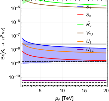
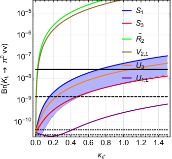
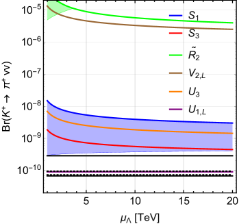
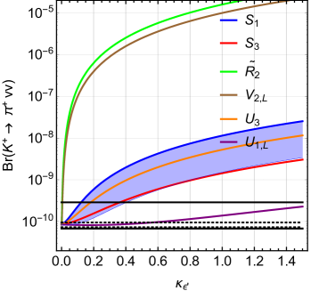
Figure 4: The dependence of ${\cal B}(K_{L}\rightarrow\pi^{0}\nu\bar{\nu})$ [upper] and ${\cal B}(K^{+}\rightarrow\pi^{+}\nu\bar{\nu})$ [lower] on the new physics scale ${\mu_{\Lambda}}\sim M_{\rm LQ}$ for $\kappa_{\varepsilon^{\prime}}=0.5$ [left] and on $\kappa_{\varepsilon^{\prime}}$ for ${\mu_{\Lambda}}=20$ TeV [right], assuming the dominance of a single lepton-flavour coupling that is purely imaginary. For $U_{1,L}$ and $V_{2,L}$, it is assumed that only $L$-LQ couplings are present and saturate $\kappa_{\varepsilon^{\prime}}$. The blue (green) band for $S_{1}$ (${\widetilde{R}}_{2}$) is due to variation of the box-diagrams via $\Sigma_{R(L)}^{11}\in[0.0,\,1.0]$. Further shown are the current upper experimental bound on ${\cal B}(K_{L}\rightarrow\pi^{0}\nu\bar{\nu})$ and the measurement of ${\cal B}(K^{+}\rightarrow\pi^{+}\nu\bar{\nu})$ [73] [black solid], the Grossman-Nir bound from the current measurement of ${\cal B}(K^{+}\rightarrow\pi^{+}\nu\bar{\nu})$ [black dashed] and the SM prediction [21] [black dotted].

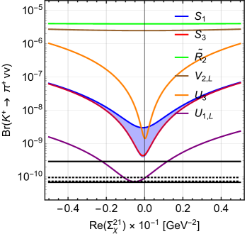
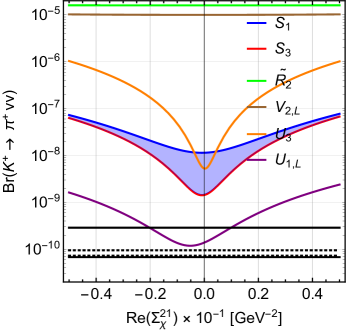
Figure 5: The dependence of ${\cal B}(K^{+}\rightarrow\pi^{+}\nu\bar{\nu})$ on a non-zero real part of the dominant lepton-flavour coupling, for $\kappa_{\varepsilon^{\prime}}=0.5$ [left] and $\kappa_{\varepsilon^{\prime}}=1.0$ [right], with ${\mu_{\Lambda}}=20$ TeV. Further shown are the current measurement of ${\cal B}(K^{+}\rightarrow\pi^{+}\nu\bar{\nu})$ [73] [black solid] and the current SM predictions [21] [black dotted].

With the assumption of the dominance of a single coupling and the requirement that it induces at least a value of $\kappa_{\varepsilon^{\prime}}=0.5$, we can plot ${\cal B}(K_{L}\rightarrow\pi^{0}\nu\bar{\nu})$ vs. ${\mu_{\Lambda}}\in[1,20]$ TeV shown in Figure 4. We set ${\mu_{\rm ew}}=100$ GeV and assume for the moment that box-diagram contributions to $\varepsilon^{\prime}/\varepsilon$ discussed for scalar LQ models in (4.6)–(4.9) are vanishing. The correlation between ${\cal B}(K_{L}\rightarrow\pi^{0}\nu\bar{\nu})$ and $\varepsilon^{\prime}/\varepsilon$ is due to their common dependence on ${\cal C}_{\ell q}^{(1)}$ for $S_{1,3}$, $U_{3}$ or ${\cal C}_{\ell d}$ for ${\widetilde{R}}_{2}$. We show also the correlations in $V_{2,L}$ and $U_{1,L}$ under the assumption that only the $\chi=L$ couplings saturate $\kappa_{\varepsilon^{\prime}}$ via ${\cal C}_{\ell d}$ and ${\cal C}_{\ell q}^{(1)}$, respectively. This assumption is justified for these models as in the presence of both $L$ and $R$ couplings a very strong enhancement of $\Delta M_{K}$ through left-right operators would be possible placing strong constraints on these couplings, despite that box diagrams cannot be calculated reliably without a UV completion.

In general the enhancement of ${\cal B}(K_{L}\rightarrow\pi^{0}\nu\bar{\nu})$ is smaller the larger ${\mu_{\Lambda}}$. The plot shows that for ${\widetilde{R}}_{2}$ and $V_{2,L}$ the ${\cal B}(K_{L}\rightarrow\pi^{0}\nu\bar{\nu})$ will be above the current experimental bound $2.6\times 10^{-8}$ [73] and orders of magnitude above the SM prediction, which excludes these models as an explanation of $\kappa_{\varepsilon^{\prime}}=0.5$. Furthermore the models $S_{1,3}$ and $U_{3}$ give predictions above the Grossman-Nir bound (see Section 2.2.1) and they are almost two orders of magnitude above the SM prediction, thus being also excluded for all practical purposes. We note that it is expected that the final analysis of the 2015 data collected with the KOTO experiment will approach the sensitivity to the Grossman-Nir bound [74]. We plot also ${\cal B}(K_{L}\rightarrow\pi^{0}\nu\bar{\nu})$ versus $\kappa_{\varepsilon^{\prime}}$ for fixed ${\mu_{\Lambda}}=20$ TeV, showing that for larger values of $\kappa_{\varepsilon^{\prime}}$ the enhancement of ${\cal B}(K_{L}\rightarrow\pi^{0}\nu\bar{\nu})$ becomes even more severe. The couplings of the $U_{1,L}$ model enter only via RG effects described in (3.52) and in this case the dependence on ${\mu_{\Lambda}}$ cancels. The enhancement of ${\cal B}(K_{L}\rightarrow\pi^{0}\nu\bar{\nu})\sim 6\,(27)\times 10^{-11}$ is a factor 2 (9) above the SM prediction for $\kappa_{\varepsilon^{\prime}}=0.5\,(1.0)$ and might be tested in the long run of the KOTO experiment.

So far our numerical analysis neglected box-diagram contributions to $\varepsilon^{\prime}/\varepsilon$ presented for scalar LQ models in (4.6)–(4.9). As pointed out there, for the model $S_{3}$ box contributions are suppressed and we expect the same for $U_{3}$. We find for the model $\tilde{R}_{2}$ only enhancement of ${\cal B}(K_{L}\rightarrow\pi^{0}\nu\bar{\nu})$ when varying $\Sigma^{11}_{L}\in[0.0,\,1.0]$, except for small $M_{\rm LQ}\lesssim 4$ TeV, but of negligible size. Box-diagrams in $\varepsilon^{\prime}/\varepsilon$ are more important in model $S_{1}$ as can be seen by the band in Figure 4 that is due to the variation of $\Sigma^{11}_{R}\in[0.0,\,1.0]$. This band shows only how box-diagrams lead to a lowering of ${\cal B}(K_{L}\rightarrow\pi^{0}\nu\bar{\nu})$, but for some values of $\Sigma^{11}_{R}\in[0.0,\,1.0]$ there is also enhancement w.r.t. to the prediction at $\Sigma^{11}_{R}=0$, which is not shown. Going beyond $1.0<\Sigma^{11}_{R}<2.0$ will allow even lower ${\cal B}(K_{L}\rightarrow\pi^{0}\nu\bar{\nu})$, but still ${\cal B}(K_{L}\rightarrow\pi^{0}\nu\bar{\nu})>2\times 10^{-10}$ is about one order of magnitude larger than the SM prediction (2.17) for $\kappa_{\varepsilon^{\prime}}=0.5$.

Despite the additional dependence on real parts of couplings the ${\cal B}(K^{+}\rightarrow\pi^{+}\nu\bar{\nu})$ leads to similar conclusions, which can be expected from the qualitative discussion above. We show the correlation of ${\cal B}(K^{+}\rightarrow\pi^{+}\nu\bar{\nu})$ vs. ${\mu_{\Lambda}}\in[1,20]$ TeV in Figure 4 setting real parts of couplings to zero. The effect of the real couplings is illustrated in Figure 5 for fixed ${\mu_{\Lambda}}=20$ TeV. The models ${\widetilde{R}}_{2}$ (and $V_{2,L}$) and $S_{1}$, $U_{3}$ require ${\cal B}(K^{+}\rightarrow\pi^{+}\nu\bar{\nu})>10^{-9}$, which is at least a factor four above the central value of the current measurement [73], whereas $S_{3}$ is close to the one sigma region. For $\kappa_{\varepsilon^{\prime}}=1.0$, the branching ratios for models in question are all above $10^{-9}$ and excluded, except for $U_{1,L}$, where the enhancement of ${\cal B}(K^{+}\rightarrow\pi^{+}\nu\bar{\nu})$ is very small: a factor 1.1 (1.6) for $\kappa_{\varepsilon^{\prime}}=0.5\,(1.0)$. In the near future the NA62 experiment at CERN will be able to measure ${\cal B}(K^{+}\rightarrow\pi^{+}\nu\bar{\nu})$ with 10% uncertainty at the level of the SM prediction, thus being able to investigate these scenarios further. Also the improved value of $\kappa_{\varepsilon^{\prime}}$ from lattice QCD will be very important here.

4.2 Constraints from $K_{S}\to\mu\bar{\mu}$

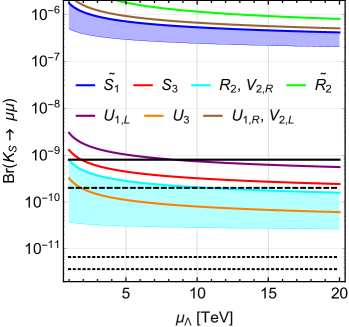
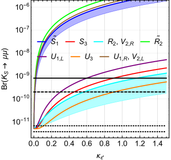
Figure 6: The dependence of ${\cal B}(K_{S}\to\mu\bar{\mu})$ on the new physics scale ${\mu_{\Lambda}}\sim M_{\rm LQ}$ for $\kappa_{\varepsilon^{\prime}}=0.5$ [left] and on $\kappa_{\varepsilon^{\prime}}$ for ${\mu_{\Lambda}}=20$ TeV [right]. For $U_{1}$ and $V_{2}$, it is assumed that either only $L$-LQ or only $R$-LQ couplings are present and saturate $\kappa_{\varepsilon^{\prime}}$. Further shown are the current upper experimental bound on ${\cal B}(K_{S}\to\mu\bar{\mu})$ from LHCb [black solid], a conservative future prospect for LHCb with 23 fb^-1 [black dashed] and the SM prediction [49] [black dotted].

The branching fraction of $K_{S}\to\mu\bar{\mu}$ provides constraints on the muonic LQ couplings in models that generate ${\cal C}_{\ell q}^{(1,3)}$, ${\cal C}_{qe}$, ${\cal C}_{\ell d}$ and ${\cal C}_{ed}$, which are ${\widetilde{S}}_{1}$, $R_{2}$, ${\widetilde{R}}_{2}$, $S_{3}$, $U_{1,3}$ and $V_{2}$. In the LQ model $S_{1}$ no contribution is generated due to EW gauge-mixing (3.51).

Contrary to $K\to\pi\nu\bar{\nu}$, the decay $K_{S}\to\mu\bar{\mu}$ depends only on the muonic LQ couplings, such that a correlation between $\varepsilon^{\prime}/\varepsilon$ and $K_{S}\to\mu\bar{\mu}$ exists only if the muonic LQ couplings were the origin of large $\kappa_{\varepsilon^{\prime}}$. In such a case large NP contributions to (2.31)

$$\frac{\sqrt{{\cal B}(K_{S}\to\mu\bar{\mu})_{\rm SD,NP}}}{(180\,{\rm GeV})^{2}} =\left|{\rm Im}\big{[}{\cal C}_{qe}-{\cal C}_{\ell q}^{(1)}(1+r_{\rm LQ})+{\cal C}_{\ell d}-{\cal C}_{ed}\big{]}_{\mu\mu 21}\right|$$ (4.16)

are correlated with $\varepsilon^{\prime}/\varepsilon$ as can be seen from (4.2). For the convenience of the reader we provide here also the constraints on the SMEFT SL-$\psi^{4}$ Wilson coefficients at ${\mu_{\rm ew}}$ that enter (4.16) when using the experimental bound from LHCb on ${\cal B}(K_{S}\to\mu\bar{\mu})$ (2.32) at 90% C.L.

$$\left|{\rm Im}\big{[}{\cal C}_{qe}-{\cal C}_{\ell q}^{(1)}-{\cal C}_{\ell q}^{(3)}+{\cal C}_{\ell d}-{\cal C}_{ed}\big{]}_{\mu\mu 21}\right|\leq(34\;\mbox{TeV})^{-2}.$$ (4.17)

Following the spirit of [75], it allows easily to set bounds on the imaginary parts when considering one Wilson coefficient at a time.

Considerable simplifications take place in a given LQ model because not all Wilson coefficients are present simultaneously. For example for $S_{3}$, $U_{3}$, $U_{1,L}$ and $R_{2}$ ($r_{R_{2}}=0$) the dominant LQ contribution to $\varepsilon^{\prime}/\varepsilon$ enters via $C_{7}$ as shown in Table 2, such that

$$(\varepsilon^{\prime}/\varepsilon)_{\rm NP} \leq\frac{1.3\times 10^{-4}}{(1+r_{\rm LQ})}\sqrt{\frac{{\cal B}(K_{S}\to\mu\bar{\mu})}{0.8\times 10^{-9}}}\ln\frac{{\mu_{\Lambda}}}{{\mu_{\rm ew}}}.$$ (4.18)

While for ${\mu_{\Lambda}}>10\,{\rm TeV}$, values close to $(\varepsilon^{\prime}/\varepsilon)_{\rm NP}\sim 10^{-3}$ are still allowed, the future improved upper bound on ${\cal B}(K_{S}\to\mu\bar{\mu})$ is likely to lower the upper bound in question below $10^{-4}$.

The dependence of ${\cal B}(K_{S}\to\mu\bar{\mu})$ on ${\mu_{\Lambda}}$ for $\kappa_{\varepsilon^{\prime}}=0.5$ and on $\kappa_{\varepsilon^{\prime}}$ for ${\mu_{\Lambda}}=20$ TeV is shown in Figure 6 assuming the dominance of muonic couplings. Under the latter assumption and requiring $\kappa_{\varepsilon^{\prime}}\geq 0.5$, the current bound on ${\cal B}(K_{S}\to\mu\bar{\mu})$ excludes models ${\widetilde{S}}_{1}$, ${\widetilde{R}}_{2}$, $V_{2,L}$ and $U_{1,R}$ and in part also $U_{1,L}$. The models $S_{3}$, $R_{2}$, $V_{2,R}$ will be all probed with higher statistics at LHCb and one can hope that also $U_{3}$ will be testable [50]. For the models ${\widetilde{S}}_{1}$ and $R_{2}$ the bands show the weakened constraint once allowing for box-diagram contributions to $\varepsilon^{\prime}/\varepsilon$ due to the variation of $\Sigma^{11}_{R,L}\in[0.0,\,1.0]$, respectively, whereas in the model ${\widetilde{R}}_{2}$ they do not weaken the constraint.

Concerning $U_{1}$ and $V_{2}$ models, the bound given above could be in principle eliminated through very high fine-tunning with the help of ${\cal C}_{ed}$ and ${\cal C}_{\ell d}$, respectively. Although they contribute to ${\cal B}(K_{S}\to\mu\bar{\mu})$ without important impact on $\varepsilon^{\prime}/\varepsilon$ where they modify only the coefficients $C_{9}^{\prime}$ and $C_{5}^{\prime}$ the presence of $\chi=L$ and $\chi=R$ couplings of same size are strongly constrained by the bound from $\Delta M_{K}$.

4.3 Constraints from $K_{L}\to\pi^{0}\ell\bar{\ell}$

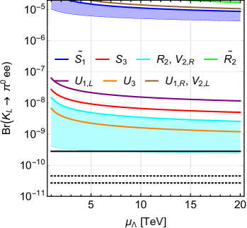
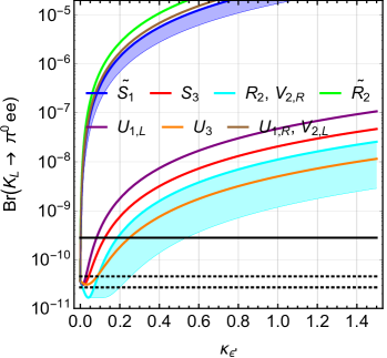
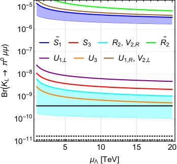
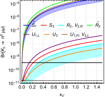
Figure 7: The dependence of ${\cal B}(K_{L}\to\pi^{0}e\bar{e})$ [upper] and ${\cal B}(K_{L}\to\pi^{0}\mu\bar{\mu})$ [lower] on the new physics scale ${\mu_{\Lambda}}\sim M_{\rm LQ}$ for $\kappa_{\varepsilon^{\prime}}=0.5$ [left] and on $\kappa_{\varepsilon^{\prime}}$ for ${\mu_{\Lambda}}=20$ TeV [right], assuming the dominance of the single electronic or muonic lepton-flavour coupling, respectively, that is purely imaginary. For $U_{1}$ and $V_{2}$, it is assumed that either only $L$-LQ or only $R$-LQ couplings are present and saturate $\kappa_{\varepsilon^{\prime}}$. Further shown are the current upper experimental bounds on ${\cal B}(K_{L}\to\pi^{0}\ell\bar{\ell})$ [black solid] and the SM predictions [black dotted].

The branching fractions of $K_{L}\to\pi^{0}e\bar{e}$ and $K_{L}\to\pi^{0}\mu\bar{\mu}$ constrain the electronic and muonic LQ couplings in models that generate ${\cal C}_{\ell q}^{(1,3)}$, ${\cal C}_{qe}$, ${\cal C}_{\ell d}$ and ${\cal C}_{ed}$ at tree-level, which are all models that contribute to $\varepsilon^{\prime}/\varepsilon$, except for $S_{1}$. In contrast to (4.17), no such simple relation can be given here, but allowing one Wilson coefficient to contribute at a time, we find similar bounds for the imaginary parts of all electronic and muonic SL-$\psi^{4}$ Wilson coefficients $a=\{qe,\;\ell q^{(1,3)},\;ed,\;\ell d\}$

$$\left|{\rm Im}[{\cal C}_{a}]_{ee21}\right|\leq(58\;\mbox{TeV})^{-2},$$ (4.19)

$$\left|{\rm Im}[{\cal C}_{a}]_{\mu\mu 21}\right|\leq(50\;\mbox{TeV})^{-2}.$$ (4.20)

For muonic Wilson coefficients this bound is stronger than the bound (4.17) from $K_{S}\to\mu\bar{\mu}$, which is compatible with our analysis that shows that the present constraint from $K_{S}\to\mu\bar{\mu}$ is weaker than from $K_{L}\to\pi^{0}\ell\bar{\ell}$.

The dependence of ${\cal B}(K_{L}\to\pi^{0}e\bar{e})$ and ${\cal B}(K_{L}\to\pi^{0}\mu\bar{\mu})$ on ${\mu_{\Lambda}}$ for $\kappa_{\varepsilon^{\prime}}=0.5$ and on $\kappa_{\varepsilon^{\prime}}$ for ${\mu_{\Lambda}}=20$ TeV is shown in Figure 7 assuming the dominance of electronic and muonic couplings, respectively. These plots are qualitatively analogous to ${\cal B}(K_{S}\to\mu\bar{\mu})$ in Figure 6, but much more stringent due to the stronger experimental bounds on ${\cal B}(K_{L}\to\pi^{0}e\bar{e})$ and ${\cal B}(K_{L}\to\pi^{0}\mu\bar{\mu})$ and in addition also electronic LQ couplings are constrained. All LQ models predict enhancements of ${\cal B}(K_{L}\to\pi^{0}e\bar{e})$ and ${\cal B}(K_{L}\to\pi^{0}\mu\bar{\mu})$ that violate the current bounds once $\kappa_{\varepsilon^{\prime}}\gtrsim 0.5$ for both $\ell=e,\mu$. This demonstrates the importance of both observables in connection with LQ contributions that predict NP to $\varepsilon^{\prime}/\varepsilon$. The only way to avoid these bounds but still to enhance $\varepsilon^{\prime}/\varepsilon$ would be via non-vanishing tauonic LQ couplings, which is ruled out for some LQ models by $K\to\pi\nu\bar{\nu}$ ($S_{1}$, $S_{3}$, $U_{3}$, ${\widetilde{R}}_{2}$ and $V_{2,L}$) and $\Delta M_{K}$ as will be discussed below (${\widetilde{S}}_{1}$, ${\widetilde{R}}_{2}$ and with increasing size of $M_{\rm LQ}$ also $S_{1}$, $S_{3}$ and $R_{2}$).

4.4 Constraints from $\Delta M_{K}$ and $\varepsilon_{K}$

As we have seen the strong correlations between $\varepsilon^{\prime}/\varepsilon$ and $K\to\pi\nu\bar{\nu}$ decays originated in the following features. First in both $\varepsilon^{\prime}/\varepsilon$ and $K\to\pi\nu\bar{\nu}$ a summation over the lepton flavour indices of LQ couplings appears. Second the mutual dependence on the imaginary parts of the couplings. Although the latter applies also to $K_{L}\to\pi^{0}\ell\bar{\ell}$ and $K_{S}\to\mu\bar{\mu}$ decays, the former is absent such that only the electronic and muonic LQ couplings can lead to correlations, whereas tauonic LQ couplings can lift them. In this respect, the off-diagonal elements of the mass-mixing matrix $M_{12}^{sd}$ offer another set of observables that are sensitive to a summation over lepton-flavour indices, as can be seen from the expressions in Appendix C. The relevant observables $\Delta M_{K}$ and $\varepsilon_{K}$ were reviewed in Section 2.3.

As already pointed out in Section 3.7, the LQ contributions to down-type $\Delta F=2$ non-leptonic operators are of different origin then those in $\varepsilon^{\prime}/\varepsilon$. They are actually generated at one-loop at the scale ${\mu_{\Lambda}}$ and provide a loop-suppressed matching contribution with results given in Appendix C for scalar LQ models. But these results involve a summation of products of LQ couplings over the lepton-flavour index, very much as appearing in the sum over the semi-leptonic SMEFT Wilson coefficients entering $\varepsilon^{\prime}/\varepsilon$ in (4.1). Exploiting these model-specific matching results one arrives at

$$C_{\rm VRR}^{sd}({\mu_{\rm ew}}) =\frac{({\cal N}_{sd})^{-1}}{(4\pi)^{2}}\left\{\begin{array}[]{cc}{\displaystyle\frac{M_{{\widetilde{S}}_{1}}^{2}}{2}}\Big{(}\sum_{a}[{\cal C}_{ed}]_{aa21}({\mu_{\Lambda}})\Big{)}^{2}&\qquad\mbox{for}\quad{\widetilde{S}}_{1}\\[11.38092pt] M_{{\widetilde{R}}_{2}}^{2}\Big{(}\sum_{a}[{\cal C}_{\ell d}]_{aa21}({\mu_{\Lambda}})\Big{)}^{2}&\qquad\mbox{for}\quad{\widetilde{R}}_{2}\end{array}\right.$$ (4.23)

where the running from ${\mu_{\Lambda}}$ to ${\mu_{\rm ew}}$ due to self-mixing of ${\cal C}_{dd}$ has been neglected for simplicity. The normalisation factor ${\cal N}_{sd}$ is defined in (2.35). Whereas $\varepsilon^{\prime}/\varepsilon$ is linear in the sum over semi-leptonic Wilson coefficients, $\Delta M_{K}$ and $\varepsilon_{K}$ depend quadratically on it. For LQ models $S_{1,3}$ and $R_{2}$ analogously

$$C_{\rm VLL}^{sd}({\mu_{\rm ew}}) =\frac{({\cal N}_{sd})^{-1}}{(4\pi)^{2}}\left\{\begin{array}[]{cc}2M_{S_{1}}^{2}\Big{(}\sum_{a}[{\cal C}_{\ell q}^{(1)}]_{aa21}({\mu_{\Lambda}})\Big{)}^{2}&\qquad\mbox{for}\quad S_{1}\\[11.38092pt] {\displaystyle\frac{M_{R_{2}}^{2}}{2}}\Big{(}\sum_{a}[{\cal C}_{qe}]_{aa21}({\mu_{\Lambda}})\Big{)}^{2}&\qquad\mbox{for}\quad R_{2}\\[14.22636pt] {\displaystyle\frac{10}{9}}M_{S_{3}}^{2}\Big{(}\sum_{a}[{\cal C}_{\ell q}^{(1)}]_{aa21}({\mu_{\Lambda}})\Big{)}^{2}&\qquad\mbox{for}\quad S_{3}\end{array}\right.$$ (4.27)

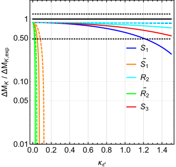
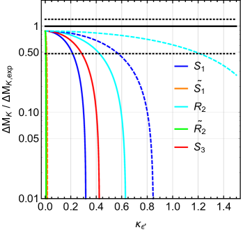
Figure 8: The dependence of the short-distance part of $\Delta M_{K}/\Delta M_{K,{\rm exp}}$ on $\kappa_{\varepsilon^{\prime}}$ for $M_{\rm LQ}=2$ TeV [left] and $M_{\rm LQ}=20$ TeV [right]. The dashed lines show the effect of box-diagram contributions in $\varepsilon^{\prime}/\varepsilon$ for $\Sigma^{11}_{L,R}\in[0.0,\,1.0]$. Further shown are the experimental measurement [black solid] and the SM prediction [black dotted].

For example the correlation between $\kappa_{\varepsilon^{\prime}}$ and $\Delta M_{K}$ takes the form

$$\frac{(\Delta M_{K})^{\rm LQ}}{(\Delta M_{K})^{\rm exp}} =-1.3\,\left(\frac{\kappa_{\varepsilon^{\prime}}}{\ln({\mu_{\Lambda}}/{\mu_{\rm ew}})}\,\frac{M_{\rm LQ}}{2\,{\rm TeV}}\right)^{2}$$ (4.28)

in the $S_{3}$ model in which $C_{7}$ dominates the NP contribution to $\varepsilon^{\prime}/\varepsilon$. It should be noted that suppression of $\Delta M_{K}$ by the LQ contribution increases with increasing $M_{\rm LQ}$, a feature found already in [20] in the context of $Z^{\prime}$ models. This shows that $\Delta M_{K}$ can provide powerful constraints on scalar LQ models, even though numerically enhanced left-right operators do not contribute.

The strong correlation of $\varepsilon^{\prime}/\varepsilon$ and the short-distance part of $\Delta M_{K}$ is specific for each LQ model and shown in Figure 8 for $M_{\rm LQ}=2,\,20$ TeV. The LQ models ${\widetilde{S}}_{1}$ and ${\widetilde{R}}_{2}$ lead even for very small $\kappa_{\varepsilon^{\prime}}\lesssim 0.05$ to a strong decrease by orders of magnitude independently of $M_{\rm LQ}$. The correlation of $\varepsilon^{\prime}/\varepsilon$ and $\Delta M_{K}$ can be dampened for low $M_{\rm LQ}$ of a few TeV in models $S_{1,3}$ and $R_{2}$, but at large scales $M_{\rm LQ}\gtrsim 10$ TeV again strong suppression of $\Delta M_{K}$ for $\kappa_{\varepsilon^{\prime}}\gtrsim 0.3$ sets in disfavouring them as a explanation of $\varepsilon^{\prime}/\varepsilon$, with weakest constraints on the model $R_{2}$. At this point strictly imaginary couplings were assumed. In Figure 9 we show the impact of small real contributions to the couplings on $\Delta M_{K}$ and $\varepsilon_{K}$ for $\kappa_{\varepsilon^{\prime}}=0.5$ and $M_{\rm LQ}=2,\,20$ TeV. Although it seems that fine-tuning between real and imaginary parts can bring $\Delta M_{K}$ in agreement with data, actually $\varepsilon_{K}$ becomes changed by orders of magnitude, even for $M_{\rm LQ}$ of a few TeV. On the other hand the presence of box-diagram contributions in $\varepsilon^{\prime}/\varepsilon$ can further weaken the constraints from $\Delta M_{K}$, but at the same time are subject to constraints from $D^{0}-{\overline{D}}^{0}$ mixing, which are sensitive to left-right operators.

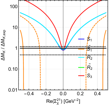
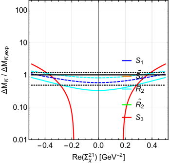
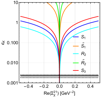
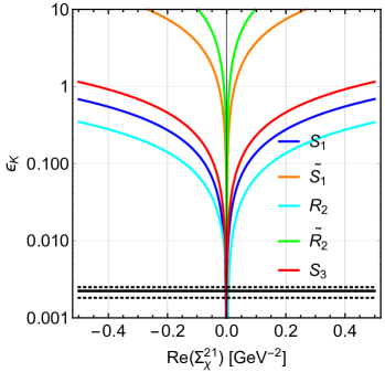
Figure 9: The dependence of the short-distance part of $\Delta M_{K}/\Delta M_{K,{\rm exp}}$ [upper] and $\varepsilon_{K}$ [lower] on real parts of couplings for $M_{\rm LQ}=2$ TeV [left] and $M_{\rm LQ}=20$ TeV [right] for $\kappa_{\varepsilon^{\prime}}=0.5$. Further shown are the experimental measurement [black solid] and the SM prediction [black dotted].

While no reliable calculations of $\Delta M_{K}$ and $\varepsilon_{K}$ can be performed in models with vector LQs without invoking a UV completion we would like to make an observation on the models $U_{1}$ and $V_{2}$, which will turn out to be relevant soon. As seen in (A.2) in these models two couplings with $\chi=L$ and $\chi^{\prime}=R$ are present. If both are non-zero, strongly enhanced left-right operators contributing to $\Delta M_{K}$ and $\varepsilon_{K}$ will be present. In fact the chiral enhancement of the hadronic matrix elements of such operators combined with RG evolution brings in an enhancement of these contributions by two orders of magnitude relative to VLL and VRR cases [24] constraining strongly this model in the presence of large imaginary couplings. Thus one might set one of the two couplings to zero, what we have done while presenting the numerical results above. We expect therefore strong constraints from $\Delta M_{K}$ and $\varepsilon_{K}$ on the couplings of these models even without this approximation.

5 Summary, Conclusions and Outlook

In this paper we have presented for the first time the analysis of $\varepsilon^{\prime}/\varepsilon$ in LQ models and provided general formulae in the framework of SMEFT for models in which non-leptonic operators governing $\varepsilon^{\prime}/\varepsilon$ are generated from semi-leptonic operators through electroweak (EW) renormalisation group (RG) effects. We have also performed the one-loop decoupling for scalar LQ models.

Our analysis showed the strong correlation of rare Kaon processes with $\varepsilon^{\prime}/\varepsilon$. They imply strong constraints on LQ models from the rare Kaon sector in the case of a future confirmation of the $\varepsilon^{\prime}/\varepsilon$ anomaly by lattice QCD. They can be further strengthened with improved measurements of $K^{+}\rightarrow\pi^{+}\nu\bar{\nu}$ by NA62, $K_{L}\rightarrow\pi^{0}\nu\bar{\nu}$ by KOTO and $K_{S}\to\mu\bar{\mu}$ by LHCb, as well as a improved lattice result for $\Delta M_{K}$ in the Standard Model (SM). Hopefully also $K_{L}\to\pi^{0}\ell\bar{\ell}$ decays will one day help in this context. Within our approximations, we were able to consider most relevant contributions to $\varepsilon^{\prime}/\varepsilon$ from EW gauge-mixing for both scalar and vector LQ models, and from one-loop decoupling in a complete manner for scalar LQ models. On the one hand, the EW gauge-mixing generates numerically enhanced EW-penguin operator $Q_{7}$ in models $S_{1,3}$, $R_{2}$, $U_{1,L}$, $V_{2,R}$ and $U_{3}$. On the other hand, the box-diagram contributions exhibit in LQ models with left-handed and right-handed couplings ($S_{1}$, $R_{2}$, $U_{1}$ and $V_{2}$) the remarkable feature that they can generate EW-penguin operators $Q_{8,8^{\prime}}$ already at the LQ scale. In turn they are numerically strongly enhanced in $\varepsilon^{\prime}/\varepsilon$ through RG effects and their hadronic matrix elements. Notably, the latter contributions involve both LQ couplings of the corresponding models and would vanish if either of them were zero. The main results of our analysis might be summarised as follows

• The models with only one LQ coupling ${\widetilde{S}}_{1}$, ${\widetilde{R}}_{2}$, $S_{3}$ and $U_{3}$ lead to large enhancement of the branching fractions of $K_{L}\rightarrow\pi^{0}\nu\bar{\nu}$ and $K^{+}\rightarrow\pi^{+}\nu\bar{\nu}$ if $(\varepsilon^{\prime}/\varepsilon)_{\rm NP}$ is non-vanishing, such that for moderate enhancements $\kappa_{\varepsilon^{\prime}}=0.5$ the current bounds on both decays exclude these models as a possible explanation of the $\varepsilon^{\prime}/\varepsilon$ anomaly. Here the box-diagram contributions to $\varepsilon^{\prime}/\varepsilon$ have been included, thereby assuming the involved couplings to stay perturbative. We expect that even going beyond this assumption will be in general insufficient to explain the $\varepsilon^{\prime}/\varepsilon$ anomaly, even for the vector LQ model $U_{3}$, where we are not able to calculate box diagrams in a cut-off independent manner without specifying a UV completion.

• The model $S_{1}$ shows also strong enhancement of $K_{L}\rightarrow\pi^{0}\nu\bar{\nu}$ and $K^{+}\rightarrow\pi^{+}\nu\bar{\nu}$ above the current Grossman-Nir bound even when box-diagram contributions are included as long as $\Sigma^{11}_{R}<1.0$, but for larger values of $\Sigma^{11}_{R}$ a stronger bound on $K_{L}\rightarrow\pi^{0}\nu\bar{\nu}$ and $K^{+}\rightarrow\pi^{+}\nu\bar{\nu}$ is required to conclusively exclude it as an explanation of the $\varepsilon^{\prime}/\varepsilon$ anomaly.

• The sub-scenario of vector LQ model $V_{2,L}$ predicts also huge enhancements of $K_{L}\rightarrow\pi^{0}\nu\bar{\nu}$ and $K^{+}\rightarrow\pi^{+}\nu\bar{\nu}$ for $\kappa_{\varepsilon^{\prime}}\gtrsim 0.1$ if only EW gauge-mixing is included in $\varepsilon^{\prime}/\varepsilon$. From our experience with $\tilde{R}_{2}$ we expect that the inclusion of box-diagrams to $\varepsilon^{\prime}/\varepsilon$ will not be able to avoid this strong enhancement, leaving $V_{2,L}$ as a very unlikely explanation of the $\varepsilon^{\prime}/\varepsilon$ anomaly.

• For the other models $R_{2}$, $U_{1,L}$, $U_{1,R}$ and $V_{2,R}$ we see large enhancements in $K_{S}\to\mu\bar{\mu}$ and $K_{L}\to\pi^{0}\ell\bar{\ell}$, which put stringent constraints on electron and muon couplings and hence on the LQ parameter space. But tauonic LQ couplings remain unconstrained and can serve as an explanation of $\varepsilon^{\prime}/\varepsilon$. In the scalar LQ model $R_{2}$ this statement includes box-diagram contributions to $\varepsilon^{\prime}/\varepsilon$ with $\Sigma^{11}_{R}<1.0$.

• For the scalar LQ models $S_{1}$ and $R_{2}$ the box-diagrams for $\Delta F=2$ processes are calculable and here $\Delta M_{K}$ provides complementary bounds also on tauonic LQ couplings, but their effectivity becomes weak with smaller LQ masses for the case of purely imaginary $\Sigma^{21}_{\chi}$. If $\Sigma^{21}_{\chi}$ has also a small real part then $\Delta M_{K}$ and also $\varepsilon_{K}$ become powerful constraints on large deviations in $\varepsilon^{\prime}/\varepsilon$ from the SM.

The LQ models which have the best chance to explain the $\varepsilon^{\prime}/\varepsilon$ anomaly are then the scalar LQ models $R_{2}$ and in part $S_{1}$ and two vector LQ models $U_{1}$ and $V_{2}$. Among these four models only the model $U_{1}$ has a chance to explain the $B$ physics anomalies if only one LQ representation is considered. But as suggestions have been made to explain $B$ physics anomalies by considering simultaneously two LQ representations [7, 8, 6] and $B$ physics anomalies could disappear one day we analysed all these models.

We have pointed out that in models $R_{2}$ and $S_{1}$ the large contribution to $\varepsilon^{\prime}/\varepsilon$ via box-diagrams (3.48) involves both couplings $\sim\Sigma^{21}_{\chi}\Sigma^{11}_{\chi^{\prime}}$ with $\chi\neq\chi^{\prime}$. A similar combination $\sim V_{m2}V_{n1}^{\ast}\,\Sigma^{mn}_{\chi}\Sigma^{21}_{\chi^{\prime}}$ can be bounded in principle by $D^{0}-{\overline{D}}^{0}$ mixing, providing also constraints on the tauonic LQ couplings. Indeed it is well known that LR operators have enhanced matrix elements not only for $K^{0}-{\overline{K}}^{0}$ mixing, but also for $D^{0}-{\overline{D}}^{0}$ mixing [76, 77]. However, due to the presence of the quark-mixing matrix $V$ only a detailed global analysis can provide a conclusive answer how strong $D^{0}-{\overline{D}}^{0}$ mixing can constrain box-diagram contributions to $\varepsilon^{\prime}/\varepsilon$. Such an analysis is beyond the scope of our paper.

In vector LQ models $U_{1}$ and $V_{2}$ the $\Delta F=2$ constraints will be even stronger since here LR operators contribute to $\Delta M_{K}$ and $\varepsilon_{K}$, where they are strongly enhanced, see [24] for recent updates. The box-diagrams contribute to $\varepsilon^{\prime}/\varepsilon$ via the EW-penguin operator $Q_{8}$ (and also $Q_{8^{\prime}}$, but with Cabibbo suppression) (3.49) involving the combinations $\sim\Sigma^{21}_{\chi}\Sigma^{11}_{\chi^{\prime}}$ with $\chi\neq\chi^{\prime}$, whereas $\Delta F=2$ observables depend on $\sim\Sigma^{21}_{\chi}\Sigma^{21}_{\chi^{\prime}}$. Again tauonic couplings are in principle also subject to constraints, but similar to scalar LQ models, also here only a global analysis on the basis of a UV completion can provide a conclusive answer on the effectivity of these constraints.

Whether the LQ models where the $\varepsilon^{\prime}/\varepsilon$ anomaly seems to be still compatible with present constraints from rare Kaon processes are challenged by other existing constraints goes beyond the scope of our work. This would require dedicated global analysis of each model. In the case of vector LQ models a UV completion should be considered, as for example proposed in [78, 10, 9, 79]. These UV completions contain usually new gauge and scalar sectors, subject to additional constraints beyond flavour physics. On the other hand, UV completions based on models with partial compositeness [80] or composite Higgs models [81, 82] also lack full predictability due to the strongly interacting dynamics in these models, requiring nonperturbative methods. We conclude therefore that the inclusion of box-diagram contributions to $\varepsilon^{\prime}/\varepsilon$ with both left-handed and right-handed couplings can improve the situation in models $R_{2}$, $S_{1}$, $V_{2}$ and $U_{1}$ but this improvement might be insufficient to explain the $\varepsilon^{\prime}/\varepsilon$ anomaly in LQ models, in particular if $\kappa_{\varepsilon^{\prime}}$ will turn out to be close to unity.

It should also be emphasized that the presence of significant right-handed couplings goes against the present wisdom based on $B$ physics anomalies that new physics is dominated by left-handed currents, see in particular [8]. But as the $U_{1}$ model is favoured by $B$ physics anomalies our analysis challenges model builders to find a UV completion for this model that includes also right-handed couplings and couplings to the first generation and while explaining the $\varepsilon^{\prime}/\varepsilon$ anomaly, satisfies all existing constraints, in particular describes $B$ physics anomalies and is consistent with the bounds on $\Delta M_{K}$ and $\varepsilon_{K}$ that are very strong in the presence of left-handed and right-handed couplings.

While the vector LQ $U_{1}$ performs best as a single representation in the case of $B$-physics anomalies, models with two or more LQ representations have been considered in the literature in the context of these anomalies. The question then arises whether with two LQ representations the results for $\varepsilon^{\prime}/\varepsilon$ would improve. We comment here briefly on two such models with scalar LQs, one involving $S_{1}$ and $S_{3}$ representations [7, 8] and the second $S_{3}$ and $\tilde{R}_{2}$ representations [6].

$S_{1}$

${\widetilde{S}}_{1}$

$R_{2}$

${\widetilde{R}}_{2}$

$S_{3}$

$U_{1,L}$

$U_{1,R}$

$U_{1}$

$V_{2,L}$

$V_{2,R}$

$V_{2}$

$U_{3}$

$K_{L}\rightarrow\pi^{0}\nu\bar{\nu}$

$\dagger$

—

—

$\dagger$

$\dagger$

—

$\dagger$

—

$\dagger$

$K^{+}\rightarrow\pi^{+}\nu\bar{\nu}$

$\dagger$

—

—

$\dagger$

$\dagger$

—

$\dagger$

—

$\dagger$

$K_{L}\to\pi^{0}\ell\bar{\ell}$

—

$\dagger_{e,\mu}$

$\dagger_{e,\mu}$

$\dagger_{e,\mu}$

$\dagger_{e,\mu}$

$\dagger_{e,\mu}$

$\dagger_{e,\mu}$

$\dagger_{e,\mu}$

$\dagger_{e,\mu}$

$\dagger_{e,\mu}$

$K_{S}\to\mu\bar{\mu}$

—

$\dagger_{\mu}$

$\dagger_{\mu}$

$\dagger_{\mu}$

$\dagger_{\mu}$

$\Delta M_{K}$, $\varepsilon_{K}$

$\dagger_{\mu_{\Lambda}}$

$\dagger$

$\dagger$

$\dagger_{\mu_{\Lambda}}$

loop

loop

loop

loop

loop

loop

loop

$\sum$

$\dagger$

$\dagger$

$\dagger_{e,\mu}$

$\dagger$

$\dagger$

$\dagger_{e,\mu}$

$\dagger_{e,\mu}$

$\dagger$

$\dagger_{e,\mu}$

$\dagger$

Table 3: Overview of strong conflicts with current bounds/measurements on rare Kaon processes when requiring $(\varepsilon^{\prime}/\varepsilon)_{\rm NP}=\kappa_{\varepsilon^{\prime}}\times 10^{-3}$ with $\kappa_{\varepsilon^{\prime}}\gtrsim 0.5$ for scalar and vector LQ models. In vector LQ models only the EW gauge-mixing is included in $\varepsilon^{\prime}/\varepsilon$, see main text for details. The symbols in the table correspond to: “—” = no contributions in this LQ model; “loop” = mediated by loop corrections in vector LQ models; “$\dagger$” = ruled out for all lepton flavours $\ell=e,\mu,\tau$; “$\dagger_{\ell}$” = ruled out for lepton flavour $\ell$; “$\dagger_{\mu_{\Lambda}}$” = ruled out for all lepton flavour if LQ mass is large enough.

Looking at (4.7) and (4.8) we observe that in the case of a model with $S_{1}$ and $S_{3}$ the value of the coupling $\Sigma_{\chi,\text{LQ}}^{sd}$ can be decreased for a given $\kappa_{\varepsilon^{\prime}}$. Assuming that the couplings in these two representations are equal the coupling in question can be decreased by a factor 1.33 implying the reduction of the branching ratio for $K_{L}\rightarrow\pi^{0}\nu\bar{\nu}$ in the case of $S_{3}$ model first by a factor 1.8 with a smaller effect in $K^{+}\rightarrow\pi^{+}\nu\bar{\nu}$. But as in both cases now also $S_{1}$ contributes the change is smaller. While this still improves the situation the model is still predicting values of $\mathcal{B}(K_{L}\rightarrow\pi^{0}\nu\bar{\nu})$ close to the Grossman-Nir bound and similar comments apply to $K^{+}\rightarrow\pi^{+}\nu\bar{\nu}$ where the change is smaller. In the case of $K_{L}\to\pi^{0}\ell\bar{\ell}$ the representation $S_{1}$ does not contribute and one can see by inspecting Figure 7 that this reduction of the coupling and of the branching ratio does not really solve the problem.

As far as combination of $S_{3}$ and $\tilde{R}_{2}$ is concerned the great disparity in the effectiveness of these two representations to enhance $\varepsilon^{\prime}/\varepsilon$ seen in (4.6) and (4.7) tells us that the results of the $S_{3}$ model remain practically unchanged. These two examples indicate that even invoking more representations it will be difficult to enhance sufficiently $\varepsilon^{\prime}/\varepsilon$, in particular if $\kappa_{\varepsilon^{\prime}}$ close to unity will be required.

The goal of our paper was to demonstrate on the basis of Kaon physics alone that the explanation of a possible $\varepsilon^{\prime}/\varepsilon$ anomaly within the context of LQ models was very unlikely. Any additional constraint on the couplings of LQs would further strengthen this conclusion. Such constraints could come in particular from $B$ physics anomalies but this would require the imposition of flavour symmetries that would relate $K$ and $B$ decays. In connection with the latter it has been demonstrated in [83] that the imposition of minimal flavour violation (MFV) on LQ models excludes the explanation of $B$ physics anomalies within these models. We would like to emphasize that in the case of $\varepsilon^{\prime}/\varepsilon$ MFV is broken from the beginning as only significant new CP-violating phases have a chance to explain the anomaly in question.

Another possible constraint could come from the simultaneous considerations of flavour symmetries responsible from the observed spectrum of fermion masses. In the context of $B$ physics anomalies this issue has been addressed in [80] for the scalar LQ model $S_{3}$ in the framework of partial compositeness and for ${\widetilde{R}}_{2}$ and $S_{3}$ models imposing various flavour symmetries in [84]. Our analysis shows that in these frameworks the bounds on $K_{L}\rightarrow\pi^{0}\nu\bar{\nu}$ and $K^{+}\rightarrow\pi^{+}\nu\bar{\nu}$ are violated when requiring $\kappa_{\varepsilon^{\prime}}\geq 0.05$ for ${\widetilde{R}}_{2}$ and $\kappa_{\varepsilon^{\prime}}\geq 0.4$ for $S_{3}$. It will be interesting to generalize such studies to include $\varepsilon^{\prime}/\varepsilon$ and in particular $K^{+}\rightarrow\pi^{+}\nu\bar{\nu}$ after the result from NA62 will be known. In case $\varepsilon^{\prime}/\varepsilon$ and $B$ physics anomalies would persist and the measurement of the $K^{+}\rightarrow\pi^{+}\nu\bar{\nu}$ branching ratio would significantly deviate from the rather precise SM prediction, a valuable information on family structure of BSM models could be obtained. We hope to return to this issue once the $\varepsilon^{\prime}/\varepsilon$ anomaly will be confirmed and the experimental status of $B$ physics anomalies and of $K^{+}\rightarrow\pi^{+}\nu\bar{\nu}$ will improve.

Our findings for the ten LQ models listed in Table 4 as far as the $\varepsilon^{\prime}/\varepsilon$ anomaly in correlation with rare Kaon processes is concerned are summarised in Table 3 The different symbols appearing in this table are explained in the caption of this table.

Finally, in most papers analysing LQ and other models in the context of $B$ physics anomalies it is a common practice to set NP couplings to Kaon and other light physics sectors to zero. If the $\varepsilon^{\prime}/\varepsilon$ anomaly will be confirmed by future lattice results all these analyses have to be reconsidered.

The main messages of our analysis to take home are the following ones. If the future improved lattice calculation will confirm the $\varepsilon^{\prime}/\varepsilon$ anomaly at the level $(\varepsilon^{\prime}/\varepsilon)_{\rm NP}\geq 5\times 10^{-4}$ LQs are likely not responsible for it. But if the $\varepsilon^{\prime}/\varepsilon$ anomaly will disappear one day, large NP effects in rare $K$ decays that are still consistent with present bounds will be allowed.

Appendix A LQ Lagrangian

Here we summarise our conventions for the LQ Lagrangian, which follows [1]. The transformation properties of the spin $S=0$ (scalar) and $S=1$ (vector) LQ’s under the SM group ${\mathrm{G_{SM}}}\equiv{\mathrm{SU(3)_{c}}}\otimes{\mathrm{SU(2)_{L}}}\otimes{\mathrm{U(1)_{Y}}}$ are summarised in Table 4. We have modified the definition of the ${\mathrm{SU(2)_{L}}}$ doublet LQ’s $R_{2}$, ${\widetilde{R}}_{2}$ and $V_{2}$, ${\widetilde{V}}_{2}$ to follow the standard conventions for quark, lepton and Higgs doublets in which upper and lower ${\mathrm{SU(2)_{L}}}$ components correspond to isospin $+1/2$ and $-1/2$, respectively, opposite to the original convention in [1].

LQ	$S_{1}$	${\widetilde{S}}_{1}$	$R_{2}$	${\widetilde{R}}_{2}$	$S_{3}$	$U_{1}$	${\widetilde{U}}_{1}$	$V_{2}$	${\widetilde{V}}_{2}$	$U_{3}$
${\mathrm{SU(3)_{c}}}$	$3^{\ast}$	$3^{\ast}$	$3\;\;$	$3\;\;$	$3^{\ast}$	$3\;\;$	$3\;\;$	$3^{\ast}$	$3^{\ast}$	$3$
${\mathrm{SU(2)_{L}}}$	$1\;$	$1\;$	$2\;\;$	$2\;\;$	$3\;$	$1\;\;$	$1\;\;$	$2\;\,$	$2\;\,$	$3$
${\mathrm{U(1)_{Y}}}$	$2/3$	$8/3$	$7/3$	$1/3$	$2/3$	$4/3$	$10/3$	$5/3$	$-1/3$	$4/3$
$T_{3}$	$0$	$0$	$\begin{array}[]{cc}+\frac{1}{2}\\ -\frac{1}{2}\end{array}$	$\begin{array}[]{cc}+\frac{1}{2}\\ -\frac{1}{2}\end{array}$	$\begin{array}[]{cc}+1\\ 0\\ -1\end{array}$	$0$	$0$	$\begin{array}[]{cc}+\frac{1}{2}\\ -\frac{1}{2}\end{array}$	$\begin{array}[]{cc}+\frac{1}{2}\\ -\frac{1}{2}\end{array}$	$\begin{array}[]{cc}+1\\ 0\\ -1\end{array}$
$Q_{\rm em}$	$1/3$	$4/3$	$\begin{array}[]{cc}5/3\\ 2/3\end{array}$	$\begin{array}[]{cc}+2/3\\ -1/3\end{array}$	$\begin{array}[]{cc}+4/3\\ +1/3\\ -2/3\end{array}$	$2/3$	$5/3$	$\begin{array}[]{cc}4/3\\ 1/3\end{array}$	$\begin{array}[]{cc}+1/3\\ -2/3\end{array}$	$\begin{array}[]{cc}+5/3\\ +2/3\\ -1/3\end{array}$

Table 4: Quantum numbers of LQ’s under the gauge groups of the SM, and the isospin $T_{3}$ and electric charge $Q_{\rm em}$ of their ${\mathrm{SU(2)_{L}}}$ components, $Q_{\rm em}=T_{3}+Y/2$.

The couplings of scalar LQs to quarks ($q_{L},u_{R},d_{R}$) and leptons ($\ell_{L},e_{R}$) in the unbroken ${\mathrm{SU(2)_{L}}}\otimes{\mathrm{U(1)_{Y}}}$ phase are

$${\cal L}_{S} =\left(g^{1L}\left[{\overline{q^{c}_{L}}}i\tau^{2}\ell_{L}\right]+g^{1R}\left[{\overline{u^{c}_{R}}}e_{R}\right]\right)S_{1}+\widetilde{g}^{1R}\left[{\overline{d^{c}_{R}}}e_{R}\right]{\widetilde{S}}_{1}$$ (A.1)

$$+h^{2L}\left[{\overline{u}}_{R}R_{2}^{T}i\tau^{2}\ell_{L}\right]+h^{2R}\left[{\overline{q}}_{L}R_{2}e_{R}\right]+\widetilde{h}^{2L}\left[{\overline{d}}_{R}{\widetilde{R}}_{2}^{T}i\tau^{2}\ell_{L}\right]$$

$$+g^{3L}\left[{\overline{q^{c}_{L}}}i\tau^{2}\vec{\bm{\tau}}\ell_{L}\right]\bm{\cdot\,\vec{S}_{3}}+\,\mbox{h.c.},$$

and for vector LQs

$${\cal L}_{V} =\left(h^{1L}\left[{\overline{q}}_{L}\gamma_{\mu}\ell_{L}\right]+h^{1R}\left[{\overline{d}}_{R}\gamma_{\mu}e_{R}\right]\right)U_{1}^{\mu}+\widetilde{h}^{1R}\left[{\overline{u}}_{R}\gamma_{\mu}e_{R}\right]{\widetilde{U}}_{1}^{\mu}$$ (A.2)

$$+g^{2L}\left[{\overline{d^{c}_{R}}}\gamma_{\mu}(V_{2}^{\mu})^{T}i\tau^{2}\ell_{L}\right]+g^{2R}\left[{\overline{q^{c}_{L}}}\gamma_{\mu}i\tau^{2}V_{2}^{\mu}e_{R}\right]+\widetilde{g}^{2L}\left[{\overline{u^{c}_{R}}}\gamma_{\mu}({\widetilde{V}}_{2}^{\mu})^{T}i\tau^{2}\ell_{L}\right]$$

$$+h^{3L}\left[{\overline{q}}_{L}\gamma_{\mu}\vec{\bm{\tau}}\ell_{L}\right]\bm{\cdot\,\vec{U}_{3}^{\mu}}+\,\mbox{h.c.}$$

where the generation indices on quark and lepton fields have been suppressed. The LQ couplings $g^{a\chi}$, ${\widetilde{g}}^{a\chi}$ and $h^{a\chi}$, ${\widetilde{h}}^{a\chi}$ ($a=1,2,3$ and $\chi=L,R$) are $3\times 3$ complex-valued matrices in the generation space of the quarks and leptons. Above $(i\tau^{2})_{ab}=\varepsilon_{ab}$ is the second Pauli matrix, $\varepsilon_{12}=-\varepsilon_{21}=+1$. Charge-conjugated fields are denoted as $\psi^{c}\equiv C{\overline{\psi}}^{T}$ with the charge-conjugation matrix $C$.

Appendix B LQ tree-level decoupling

The tree-level decoupling of LQs gives rise to semi-leptonic operators in SMEFT. Here we summarise the results of their Wilson coefficients at the LQ scale ${\mu_{\Lambda}}$. The semi-leptonic operators are listed in Table 1. There are two classes of diagrams to consider, depending on whether charge-conjugated fields are involved or not. We follow [85] for Feynman rules and consider the tree-level matching for $Q_{i}+L_{a}\to Q_{j}+L_{b}$.

$$S_{1} : [{\cal C}_{\ell q}^{(1)}]_{baji}=-[{\cal C}_{\ell q}^{(3)}]_{baji} =\frac{g^{1L}_{ia}g^{1L\ast}_{jb}}{4M^{2}},$$ (B.1)

$$[{\cal C}_{eu}]_{baji} =\frac{g^{1R}_{ia}g^{1R\ast}_{jb}}{2M^{2}},$$ (B.2)

$$[{\cal C}_{\ell equ}^{(1)}]_{abij}^{\ast}=-4[{\cal C}_{\ell equ}^{(3)}]_{abij}^{\ast} =\frac{g^{1L}_{ia}g^{1R\ast}_{jb}}{2M^{2}},$$ (B.3)

$${\widetilde{S}}_{1} : [{\cal C}_{ed}]_{baji} =\frac{{\widetilde{g}}^{1R}_{ia}{\widetilde{g}}^{1R\ast}_{jb}}{2M^{2}},$$ (B.4)

$$R_{2} : [{\cal C}_{\ell u}]_{baji} =-\frac{h^{2L}_{ja}h^{2L\ast}_{ib}}{2M^{2}},$$ (B.5)

$$[{\cal C}_{qe}]_{baji} =-\frac{h^{2R}_{ja}h^{2R\ast}_{ib}}{2M^{2}},$$ (B.6)

$$[{\cal C}_{\ell equ}^{(1)}]_{abij}^{\ast}=4[{\cal C}_{\ell equ}^{(3)}]_{abij}^{\ast} =\frac{h^{2L}_{ja}h^{2R\ast}_{ib}}{2M^{2}},$$ (B.7)

$${\widetilde{R}}_{2} : [{\cal C}_{\ell d}]_{baji} =-\frac{{\widetilde{h}}^{2L}_{ja}{\widetilde{h}}^{2L\ast}_{ib}}{2M^{2}},$$ (B.8)

$$S_{3} : [{\cal C}_{\ell q}^{(1)}]_{baji}=3[{\cal C}_{\ell q}^{(3)}]_{baji} =\frac{3}{4}\frac{g^{3L}_{ia}g^{3L\ast}_{jb}}{M^{2}},$$ (B.9)

$$U_{1} : [{\cal C}_{\ell q}^{(1)}]_{baji}=[{\cal C}_{\ell q}^{(3)}]_{baji} =-\frac{h^{1L}_{ja}h^{1L\ast}_{ib}}{2M^{2}},$$ (B.10)

$$[{\cal C}_{ed}]_{baji} =-\frac{h^{1R}_{ja}h^{1R\ast}_{ib}}{M^{2}},$$ (B.11)

$$[{\cal C}_{\ell edq}]_{abij}^{\ast} =2\frac{h^{1L}_{ja}h^{1R\ast}_{ib}}{M^{2}},$$ (B.12)

$${\widetilde{U}}_{1} : [{\cal C}_{eu}]_{baji} =-\frac{{\widetilde{h}}^{1R}_{ja}{\widetilde{h}}^{1R\ast}_{ib}}{M^{2}},$$ (B.13)

$$V_{2} : [{\cal C}_{\ell d}]_{baji} =\frac{g^{2L}_{ia}g^{2L\ast}_{jb}}{M^{2}},$$ (B.14)

$$[{\cal C}_{qe}]_{baji} =\frac{g^{2R}_{ia}g^{2R\ast}_{jb}}{M^{2}},$$ (B.15)

$$[{\cal C}_{\ell edq}]_{abij}^{\ast} =-2\frac{g^{2L}_{ia}g^{2R\ast}_{jb}}{M^{2}},$$ (B.16)

$${\widetilde{V}}_{2} : [{\cal C}_{\ell u}]_{baji} =\frac{{\widetilde{g}}^{2L}_{ia}{\widetilde{g}}^{2L\ast}_{jb}}{M^{2}},$$ (B.17)

$$U_{3} : [{\cal C}_{\ell q}^{(1)}]_{baji}=-3[{\cal C}_{\ell q}^{(3)}]_{baji} =-\frac{3}{2}\frac{h^{3L}_{ja}h^{3L\ast}_{ib}}{M^{2}}.$$ (B.18)

Appendix C LQ one-loop decoupling

For scalar LQs it is possible to calculate one-loop decoupling for non-leptonic processes, which contribute directly to the non-leptonic operators in SMEFT that mediate $\Delta F=1$ processes like $\varepsilon^{\prime}/\varepsilon$, but also to $\Delta F=2$ processes $\Delta M_{K}$ and $\varepsilon_{K}$.

Here we provide the general results for $Q_{i}\bar{Q}_{k}\to Q_{j}\bar{Q}_{l}$ for the choice of operators (3.12) that contribute to down-type quark transitions ($ji\neq kl$) and are valid for $\Delta F=1$:

$$S_{1}: [{\cal C}_{qq}^{(o,1)}]_{jikl} =-\frac{\Sigma^{kl}_{L}}{(4\pi)^{2}}\frac{\Sigma^{ji}_{L}}{4M^{2}},$$ (C.1)

$$[{\cal C}_{qu}^{(o)}]_{jikl} =-\frac{\Sigma^{kl}_{R}}{(4\pi)^{2}}\frac{\Sigma^{ji}_{L}}{4M^{2}},$$ (C.2)

$${\widetilde{S}}_{1}: [{\cal C}_{dd}^{(o)}]_{jikl} =-\frac{\Sigma^{kl}_{R}}{(4\pi)^{2}}\frac{\Sigma^{ji}_{R}}{4M^{2}},$$ (C.3)

$$R_{2}: [{\cal C}_{qq}^{(o,1)}]_{jikl}=[{\cal C}_{qq}^{(o,3)}]_{jikl} =-\frac{\Sigma^{lk}_{R}}{(4\pi)^{2}}\frac{\Sigma^{ij}_{R}}{8M^{2}},$$ (C.4)

$$[{\cal C}_{qu}^{(o)}]_{jikl} =-\frac{\Sigma^{lk}_{L}}{(4\pi)^{2}}\frac{\Sigma^{ij}_{R}}{4M^{2}},$$ (C.5)

$${\widetilde{R}}_{2}: [{\cal C}_{dd}^{(o)}]_{jikl} =-\frac{\Sigma^{lk}_{L}}{(4\pi)^{2}}\frac{\Sigma^{ij}_{L}}{2M^{2}},$$ (C.6)

$$S_{3}: [{\cal C}_{qq}^{(o,1)}]_{jikl}=\frac{3}{2}[{\cal C}_{qq}^{(o,3)}]_{jikl} =-\frac{\Sigma^{kl}_{L}}{(4\pi)^{2}}\frac{3\,\Sigma^{ji}_{L}}{4M^{2}}.$$ (C.7)

The results for $\Delta F=2$ matching onto SMEFT operators ${\cal O}_{qq}^{(1,3)}$, ${\cal O}_{dd,uu}$ and ${\cal O}_{qu}^{(8)}$ is given here, where for completeness also the operators ${\cal O}_{qu}^{(1,8)}$ and ${\cal O}_{uu}$ are listed that mediate up-type $\Delta F=2$ processes

$$S_{1} : [{\cal C}_{qq}^{(1)}]_{jiji}=[{\cal C}_{qq}^{(3)}]_{jiji} =-\frac{\Sigma_{L}^{ji}}{(4\pi)^{2}}\frac{\Sigma_{L}^{ji}}{16M^{2}},$$ (C.8)

$$6[{\cal C}_{qu}^{(1)}]_{jiji}=[{\cal C}_{qu}^{(8)}]_{jiji} =-\frac{\Sigma_{R}^{ji}}{(4\pi)^{2}}\frac{\Sigma_{L}^{ji}}{2M^{2}},$$ (C.9)

$$[{\cal C}_{uu}]_{jiji} =-\frac{\Sigma_{R}^{ji}}{(4\pi)^{2}}\frac{\Sigma_{R}^{ji}}{8M^{2}},$$ (C.10)

$${\widetilde{S}}_{1} : [{\cal C}_{dd}]_{jiji} =-\frac{\Sigma^{ji}_{R}}{(4\pi)^{2}}\frac{\Sigma^{ji}_{R}}{8M^{2}},$$ (C.11)

$$R_{2} : [{\cal C}_{qq}^{(3)}]_{jiji}=0,\qquad[{\cal C}_{qq}^{(1)}]_{jiji} =-\frac{\Sigma_{R}^{ij}}{(4\pi)^{2}}\frac{\Sigma_{R}^{ij}}{8M^{2}},$$ (C.12)

$$6[{\cal C}_{qu}^{(1)}]_{jiji}=[{\cal C}_{qu}^{(8)}]_{jiji} =-\frac{\Sigma_{L}^{ij}}{(4\pi)^{2}}\frac{\Sigma_{R}^{ij}}{2M^{2}},$$ (C.13)

$$[{\cal C}_{uu}]_{jiji} =-\frac{\Sigma_{L}^{ij}}{(4\pi)^{2}}\frac{\Sigma_{L}^{ij}}{4M^{2}},$$ (C.14)

$${\widetilde{R}}_{2} : [{\cal C}_{dd}]_{jiji} =-\frac{\Sigma^{ij}_{L}}{(4\pi)^{2}}\frac{\Sigma^{ij}_{L}}{4M^{2}},$$ (C.15)

$$S_{3} : [{\cal C}_{qq}^{(1)}]_{jiji}=9[{\cal C}_{qq}^{(3)}]_{jiji} =-\frac{\Sigma^{ji}_{L}}{(4\pi)^{2}}\frac{9\Sigma^{ji}_{L}}{16M^{2}}.$$ (C.16)

Appendix D $d_{j}\to d_{i}\,q\bar{q}$ and $\varepsilon^{\prime}/\varepsilon$

The effective Lagrangian for $\bar{s}\to\bar{d}q\bar{q}$ ($i\neq j$) is adopted from [87] with the definition of the operators given in (2.1) and (2.2). At the scale ${\mu_{\rm ew}}$ ($N_{f}=5$) it reads

$${\cal H}_{d\to dq\bar{q}}=\frac{G_{F}}{\sqrt{2}}\,V_{ud}V_{us}^{\ast}\Big{\{} (1-\tau)\big{[}z_{1}(Q_{1}-Q_{1}^{c})+z_{2}(Q_{2}-Q_{2}^{c})\big{]}$$ (D.1)

$$+\sum_{a=3}^{10}(\tau v_{a}+v_{a}^{\rm NP})Q_{a}+\sum_{a=3}^{10}v^{\prime}_{a}Q^{\prime}_{a}\Big{\}}+\mbox{h.c.},$$

where $Q_{1,2}^{(c)}$ denote current-current operators. The sum over $a$ extends over the QCD- and EW-penguin operators and we included their chirality-flipped counterparts $Q^{\prime}_{a}=Q_{a}[\gamma_{5}\to-\gamma_{5}]$. The Wilson coefficients are denoted as $z_{a}$, $v_{a}^{(\rm NP)}$ and $v^{\prime}_{a}$, taken at the scale ${\mu_{\rm ew}}$. For the SM-part, CKM unitarity was used,

$$\tau \equiv-\frac{V_{td}V_{ts}^{\ast}}{V_{ud}V_{us}^{\ast}},$$ (D.2)

and we introduced a new physics contribution $v_{a}^{\rm NP}$ as shown above, which is related to the LQ-contribution (3.38) as

$$v_{a}^{\rm NP} =C_{a}, v^{\prime}_{a} =C^{\prime}_{a}.$$ (D.3)

The RG evolution at NLO in QCD and QED leads to the effective Hamiltonian at a scale $\mu\lesssim\mu_{c}\sim m_{c}$ ($N_{f}=3$)

$${\cal H}_{d\to dq\bar{q}} =\frac{G_{F}}{\sqrt{2}}\,V_{ud}V_{us}^{\ast}\left\{z_{1}Q_{1}+z_{2}Q_{2}+\sum_{a=3}^{10}[z_{a}+\tau y_{a}+v_{a}^{\rm NP}]Q_{a}+\sum_{a=3}^{10}v^{\prime}_{a}Q^{\prime}_{a}\right\}+\mbox{h.c.},$$ (D.4)

after decoupling of $b$- and $c$-quarks at scales $\mu_{b,c}$ [87], where $y_{a}\equiv v_{a}-z_{a}$ and all Wilson coefficients are at the scale $\mu$.

The contributions of new physics can then be accounted for in $\varepsilon^{\prime}/\varepsilon$ by the replacement

$$y_{a}(\mu) \to y_{a}(\mu)+\frac{v_{a}^{\rm NP}(\mu)-v^{\prime}_{a}(\mu)}{\tau},$$ (D.5)

where the minus sign is due to $\langle(\pi\pi)_{I}|Q_{a}|K\rangle=-\langle(\pi\pi)_{I}|Q^{\prime}_{a}|K\rangle$ for the pseudo-scalar pions in the final state [88]. For the readers convenience we provide a semi-numerical formula for $\varepsilon^{\prime}/\varepsilon$ from [21] with initial conditions of Wilson coefficients from new physics in QCD- and EW-penguins $a=3^{(\prime)},\ldots,10^{(\prime)}$ at the electroweak scale ${\mu_{\rm ew}}$:

$$\frac{\varepsilon^{\prime}}{\varepsilon} =\left[-2.58+24.01B_{6}^{(1/2)}-12.70B_{8}^{(3/2)}\right]\times 10^{-4}+\sum_{a}P_{a}\,\mbox{Im}(v_{a}^{\rm NP}-v^{\prime}_{a})[{\mu_{\rm ew}}].$$ (D.6)

The coefficients are

$$P_{a} =p_{a}^{(0)}+p_{a}^{(6)}B_{6}^{(1/2)}+p_{a}^{(8)}B_{8}^{(3/2)}$$ (D.7)

with $p^{(n)}_{a}$ given in Table 5, where the last column gives $P_{a}$ for $B_{6}^{(1/2)}(\mu)=0.57$ and $B_{8}^{(3/2)}(\mu)=0.76$. For this purpose ${\mu_{\rm ew}}=M_{W}$, $\mu_{b}=m_{b}(m_{b})$, $\mu_{c}=1.3$ GeV and $\mu=1.53$ GeV have been used. The central value of the SM prediction is $(\varepsilon^{\prime}/\varepsilon)_{\rm SM}=1.5\times 10^{-4}$ compared to $1.9\times 10^{-4}$ in [15] due to different numerical inputs.

$a$	$p^{(0)}_{a}$	$p^{(6)}_{a}$	$p^{(8)}_{a}$	$P_{a}$	$a$	$p^{(0)}_{a}$	$p^{(6)}_{a}$	$p^{(8)}_{a}$	$P_{a}$
3	$7.45$	$-3.40$	$-3.50$	$2.85$	7	$-102.02$	$-1.32$	$2040.38$	$1447.91$
4	$-15.3$	$-15.59$	$9.39$	$-17.05$	8	$-428.11$	$-6.9$	$6908.01$	$4818.04$
5	$1.70$	$30.62$	$-18.74$	$4.91$	9	$36.72$	$4.42$	$-21.28$	$23.06$
6	$8.63$	$115.28$	$-47.69$	$38.10$	10	$9.57$	$-3.96$	$-4.80$	$3.66$

Table 5: Values of the coefficients entering the semi-numerical formula of $\varepsilon^{\prime}/\varepsilon$ in Eq. (D.6). The last column gives $P_{a}$ for $B_{6}^{(1/2)}=0.57$ and $B_{8}^{(3/2)}=0.76$, the central values of these parameters obtained in [15] from [12].

References

- [1] W. Buchmüller, R. Rückl, and D. Wyler, Leptoquarks in Lepton - Quark Collisions, Phys. Lett. B191 (1987) 442–448. [Erratum: Phys. Lett.B448,320(1999)].
- [2] A. J. Davies and X.-G. He, Tree Level Scalar Fermion Interactions Consistent With the Symmetries of the Standard Model, Phys. Rev. D43 (1991) 225–235.
- [3] S. Davidson, D. C. Bailey, and B. A. Campbell, Model independent constraints on leptoquarks from rare processes, Z. Phys. C61 (1994) 613–644, [hep-ph/9309310].
- [4] I. Doršner, S. Fajfer, A. Greljo, J. F. Kamenik, and N. Košnik, Physics of leptoquarks in precision experiments and at particle colliders, Phys. Rept. 641 (2016) 1–68, [arXiv:1603.04993].
- [5] G. Hiller and I. Nišandžić, and beyond the standard model, Phys. Rev. D96 (2017), no. 3 035003, [arXiv:1704.05444].
- [6] I. Doršner, S. Fajfer, D. A. Faroughy, and N. Košnik, Saga of the two GUT leptoquarks in flavor universality and collider searches, JHEP 10 (2017) 188, [arXiv:1706.07779].
- [7] A. Crivellin, D. Müller, and T. Ota, Simultaneous explanation of R(D(∗)) and : the last scalar leptoquarks standing, JHEP 09 (2017) 040, [arXiv:1703.09226].
- [8] D. Buttazzo, A. Greljo, G. Isidori, and D. Marzocca, B-physics anomalies: a guide to combined explanations, JHEP 11 (2017) 044, [arXiv:1706.07808].
- [9] L. Calibbi, A. Crivellin, and T. Li, A model of vector leptoquarks in view of the -physics anomalies, arXiv:1709.00692.
- [10] L. Di Luzio, A. Greljo, and M. Nardecchia, Gauge leptoquark as the origin of B-physics anomalies, Phys. Rev. D96 (2017), no. 11 115011, [arXiv:1708.08450].
- [11] T. Blum et al., decay amplitude in the continuum limit, Phys. Rev. D91 (2015), no. 7 074502, [arXiv:1502.00263].
- [12] RBC, UKQCD Collaboration, Z. Bai et al., Standard Model Prediction for Direct CP Violation in Decay, Phys. Rev. Lett. 115 (2015), no. 21 212001, [arXiv:1505.07863].
- [13] A. J. Buras and J.-M. Gérard, Upper Bounds on Parameters and from Large N QCD and other News, JHEP 12 (2015) 008, [arXiv:1507.06326].
- [14] A. J. Buras and J.-M. Gérard, Final state interactions in decays: rule vs. , Eur. Phys. J. C77 (2017), no. 1 10, [arXiv:1603.05686].
- [15] A. J. Buras, M. Gorbahn, S. Jäger, and M. Jamin, Improved anatomy of in the Standard Model, JHEP 11 (2015) 202, [arXiv:1507.06345].
- [16] NA48 Collaboration, J. Batley et al., A Precision measurement of direct CP violation in the decay of neutral kaons into two pions, Phys. Lett. B544 (2002) 97–112, [hep-ex/0208009].
- [17] KTeV Collaboration, A. Alavi-Harati et al., Measurements of direct CP violation, CPT symmetry, and other parameters in the neutral kaon system, Phys. Rev. D67 (2003) 012005, [hep-ex/0208007].
- [18] KTeV Collaboration, E. Abouzaid et al., Precise Measurements of Direct CP Violation, CPT Symmetry, and Other Parameters in the Neutral Kaon System, Phys. Rev. D83 (2011) 092001, [arXiv:1011.0127].
- [19] T. Kitahara, U. Nierste, and P. Tremper, Singularity-free next-to-leading order S = 1 renormalization group evolution and in the Standard Model and beyond, JHEP 12 (2016) 078, [arXiv:1607.06727].
- [20] A. J. Buras, New physics patterns in and with implications for rare kaon decays and , JHEP 04 (2016) 071, [arXiv:1601.00005].
- [21] C. Bobeth, A. J. Buras, A. Celis, and M. Jung, Patterns of Flavour Violation in Models with Vector-Like Quarks, JHEP 04 (2017) 079, [arXiv:1609.04783].
- [22] A. J. Buras and F. De Fazio, in 331 Models, JHEP 03 (2016) 010, [arXiv:1512.02869].
- [23] A. J. Buras and F. De Fazio, 331 Models Facing the Tensions in Processes with the Impact on , and , JHEP 08 (2016) 115, [arXiv:1604.02344].
- [24] C. Bobeth, A. J. Buras, A. Celis, and M. Jung, Yukawa enhancement of -mediated new physics in and processes, JHEP 07 (2017) 124, [arXiv:1703.04753].
- [25] M. Endo, T. Kitahara, S. Mishima, and K. Yamamoto, Revisiting Kaon Physics in General Scenario, Phys. Lett. B771 (2017) 37–44, [arXiv:1612.08839].
- [26] M. Blanke, A. J. Buras, and S. Recksiegel, Quark flavour observables in the Littlest Higgs model with T-parity after LHC Run 1, Eur. Phys. J. C76 (2016), no. 4 182, [arXiv:1507.06316].
- [27] A. J. Buras, D. Buttazzo, and R. Knegjens, and in Simplified New Physics Models, JHEP 11 (2015) 166, [arXiv:1507.08672].
- [28] R. Alonso, B. Grinstein, and J. Martin Camalich, gauge invariance and the shape of new physics in rare decays, Phys. Rev. Lett. 113 (2014) 241802, [arXiv:1407.7044].
- [29] G. Buchalla, A. J. Buras, and M. K. Harlander, Penguin box expansion: Flavor changing neutral current processes and a heavy top quark, Nucl. Phys. B349 (1991) 1–47.
- [30] G. Buchalla and A. J. Buras, QCD corrections to rare and decays for arbitrary top quark mass, Nucl. Phys. B400 (1993) 225–239.
- [31] M. Misiak and J. Urban, QCD corrections to FCNC decays mediated by Z penguins and W boxes, Phys. Lett. B451 (1999) 161–169, [hep-ph/9901278].
- [32] G. Buchalla and A. J. Buras, The rare decays , and : An Update, Nucl. Phys. B548 (1999) 309–327, [hep-ph/9901288].
- [33] J. Brod, M. Gorbahn, and E. Stamou, Two-Loop Electroweak Corrections for the Decays, Phys. Rev. D83 (2011) 034030, [arXiv:1009.0947].
- [34] A. J. Buras, D. Buttazzo, J. Girrbach-Noe, and R. Knegjens, and in the Standard Model: status and perspectives, JHEP 11 (2015) 033, [arXiv:1503.02693].
- [35] E949 Collaboration, A. V. Artamonov et al., New measurement of the branching ratio, Phys. Rev. Lett. 101 (2008) 191802, [arXiv:0808.2459].
- [36] Y. Grossman and Y. Nir, beyond the standard model, Phys. Lett. B398 (1997) 163–168, [hep-ph/9701313].
- [37] G. Buchalla, G. D’Ambrosio, and G. Isidori, Extracting short-distance physics from decays, Nucl. Phys. B672 (2003) 387–408, [hep-ph/0308008].
- [38] G. Isidori, C. Smith, and R. Unterdorfer, The rare decay within the SM, Eur. Phys. J. C36 (2004) 57–66, [hep-ph/0404127].
- [39] S. Friot, D. Greynat, and E. De Rafael, Rare kaon decays revisited, Phys. Lett. B595 (2004) 301–308, [hep-ph/0404136].
- [40] F. Mescia, C. Smith, and S. Trine, and : A binary star on the stage of flavor physics, JHEP 08 (2006) 088, [hep-ph/0606081].
- [41] A. J. Buras, M. E. Lautenbacher, M. Misiak, and M. Münz, Direct CP violation in beyond leading logarithms, Nucl. Phys. B423 (1994) 349–383, [hep-ph/9402347].
- [42] KTeV Collaboration, A. Alavi-Harati et al., Search for the rare decay , Phys. Rev. Lett. 93 (2004) 021805, [hep-ex/0309072].
- [43] KTEV Collaboration, A. Alavi-Harati et al., Search for the Decay , Phys. Rev. Lett. 84 (2000) 5279–5282, [hep-ex/0001006].
- [44] J. Prades, ChPT Progress on Non-Leptonic and Radiative Kaon Decays, PoS KAON (2008) 022, [arXiv:0707.1789].
- [45] C. Bruno and J. Prades, Rare Kaon Decays in the -Expansion, Z. Phys. C57 (1993) 585–594, [hep-ph/9209231].
- [46] G. Ecker and A. Pich, The Longitudinal muon polarization in , Nucl. Phys. B366 (1991) 189–205.
- [47] G. Isidori and R. Unterdorfer, On the short-distance constraints from , JHEP 01 (2004) 009, [hep-ph/0311084].
- [48] LHCb Collaboration, R. Aaij et al., Improved limit on the branching fraction of the rare decay , Eur. Phys. J. C77 (2017), no. 10 678, [arXiv:1706.00758].
- [49] G. D’Ambrosio and T. Kitahara, Direct Violation in , Phys. Rev. Lett. 119 (2017), no. 20 201802, [arXiv:1707.06999].
- [50] LHCb Collaboration, F. Dettori, Rare strange decays at LHCb, . https://conference.ippp.dur.ac.uk/event/573/session/4/contribution/6.
- [51] M. Blanke and A. J. Buras, Universal Unitarity Triangle 2016 and the tension between and in CMFV models, Eur. Phys. J. C76 (2016), no. 4 197, [arXiv:1602.04020].
- [52] Particle Data Group Collaboration, C. Patrignani et al., Review of Particle Physics, Chin. Phys. C40 (2016), no. 10 100001.
- [53] J. Brod and M. Gorbahn, Next-to-Next-to-Leading-Order Charm-Quark Contribution to the CP Violation Parameter and , Phys. Rev. Lett. 108 (2012) 121801, [arXiv:1108.2036].
- [54] J. Bijnens, J.-M. Gérard, and G. Klein, The mass difference, Phys. Lett. B257 (1991) 191–195.
- [55] A. J. Buras, J.-M. Gérard, and W. A. Bardeen, Large Approach to Kaon Decays and Mixing 28 Years Later: Rule, and , Eur. Phys. J. C74 (2014), no. 5 2871, [arXiv:1401.1385].
- [56] Z. Bai, N. H. Christ, T. Izubuchi, C. T. Sachrajda, A. Soni, and J. Yu, Mass Difference from Lattice QCD, Phys. Rev. Lett. 113 (2014) 112003, [arXiv:1406.0916].
- [57] N. H. Christ, X. Feng, G. Martinelli, and C. T. Sachrajda, Effects of finite volume on the - mass difference, Phys. Rev. D91 (2015), no. 11 114510, [arXiv:1504.01170].
- [58] A. J. Buras, M. Misiak, and J. Urban, Two loop QCD anomalous dimensions of flavor changing four quark operators within and beyond the standard model, Nucl. Phys. B586 (2000) 397–426, [hep-ph/0005183].
- [59] F. Feruglio, P. Paradisi, and A. Pattori, Revisiting Lepton Flavor Universality in B Decays, Phys. Rev. Lett. 118 (2017), no. 1 011801, [arXiv:1606.00524].
- [60] F. Feruglio, P. Paradisi, and A. Pattori, On the Importance of Electroweak Corrections for B Anomalies, JHEP 09 (2017) 061, [arXiv:1705.00929].
- [61] W. Buchmüller and D. Wyler, Effective Lagrangian Analysis of New Interactions and Flavor Conservation, Nucl. Phys. B268 (1986) 621–653.
- [62] B. Grzadkowski, M. Iskrzynski, M. Misiak, and J. Rosiek, Dimension-Six Terms in the Standard Model Lagrangian, JHEP 1010 (2010) 085, [arXiv:1008.4884].
- [63] E. E. Jenkins, A. V. Manohar, and M. Trott, Renormalization Group Evolution of the Standard Model Dimension Six Operators I: Formalism and lambda Dependence, JHEP 10 (2013) 087, [arXiv:1308.2627].
- [64] E. E. Jenkins, A. V. Manohar, and M. Trott, Renormalization Group Evolution of the Standard Model Dimension Six Operators II: Yukawa Dependence, JHEP 01 (2014) 035, [arXiv:1310.4838].
- [65] R. Alonso, E. E. Jenkins, A. V. Manohar, and M. Trott, Renormalization Group Evolution of the Standard Model Dimension Six Operators III: Gauge Coupling Dependence and Phenomenology, JHEP 04 (2014) 159, [arXiv:1312.2014].
- [66] R. Barbieri, G. Isidori, A. Pattori, and F. Senia, Anomalies in -decays and flavour symmetry, Eur. Phys. J. C76 (2016), no. 2 67, [arXiv:1512.01560].
- [67] K. G. Chetyrkin, M. Misiak, and M. Münz, Weak radiative B meson decay beyond leading logarithms, Phys. Lett. B400 (1997) 206–219, [hep-ph/9612313]. [Erratum: Phys. Lett.B425,414(1998)].
- [68] C. Bobeth, M. Misiak, and J. Urban, Matching conditions for and in extensions of the standard model, Nucl. Phys. B567 (2000) 153–185, [hep-ph/9904413].
- [69] C. Bobeth, M. Misiak, and J. Urban, Photonic penguins at two loops and -dependence of , Nucl. Phys. B574 (2000) 291–330, [hep-ph/9910220].
- [70] G. D’Ambrosio, G. F. Giudice, G. Isidori, and A. Strumia, Minimal flavour violation: An effective field theory approach, Nucl. Phys. B645 (2002) 155–187, [hep-ph/0207036].
- [71] A. J. Buras, J. Girrbach-Noe, C. Niehoff, and D. M. Straub, decays in the Standard Model and beyond, JHEP 1502 (2015) 184, [arXiv:1409.4557].
- [72] J. Aebischer, A. Crivellin, M. Fael, and C. Greub, Matching of gauge invariant dimension-six operators for and transitions, JHEP 05 (2016) 037, [arXiv:1512.02830].
- [73] E391a Collaboration, J. Ahn et al., Experimental study of the decay , Phys. Rev. D81 (2010) 072004, [arXiv:0911.4789].
- [74] for the KOTO Collaboration, B. Beckford, Present status of the search for the decay with the KOTO detector at J-PARC, 2017. arXiv:1710.01412.
- [75] M. Carpentier and S. Davidson, Constraints on two-lepton, two quark operators, Eur. Phys. J. C70 (2010) 1071–1090, [arXiv:1008.0280].
- [76] O. Gedalia, Y. Grossman, Y. Nir, and G. Perez, Lessons from Recent Measurements of Mixing, Phys. Rev. D80 (2009) 055024, [arXiv:0906.1879].
- [77] G. Isidori, Y. Nir, and G. Perez, Flavor Physics Constraints for Physics Beyond the Standard Model, Ann.Rev.Nucl.Part.Sci. 60 (2010) 355, [arXiv:1002.0900].
- [78] B. Diaz, M. Schmaltz, and Y.-M. Zhong, The leptoquark HunterÕs guide: Pair production, JHEP 10 (2017) 097, [arXiv:1706.05033].
- [79] M. Bordone, C. Cornella, J. Fuentes-Martin, and G. Isidori, A three-site gauge model for flavor hierarchies and flavor anomalies, arXiv:1712.01368.
- [80] B. Gripaios, M. Nardecchia, and S. A. Renner, Composite leptoquarks and anomalies in -meson decays, JHEP 05 (2015) 006, [arXiv:1412.1791].
- [81] R. Barbieri, C. W. Murphy, and F. Senia, B-decay Anomalies in a Composite Leptoquark Model, Eur. Phys. J. C77 (2017), no. 1 8, [arXiv:1611.04930].
- [82] R. Barbieri and A. Tesi, B-decay anomalies in Pati-Salam SU(4), arXiv:1712.06844.
- [83] D. Aloni, A. Dery, C. Frugiuele, and Y. Nir, Testing minimal flavor violation in leptoquark models of the anomaly, JHEP 11 (2017) 109, [arXiv:1708.06161].
- [84] I. de Medeiros Varzielas and G. Hiller, Clues for flavor from rare lepton and quark decays, JHEP 06 (2015) 072, [arXiv:1503.01084].
- [85] A. Denner, H. Eck, O. Hahn, and J. Küblbeck, Feynman rules for fermion number violating interactions, Nucl. Phys. B387 (1992) 467–484.
- [86] V. Gherardi, D. Marzocca, and E. Venturini, Matching scalar leptoquarks to the SMEFT at one loop, JHEP 07 (2020) 225, [arXiv:2003.12525].
- [87] A. J. Buras, M. Jamin, and M. E. Lautenbacher, The Anatomy of beyond leading logarithms with improved hadronic matrix elements, Nucl. Phys. B408 (1993) 209–285, [hep-ph/9303284].
- [88] A. L. Kagan, Right-handed currents, CP violation, and , hep-ph/0407076.