Probabilistic treatment of the uncertainty from the finite size of weighted Monte Carlo data

Abstract

Parameter estimation in HEP experiments often involves Monte-Carlo simulation to model the experimental response function. A typical application are forward-folding likelihood analyses with re-weighting, or time-consuming minimization schemes with a new simulation set for each parameter value. Problematically, the finite size of such Monte Carlo samples carries intrinsic uncertainty that can lead to a substantial bias in parameter estimation if it is neglected and the sample size is small. We introduce a probabilistic treatment of this problem by replacing the usual likelihood functions with novel generalized probability distributions that incorporate the finite statistics via suitable marginalization. These new PDFs are analytic, and can be used to replace the Poisson, multinomial, and sample-based unbinned likelihoods, which covers many use cases in high-energy physics. In the limit of infinite statistics, they reduce to the respective standard probability distributions. In the general case of arbitrary Monte Carlo weights, the expressions involve the fourth Lauricella function $F_{D}$, for which we find a new finite-sum representation in a certain parameter setting. The result also represents an exact form for Carlson’s Dirichlet average $R_{n}$ with $n>0$, and thereby an efficient way to calculate the probability generating function of the Dirichlet-multinomial distribution, the extended divided difference of a monomial, or arbitrary moments of univariate B-splines. We demonstrate the bias reduction of our approach with a typical toy Monte Carlo problem, estimating the normalization of a peak in a falling energy spectrum, and compare the results with previously published methods from the literature.

1 Introduction

1.1 Monte Carlo-based parameter estimation

Parameter estimation, or inference of parameters from the measured data, is the central goal of modern experiments. In this setting, the likelihood function plays the role of probabilistically connecting the data to the parameters of interest, in both Frequentist and Bayesian applications Lyons2013. An implicit component required to calculate the likelihood function in an experiment is the experimental response, i.e. how some ”true” and measured quantities are connected to each other via the experimental setup. A ”true” quantity could for example be the a priori unknown direction or energy of a particle entering a particle detector (e.g. in a neutrino detector like IceCube Halzen2006 or in an experiment at the Large Hadron Collider Evans2008), while the measured quantity denotes any estimator of the same. Since the experimental response is a complicated function that often cannot be written down analytically, it is usually approximated by Monte Carlo (MC) simulations Binder2010.

The MC events are typically binned in histograms to approximate the distributions in the desired variables. This is useful, since binning ensures an exact control of the underlying statistics. These histograms are then used to calculate the likelihood function itself. If normalization plays a role, this is usually done in the form of individual Poisson factors (”Poisson Likelihood” $L_{\mathrm{\mathbf{P}}}$),

$$L_{\mathrm{\mathbf{P}}}(\theta)=\prod_{\mathrm{bins}\ i}\frac{{e^{-\lambda_{i}(\theta)}}{\lambda_{i}(\theta)}^{k_{i}}}{k_{i}!}=\frac{{e^{-\lambda(\theta)}}{\lambda(\theta)}^{k}}{k!}\cdot L_{\mathrm{\mathbf{MN}}}(\theta)$$ (1)

, where $\lambda_{i},k_{i}$ ($\lambda,k$) denote the expectation value and observed number of events in bin $i$ (in all bins), and $\theta$ stands for the parameters to be inferred. The observed $k_{i}$ are assumed to be independent. $L_{\mathrm{\mathbf{MN}}}$ denotes the multinomial likelihood, which is connected to the Poisson likelihood via a global Poisson factor that encompasses all events in all bins. The multinomial likelihood is sometimes implicitly used to approximate a PDF (probability density function) via a histogram for unbinned likelihood approaches as

$$L_{\mathrm{\mathbf{MN}}}(\theta) =k!\cdot\prod_{\mathrm{bins}\ i}\frac{1}{{k_{i}}!}\left(\frac{\lambda_{i}(\theta)}{\lambda(\theta)}\right)^{k_{i}}=k!\cdot\prod_{\mathrm{bins}\ i}\frac{{p_{i}(\theta)}^{k_{i}}}{k_{i}!}$$ (2)

$$=k!\cdot\left(\prod_{\mathrm{bins}\ i}\frac{\mathrm{vol}_{\mathrm{bin,i}}^{k_{i}}}{k_{i}!}\right)\cdot\prod_{\mathrm{evs}\ j}\overbrace{\frac{p_{i(j)}(\theta)}{\mathrm{vol}_{\mathrm{bin,i(j)}}}}^{f_{\mathrm{approx.},\theta}(x_{j})}=K\cdot\prod_{\mathrm{evs}\ j}f_{\mathrm{approx.},\theta}(x_{j})$$ (3)

$$=K\cdot L_{\mathrm{\textbf{U}}}(\theta)$$ (4)

, where $p_{i}$ is the relative probability of an event to lie in bin $i$, $\mathrm{vol}_{\mathrm{bin,i}}$ is the bin-width of bin $i$ or its higher-dimensional analogue, $p_{i(j)}=p_{i}$ and $\mathrm{vol}_{\mathrm{bin,i(j)}}=\mathrm{vol}_{\mathrm{bin,i}}$ for the corresponding bin $i$ which contains event $j$, $K=k!\cdot\left(\prod_{i}\frac{\mathrm{vol}_{\mathrm{bin,i}}^{k_{i}}}{k_{i}!}\right)$ is a proportionality constant, and $f_{\mathrm{approx.}}$ can be seen as a MC-based approximate PDF in the corresponding continuous observable $x$ used for an unbinned likelihood $L_{\mathrm{\mathbf{U}}}$. Since the approximate unbinned likelihood multiplied by the constant factor $K$ is equal to the multinomial likelihood, both yield the same results for parameter estimation. One can also write the approximate unbinned likelihood in terms of a product of multinomial factors with total count $1$, namely categorical distributions, via

$$L_{\mathrm{\mathbf{U}}}=\prod_{\mathrm{evs}\ j}\frac{p_{i(j)}(\theta)}{\mathrm{vol}_{\mathrm{bin,i(j)}}}=\prod_{\mathrm{evs}\ j}\frac{L_{\mathrm{\mathbf{MN}}}(k=1;\theta)_{i(j)}}{\mathrm{vol}_{\mathrm{bin,i(j)}}}=\prod_{\mathrm{evs}\ j}\frac{L_{\mathrm{\mathbf{Cat}}}(\theta)_{i(j)}}{\mathrm{vol}_{\mathrm{bin,i(j)}}}$$ (5)

which is a form that makes it explicit that individual events are independent from each other. The term $i(j)$ again denotes the bin $i$ which contains event $j$. It can be seen that each categorical factor calculates the discrete probability $p_{i}$ of a given bin. This second relation for $L_{\mathrm{\mathbf{U}}}$ is relevant for the rest of the paper, because it is straightforward to generalize with the extended multinomial distributions discussed in section 3.

The first part of the paper will focus on the Poisson likelihood $L_{\mathrm{\mathbf{P}}}$. The second part will cover the multinomial case $L_{\mathrm{\mathbf{MN}}}$, and thereby implicitly also the unbinned likelihood $L_{\mathrm{\mathbf{U}}}$. The last part discusses a toy-MC application with comparisons to some other approaches in the literature.

1.2 The problem: finite number of MC events

The crucial point in MC-based parameter estimation is the possibility to re-weight individual MC events based on a weighting function that depends on some parameters $\theta$ and is usually defined over the unobserved ”true” space. A change of $\theta$ leads to change in the weighting function which leads to a changing bin content $\sum_{i}w_{i}$ in the histograms of the measurable quantities. Therefore, the generic Poisson likelihood (eq. 1) actually reads

$$L_{\mathrm{\mathbf{P}}}(\theta)=\prod_{\mathrm{bins}\ i}\frac{{e^{-{\sum_{j}w_{i,j}(\theta)}}}{({\sum_{j}w_{i,j}(\theta)}})^{k_{i}}}{k_{i}!}$$ (6)

, i.e. the expectation value $\lambda_{i}$ in each bin $i$ is really given by the sum of weights in the given bin which itself depends on $\theta$. However, based on the amount of MC events that end up in a given bin, this approximation can be very poor. If only one MC event ends up in a bin, for example, the uncertainty of the true expectation value $\lambda$ is large, which can lead to a bias in a statistical analysis if it is taken to be exact, as in eq. (6). Several papers in the literature have addressed this issue in the past: with additional minimization schemes for unknown ”true” rates assuming average weights per bin Barlow1993 or exploiting the full weight distribution Chirkin2013, for Gaussian approximations Bohm2012, or using numerical techniques Bohm2014 in order to approximate a compound Poisson distribution, where the sum of weight random variables itself is Poisson distributed.

In this paper, we describe an Ansatz that can be interpreted as a probabilistic counterpart to Barlow1993 or Chirkin2013, and also as an analytic approximation to the compound Poisson distribution advocated for in Bohm2014, with the difference that the weight distributions are inferred on a per-weight basis and that the number of summands of random variables is fixed. Probabilistic approaches involve Priors, which might be the reason they have not really been studied in the past in this context. However, as we will show, the Prior distribution for this particular problem is not arbitrary, but can be fixed by knowledge about the problem at hand - namely having weighted MC events in a bin. The resulting expressions are generalizations of the Poisson ($L_{\mathrm{\mathbf{P}}}$), multinomial ($L_{\textrm{{MN}}}$) and approximated unbinned likelihood ($L_{\textrm{{U}}}$), and they are equal to the respective standard likelihood form in the limit of infinite statistics.

To sketch the generalization we derive for the Poisson likelihood, let us re-write eq. (6) as a special case of an expectation value,

$$L_{\mathrm{\mathbf{P}}}(\theta) =\prod_{\mathrm{bins}\ i}\frac{{e^{-{\sum_{j}w_{j,i}(\theta)}}}{({\sum_{j}w_{j,i}(\theta)}})^{k_{i}}}{k_{i}!}$$

$$=\prod_{\mathrm{bins}\ i}\int_{0}^{\infty}\frac{{e^{-\lambda_{i}}}{\lambda_{i}}^{k_{i}}}{k_{i}!}\cdot\delta\left(\lambda_{i}-{\sum_{j}^{n_{i}}w_{j,i}(\theta)}\right)d\lambda_{i}$$ (7)

$$=\prod_{\mathrm{bins}\ i}\int_{0}^{\infty}\frac{{e^{-\lambda_{i}}}{\lambda_{i}}^{k_{i}}}{k_{i}!}\cdot\left[\delta(\lambda_{i,1}-w_{1,i})\ast\ldots\ast\delta(\lambda_{i,n_{i}}-w_{n_{i},i})\right](\lambda_{i})\ d\lambda_{i}$$ (8)

, where we first write the likelihood as an integral over the delta distribution (eq. 7), and then rewrite the delta distribution as a convolution of $n_{i}$ individual delta distributions (eq. 8), one for each weight $w_{j,i}$. So far, nothing has changed with respect to the standard Poisson likelihood. We now simply generalize this formula via

$$L_{\mathrm{\mathbf{P},finite}}(\theta) =\prod_{\mathrm{bins}\ i}\int_{0}^{\infty}\frac{{e^{-\lambda_{i}}}{\lambda_{i}}^{k_{i}}}{k_{i}!}\cdot\left[\mathrm{\mathbf{G}}(\lambda_{i,1};w_{1,i})\ast\ldots\ast\mathrm{\mathbf{G}}(\lambda_{i,n_{i}};w_{n_{i},i})\right](\lambda_{i})\ d\lambda_{i}$$ (9)

$$=\prod_{\mathrm{bins}\ i}\int_{0}^{\infty}\frac{{e^{-\lambda_{i}}}{\lambda_{i}}^{k_{i}}}{k_{i}!}\cdot P(\lambda_{i},\bm{w_{i}}(\theta))\ d\lambda_{i}$$

$$=\prod_{\mathrm{bins}\ i}\mathrm{E}\left[\frac{{e^{-\lambda_{i}}}{\lambda_{i}}^{k_{i}}}{k_{i}!}\right]_{P(\lambda_{i})}=\prod_{\mathrm{bins}\ i}L_{\mathrm{\mathbf{P},finite,i}}(k_{i};\bm{w_{i}}(\theta))$$ (10)

, replacing each delta distribution by another distribution $\mathrm{\mathbf{G}}(\lambda_{i,j};w_{j,i})$, which depends on the weight as a scaling parameter, but does not possess infinite sharpness. The convolution of individual distributions is then written as $P(\lambda_{i},\bm{w_{i}}(\theta))$, and the end result can be also interpreted as the expectation value of the Poisson distribution under a ”more suited” distribution $P$, that is not just a delta distribution as in eq. (7). In the next section we will show that $\mathrm{\mathbf{G}}$ naturally can be identified with the gamma distribution, and has the interpretation of the inferred expectation value given a single MC event with weight $w_{j,i}$. The convolution of several such distributions is thus the natural probabilistic generalization from a sum of weights to a sum of random variables, where each random variable corresponds to a given weight.

It should be said that this Ansatz captures only a part of the total uncertainty if the number of MC events is not fixed, but for example follows a Poisson distribution. In this case, for given Monte Carlo parameters $\theta_{0}$ used during the generation, each realization will give a different Poisson-distributed number of Monte Carlo events $k_{mc,i}$ (previously denoted by $n_{i}$), which in turn will all have different weights each time if a re-weighting step with new parameters $\theta$ is applied. Therefore, one should in principle also integrate over another distribution $P_{\mathrm{samp.}}(k_{mc,i},\bm{w_{i}};\theta,\theta_{0})$, to take this additional uncertainty from the sampling step into account. The following few equations show that these two uncertainties can be treated separately. The total Ansatz looks like

$$\begin{aligned} L_{\mathrm{\mathbf{P},finite}}(\theta)&=\prod_{\stackrel{{\scriptstyle\mathrm{bins}}}{{i}}}\sum\limits_{k_{mc,i}=0}^{\infty}\idotsint\limits_{\bm{w_{i}}}\int\limits_{\lambda_{i}}\frac{{e^{-\lambda_{i}}}{\lambda_{i}}^{k_{i}}}{k_{i}!}\cdot P(\lambda_{i};k_{mc,i},\bm{w_{i}})\cdot P_{\mathrm{samp.}}(k_{mc,i},\bm{w_{i}};\theta)\ d\lambda_{i}\bm{dw_{i}}\end{aligned}$$ (11)

$$\begin{aligned} =\prod_{\stackrel{{\scriptstyle\mathrm{bins}}}{{i}}}\sum\limits_{k_{mc,i}=0}^{\infty}\idotsint\limits_{\bm{w_{i}}}\int\limits_{\lambda_{i}}\frac{{e^{-\lambda_{i}}}{\lambda_{i}}^{k_{i}}}{k_{i}!}\cdot P(\lambda_{i};k_{mc,i},\bm{w_{i}})\ d\lambda_{i}\cdot P_{2}(k_{mc,i};\theta_{0})\cdot P_{3}(\bm{w_{i}};\theta)\ \bm{dw_{i}}\end{aligned}$$ (12)

$$\begin{aligned} &=\prod_{\stackrel{{\scriptstyle\mathrm{bins}}}{{i}}}\sum\limits_{k_{mc,i}=0}^{\infty}\idotsint\limits_{\bm{w_{i}}}L_{\mathrm{\mathbf{P},finite,i}}(k_{i};\bm{w_{i}})\cdot P_{2}(k_{mc,i};\theta_{0})\cdot P_{3}(\bm{w_{i}};\theta)\ \bm{dw_{i}}\end{aligned}$$ (13)

$$\begin{aligned} &=\prod_{\stackrel{{\scriptstyle\mathrm{bins}}}{{i}}}\idotsint\limits_{\bm{w_{i}}}L_{\mathrm{\mathbf{P},finite,i}}(k_{i};\bm{w_{i}})\cdot\delta(\bm{w_{i}}-\bm{w_{i}}(\theta))\ \bm{dw_{i}}=\prod_{\mathrm{bins}\ i}L_{\mathrm{\mathbf{P},finite,i}}(k_{i};\bm{w_{i}}(\theta))\end{aligned}$$ (14)

where the discrete summation sums over all possible Monte Carlo sample outcomes, i.e. $k_{mc,i}$ denotes the number of MC events in bin $i$, and for each such count there is an integration over the respective weight distribution. In the process, we isolate the integration over $\lambda_{i}$ and further make two simplifications. First, we assume we can split $P_{\mathrm{samp.}}(\bm{w_{i}},k_{mc,i};\theta,\theta_{0})=P_{2}(k_{mc,i};\theta_{0})\cdot P_{3}(\bm{w_{i}};\theta)$ in eq. (12), which seems reasonable since usually the total number of events $P_{3}$ depends on the overscaling factor or simulated live time (here implicit in the generation parameters $\theta_{0}$) and is independent of the weight distribution $P_{3}$ for a given $\theta$. The second simplification (eq. 14) neglects the actual sampling uncertainty, i.e. it only picks out the term in the summation corresponding to the actual simulated $k_{mc,i}$ and replaces $P_{3}$ with a delta function. For the rest of the paper, we work with this simplification, since the distribution over weights is usually intractable and its form depends on the given application. Notice, however, that whether we make this simplification or not, the integral over $\lambda_{i}$ can always be performed.

During the writing of this paper we became aware of two other publications Beaujean2017Aggarwal2012 with a related probabilistic Ansatz. In Beaujean2017, the authors are assuming equal weights in their calculation and assume Jeffreys Prior to basically derive a distribution in $\lambda_{i}$. In Aggarwal2012, the authors discuss a special case of the methodology described in section 2, also using equal weights per bin and again assuming Jeffreys Prior.

In the following section we will derive the natural probabilistic solution for $P(\lambda_{i})$, and we will show that the involved Prior distribution depends on one free parameter, for which there exists a special ”unique” value which we use throughout the paper. This value is shown to perform favorable against other alternatives, for example Jeffreys Prior. We then calculate the integral over $\lambda_{i}$ in closed form. Afterwards, the same principle idea is applied to the multinomial likelihood (section 3), where the analogous integration happens over the bin probabilities $p_{i}$ instead of bin expectation values $\lambda_{i}$.

2 Finite-sample Poisson likelihood

2.1 Equal weights per bin

We start with the simpler case of equal weights for all Monte Carlo events. We will also work with a single bin and drop the subscript $i$ without loss of generality. Given $k_{mc}$ events, each with weight $w$, one can perform Bayesian inference of the mean rate $\lambda$ given these Monte Carlo events via

$$P(\lambda;k_{mc},\alpha,\beta) =\frac{\mathrm{\textbf{P}}(k_{mc};\lambda)\cdot\mathrm{\textbf{G}}(\lambda;\alpha,\beta)}{\int\mathrm{\textbf{P}}(k_{mc};\lambda)\cdot\mathrm{\textbf{G}}(\lambda;\alpha,\beta)\ d\lambda}$$ (15)

$$=\frac{e^{-\lambda(1+\beta)}\cdot\lambda^{k_{mc}+\alpha-1}}{(k_{mc}+\alpha-1)!}\cdot(1+\beta)^{k_{mc}+\alpha}$$

$$=\mathrm{\textbf{G}}(\lambda;k_{mc}+\alpha,1+\beta)\equiv\mathrm{\textbf{G}}(\lambda;\alpha^{*},\beta^{*})$$

where $P(\lambda;k_{mc},\alpha,\beta)$ is the Posterior, $\mathrm{\textbf{P}}(k_{mc};\lambda)$ the Poisson likelihood and $\mathrm{\textbf{G}}(\lambda;\alpha,\beta)$ a gamma distribution Prior with hyperparameters $\alpha$ and $\beta$. The use of the gamma Prior allows to write down closed-form expressions, while different choices of $\alpha$ and $\beta$ basically allow to model the whole spectrum of different Prior assumptions. The final expression has a closed-form solution and is again a gamma distribution with updated parameters $\alpha^{*}$ and $\beta^{*}$. Next, we require consistency conditions and knowledge about the final expression to fix $\alpha$ and $\beta$. The inverse of the ”rate” parameter $\beta$ in a gamma distribution acts as a scaling parameter for $\lambda$, exactly what the weight of each Monte Carlo event is doing already by definition. Therefore, we require the Posterior to scale with the Monte Carlo weight $w$, i.e. $1/w=\beta^{*}=1+\beta$, or $\beta=(1-w)/w$. To pin down $\alpha$, we could require that the final Posterior should have a mean value given by the number of Monte Carlo events weighted by their weight, i.e. $k_{mc}\cdot w$. The mean of the gamma Posterior distribution $\mathrm{\textbf{G}}(\lambda;\alpha^{*},\beta^{*})$ is analytically given by $\alpha^{*}/\beta^{*}=(k_{mc}+\alpha)\cdot w$, which corresponds to the desired value only if $\alpha=0$. Instead of forcing the mean of the Posterior to be $k_{mc}\cdot w$, we could have chosen to do the same procedure with the mode of $\mathrm{\textbf{G}}(\lambda;\alpha^{*},\beta^{*})$, which would result in $\alpha\neq 0$. However, there is a second way to show that $\alpha=0$ is a somewhat special choice, which supports to take the mean in the preceding argumentation. To find it, we can imagine doing inference for all MC events individually, i.e. $k_{mc}=1$, and afterwards performing the convolution of the individual Posterior distributions. This is the generalization that has been hinted at already in eq. (9). The result of this convolution must be the same as the original expression using all MC events. Using the known result that the convolution of two gamma distributions with similar rate parameter is $\mathrm{\textbf{G}}(\lambda;a_{1},b)\ast\mathrm{\textbf{G}}(\lambda;a_{2},b)=\mathrm{\textbf{G}}(\lambda;a_{1}+a2,b)$, we find

$$P(\lambda) =\mathrm{\textbf{G}}_{1}(\lambda;1+\alpha^{\prime},1/w)\ast\ldots\ast\mathrm{\textbf{G}}_{k_{mc}}(\lambda;1+\alpha^{\prime},1/w)$$ (16)

$$=\mathrm{\textbf{G}}(\lambda;k_{mc}+k_{mc}\cdot\alpha^{\prime},1/w)$$

$$\stackrel{{\scriptstyle!}}{{=}}\mathrm{\textbf{G}}(\lambda;k_{mc}+\alpha,1/w)$$ (17)

using $\alpha^{\prime}$ to denote that the Prior could in principle be different for the inference from individual events. We therefore only have consistency if $\alpha^{\prime}=\alpha/k_{mc}$. After some contemplation, this is reasonable: we encode the knowledge of the number of Monte Carlo events in the Prior for individual events. Nonetheless, one still has to determine $\alpha$. However, there now is one special choice, namely $\alpha^{\prime}=\alpha=0$, where we have compatibility between both scenarios, and exactly the same choice of Prior. This is the same value that has been derived from the previous scaling requirement of the mean. Also, there is no dependence on the overall number of Monte Carlo events in the Prior for individual events before the convolution. We call this choice of Prior ”unique”, and as was shown before, the corresponding Posterior is a gamma distribution whose mean is $w\cdot k_{mc}$. Let us quickly discuss the role of the gamma distribution, and why it seems to be the natural, and possibly only choice, to take the role in the generalization in eq. 9.

1. The gamma distribution is the resulting Posterior for Bayesian inference with a Poisson likelihood for all major Prior assumptions, and simultaneously for Frequentist confidence intervals from the likelihood ratio (flat Prior).

2. The convolution of gamma distributions with the same scale corresponds again to a gamma distribution. This property has to be fulfilled in order to be consistent again with Bayesian inference / Frequentist confidence intervals if multiple MC events are present with the same weight (see eq. (16) and eq. (17)).

3. Weighted normalized sums of gamma random variables correspond to Dirichlet-like random variables, and naturally extend the whole procedure to the multinomial setting (see section 3).

4. The integral over the convolution of gamma distributions and a Poisson factor (eq. 9) involves hypergeometric functions, a new probability distribution, and is analytically tractable, even when the weights are different. This will be discussed in section 2.2.

The Posterior $P(\lambda)$ (eq. 17) written out reads

$${P_{\mathrm{equal}}(\lambda;k_{mc}^{*},w)} =\mathrm{\textbf{G}}(\lambda;k_{mc}^{*},1/w)$$ (18)

$$=\frac{e^{-\lambda\cdot(1/w)}\cdot\lambda^{k_{mc}^{*}-1}}{\Gamma(k_{mc}^{*})}\cdot(1/w)^{k_{mc}^{*}}$$ (19)

with $k_{mc}^{*}=k_{mc}+\alpha$ to encode the Prior freedom for $\alpha$. We will use this definition of $k_{mc}^{*}$ for the rest of the paper. In general, $k_{mc}^{*}$ must be a positive real number for the definition of the gamma function, so $\alpha>-1$. For the unique Prior, $k_{mc}^{*}=k_{mc}$, i.e. $k_{mc}^{*}$ is a positive integer, and the gamma function $\Gamma(k_{mc}^{*})$ becomes a factorial. It is important to mention that the choices $\alpha=0$ and $\beta=(1-w)/w$ for $w>1$ can not be used explicitly in Bayes’ theorem (eq. 15), since the gamma distribution requires $\alpha>0$, $\beta>0$. However, the problematic factors cancel out in the Posterior formation, and the end result is well defined.

With the Prior distribution fixed, we can now ask if the correct limiting behavior is achieved for $k_{mc}\rightarrow\infty$, $w\rightarrow 0$, which should be a delta distribution as shown in eq. (10). Indeed, for $k_{mc}\rightarrow\infty$, $w\rightarrow 0$ the mean asymptotically behaves as $\mathrm{E}[\lambda]_{P}=k_{mc}^{*}\cdot w\approx\sum_{i}w_{i}$ and the variance as $\mathrm{Var}[\lambda]_{P}=k_{mc}^{*}\cdot w^{2}\approx(\sum w_{i})\cdot w\rightarrow 0$, since the Prior freedom $\alpha$ can be neglected for large counts. Examples of $P(\lambda;k_{mc}^{*},w)$ are shown in figure 1 for two different total sums of weights and different amounts of sample events $k_{mc}$ for the unique Prior.

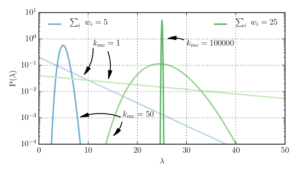
Figure 1: Examples of the distribution $P_{\mathrm{equal}}(\lambda;k_{mc}^{*},w)$ for the expectation value $\lambda$ using equal weights (eq. 19). The unique Prior is used, which means $k_{mc}^{*}=k_{mc}$. The distribution for $\sum w_{i}=5$ (blue) is shown for $1$ and $50$ MC events. The distribution for $\sum w_{i}=25$ (green) is shown for $1$, $50$ and $100000$ MC events.

As the number of sampling events $k_{mc}$ increases, one can see how the distribution approaches a delta peak centering around the sum of weights. To obtain the modified likelihood expression, we use eq. (10), which is solved analytically using eq. (LABEL:eq:exp_value_solution) in the appendix. The overall calculation reads

$$L_{\mathrm{\textbf{P},finite,eq.}} =\mathrm{E}\left[\frac{{e^{-\lambda}}{\lambda}^{k}}{k!}\right]_{{P_{\mathrm{equal}}(\lambda;k_{mc}^{*},w)}}$$

$$=\frac{(1/w)^{k_{mc}^{*}}\cdot\Gamma(k+k_{mc}^{*})}{\Gamma(k_{mc}^{*})\cdot k!\cdot(1+1/w)^{k+k_{mc}^{*}}}$$ (20)

$$\stackrel{{\scriptstyle[}}{{\alpha}}=0]{}{=}\frac{(\frac{k_{mc}}{\sum_{j}{w_{j}}})^{k_{mc}}\cdot(k+k_{mc}-1)!}{(k_{mc}-1)!\cdot k!\cdot(1+\frac{k_{mc}}{\sum_{j}{w_{j}}})^{k+k_{mc}}}$$ (21)

$$\stackrel{{\scriptstyle[}}{{\mathclap{}}}{\begin{subarray}{c}k_{mc}\rightarrow\infty\\ \sum_{j}w_{j}\rightarrow const.\end{subarray}}]{}{=}\frac{e^{-\sum_{j}w_{j}}\cdot(\sum_{j}w_{j})^{k}}{k!}$$

Since all weights are equal, $1/w=\frac{k_{mc}}{\sum_{j}w_{j}}$. The expression for all bins is a multiplication of this factor for each bin, just as for the usual situation of independently distributed Poisson data. Equation 20 can also be used as an approximate formula even if not all weights are equal, with $w$ being the mean weight of all weights in the bin. Equation 21, in this case shown for the unique Prior $\alpha=0$, is useful to derive the limiting standard Poisson behavior for $k_{mc}\rightarrow\infty$ and individual weights $w\rightarrow 0$. Other authors have considered eq. 20 previously in this context for the special case of Jeffreys Prior ($\alpha=0.5$) in Aggarwal2012.

2.2 General weights

The generalization to different weights per MC event follows directly from eq. (16) using arbitrary and possibly different weights for each factor in the convolution. Convolutions of general gamma distributions arise in many applications, e.g. in composite arrival time data Sim1992 or composite samples with weighted events DiSalvo98. The general solution can not be written down in a closed-form expression, but one can for example write it in terms of a generalized confluent hypergeometric function DiSalvo2008 or via a perturbative sum Moschopoulos1985. We choose the perturbation representation first (loosely following the notation in Moschopoulos1985), because it allows to easily calculate a result to a given desired precision. In the following, we treat the slightly more general case where we assume there are N distinct weights among the MC events which are enumerated with the index $j$ and come with multiplicities $k_{mc,j}$, the total number of MC events being $k_{mc}$. Then, the final expression for the convolution of $N$ general gamma-distributed Posteriors reads

$$P_{\mathrm{general}}(\lambda;\bm{k_{mc}},\bm{w})=C\cdot\sum_{l=0}^{\infty}{\delta_{l}\cdot\frac{\lambda^{\rho+l-1}\cdot e^{-\lambda/w_{N}}}{(\rho+l-1)!\cdot w_{N}^{\rho+l}}}$$ (22)

, where $w_{N}$ is the smallest weight in the bin, $\rho=\sum_{j}k_{{mc},j}^{*}=k_{{mc}}+\alpha$, $C=\prod_{j=1}^{N}(\frac{w_{N}}{w_{j}})^{k_{{mc},j}^{*}}$, $\gamma_{k}=\sum_{j=1}^{N}k_{mc,j}^{*}\frac{(1-w_{N}/w_{j})^{k}}{k}$ and $\delta_{k+1}=\frac{1}{k+1}\sum_{i=1}^{k+1}{i\cdot\gamma_{i}\cdot\delta_{k+1-i}}$ for positive integer k which is constructed iteratively with $\delta_{0}=1$ to the desired order. The term $k_{{mc},j}^{*}=k_{{mc},j}+k_{{mc},j}\cdot\alpha/k_{mc}$ corresponds to the definition in eq. (16), but generalized to $k_{{mc},j}$ weights per individual factor in the convolution. The overall behavior can be seen in figure 2, showing $P_{\mathrm{general}}(\lambda)$ for different examples of MC events which always sum to $10$.

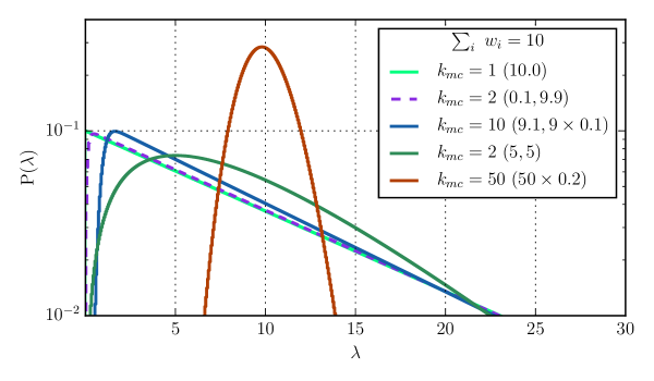
Figure 2: Examples of the distribution $P_{\mathrm{general}}(\lambda;\bm{k_{mc}^{*}},\bm{w})$ for the expectation value $\lambda$ using arbitrarily weighted Monte Carlo events (eq. 22). The unique Prior is used, which means $k_{mc,i}^{*}=k_{mc,i}$. The values in parenthesis indicate the weight distribution of these events, while the sum of all weights is always equal to $10$.

The distribution is usually dominated by events that are close to each other, as can be seen by the example with nine small weights and one large one (blue curve). The expression reduces to equation (19) when all weights are equal, since then $\delta_{0}=1$ and $\delta_{l}=0\ \forall\ l>0$. In the other extreme, as the spread between the weights gets larger, more and more terms in the perturbation series have to be taken into account in order to come close to the exact result. Since $\delta$, and thereby $P_{\mathrm{general}}(\lambda)$, is constructed iteratively, we can define a convenient stopping criterion for the iterative calculation. The desired relative precision $p$ can be reached by truncating the series when $C\cdot\sum_{i}\delta_{i}\approx p$, since $C\cdot\sum_{i=0}^{\infty}\delta_{i}=1$.

The next step is to form the corresponding generalization of the marginal likelihood for equal weights (eq. 20), i.e. integrating a Poisson factor mean $\lambda$ with $P_{\mathrm{general}}(\lambda)$. One possibility is to pull the integration inside the sum from eq. (22), and continue analogously to the equal-weights case. The result is an infinite series-representation of the marginal likelihood, and its calculation is shown in appendix LABEL:appendix:series_derivation. Here, however, we want to continue with the previously mentioned representation of $P_{\mathrm{general}}(\lambda)$ in terms of a generalized confluent hypergeometric function, since it is possible to derive an analytic closed-form expression along those lines. In this representation, $P_{\mathrm{general}}(\lambda)$ looks like DiSalvo2008

$$\begin{aligned} P_{\mathrm{general}}(\lambda)=\frac{\lambda^{k_{mc}^{*}-1}\cdot(1/w_{N})^{k_{mc}^{*}}e^{-\lambda\cdot(1/w_{N})}}{\Gamma(k_{mc}^{*})}\cdot\left(\prod_{j=1}^{N}\left(\frac{w_{N}}{w_{j}}\right)^{k_{mc,j}^{*}}\right)\\ \cdot\Phi_{2}^{*}(\bm{k_{mc,1\ldots N-1}^{*}};k_{mc}^{*};\lambda\cdot\bm{z^{*}})\end{aligned}$$ (23)

, where $N$ is the number of distinct weights, $w_{N}$ is the smallest weight, and $j$ enumerates like $j=1,\ldots,N-1$. The function $\Phi_{2}^{*}$ denotes the multidimensional generalization of the confluent Humbert series $\Phi_{2}$ with ${z^{*}}_{j}=1/w_{N}-1/w_{j}$. The corresponding Poisson marginal likelihood for one bin is again formed via the expectation value

$$\begin{aligned} L_{\mathrm{\textbf{P},finite,gen.}}&=\mathrm{E}\left[\frac{{e^{-\lambda}}{\lambda}^{k}}{k!}\right]_{P_{\mathrm{general}}(\lambda)}\end{aligned}$$

$$\begin{aligned} &=\int_{0}^{\infty}\frac{\lambda^{k_{mc}^{*}+k-1}\cdot(1/w_{N})^{k_{mc}^{*}}\cdot e^{-\lambda\cdot(1+1/w_{N})}}{\Gamma(k_{mc}^{*})\cdot k!}\\ &\cdot\left(\prod_{j=1}^{N}\left(\frac{w_{N}}{w_{j}}\right)^{k_{mc,j}^{*}}\right)\cdot\Phi_{2}^{*}(\bm{k_{mc,1\ldots N-1}^{*}};k_{mc}^{*};\lambda\cdot\bm{z^{*}})\ d\lambda\end{aligned}$$ (24)

$$\begin{aligned} &=\frac{\Gamma(k_{mc}^{*}+k)}{\Gamma(k_{mc}^{*})\cdot k!}\cdot\left(\frac{1}{w_{N}}\right)^{k_{mc}^{*}}\cdot\left(\frac{1}{1+1/w_{N}}\right)^{k_{mc}^{*}+k}\cdot\left(\prod_{j=1}^{N}\left(\frac{w_{N}}{w_{j}}\right)^{k_{mc,j}^{*}}\right)\\ &\cdot\int_{0}^{\infty}{\lambda^{*}}^{k_{mc}^{*}+k-1}e^{-\lambda^{*}}\cdot\Phi_{2}^{*}(\bm{k_{mc,1\ldots N-1}^{*}};k_{mc}^{*};\frac{\lambda^{*}}{1+1/w_{N}}\cdot\bm{z^{*}})\ d\lambda^{*}\end{aligned}$$ (25)

$$\begin{aligned} &=\frac{\Gamma(k_{mc}^{*}+k)}{\Gamma(k_{mc}^{*})\cdot k!}\cdot\left(\frac{1}{w_{N}}\right)^{k_{mc}^{*}}\cdot\left(\frac{1}{1+1/w_{N}}\right)^{k_{mc}^{*}+k}\\ &\cdot\left(\prod_{j=1}^{N}\left(\frac{w_{N}}{w_{j}}\right)^{k_{mc,j}^{*}}\right)\cdot F_{D}(k_{mc}^{*}+k;\bm{k_{mc,1\ldots N-1}^{*}};k_{mc}^{*};\bm{z^{**}})\end{aligned}$$ (26)

with $z^{**}_{j}=1-\frac{1+1/w_{j}}{1+1/w_{N}}$. A variable transform $\lambda^{*}=\lambda\cdot(1+1/w_{N})$ is used to form a Laplace-type integral (eq. 25) which is equivalent to the fourth Lauricella function $F_{D}$ via $F_{D}(a;\bm{b};c;\bm{z})=\int_{0}^{\infty}t^{a-1}e^{t}{\Phi_{2}^{*}}(\bm{b};c;t\cdot\bm{z})\ dt$ 1976Exton. The fourth Lauricella function is a certain extended form of the Gauss hypergeometric function, and appears for example in statistical problems Dickey1983 or even theoretical physics 1972Miller. For $F_{D}(a;\bm{b};c;\bm{z})$ with $\sum_{i}b_{i}<c$, as it is the case here, it is possible to evaluate $F_{D}$ via numerical integration of an integral representation over the simplex. However, this is not much more practical than the previously discussed series representation derived in appendix LABEL:appendix:series_derivation - both require long evaluation times for larger number of weights if the end result is supposed to be accurate, especially if the relative variation in the weights is large. However, for $a-c$ being a non-negative integer, which is the also the situation here, we can rewrite a generic $F_{D}$ via

$$F_{D}(a;\bm{b};c;\bm{z}) =R_{-a}(\bm{b_{+1}},1-\bm{z_{+1}})$$

$$=\left(\prod_{i}(1-z_{+1,i})^{-b_{+1,i}}\right)\cdot R_{a-c}\left(\bm{b}_{+1},(1-\bm{z}_{+1})^{-1}\right)$$

$$\begin{aligned} &=\left(\prod_{i}(1-z_{+1,1})^{-b_{+1,i}}\right)\\ &\cdot\left(\stackrel{{\scriptstyle[}}{{\sum}}_{i}k_{i}=a-c,\ k_{i}\geq 0]{}{\sum}\mathrm{\textbf{DM}}(\bm{k};\bm{b_{+1}})\prod_{i}(1-z_{+1,1})^{-k_{i}}\right)\end{aligned}$$ (27)

, where $F_{D}$ is expressed via Carlson’s Dirichlet average $R_{n}$ Carlson1963 in the first step. In the second step, we modify its first parameter Carlson1977 Neuman1994a from $-a$ to $a-c$, which picks up an extra factor. In the switch from $F_{D}$ to $R_{n}$, one always adds one element to $\bm{b}$ and $\bm{z}$, i.e. $\bm{z_{+1}}=[0,\bm{z}]$ and $\bm{b_{+1}}=[b_{0},\bm{b}]$ with $b_{0}=c-\sum_{i}b_{i}$, reflecting the homogeneity properties of $R_{n}$ Carlson1963. Looking back at eq. (26), we can identify $b_{0}$ with $k_{mc,N}^{*}$, i.e. the multiplicity and Prior factor of the smallest weight, which has been left out in $\bm{k_{mc,1\ldots N-1}^{*}}$ in the Lauricella function before, and subsequently $\bm{b_{+1}}=\bm{k_{mc}^{*}}$. In the last step we exploit that $R_{n}$ with non-negative integer $n$ is the probability generating function of a Dirichlet-multinomial distribution Dickey1983, which applies since $x=a-c=k_{mc}^{*}+k-k_{mc}^{*}=k$ is a non-negative integer. The Dirichlet-multinomial distribution is denoted by the factor DM. It can be derived as the expectation value of a multinomial distribution under a Dirichlet distribution Balakrishnan1997, and looks like

$$\mathrm{\textbf{DM}}(\bm{k};\bm{k_{mc}^{*}})=\frac{k!\cdot\Gamma(k_{mc}^{*})}{\Gamma(k+k_{mc}^{*})}\prod_{i}\frac{\Gamma(k_{i}+k_{mc,i}^{*})}{k_{i}!\cdot\Gamma(k_{mc,i}^{*})}$$ (28)

with $k=\sum_{i}k_{i}$ and $k_{mc}^{*}=\sum_{i}k_{mc,i}^{*}$. It will appear again later in the context of the generalization of the multinomial likelihood, where it might be easier to put it into context.

We will now simplify eq. (27) further. First we observe that parts of the combinatorial sum can be written in complex analysis form Zhou2011, namely

$$\stackrel{{\scriptstyle[}}{{\sum}}_{i}k_{i}=K,\ k_{i}\geq 0]{}{\sum}{\prod_{i}^{N}x_{i}^{k_{i}}}=\frac{1}{2\pi i}\oint\frac{t^{N+K-1}}{\prod_{i}(t-x_{i})}dt$$ (29)

where the contour integral is over the circle containing all $x_{i}$ on the inside. Next, we write $F_{D}$ for the case of the unique Prior and assume that all weights are different, i.e. $b_{+1,i}=k_{mc,i}^{*}=k_{mc,i}=1$. We write this as $\bm{b_{+1}}=\bm{1}=[1,\ldots,1]$), and for convenience use a modified argument $z_{i}\rightarrow 1-z_{i}^{-1}$, which results in

$$\begin{aligned} F_{D}(a;\bm{1}_{1\ldots N-1};c;1-\bm{z}^{-1})&=F_{D}(k+k_{mc};\bm{1}_{1\ldots N-1};k_{mc};1-\bm{z}^{-1})\end{aligned}$$

$$\begin{aligned} &=\left(\prod_{i}^{k_{mc}}(z_{+1,i})^{1}\right)\cdot\left(\stackrel{{\scriptstyle[}}{{|}}\bm{k}|=k,\ k_{i}\geq 0]{}{\sum}\mathrm{\textbf{DM}}(\bm{k};\bm{1})\prod_{i}^{k_{mc}}(z_{+1,i})^{k_{i}}\right)\end{aligned}$$

$$\begin{aligned} &=\mathrm{\textbf{DM}}(\bm{k};\bm{1})\cdot\left(\prod_{i}^{k_{mc}}z_{+1,i}\right)\cdot\frac{1}{2\pi i}\oint\frac{t^{k_{mc}+k-1}}{\prod_{i}^{k_{mc}}(t-z_{+1,i})}dt\end{aligned}$$ (30)

$$\begin{aligned} &=\frac{\Gamma(a-c+1)\cdot\Gamma(c)}{\Gamma(a)}\cdot\left(\prod_{i}^{c}z_{+1,i}\right)\cdot\frac{1}{2\pi i}\oint\frac{t^{a-1}}{\prod_{i}^{c}(t-z_{+1,i})}dt\end{aligned}$$

, where we first use eq. (27) to rewrite $F_{D}$ as a combinatorial sum. In the second step the Dirichlet-multinomial factor $\mathrm{\textbf{DM}}(\bm{k};\bm{1})$ is pulled out of the combinatorial sum in since it is constant for $b_{+1}=k_{mc,i}^{*}<2$, and we use eq. (29) to rewrite the whole expression via a contour integral. Just as a reminder, $a=k+k_{mc}$ and $c=k_{mc}$, as defined earlier. All weights $w_{i}$ are distinct by construction, so the $z_{i}$ are distinct as well since $z_{i}=\frac{1+1/w_{N}}{1+1/w_{i}}$ in the new nomenclature of $z_{i}$. We can now imagine two weights $w_{i}$, and thereby also the corresponding $z_{i}$, approach each other more and more, until they merge into a double pole in the contour integral (eq. 30) and the prefactor becomes $z_{+1,i}\rightarrow z_{+1,i}^{2}$. In general for $k_{mc,i}$ weights with equal weight, the pole becomes a pole with multiplicity $k_{mc,i}$ and the general expression for $F_{D}$ with $a>c$ and $c=\sum b_{+1,i}$ behaves as

$$F_{D}(a;\bm{b};c;1-\bm{z}^{-1})$$

$$=\frac{\Gamma(a-c+1)\cdot\Gamma(c)}{\Gamma(a)}\cdot\left(\prod_{i}^{N}{z_{+1,i}}^{b_{+1,i}}\right)\cdot\frac{1}{2\pi i}\oint\limits_{\rho=R\rightarrow\infty}\frac{t^{a-1}}{\prod_{i}^{N}(t-z_{+1,i})^{b_{+1,i}}}dt$$ (31)

$$=\frac{\Gamma(a-c+1)\cdot\Gamma(c)}{\Gamma(a)}\cdot(-1)^{b_{+1,i}}\cdot\frac{1}{2\pi i}\cdot\oint\limits_{\rho=\epsilon}\frac{1}{t^{a-c+1}\cdot\prod_{i}^{N}(t-1/{z_{+1,i}})^{b_{+1,i}}}dt$$ (32)

$$=\frac{\Gamma(a-c+1)\cdot\Gamma(c)}{\Gamma(a)}\cdot\left(\prod\limits_{i=1}^{N}{z_{+1,i}}^{b_{+1,i}}\right)\cdot D_{a-c}(\bm{b_{+1}},\bm{z_{+1}})$$ (33)

, where $N=\mathrm{len}(\bm{b})+1=\mathrm{len}(\bm{b_{+1}})$, $z_{+1,N}=1$, $b_{+1,N}=c-\sum_{i}b_{i}$ and the factor $D_{j}$ is iteratively defined via $D_{j}=\frac{1}{j}\sum\limits_{k=1}^{j}\left[\left(\sum\limits_{i=1}^{N}b_{+1,i}\cdot{z_{+1,i}}^{k}\right)D_{j-k}\right]$ with $D_{0}=1$. We first change the contour integral to a form which calculates the residue at infinity (eq. 32), which we subsequently write as a finite sum $D_{j}$ using the algorithm in Ma2014. Because we evaluate the integral with the residue at infinity, we can again allow for a Prior $\alpha\neq 0$, which generalizes $k_{mc}\rightarrow k_{mc}+\alpha=k_{mc}^{*}$. Thus, the above form of $F_{D}$ can be extended again to real $a$, $\bm{b}$ and $c$ (or to $k_{mc}^{*}$, $\bm{k_{mc}}^{*}$ and $k_{mc}^{*}+k$ in the other nomenclature for this concrete problem), retaining only the constraint that $a-c$ must be a non-negative integer.

To summarize, the reformulations of $F_{D}$ allow to write the single-bin Poisson likelihood incorporating uncertainty from finite Monte Carlo data (eq. 26) as

$$L_{\mathrm{\textbf{P},finite,gen.,1}}=\stackrel{{\scriptstyle[}}{{|}}\bm{k}|=k,\ k_{i}\geq 0]{}{\sum}\prod_{i}\frac{\Gamma(k_{i}+k_{mc,i}^{*})}{k_{i}!\cdot\Gamma(k_{mc,i}^{*})}\cdot\left(\frac{1}{w_{i}}\right)^{k_{mc,i}^{*}}\cdot\left(\frac{1}{1+1/w_{i}}\right)^{k_{i}+k_{mc,i}^{*}}$$ (34)

or

$$L_{\mathrm{\textbf{P},finite,gen.,2}}=\left(\prod_{i}\left(\frac{1}{1+w_{i}}\right)^{k_{mc,i}^{*}}\right)\cdot D_{k}(\bm{k_{mc}^{*}},\frac{1}{1+1/\bm{w}})$$ (35)

, by plugging in eq. (27) or eq. (33), respectively. The term $D_{k}$ is again iteratively defined as in eq. (33). The index $i$ goes over all distinct weights. It is quite remarkable, that in the latter representation all gamma factors cancel out, and one is left with one weight prefactor and an iterative finite sum $D_{k}$. For multiple bins, the full likelihood can be constructed as the product of the likelihood for each individual bins, similar to the standard Poisson likelihood for independently distributed data. The combinatorial sum (eq. 34) has an intuitive interpretation as marginalization of permutations, running over all possible combinations of counts $k_{i}$ distributed among the weights, and for each weight we have a factor corresponding to the result we earlier derived for a single weight (eq. 20). While this combinatorial expression very quickly becomes unmanageably large, the finite sum (eq. 35) has a substantial computational advantage and is more usable in practice. Due to the relation to Carlson’s Dirichlet average $R_{n}$ in eq. (27), the end result is also an efficient way to calculate several mathematical quantities including the probability generating function (PGF) of the Dirichlet-multionomial distribution, the general divided difference of a monomial function book:divdiv or moments of univariate B-Splines Carlson1991. More information can be found in appendix LABEL:appendix:pgf_and_others.

3 Finite-sample multinomial likelihood

Let us calculate the analogous finite-sample expression of the multinomial likelihood. The compound distribution in the multinomial case comes from the integration of bin probabilities $p_{i}$ instead of expectation values $\lambda$,

$$L_{\mathrm{\textbf{MN},finite}} =\mathrm{E}\left[{\textbf{MN}}(k_{1},\ldots,k_{N};p_{1},\ldots p_{N})\right]_{P(p_{1},\ldots,p_{N})}$$ (36)

$$=\stackrel{{\scriptstyle[}}{{\sum}}p_{i}=1]{}{\int_{p_{1}}\ldots\int_{p_{N}}}{\textbf{MN}}(k_{1},\ldots,k_{N};p_{1},\ldots p_{N})\cdot P(p_{1}\ldots,p_{N})\ dp_{1}\ldots dp_{N}$$ (37)

$$\begin{aligned} =\frac{k!}{k_{1}!\ldots k_{N}!}\stackrel{{\scriptstyle[}}{{\sum}}p_{i}\leq 1]{}{\int_{p_{1}}\ldots\int_{p_{N-1}}}p_{1}^{k_{1}}\cdot\ldots\cdot{p_{N-1}}^{k_{N-1}}\cdot\left(1-\sum_{i}^{N-1}{p_{i}}\right)^{k_{N}}\\ \cdot P(p_{1},\ldots,p_{N-1})\ dp_{1}\ldots dp_{N-1}\end{aligned}$$ (38)

with $N$ is equal to the number of bins. The integration happens over the $N-1$ simplex, and either has the constraint $p_{1}+\ldots p_{N}=1$ in eq. (37) or $p_{1}+\ldots+p_{N-1}\leq 1$ in eq. (38). The latter one is easier to work with in practice and we will usually do so in the rest of the paper.

3.1 Equal weights per bin

First, let us look at equal weights per bin. The analogue to the gamma distribution in the Poisson situation corresponds here to the scaled Dirichlet distribution Monti2011

$$\begin{aligned} P(p_{1},\ldots,p_{N-1})&=\frac{\Gamma(\alpha_{tot}^{*})}{\prod_{i}^{N}\Gamma(\alpha_{i}^{*})}\cdot\left(\prod_{i}^{N}{\beta_{i}^{*}}^{\alpha_{i}^{*}}\right)\cdot\frac{{p_{1}}^{\alpha_{1}^{*}-1}\ldots{p_{N-1}}^{\alpha_{N-1}^{*}-1}}{\left(\beta_{N}^{*}(1-\sum_{i}^{N-1}p_{i})+\sum_{i}^{N-1}\beta_{i}^{*}\cdot p_{i}\right)^{\alpha}}\\ &\cdot\left(1-\sum_{i}^{N-1}{p_{i}}\right)^{\alpha_{N}^{*}-1}\end{aligned}$$ (39)

, which can be derived as gamma random variables (one for each bin) which are each normalized according to their sum. To be consistent with the Poisson case, we again have $\alpha_{i}^{*}=k_{mc}^{*}=k_{mc,i}+\alpha_{i}$ and $\beta_{i}^{*}=1/w_{i}$ parameters that have a similar meaning as before, with the difference that $i$ now always stands for individual bins. Since the Prior should not depend on the bin, we set $\alpha_{i}=\alpha$. For the multinomial likelihood, there is no single-bin viewpoint, except the trivial one. For the parameter $\alpha_{tot}^{*}=\sum_{i}\alpha_{i}^{*}=k_{mc}+N\cdot\alpha$, we are in a similar consistency dilemma as before with the Poisson derivation - its value depends on the number of bins $N$, and would increase as more and more bins are taken into account. This means if we did not want this value to change with increased number of bins, we would have to go the other way around by defining $\alpha_{tot}^{*}=k_{mc}+\alpha$ and then redefine $\alpha_{i}^{*}=k_{mc,i}+\alpha/N$. Here, if more bins were used, it would be taken into account in the $\alpha_{i}^{*}$, but the overall $\alpha_{tot}^{*}$ would not change. Again, this dilemma can be solved by the unique Prior $\alpha=0$, where no such ambiguity exists, neither if more Monte Carlo events nor if more bins are being used. This issue will later become especially apparent for ratio-constructions (see section 4.2). For now, we use the first definition to be comparable to the Poisson case.

When the weights in all bins are equal, i.e. all $w_{i}=w$, $P$ reduces to the standard Dirichlet distribution and the compound likelihood (solution to the integral in eq. 38) becomes the already in eq. (28) introduced Dirichlet-multinomial distribution DM.

$$L_{\mathrm{\textbf{MN},finite,all\ equal}} =\mathrm{\textbf{DM}}(k_{1},\ldots,k_{N};k_{mc,1}^{*},\ldots,k_{mc,N}^{*})$$

The integration procedure using the general scaled Dirichlet density with different $\beta^{*}_{i}$ is more involved and calculated in detail in appendix LABEL:appendix:marginal_llh_multinomial. The final result looks like

$$\begin{aligned} \mathllap{L_{\mathrm{\textbf{MN},finite,eq.}}}&=\stackrel{{\scriptstyle[}}{{\sum}}p_{i}\leq 1]{}{\int_{p_{1}}\ldots\int_{p_{N-1}}}\mathrm{\textbf{MN}}(k_{1},\ldots,k_{N};p_{1},\ldots p_{N})\\ \cdot\frac{\Gamma(\alpha_{tot}^{*})}{\prod_{i}^{N}\Gamma(\alpha_{i}^{*})}&\cdot\left(\prod_{i}^{N}{\beta_{i}^{*}}^{\alpha_{i}^{*}}\right)\cdot\frac{{p_{1}}^{\alpha_{1}^{*}-1}\ldots{p_{N-1}}^{\alpha_{N-1}^{*}-1}}{\left(\beta_{N}^{*}(1-\sum_{i}^{N-1}p_{i})+\sum_{i}^{N-1}\beta_{i}^{*}\cdot p_{i}\right)^{\alpha_{tot}^{*}}}\\ &\cdot\left(1-\sum_{i}^{N-1}{p_{i}}\right)^{\alpha_{N}^{*}-1}\ dp_{1}\ldots dp_{N-1}\end{aligned}$$ (40)

$$\begin{aligned} &=\mathrm{\textbf{DM}}(\bm{k},\bm{k_{mc}^{*}})\cdot\left(\prod_{i}^{N}{\left(\frac{w_{N}}{w_{i}}\right)}^{k_{mc,i}}\right)\cdot F_{D}(a;\bm{b};c,\bm{z})\end{aligned}$$ (41)

, where $a=k_{mc}^{*}$, $b_{i}=k_{mc,i}^{*}+k_{i}\ (i=1\ldots N-1)$, $c=k_{mc}^{*}+k$, $z_{i}=1-w_{N}/w_{i}\ (i=1\ldots N-1)$. The resulting probability distribution consists of a Dirichlet-multinomial factor, a factor consisting of the weights, and again the fourth Lauricella function $F_{D}$. Compared to the Lauricella function appearing the Poisson case, however, this $F_{D}$ has the first and third argument switched, and the second vectorial argument is generally larger. When all weights are equal, the expression is again a standard Dirichlet-multinomial distribution, since $F_{D}(a,\bm{b},c,\bm{0})=1$. We can not simplify $F_{D}$ similarly to the Poisson case, since $c=k_{mc}^{*}+k>a=k_{mc}^{*}$. For this situation, other specific finite-sum representations have been found by Tan2005. However, they are a little more complicated in nature, and we do not write them out explicitly here.

For illustrative purposes, it is interesting to discuss that the Dirichlet-multinomial distribution $\mathrm{\textbf{DM}}(\bm{k},\bm{k_{mc}^{*}})$ for integer parameters, in this case this means for the unique Prior $k_{mc}^{*}=k_{mc}$, corresponds to a so-called standard Polya-Urn model Johnson1977. In this mental model, one draws differently colored balls from an urn, where the initial number of colored balls is fixed by a given color parameter. For each color drawn, one places the ball back, including an additional one of the same color. If one draws $K$ balls in this way, the $K$ balls are distributed according to the Dirichlet-multinomial distribution. This means, with the unique Prior, handling Monte Carlo simulations with equally weighted events in a multinomial evaluation with $N$ bins is exactly equivalent to a standard Polya-Urn modeling process with $N$ colors. In the multinomial Monte Carlo setup with equal weights per bin, the colors correspond to different bins, while the number of colored balls corresponds to the numbers of weighted Monte Carlo events $k_{mc,i}$ in a given bin $i$.

3.2 General weights

For general weights, it is not clear what the analogue for $P(\lambda)$ would be. However, we can draw inspiration from the combinatorial expression for the finite-sample Poisson likelihood (eq. 34). We can imagine that every weight individually corresponds to a single imaginary bin. For the numerator, we then have to find all combinations of $k_{i,j}$, the counts in the imaginary bins $j$, such that $\sum_{j}k_{i,j}=k_{i}$, where $k_{i}$ is the number of observed events in the real bin $i$. In the denominator, one relaxes this condition and sums over many more combinations with the only constraint that the total event count $k$ equals to the individual counts $k_{i,j}$ in the imaginary bins, independent of the real bin counts. The end result by construction has to be a probability distribution in $k_{i}$. The proposal distribution for the unique Prior that fulfills these criteria looks like

where zj=1-wN/wj(j=1…N-1) and wN is the smallest weight of all weights. The weight prefactor and Dirichlet-multinomial factor cancel out because every weight filled into the imaginary bins has single multiplicity kmc,i=1 by construction for the unique Prior, i.e. the Dirichlet-multinomial prefactor is just a constant. This formulation is also motivated by the ratio representation discussed in the next section. It has been checked to be a proper probability distribution for non-trivial binomial-like problems numerically, but it is just a motivated construction, not a solid mathematical derivation as a generalization of the case for equal weights per bin. In practice, it is also not very useful because of the huge combinatorial calculation. It would be interesting to know if a simpler representation exists.

Finally, all results from the multinomial likelihood automatically carry over to an approximated unbinned likelihood similarly to eq. (5) via a simple constant factor that depends on the binning. This can be useful in unbinned likelihood fits that combine analytic PDFs with MC-derived PDFs that are intrinsically binned and renormalized according to eq. (5). However, one can see that a difference to the standard multinomial formula is only seen if the weights in the different bins are not all the same. Otherwise the multinomial likelihood corresponds to the Dirichlet-Multinomial distribution, which in the categorical case, the case which matters for the unbinned formula discussed in eq. (5), is numerically equal to the standard multinomial formula for infinite statistics. Therefore, a difference can only be expected for MC-derived PDFs containing weighted simulation, not for data-derived PDFs where each event by definition has the same weight.

4 Further finite-sample constructions

With the generalized finite-sample expressions for the Poisson and multinomial case at hand, we can try to find relationships between the two. Let us recall that the multinomial likelihood is similar to a division of Poisson factors with a single global Poisson factor

$$L_{\mathrm{\textbf{MN}}} =\frac{\prod_{\mathrm{bins}\ i}L_{\mathrm{\mathbf{P}},i}}{L_{\mathrm{\mathbf{P},global}}}=\frac{\prod_{\mathrm{bins}\ i}\frac{e^{\lambda_{i}}\cdot\lambda^{k_{i}}}{{k_{i}}!}}{\frac{e^{\lambda}\cdot\lambda^{k}}{{k}!}}$$ (42)

$$=k!\cdot\prod_{\mathrm{bins}\ i}\frac{1}{{k_{i}}!}\left(\frac{\lambda_{i}}{\lambda}\right)^{k}$$ (43)

It turns out that the same relation does not hold anymore in the finite-sample limit. If we just replace the Poisson and Multinomial factors in eq. (42) with the finite-sample expressions from section 2 and section 3, we can check numerically that equality is slightly broken - with the exception of all weights in all bins being equal, i.e. when the Multinomial expression is the Dirichlet-multinomial distribution (see eq. 28). However, we can still try to perform such a construction and check what the outcome actually corresponds to. Interestingly, the results are slightly different probability distributions than the ”standard” finite-sample counterparts, and some of their properties are described in the following. For all expressions in this section, we use the unique Prior, i.e. α=0, as it seems to be the only sensible choice when expressions with different bin definitions are combined.

4.1 ”Product” construction for a likelihood of Poisson type

In this section, we take eq. (42) as inspiration and multiply a global finite-sample Poisson factor with a finite-sample Multinomial expression and then observe how the end result behaves. For equal weights per bin, we multiply eq. (41) with eq. (20) to obtain

$$L_{\mathrm{\mathbf{P},product,equal}} =L_{\mathrm{\mathbf{MN},equal}}\cdot L_{\mathrm{\mathbf{P},total,equal}}$$ (44)

and for general weights, we multiply eq. (LABEL:eq:finite_mnomial_general) with eq. (35) to obtain

$$L_{\mathrm{\mathbf{P},product,gen.}} =L_{\mathrm{\mathbf{MN},gen.}}\cdot L_{\mathrm{\mathbf{P},total,gen.}}$$ (45)

where for simplicity we do not write out the total expressions, as no insightful simplification is possible at this point. It turns out these ”product” expressions are multivariate probability distributions in k with a certain correlation structure imposed from the difference of the weights. A simple example with two bins is shown in figure 3.

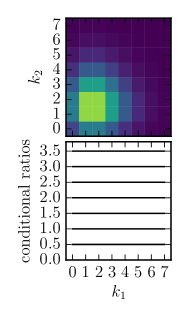
(a) Standard Poisson

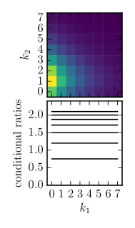
(b) Finite-sample Poisson

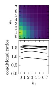
(c) Product construction

Figure 3: Different Poisson constructions for two bins compared by their PDFs of the counts $k_{1}$ and $k_{2}$. The first bin contains one weight with magnitude $2$, the second bin contains $4$ weights with magnitude $0.5$ each, so the sum of weights in both bins is equal. The upper plot shows the 2-d PDF (z-axis omitted, equal scale), the lower plot shows the ratio of conditional distributions $P(k_{1};k_{2}=i)/P(k_{1};k_{2}=i+1)$ for various $i$. The three Poisson-type formulas used for (a),(b),(c) are eq. (6), eq. (20) and eq. (44), respectively. The non-standard constructions use the unique Prior.

It depicts the difference between the standard Poisson likelihood (eq. 6), the finite-sample extension (eq. 20), and the product construction (eq. 44) for an artificial example with two bins: the first bin contains one weight with magnitude 2, the second bin four weights with magnitude 0.5 each, so the sum of weights is the same in each bin. The standard Poisson PDF in figure 3-(a) is symmetric, and does not know about the different weight distributions in the two bins. Also, the conditionals are flat, since the two Poisson factors for each bin are just multiplied with each other. The PDF for the finite-sample extension in figure 3-(b) has more confidence in the second bin, which contains more weights, and the distribution becomes asymmetric. The conditional distributions are still flat, since by construction the PDF is still a product of individual finite-sample Poisson factors which results in independently distributed random variables. The PDF for the product construction in figure 3-(c) is again asymmetric, but not independent anymore, as can be seen from the skewed ratios of conditional distributions. This dependence, or correlation, comes from the difference of the weights. If the weights were changed to be equal in all bins, the resulting distributions for (b) and (c) would be similar. Whether such a correlation is desired in practice remains to be seen, and would probably depend on the problem. The result implies that there are at least two principle ways to write a Poisson likelihood in the finite-sample limit - once as derived in section 2 by multiplying individual finite-sample Poisson factors for each bin, and once via a product construction that may contain multivariate correlation structure when the weights differ. When all weights in all bins are identical, which includes the limit of infinite statistics, both agree with each other.

4.2 ”Ratio” construction for a likelihood of multinomial type

For ”ratio” constructions, i.e. forming a multinomial-like expression from Poisson factors, we can derive some more rigorous and practical results. We start by writing the analogue of eq. (43) for finite Monte Carlo events assuming equal weights per bin. Using eq. (20) and eq. (26), the resulting expression looks like

$$L_{\mathrm{\textbf{MN},ratio,eq.}} =\frac{\prod_{i}L_{\mathrm{\mathbf{P},equal,i}}}{L_{\mathbf{P},general}}$$ (46)

$$\begin{aligned} &=\prod_{\mathrm{bins}\ i}\frac{(1/w_{i})^{k_{mc,i}}\cdot(k_{i}+k_{mc,i}-1)!}{(k_{mc,i}-1)!k_{i}!\cdot(1+1/w_{i})^{k_{i}+k_{mc,i}}}\Bigg{/}\\ &\Bigg{[}\frac{(k_{mc}+k)!}{(k_{mc}-1)!k!}\cdot\left(\frac{1}{w_{N}}\right)^{k_{mc}}\cdot\left(\frac{1}{1+1/w_{N}}\right)^{k_{mc}+k}\cdot\left(\prod_{j=1}^{N}\left(\frac{w_{N}}{w_{j}}\right)^{k_{mc,j}}\right)\\ &\cdot F_{D}(k_{mc}+k;\bm{b^{*}};k_{mc};\bm{z^{**}})\Bigg{]}\end{aligned}$$ (47)

$$=\mathrm{\textbf{DM}}(\bm{k};\bm{k_{mc}})\cdot\left(\prod_{i}\left(\frac{1+1/w_{N}}{1+1/w_{i}}\right)^{k_{mc,i}+k_{i}}\right)\cdot\frac{1}{F_{D}(k_{mc}+k;\bm{b^{*}};k_{mc};\bm{z^{**}})}$$ (48)

, consisting of a Dirichlet-multinomial factor, a factor depending on the weights, and the inverse of FD with specific arguments b∗i=kmc,i and z∗∗i=1-1+1/wi1+1/wN(i=1…N-1) where wN is the smallest weight in all bins. Since the Dirichlet-multinomial distribution DM is a proper probability density in k, i.e. the vector of observed counts in the individual bins, and eq. (48) is proportional to DM, we can write

$$L_{\mathrm{\textbf{MN},ratio,eq.}} =\mathrm{\textbf{DM}}(\bm{k};\bm{k_{mc}})\cdot\frac{\prod_{i}\left(\frac{1+1/w_{N}}{1+1/w_{i}}\right)^{k_{mc,i}+k_{i}}}{F_{D}(k_{mc}+k;\bm{b^{*}};k_{mc};\bm{z^{**}})}$$ (49)

$$=\mathrm{\textbf{DM}}(\bm{k};\bm{k_{mc}})\cdot\frac{C(\bm{k})}{\stackrel{{\scriptstyle[}}{{\sum}}_{i}k_{*,i}=k,\ k_{*,i}\geq 0]{}{\sum}\mathrm{\textbf{DM}}(\bm{k_{*}};\bm{k_{mc}})\cdot C(\bm{k_{*}})}$$ (50)

From this construction, we see that LMN,ratio,eq. is a probability distribution if C(k)=∏i(1+1/wN1+1/wi)kmc,i+ki and