Spitzer Observations of the North Ecliptic Pole

Abstract

We present a photometric catalog for Spitzer Space Telescope warm mission observations of the North Ecliptic Pole (NEP; centered at $\rm R.A.=18^{h}00^{m}00^{s}$, $\rm Decl.=66^{d}33^{m}38^{s}.552$). The observations are conducted with IRAC in 3.6 $\mu$m and 4.5 $\mu$m bands over an area of 7.04 deg² reaching 1$\sigma$ depths of 1.29 $\mu$Jy and 0.79 $\mu$Jy in the 3.6 $\mu$m and 4.5 $\mu$m bands respectively. The photometric catalog contains 380,858 sources with 3.6 $\mu$m and 4.5 $\mu$m band photometry over the full-depth NEP mosaic. Point source completeness simulations show that the catalog is 80% complete down to 19.7 AB. The accompanying catalog can be utilized in constraining the physical properties of extra-galactic objects, studying the AGN population, measuring the infrared colors of stellar objects, and studying the extra-galactic infrared background light.

1. Introduction

A statistical understanding of galaxy properties could be achieved by measuring the number counts of observed sources as a function of brightness in wide-area surveys (Jones et al. 1991; Pozzetti et al. 1998; Yasuda et al. 2001; Hatsukade et al. 2011; Valiante et al. 2016; Geach et al. 2017; Hemmati et al. 2017). This has been utilized successfully in the optical and near-infrared bands to study galaxy mass assembly and star-formation activity originating from stellar emission (e.g. Gardner et al. 1993; Fontana et al. 2014). Infrared observations of extragalactic sources has been made possible by the first generations of upper atmosphere probes and space missions (Harwit et al. 1966; Neugebauer & Leighton 1969; Neugebauer et al. 1984; Kessler et al. 1996), providing the first studies of non-stellar emission (Saunders et al. 1990; Genzel et al. 1998). In particular, all-sky observations by the Infrared Astronomical Satellite (IRAS; Neugebauer et al. 1984) and Wide-Field Infrared Survey Explorer (WISE; Wright et al. 2010) provided the first dust maps (Schlegel et al. 1998) and paved the way for detailed studies of populations of infrared-bright galaxies (Soifer et al. 1984; Genzel et al. 1998; Calzetti et al. 2000; Eisenhardt et al. 2012; Wu et al. 2012; Bridge et al. 2013).

The Spitzer Space Telescope (Werner et al. 2004) revolutionized studies of galaxy evolution by making crucial observations in the infrared revealing dust and stellar components in astronomical objects (Pérez-González et al. 2005; Draine & Li 2007; Magnelli et al. 2011). Spitzer deep and wide-field infrared observations over the past decade have produced a unique dataset (Dickinson et al. 2003; Lonsdale et al. 2003; Sanders et al. 2007; Ashby et al. 2009, 2013a, 2015) that has been used to study galaxy formation and evolution across a wide range of redshift and physical properties (Lacy et al. 2004; Le Floc’h et al. 2005; Brandl et al. 2006; Papovich et al. 2006).

In this work, we present catalogs of stellar and galactic objects identified from Spitzer Infrared Array Camera (IRAC; Fazio et al. 2004) observations of the North Ecliptic Pole (NEP). The NEP (centered at $\rm R.A.=18^{h}00^{m}00^{s}$, $\rm Decl.=66^{d}33^{m}38^{s}.552$) is the natural extragalactic deep field and has one of the deepest observations by several space observatories, including Planck and AKARI (Serjeant et al. 2012). It further has extensive observations from the X-ray to the millimeter (Kollgaard et al. 1994; Gioia et al. 2003; Lee et al. 2007; Jeon et al. 2010, 2014; Krumpe et al. 2015) with additional observations by WISE (Jarrett et al. 2011). The field was specifically chosen to match the observations by the Cosmic Infrared Background Experiment (CIBER; Bock et al. 2013; Zemcov et al. 2014) to study the extragalactic background light fluctuation (Cooray et al. 2004; Matsumoto et al. 2005; Cooray et al. 2012a; Zemcov et al. 2014; Matsuura et al. 2017). Figure 1 shows the sky coverage of the Spitzer NEP observations compared to the other infrared missions of the north ecliptic pole (Murakami et al. 2007; Matsuhara et al. 2006; Murata et al. 2013; Lee et al. 2009; Pilbratt et al. 2010; Bock et al. 2013). The Spitzer observations were designed to maximize overlap with those of AKARI (Murakami et al. 2007) in the Deep (Matsuhara et al. 2006; Murata et al. 2013) and Wide (Lee et al. 2009) fields and observations by Herschel (Pearson et al. 2017).

The Spitzer/IRAC dataset is complimentary to the already existing optical/near-infrared (Jeon et al. 2010, 2014) data and could be used in combination with those to constrain the stellar mass function of galaxies in the NEP. The Spitzer infrared observations in the NEP could additionally be utilized (in conjunction with the already existing X-ray observations; Krumpe et al. 2015) to identify AGNs (Stern et al. 2005). The NEP imaging data are particularly important for studies of diffuse light background fluctuations arising from individually un-detected sources directly probing early star-formation (Cooray et al. 2004, 2012a; Zemcov et al. 2014).

The paper is organized as follows. In Section 2 we present the imaging data and compilation for the Spitzer NEP field. Section 3 provides details on our source catalog and photometry estimation. We discuss our data analysis results in Section 4 and summarize our findings in Section 5. Throughout this paper we assume a standard cosmology with $H_{0}=70\,\text{kms}^{-1}\text{Mpc}^{-1}$, $\Omega_{m}=0.3$ and $\Omega_{\Lambda}=0.7$. All magnitudes are in the AB system where $\text{m}_{\rm AB}=23.9-2.5\times\text{log}(f_{\nu}/1\mu\text{Jy})$ (Oke & Gunn 1983).

2. Data

The North Eclipctic Pole, centered at $\rm R.A.=18^{h}00^{m}00^{s}$, $\rm Decl.=66^{d}33^{m}38^{s}.552$, was observed with Spitzer/IRAC in Cycle 10 (Program ID: 10147; PI: J. Bock). The observations were carried out over three epochs in both 3.6 $\mu$m and 4.5 $\mu$m bands (Table 1). The first two epochs were separated by $\sim 10$ weeks and epoch three was observed $\sim 8$ weeks after epoch two. The observations in different epochs enables study of the zodiacal light contamination, which changes throughout the year, for background fluctuations (Cooray et al. 2012a).

Three epochs were considered sufficient for mapping the Spitzer NEP, based on previous observations of SDWFS (Ashby et al. 2009), as this provided reliable power spectra measurements for studying the intra-halo light (IHL) and extragalactic background light (EBL) (Cooray et al. 2012b; Zemcov et al. 2014) combined with existing CIBER and AKARI data in the field. The mapping strategy involved observations that were offset by one-third of the IRAC field of view between successive passes through each group (where we split the field into sixteen groups) and were dithered on small scales to maximize the inter-pixel correlation to facilitate self-calibrations. Furthermore, to ensure that asteroids are reliably identified, each group is observed in three passes of 30 sec each. The time required to obtain a single 30 sec pass on a group ensures gaps of at least 2 hours between observations of each sky position. For typical asteroid motions of 25 arcsec hour^-1, asteroids will move 1 arcmin between maps. Since this is much smaller than a typical map width, three map observations will reliably track asteroid motions. We further note here that there are very unlikely to be any main belt asteroids (with a 25 arcsec hour^-1 motion) in the Ecliptic Cap, with most being near the Ecliptic Plane. Some near-earth asteroids may be present, but these typically have much faster motions ($\sim$ several arcmin/hr) and easily identifiable.

Basic Calibrated Data (BCD) and associated files were directly downloaded from the Spitzer Science Center after acquisition. This corresponds to 3936 tiles in each epoch in each of the bands (except epoch 2 which observed 3854 tiles in 3.6 $\mu$m; see Table 1) with 23.6 sec and 26.8 sec exposures per tile at 3.6 $\mu$m and 4.5 $\mu$m, respectively. This resulted in a continuous Spitzer map of the NEP field covering an area of 7.04 deg² corresponding to a total integration time of $\rm\sim 165\,h$. Figure 2 shows the NEP area coverage and depth compared to other Spitzer surveys.

Table 1Observations Summary^†.

Epoch	Observation Dates	No. BCDs 3.6 $\mu$m/4.5 $\mu$m	Exposure Timea 3.6 $\mu$m/4.5 $\mu$m	Exposure time per pixelb 3.6 $\mu$m/4.5 $\mu$m
			(hours)	(seconds)
1	May 06-09, 2014	3936/3936	25.8/29.3	106/120
2	Jul 18-24, 2014	3854/3936	25.3/29.3	104/119
3	Sep 08-14, 2014	3936/3936	25.8/29.3	107/121
Total	$-$	11808/11726	76.9/87.9	282/331c

^†: Cycle 10 program Spitzer/IRAC observations (PID: 10147). ^a: Total exposure time of each mosaic. ^b: The average exposure time per pixel in each mosaic. ^c: Measured as the average value from the combined three epoch mosaic exposure maps.

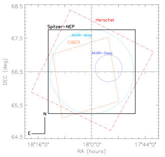
Figure 1.— The areal coverage of the Spitzer North Ecliptic Pole (centered at $\rm R.A.=18^{h}00^{m}00^{s}$, $\rm Decl.=66^{d}33^{m}38^{s}.552$) compared to that of AKARI (Murakami et al. 2007) in the Deep (Matsuhara et al. 2006; Murata et al. 2013) and Wide (Lee et al. 2009) fields, CIBER (Bock et al. 2013; Zemcov et al. 2014) and Herschel (Pearson et al. 2017). The Spitzer observations were chosen to maximize the sky coverage by all these surveys providing a complete census of the infrared SEDs of galaxies.

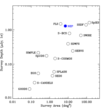
Figure 2.— Observations depth and sky coverage of the NEP (at the 3.6 $\mu$m) compared to other Spitzer surveys. These include the Great Observatories Origins Deep Survey (GOODS; Dickinson et al. 2003; Giavalisco et al. 2004), Spitzer-Cosmic Assembly Near-infrared Deep Extragalactic Legacy Survey (S-CANDELS; Ashby et al. 2015), Extended Groth Strip (EGS; Davis et al. 2007), Spitzer Extended Deep Survey (SEDS; Ashby et al. 2013a), Spitzer Large Area Survey with Hyper-Suprime-Cam (SPLASH; Capak et al. 2013), S-COSMOS (Sanders et al. 2007), Spitzer Public Legacy Survey of UKIDSS Ultra-deep Survey (SpUDS; Caputi et al. 2011), Spitzer IRAC/MUSYC Public Legacy in E-CDFS (SIMPLE; Damen et al. 2011), Spitzer Deep Wide-Field Survey (SDWFS; Ashby et al. 2009), Spitzer Wide-area Infrared Extragalactic Survey (SWIRE; Lonsdale et al. 2003), Spitzer Blanco Cluster Survey (S-BCS), First Look Survey (FLS; Lacy et al. 2005), Spitzer Extragalactic Representative Volume Survey (SERVS; Mauduit et al. 2012), Spitzer-IRAC Equatorial Survey (SpIES) and Spitzer South Pole Telescope Deep Field (SSDF; Ashby et al. 2013b). The NEP covers an area of 7.04 deg² reaching a 1$\sigma$ depth of 1.29 $\mu$Jy (measured over an aperture of $4^{\prime\prime}$).

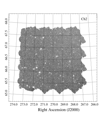
Figure 3.— The combined three epoch Spitzer maps of the North Ecliptic Pole (NEP) in the 3.6 $\mu$m (left) and the 4.5 $\mu$m band (right) as part of Cycle 10 observations with total exposure time of $\rm\sim 165\,h$ during the warm mission over an area $\rm\sim 7.04\,deg^{2}$.

We used mopex version 18.5.0 (Makovoz et al. 2006) on the corrected-Basic Calibrated Data (cBCDs) released by the Spitzer Science Center to construct the mosaics. We generated combined mosaics for each epoch and a combined mosaic of all three epochs with mopex for the 3.6 $\mu$m and 4.5 $\mu$m observations. Figure 3 shows the combined three epoch mosaics in the 3.6 $\mu$m and 4.5 $\mu$m bands. In Summary mopex takes the data frames along with the associated uncertainty frames and constructs a Fiducial Image Frame (FIF) from the boundaries of the data frame onto which input observations will be projected. It then runs a background matching routine on overlapping frames and performs an image interpolation which maps the individual frames onto the generated FIF after which a co-added mosaic image is generated. During the process mopex also performs an outlier rejection routine to identify outlier pixels (such as cosmic rays) and generates a bad pixel mask which is used in the construction of the mosaic. Each generated science map is also accompanied by the corresponding uncertainty and exposure maps calculated by mopex. We refer the reader to the mopex manual for further details. Figure 4 shows the mopex generated coverage map of the NEP for the full depth mosaics in the 3.6 $\mu$m and 4.5 $\mu$m bands. We see that the NEP observations have very uniform depth across the field in both bands. Figure 5 shows the area coverage of the 3.6 $\mu$m map given a minimum exposure time for a single epoch and the full depth mosaics. We see that more than 89% of the field (with area $\rm\sim 6.26\,deg^{2}$) is covered with an exposure time of at least 100 sec in the full depth mosaic whereas only 45% (with area $\rm\sim 3.17\,deg^{2}$) is covered to similar depths in a single epoch. The individual 3.6 $\mu$m epochs have 1$\sigma$ depths of 2.11 $\mu$Jy, 2.13 $\mu$Jy and 2.22 $\mu$Jy respectively in the three epochs and a depth of 1.29 $\mu$Jy over the combined full depth mosaic. The combined full depth mosaic in the 4.5 $\mu$m band has a 1$\sigma$ depth of 0.79 $\mu$Jy (measured over an aperture of 4^′′ with aperture corrections applied; see Section 3.2). Table 1 summarizes the Spitzer NEP observations.

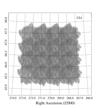
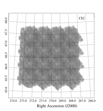
Figure 4.— The combined three epoch Spitzer 3.6 $\mu$m (left) and 4.5 $\mu$m (right) coverage maps demonstrating the depth uniformity across the field. This consists of total of 11808 and 11726 individual tiles in 3.6 $\mu$m and 4.5 $\mu$m bands respectively over three epochs.

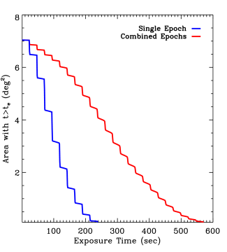
Figure 5.— Area coverage of the Spitzer 3.6 $\mu$m NEP map as a function of total exposure time for the combined three epochs (in red) and a single epoch (in blue). More than 89% of the field is covered with exposure time of at least 100 sec in the combined mosaic where that number is 45% for the single epoch observations. Table 1 summarizes the exposure time in each epoch.

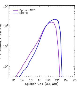
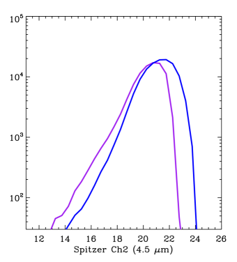
Figure 6.— Left: Normalized 3.6 $\mu$m number counts of sources in the Spitzer NEP catalog (magenta) compared to the counts in the SDWFS (blue). The SDWFS is a deeper survey (see Figure 2) and this is reflected in the counts at the faint end. On the other had the Spitzer NEP shows a larger number of sources at the bright end. Right: Number counts of sources in the Spitzer NEP 4.5 $\mu$m band compared to the SDWFS (Ashby et al. 2009).

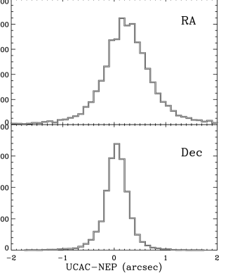
Figure 7.— Distribution of the difference in right ascension (top) and declination (bottom) of the Spitzer NEP catalog to that of USNO CCD Astrograph Catalog (UCAC4; Zacharias et al. 2013). The NEP shows an offset of 0^′′.25 in the right ascension (smaller than the Spitzer mosaic pixel) compared to the UCAC catalog whereas the Declination distribution is consistent with a zero offset. The distributions have standard deviations of 0^′′.51 and 0^′′.24 in the right ascension and declination respectively that are smaller than that of the IRAC PSF FWHM.

3. Source Catalogs

3.1. Source Identification and Photometry

We used SExtractor (Bertin & Arnouts 1996) for source identification and photometry. SExtractor is run in dual mode on the combined three epoch mosaics on the 3.6 $\mu$m and 4.5 $\mu$m individually as the detection bands with photometry extracted in both. The two catalogs are then merged to form the final NEP catalog. With this approach, we make sure to include 3.6 $\mu$m faint sources that are detected in the 4.5 $\mu$m and would have been missed by the former selection alone. The mopex generated mosaics are in units of $\rm[MJy\,Sr^{-1}]$, which we convert to $\rm[\mu Jy\,pixel^{-1}]$ using the map pixel scale of $1^{\prime\prime}.2$ before measuring the photometry. We used a minimum detection area of 3 pixels with a detection threshold of 2$\sigma$ for source identification. This is chosen to maximize the recovered sources while minimizing spurious source identification. We identify 380,858 sources over the 7.04 deg² area of the Spitzer NEP map with our detection criteria. We measure source photometry in AB magnitudes given the pixel flux units in micro-Jansky and report this in a Kron radius (the mag_auto), which is photometry over an ellipse with size and orientation determined from the second moment of light distribution above the isophotal threshold, and also over two apertures (with $4^{\prime\prime}$ and $6^{\prime\prime}$ diameter). We further report the SExtractor measured stellarity parameter for each object which we use later (see Section 4.4) to validate the color of stars in the field. Figure 6 shows the area-normalized distribution of the source photometry in the full NEP of the combined three epochs.

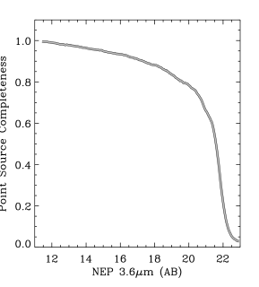
Figure 8.— Simulated point source completeness fraction at 3.6 $\mu$m as a function of source magnitude. Point sources are generated from the IRAC 3.6 $\mu$m PSF and are randomly distributed over the NEP mosaic. The recovered fraction using the original SExtractor parameters, used to generate the photometric catalog, provides the completeness.

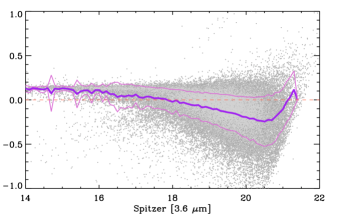
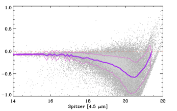
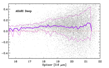
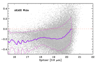
Figure 9.— Top: The photometric comparison of the Spitzer NEP to that of WISE (Wright et al. 2010) for the NEP 3.6 $\mu$m (left) and 4.5 $\mu$m bands. We use the AllWISE catalog (Cutri 2013) photometry measurements in the W1 (at 3.4 $\mu$m) and W2 (at 4.6 $\mu$m) bands to compare with NEP catalog respectively. The NEP photometry is consistent with WISE showing small scatter with magnitude offsets associated with variations in the filter response function shapes between Spitzer and WISE. Bottom: Photometric comparison of the IRAC 3.6 $\mu$m in the NEP to that of the AKARI deep (left) (Murata et al. 2013) and AKARI wide (right) (Kim et al. 2012). The AKARI photometry is taken from the average of the fluxes in the two AKARI infrared bands of N3 and N4 (at 3.2 $\mu$m and 4.1 $\mu$m respectively).

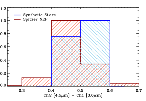
Figure 10.— The observed $\rm(4.5\,\mu m-3.6\,\mu m)$ color distributions of stars in the Spitzer NEP catalog (in red) compared to the color of template stellar models from BaSeL library (Lejeune et al. 1997, 1998; Westera et al. 2002). The NEP stars are selected using the SExtractor stellarity parameter assuming class_star $>0.9$. The stellar model colors are computed using the Spitzer filter response functions. The observed IRAC color of stars is consistent with predictions from the BaSeL library, with mean colors of 0.54 and 0.51 respectively. The scatter in the observed IRAC color is associated with the photometric uncertainties in the NEP catalog.

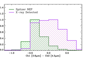
Figure 11.— The observed IRAC $\rm(3.6\,\mu m-4.5\,\mu m)$ color distribution of all Spitzer NEP sources (in green) compared to the X-ray detected objects (Krumpe et al. 2015) (in magenta). The distribution of IRAC color of X-ray sources is consistent with the AGN colors reported in Stern et al. 2005.

3.2. Aperture Corrections

We perform aperture photometry over two circular apertures at fixed $4^{\prime\prime}$ and $6^{\prime\prime}$ diameters in addition to the SExtractor measured mag_auto discussed above. The fixed apertures often under-predict the flux of objects. We corrected the aperture photometry measurements in the 3.6 $\mu$m and 4.5 $\mu$m bands for the effect of fixed apertures (at $4^{\prime\prime}$ and $6^{\prime\prime}$) used in their measurements. For this we used the curve of growth of five isolated stars in the field using ever growing circular apertures (with $4^{\prime\prime}-10^{\prime\prime}$ diameter) to measure the source flux. The aperture correction is measured as the mean of the correction from the curve of growth of the selected stars. Table 2 summarizes the aperture corrections (in AB magnitudes) for both observed IRAC bands. These agree with the reported numbers by Ashby et al. (2009) for the SDWFS and also corrections reported by the IRAC Instrument Handbook.

Table 2Aperture Corrections^†.

Aperture Diameter	3.6 $\mu$m band	4.5 $\mu$m band
$3^{\prime\prime}$	-0.65	-0.65
$4^{\prime\prime}$	-0.36	-0.46
$5^{\prime\prime}$	-0.22	-0.28
$6^{\prime\prime}$	-0.15	-0.19

^†: Measured from point-sources curve of growth.

3.3. Astrometry

We validate the astrometry of the Spitzer NEP catalog generated by SExtractor against the publicly available USNO CCD Astrograph Catalog (UCAC; Zacharias et al. 2013) fourth version. We use a 2^′′ radius to cross-match the NEP catalog with that of UCAC. We further limit the astrometry analysis to sources with a minimum signal-to-noise ratio of 20 in the NEP 3.6 $\mu$m band. This generates a catalog of 8729 sources over the full NEP area. Figure 7 shows the distribution of the difference in right ascension and declination between the NEP catalog and the UCAC. The distribution of the difference in declination is consistent with being centered on zero with a deviation of 0^′′.04, whereas the right ascension difference shows a mean offset of 0^′′.25. These distributions have standard deviations of 0^′′.51 and 0^′′.24 in the right ascension and declination respectively, smaller than the IRAC spatial resolution measured from the PSF FWHM ($\sim 1^{\prime\prime}.78$). We note here that the offset is also smaller than the pixel scale of our Spitzer/IRAC mosaics at 1^′′.2 and that we did not apply this to the final photometric catalog. The final photometric catalog will be available through the IRSA website and as a machine readable table with this publication. Table 3 in the appendix summarizes the entries in the published catalog.

4. Analysis

4.1. Number Counts

The Spitzer NEP 3.6 $\mu$m selected catalog has 380,858 sources over an area of 7.04 deg². Figure 6 shows the NEP area-normalized source number counts along with the source counts from the Spitzer Deep Wide-Field Survey (SDWFS; Ashby et al. 2009) in the 3.6 $\mu$m and 4.5 $\mu$m. The variations in the number count distributions are associated with the larger number of stars and shallower depths (see Figure 2) at the bright and faint end respectively in the NEP compared to that of SDWFS. Table 3 summarizes the source counts of the photometric catalog in designated magnitude bins along with the associated Poisson uncertainties.

Table 3Spitzer/IRAC 3.6 $\mu$m number counts in the NEP catalog.

Spitzer/IRAC 3.6 $\rm\mu m^{\dagger}$	N ($\text{deg}^{-2}\text{mag}^{-1}$)	Poisson Uncertainty
14.25	121	6
14.75	170	7
15.25	259	9
15.75	404	11
16.25	586	13
16.75	845	15
17.25	1270	19
17.75	1927	23
18.25	3222	30
18.75	5522	40
19.25	8605	49
19.75	11811	58
20.25	14422	64
20.75	15205	66

^†: Bin center magnitude.

4.2. Completeness Estimates

To get an estimate of the NEP survey catalog depth we performed a point-source completeness estimate on the combined three epoch full depth in the 3.6 $\mu$m band. For this we generated a large number of point sources of varying brightness (with 1000 sources in each 0.05 bins of magnitude), given the IRAC PSF FWHM (at $1^{\prime\prime}.78$). We then randomly distributed these sources across the 3.6 $\mu$m mosaic while avoiding the mosaic edges and existing objects in the field using the segmentation map generated by SExtractor for the main photometric catalog. We used the original SExtractor detection criteria to identify sources in the new co-added map of real and simulated objects. We cross-matched the generated catalog with the known simulated positions of the injected sources which yields a recovery fraction of the point sources. Figure 8 shows the recovered fraction of the simulated point sources as a function of the source brightness. The catalog has a point source completeness estimate 80% for objects with 19.71 (AB mag) in the 3.6 $\mu$m and drops rapidly for faint sources.

4.3. Photometric Validation Check

To check the robustness of the Spitzer measured photometry, we compared our IRAC measured photometry with that of the Wide-Field Infrared Survey Explorer (WISE; Wright et al. 2010). For this, we used the AllWISE catalog (Cutri 2013) to extract the WISE photometry in the W1 and W2 bands (at 3.4 $\mu$m and 4.6 $\mu$m respectively). We used the conversion factors provided in Table 1 of Jarrett et al. (2011) to convert the WISE measured Vega magnitudes in the W1 and W2 bands to AB magnitudes for comparison. Figure 9 shows the comparison of Spitzer measured magnitudes in the 3.6 $\mu$m and 4.5 $\mu$m bands to that of WISE W1 and W2 observations in the NEP. The Spitzer measured photometry in consistent with WISE with a small scatter at bright magnitudes ($\rm\sigma(m)=0.03$ for 3.6 $\mu$m and $\rm\sigma(m)=0.01$ for 4.5 $\mu$m; computed at $\rm m_{AB}=15$) increasing to $\rm\sigma(m)=0.23$ for 3.6 $\mu$m and $\rm\sigma(m)=0.32$ for 4.5 $\mu$m for fainter objects (measured at $\rm m_{AB}=20$). The Spitzer photometry is offset from WISE by $\rm\Delta m=0.13$ and $\rm\Delta m=0.07$ in the 3.6 $\mu$m and 4.5 $\mu$m respectively (measured from the bright end). This is associated with differences in the filter response functions and effective wavelengths probed creating a zero-point offset. We do not apply these offsets to the our Spitzer NEP photometric catalog.

We further compared our IRAC photometry in the Spitzer NEP with infrared observations by the AKARI in the north ecliptic pole. For this we used the catalog of sources in the AKARI deep and wide surveys of the north ecliptic pole (Murata et al. 2013; Kim et al. 2012), covering an area of 0.5 deg² and 5.4 deg² respectively. Figure 9 shows the comparison of the 3.6 $\mu$m photometry to that of AKARI. For the comparison, we take the average of the fluxes in the AKARI N3 and N4 filters (at 3.2 $\mu$m and 4.1 $\mu$m respectively; Murata et al. 2013). We see from the figure that, on average, the measured IRAC 3.6 $\mu$m photometry agrees well with that of AKARI, specially at the bright end and for the AKARI deep observations. The main source of the deviation is associated with the differences in the Spitzer filter response function and the average filter functions associated with the combined AKARI N3 and N4 observations.

4.4. IRAC Color

We further check the validity of the Spitzer measured photometry by comparing the color distribution of stars in the NEP survey to the expected infrared color derived from stellar model templates. For this we used the BaSeL stellar library (Lejeune et al. 1997, 1998; Westera et al. 2002) and computed the expected color of model templates by integrating over the stellar SEDs given the Spitzer/IRAC filter response functions at 3.6 $\mu$m and 4.5 $\mu$m. Figure 10 shows the expected $\rm Ch2\,[4.5\,\mu m]-Ch1\,[3.6]\,\mu m$ color of stellar models compared to measured colors of stars in the NEP catalog. We identified stellar sources in the NEP catalog using the stellarity parameter, class_star, from SExtractor requiring class_star $>0.99$. This gives 2107 stellar objects for the NEP catalog. The IRAC color distribution of stars in the NEP catalog is consistent with stellar model predictions with mean $\rm(4.5\,\mu m-3.6\,\mu m)$ values of 0.47 and 0.50 for the observed color of stars from NEP catalog and measured color from template stellar models respectively. The scatter in the NEP IRAC colors is associated with the photometric uncertainties in individual flux measurements.

4.5. X-ray Sources

The Spitzer/IRAC colors have been used to identify populations of active galaxies (Stern et al. 2005; Donley et al. 2012) where the continuum flux is expected to be dominated by a power law for AGN dominated sources. These selections use the IRAC observations in four filters to isolate the AGN selection area on the color-color diagram. Due to lack of longer wavelength Spitzer observations (at 5.8 $\mu$m and 8.0 $\mu$m), we instead look at the $\rm(3.6\,\mu m-4.5\,\mu m)$ color distribution of sources in the NEP catalog. Figure 11 shows the IRAC color distribution of all the NEP sources compared to the X-ray detected sources in the field. We used the Chandra AKARI NEP X-ray point source catalog (Krumpe et al. 2015) and used a 2^′′ matching radius to extract the IRAC colors. This gives 354 matched sources with the X-ray catalog. We see that the X-ray sources have a redder $\rm(3.6\,\mu m-4.5\,\mu m)$ color distribution, on average, compared to the full sample as expected for AGN samples (Stern et al. 2005).

5. Summary

Here we presented a Spitzer/IRAC combined mosaics and a 3.6 $\mu$m and 4.5 $\mu$m detected catalog of extra-galactic sources in the North Ecliptic Pole (NEP; centered at $\rm R.A.=18^{h}00^{m}00^{s}$, $\rm Decl.=66^{d}33^{m}38^{s}.552$). The catalog contains IRAC photometry for 380,858 sources in the 3.6 $\mu$m and 4.5 $\mu$m bands. Here are the main findings:

• The combined three epoch full-depth mosaic covers an area of 7.04 deg² reaching 1$\sigma$ depths of 1.29 $\mu$Jy and 0.79 $\mu$Jy, over an aperture of 4^′′ in diameter, in the 3.6 $\mu$m and 4.5 $\mu$m bands respectively.

• The mosaics have uniform exposure across the field with more than 89% of the field covered by an exposure time of at least 100 sec.

• The photometric catalog has astrometry offset and uncertainties consistent with the Spitzer PSF FWHM and pixel size.

• The Spitzer/IRAC measured photometry in the NEP is consistent with earlier measurements by WISE and AKARI at similar wavelengths with current IRAC observations being deeper than both.

• The colors of stellar objects in the NEP agrees with colors of stellar template models and also agrees with expected colors of X-ray detected sources, further validating the measured photometry.

• The generated IRAC point-source catalogs will be available through the NASA/IPAC Infrared Science Archive.

Appendix: Photometric Catalog Entries

The entries in the Spitzer/IRAC photometric catalog for the North Ecliptic Pole.

# 1 ID
# 2 R.A.
# 3 Decl.
# 4 IRAC 3.6 $\mu$m Auto Magnitude (AB)
# 5 IRAC 3.6 $\mu$m Auto Magnitude Error (AB)
# 6 IRAC 4.5 $\mu$m Auto Magnitude (AB)
# 7 IRAC 4.5 $\mu$m Auto Magnitude Error (AB)
# 8 IRAC 3.6 $\mu$m Aperture1 Magnitude (AB)
# 9 IRAC 3.6 $\mu$m Aperture1 Magnitude Error (AB)
# 10 IRAC 4.5 $\mu$m Aperture1 Magnitude (AB)
# 11 IRAC 4.5 $\mu$m Aperture1 Magnitude Error (AB)
# 12 IRAC 3.6 $\mu$m Aperture2 Magnitude (AB)
# 13 IRAC 3.6 $\mu$m Aperture2 Magnitude Error (AB)
# 14 IRAC 4.5 $\mu$m Aperture2 Magnitude (AB)
# 15 IRAC 4.5 $\mu$m Aperture2 Magnitude Error (AB)
# 16 CLASS_STAR

Notes:
Col. (1): Sequential number.
Col. (2) & (3): Target coordinates (in degrees).
Col. (4) - (7): 3.6 $\mu$m and 4.5 $\mu$m photometry over Kron radius (AB mag)
Col. (8) - (11): 3.6 $\mu$m and 4.5 $\mu$m aperture photometry with a $4^{\prime\prime}$ diameter aperture (AB mag)
Col. (12) - (15): 3.6 $\mu$m and 4.5 $\mu$m aperture photometry with a $6^{\prime\prime}$ diameter aperture (AB mag)
Col. (16): SExtractor stellarity parameter.

References

- Ashby et al. (2009) Ashby, M. L. N., Stern, D., Brodwin, M., et al. 2009, ApJ, 701, 428
- Ashby et al. (2013a) Ashby, M. L. N., Willner, S. P., Fazio, G. G., et al. 2013a, ApJ, 769, 80
- Ashby et al. (2013b) Ashby, M. L. N., Stanford, S. A., Brodwin, M., et al. 2013b, ApJS, 209, 22
- Ashby et al. (2015) Ashby, M. L. N., Willner, S. P., Fazio, G. G., et al. 2015, ApJS, 218, 33
- Bertin & Arnouts (1996) Bertin, E., & Arnouts, S. 1996, A&AS, 117, 393
- Bock et al. (2013) Bock, J., Sullivan, I., Arai, T., et al. 2013, ApJS, 207, 32
- Brandl et al. (2006) Brandl, B. R., Bernard-Salas, J., Spoon, H. W. W., et al. 2006, ApJ, 653, 1129
- Bridge et al. (2013) Bridge, C. R., Blain, A., Borys, C. J. K., et al. 2013, ApJ, 769, 91
- Calzetti et al. (2000) Calzetti, D., Armus, L., Bohlin, R. C., et al. 2000, ApJ, 533, 682
- Capak et al. (2013) Capak, P., Aussel, H., Bundy, K., et al. 2013, SPLASH: Spitzer Large Area Survey with Hyper-Suprime-Cam, Spitzer Proposal
- Caputi et al. (2011) Caputi, K. I., Cirasuolo, M., Dunlop, J. S., et al. 2011, MNRAS, 413, 162
- Cooray et al. (2004) Cooray, A., Bock, J. J., Keatin, B., Lange, A. E., & Matsumoto, T. 2004, ApJ, 606, 611
- Cooray et al. (2012a) Cooray, A., Gong, Y., Smidt, J., & Santos, M. G. 2012a, ApJ, 756, 92
- Cooray et al. (2012b) Cooray, A., Smidt, J., de Bernardis, F., et al. 2012b, Nature, 490, 514
- Cutri (2013) Cutri, R. M. 2013, VizieR Online Data Catalog, 2328
- Damen et al. (2011) Damen, M., Labbé, I., van Dokkum, P. G., et al. 2011, ApJ, 727, 1
- Davis et al. (2007) Davis, M., Guhathakurta, P., Konidaris, N. P., et al. 2007, ApJ, 660, L1
- Dickinson et al. (2003) Dickinson, M., Giavalisco, M., & GOODS Team. 2003, in The Mass of Galaxies at Low and High Redshift, ed. R. Bender & A. Renzini, 324
- Donley et al. (2012) Donley, J. L., Koekemoer, A. M., Brusa, M., et al. 2012, ApJ, 748, 142
- Draine & Li (2007) Draine, B. T., & Li, A. 2007, ApJ, 657, 810
- Eisenhardt et al. (2012) Eisenhardt, P. R. M., Wu, J., Tsai, C.-W., et al. 2012, ApJ, 755, 173
- Fazio et al. (2004) Fazio, G. G., Hora, J. L., Allen, L. E., et al. 2004, ApJS, 154, 10
- Fontana et al. (2014) Fontana, A., Dunlop, J. S., Paris, D., et al. 2014, A&A, 570, A11
- Gardner et al. (1993) Gardner, J. P., Cowie, L. L., & Wainscoat, R. J. 1993, ApJ, 415, L9
- Geach et al. (2017) Geach, J. E., Dunlop, J. S., Halpern, M., et al. 2017, MNRAS, 465, 1789
- Genzel et al. (1998) Genzel, R., Lutz, D., Sturm, E., et al. 1998, ApJ, 498, 579
- Giavalisco et al. (2004) Giavalisco, M., Ferguson, H. C., Koekemoer, A. M., et al. 2004, ApJ, 600, L93
- Gioia et al. (2003) Gioia, I. M., Henry, J. P., Mullis, C. R., et al. 2003, ApJS, 149, 29
- Harwit et al. (1966) Harwit, M., Munutt, D. P., Shivanandan, K., & Zajac, B. J. 1966, AJ, 71, 1026
- Hatsukade et al. (2011) Hatsukade, B., Kohno, K., Aretxaga, I., et al. 2011, MNRAS, 411, 102
- Hemmati et al. (2017) Hemmati, S., Yan, L., Diaz-Santos, T., et al. 2017, ApJ, 834, 36
- Jarrett et al. (2011) Jarrett, T. H., Cohen, M., Masci, F., et al. 2011, ApJ, 735, 112
- Jeon et al. (2010) Jeon, Y., Im, M., Ibrahimov, M., et al. 2010, ApJS, 190, 166
- Jeon et al. (2014) Jeon, Y., Im, M., Kang, E., Lee, H. M., & Matsuhara, H. 2014, ApJS, 214, 20
- Jones et al. (1991) Jones, L. R., Fong, R., Shanks, T., Ellis, R. S., & Peterson, B. A. 1991, MNRAS, 249, 481
- Kessler et al. (1996) Kessler, M. F., Steinz, J. A., Anderegg, M. E., et al. 1996, A&A, 315, L27
- Kim et al. (2012) Kim, S. J., Lee, H. M., Matsuhara, H., et al. 2012, A&A, 548, A29
- Kollgaard et al. (1994) Kollgaard, R. I., Brinkmann, W., Chester, M. M., et al. 1994, ApJS, 93, 145
- Krumpe et al. (2015) Krumpe, M., Miyaji, T., Brunner, H., et al. 2015, MNRAS, 446, 911
- Lacy et al. (2004) Lacy, M., Storrie-Lombardi, L. J., Sajina, A., et al. 2004, ApJS, 154, 166
- Lacy et al. (2005) Lacy, M., Wilson, G., Masci, F., et al. 2005, ApJS, 161, 41
- Le Floc’h et al. (2005) Le Floc’h, E., Papovich, C., Dole, H., et al. 2005, ApJ, 632, 169
- Lee et al. (2007) Lee, H. M., Im, M., Wada, T., et al. 2007, PASJ, 59, S529
- Lee et al. (2009) Lee, H. M., Kim, S. J., Im, M., et al. 2009, PASJ, 61, 375
- Lejeune et al. (1997) Lejeune, T., Cuisinier, F., & Buser, R. 1997, A&AS, 125, astro-ph/9701019
- Lejeune et al. (1998) —. 1998, A&AS, 130, 65
- Lonsdale et al. (2003) Lonsdale, C. J., Smith, H. E., Rowan-Robinson, M., et al. 2003, PASP, 115, 897
- Magnelli et al. (2011) Magnelli, B., Elbaz, D., Chary, R. R., et al. 2011, A&A, 528, A35
- Makovoz et al. (2006) Makovoz, D., Roby, T., Khan, I., & Booth, H. 2006, in Proc. SPIE, Vol. 6274, Society of Photo-Optical Instrumentation Engineers (SPIE) Conference Series, 62740C
- Matsuhara et al. (2006) Matsuhara, H., Wada, T., Matsuura, S., et al. 2006, PASJ, 58, 673
- Matsumoto et al. (2005) Matsumoto, T., Matsuura, S., Murakami, H., et al. 2005, ApJ, 626, 31
- Matsuura et al. (2017) Matsuura, S., Arai, T., Bock, J. J., et al. 2017, ApJ, 839, 7
- Mauduit et al. (2012) Mauduit, J.-C., Lacy, M., Farrah, D., et al. 2012, PASP, 124, 714
- Murakami et al. (2007) Murakami, H., Baba, H., Barthel, P., et al. 2007, PASJ, 59, S369
- Murata et al. (2013) Murata, K., Matsuhara, H., Wada, T., et al. 2013, A&A, 559, A132
- Neugebauer & Leighton (1969) Neugebauer, G., & Leighton, R. B. 1969, Two-micron sky survey. A preliminary catalogue
- Neugebauer et al. (1984) Neugebauer, G., Habing, H. J., van Duinen, R., et al. 1984, ApJ, 278, L1
- Oke & Gunn (1983) Oke, J. B., & Gunn, J. E. 1983, ApJ, 266, 713
- Papovich et al. (2006) Papovich, C., Moustakas, L. A., Dickinson, M., et al. 2006, ApJ, 640, 92
- Pearson et al. (2017) Pearson, C., Cheale, R., Serjeant, S., et al. 2017, Publication of Korean Astronomical Society, 32, 219
- Pérez-González et al. (2005) Pérez-González, P. G., Rieke, G. H., Egami, E., et al. 2005, ApJ, 630, 82
- Pilbratt et al. (2010) Pilbratt, G. L., Riedinger, J. R., Passvogel, T., et al. 2010, A&A, 518, L1
- Pozzetti et al. (1998) Pozzetti, L., Madau, P., Zamorani, G., Ferguson, H. C., & Bruzual A., G. 1998, MNRAS, 298, 1133
- Sanders et al. (2007) Sanders, D. B., Salvato, M., Aussel, H., et al. 2007, ApJS, 172, 86
- Saunders et al. (1990) Saunders, W., Rowan-Robinson, M., Lawrence, A., et al. 1990, MNRAS, 242, 318
- Schlegel et al. (1998) Schlegel, D. J., Finkbeiner, D. P., & Davis, M. 1998, ApJ, 500, 525
- Serjeant et al. (2012) Serjeant, S., Buat, V., Burgarella, D., et al. 2012, ArXiv e-prints, arXiv:1209.3790
- Soifer et al. (1984) Soifer, B. T., Rowan-Robinson, M., Houck, J. R., et al. 1984, ApJ, 278, L71
- Stern et al. (2005) Stern, D., Eisenhardt, P., Gorjian, V., et al. 2005, ApJ, 631, 163
- Valiante et al. (2016) Valiante, E., Smith, M. W. L., Eales, S., et al. 2016, MNRAS, 462, 3146
- Werner et al. (2004) Werner, M. W., Roellig, T. L., Low, F. J., et al. 2004, ApJS, 154, 1
- Westera et al. (2002) Westera, P., Lejeune, T., Buser, R., Cuisinier, F., & Bruzual, G. 2002, A&A, 381, 524
- Wright et al. (2010) Wright, E. L., Eisenhardt, P. R. M., Mainzer, A. K., et al. 2010, AJ, 140, 1868
- Wu et al. (2012) Wu, J., Tsai, C.-W., Sayers, J., et al. 2012, ApJ, 756, 96
- Yasuda et al. (2001) Yasuda, N., Fukugita, M., Narayanan, V. K., et al. 2001, AJ, 122, 1104
- Zacharias et al. (2013) Zacharias, N., Finch, C. T., Girard, T. M., et al. 2013, AJ, 145, 44
- Zemcov et al. (2014) Zemcov, M., Smidt, J., Arai, T., et al. 2014, Science, 346, 732