Hessian eigenvalue distribution in a random Gaussian landscape
Abstract
The energy landscape of multiverse cosmology is often modeled by a multi-dimensional random Gaussian potential. The physical predictions of such models crucially depend on the eigenvalue distribution of the Hessian matrix at potential minima. In particular, the stability of vacua and the dynamics of slow-roll inflation are sensitive to the magnitude of the smallest eigenvalues. The Hessian eigenvalue distribution has been studied earlier, using the saddle point approximation, in the leading order of expansion, where is the dimensionality of the landscape. This approximation, however, is insufficient for the small eigenvalue end of the spectrum, where sub-leading terms play a significant role. We extend the saddle point method to account for the sub-leading contributions. We also develop a new approach, where the eigenvalue distribution is found as an equilibrium distribution at the endpoint of a stochastic process (Dyson Brownian motion). The results of the two approaches are consistent in cases where both methods are applicable. We discuss the implications of our results for vacuum stability and slow-roll inflation in the landscape.
1 Introduction
One of the striking predictions of string theory is the existence of a vast energy landscape with a multitude of vacuum states Susskind:2003kw ; BoussoPolchinski . The landscape can be described by a multi-dimensional scalar potential ; then the vacua correspond to local minima of this potential. In the cosmological context, positive-energy vacua drive the inflationary expansion of the universe, and transitions between different vacua occur by quantum tunneling through bubble nucleation. The same kind of scenario is suggested by other particle physics models with compact extra dimensions. For a review of this multiverse picture see, e.g., Ref. LindeMultiverse . The expected number of vacua in the landscape is enormous, so predictions in this kind of theory must necessarily be statistical.
The details of the high-energy vacuum landscape are not well understood, and it is often modeled as a random Gaussian field. The statistics of vacuum energy densities and of slow-roll inflation in such a landscape have been extensively studied in the literature Tegmark ; Easther ; Frazer ; Battefeld ; Bachlechner:2012at ; Yang ; Bachlechner ; Wang ; MV ; EastherGuthMasoumi ; MVY1 ; MVY2 ; MVY3 ; Bjorkmo:2017nzd ; Blanco-Pillado:2017nin . Another well studied model is the axionic landscape, which can also be approximated by a random Gaussian field in a certain limit Kim:2004rp ; Dimopoulos:2005ac ; McAllister:2008hb ; Higaki:2014pja ; Wang:2015rel ; Bachlechner:2017hsj . One of the key mathematical problems to be addressed in these models is to find the eigenvalue distribution of the Hessian matrix . The potential minima correspond to the points where and all Hessian eigenvalues are positive, and the stability of the vacuum depends on small eigenvalue end of the Hessian spectrum. The dynamics of slow-roll inflation also depends on the smallest eigenvalues, which determine whether or not inflation is multi-field, with more than one field being dynamically important.
The Hessian eigenvalue distribution in a random Gaussian field has been found in Ref. Bray:2007tf using the saddle point approximation in the leading order in the large- expansion, where is the dimensionality of the landscape. This approximation, however, becomes inaccurate for very small eigenvalues, where sub-leading terms play a significant role. In the present paper we extend the method of Ref. Bray:2007tf to account for the sub-leading contributions.111Alternative ways of going beyond the standard saddle point approximation have been discussed, in a different context, in Refs. FyodorovNadal ; FyodorovWilliams . We also develop a new method, based on a version of Dyson Browninan motion Dyson:1962 , which can be applied in cases where the other method fails. In this new approach, the eigenvalue distribution is obtained as an equilibrium distribution of the Brownian stochastic process. The results of the two approaches agree in cases where both methods are applicable. We use our results to estimate the typical magnitude of the smallest Hessian eigenvalue at a local minimum of the potential and discuss its implications for the vacuum stability and for the dynamics of slow-roll inflation. We also calculate the density of minima in a random Gaussian landscape. The result is consistent with earlier numerical calculations for and extends them to larger values of .
The paper is organized as follows. In the next section we specify the model of a random Gaussian landscape, review the probability distribution of the Hessian in this model, and clarify its relation to Wigner’s random matrix model. In Sec. 3, we use the saddle point approximation to calculate the Hessian eigenvalue distribution at a generic point in the landscape, under the condition that all eigenvalues are larger than a given threshold. In Sec. 4, we extend the analysis to stationary points of the landscape. We find the probability for a stationary point to be a minimum and estimate the smallest Hessian eigenvalue at a minimum. Then in Sec. 5 we develop a new method, based on Dyson Brownian motion, and use it to find the eigenvalue distribution at stationary points. Some cosmological implications of our results are discussed in Sec. 6. Our conclusions are summarized in Sec. 7. In Appendix A we discuss axionic landscapes and show that under certain conditions they can be approximated by random Gaussian fields. We use the reduced Planck units () throughout the paper.
2 Random Gaussian Fields
2.1 Correlators
We consider a random Gaussian landscape , defined in an -dimensional field space , which is characterized by the average value and the correlation function
| (1) |
Here, and angular brackets indicate ensemble averages. We assume that the correlation function rapidly decays at and the potential has a characteristic scale . We define different moments of the spectral function as
| (2) |
In Appendix A, we show that under certain conditions this type of random fields can be used to approximate axionic landscapes.
As an illustration, we may use the following correlation function:
| (3) |
with playing the role of the correlation length in the landscape. In this case, the moments are given by
| (4) |
In the large- limit the moments are of the order
| (5) |
In the rest of this paper, we do not use the above explicit form of the correlation function, but generically assume only the dependence of Eq. (5).
Let us consider the potential around a given point in the field space and expand it in a Taylor series. Since the values of the potential at nearby points are correlated with one another, the coefficients of the Taylor expansion should also be correlated. In particular we have
| (6) | |||
| (7) | |||
| (8) | |||
| (9) | |||
| (10) |
where and is the Hessian matrix. The parameters are related to the moments (2) as
| (11) |
From Eq. (5), we expect that are in the large limit.
2.2 Probability distribution
The probability distribution for and can be found by taking the inverse of the correlation matrix. The resulting distribution is Bray:2007tf ,MVY1
| (12) |
where
| (13) |
Note that the combination must be positive (or zero), since otherwise the distribution cannot be normalized.
The cross term in Eq. (13) can be absorbed by a constant shift of the eigenvalues of the Hessian using the relations
| (14) | |||
| (15) |
and setting
| (16) |
where is the identity matrix. This implies that the eigenvalues of the Hessian are shifted by amount of the order for a given , where we have used .
The Hessian matrix can be diagonalized and the distribution can be written in terms of its eigenvalues . Changing the variables from to , the probability distribution for the eigenvalues is given by Dyson:1962
| (17) |
where comes from the Jacobian and is a normalization factor.
We denote the average eigenvalue as and deviations from the average as :
| (18) | |||
| (19) |
Then can be written as
| (20) |
for a fixed , where we have used
| (21) |
in the large limit.222 This expansion is not a good approximation for the Gaussian correlation function (3) because in that case. We do not focus on this particular case but consider a generic situation where . However, Eq. (22) is still correct for any correlation functions. Note that the Jacobian that appears in Eq. (17) is independent of .
One may be interested in the probability distribution for the Hessian eigenvalues without any condition on . In this case, can be integrated out and the distribution takes the form Fyodorov
| (22) |
or
| (23) |
Here we comment on the difference from the random matrix theory (RMT), where the probability distribution for the elements of a real symmetric matrix is given by Wigner
| (24) | |||
| (25) |
with a certain constant . This distribution is usually referred to as the Gaussian Orthogonal Ensemble (GOE). When we express the eigenvalues of in terms of the average value and displacements from the average , the exponent is rewritten as
| (26) |
To compare (or ) and we may take (). We then see that the cost of a nonzero in the GOE is larger than that for a random Gaussian field by a factor of . Thus, for the GOE, the averaged value is strongly prohibited from being away from zero in the large- limit.
Let us emphasize that the Gaussian correlation function (3) is a rather special example of a random Gaussian model. It has a specific property because the coefficient of in (13) vanishes (). As a result, for a fixed the Hessian distribution is just given by the GOE with a constant shift of the diagonal terms:
| (27) |
where is a GOE matrix. However, this is not a generic property of random Gaussian models. In what follows, we do not consider this special case, but consider a generic random Gaussian landscape, which is specified by moments of the correlation function.
3 Saddle point approximaion
In this section we use the saddle point approximation to calculate the probability distribution of Hessian eigenvalues in a random Gaussian landscape under the condition that all eigenvalues are greater than a given threshold. We follow and extend the calculation of Refs. Dean:2006wk ; DeanMajumdar , where the eigenvalue distribution was found for the case of the GOE. In Sec. 3.1, we calculate the distribution at a generic point in the landscape. The distribution at local minima of the potential cannot be found with this method. However, the result of this calculation can be used to find the probability for a stationary point of the potential to be a minimum and to estimate the smallest Hessian eigenvalue at a minimum, as we will see in Sec. 4.1. The calculation of the Hessian eigenvalue distribution at potential minima should await the introduction of our new method in Sec. 5.
Hereafter, we generically consider the case where
| (28) |
which can be obtained from Eq. (22) by rescaling with . It can also represent (20) with and the same rescaling, after a shift . The latter case will be discussed in detail in Sec. 4.2. In both cases, we expect .
3.1 Conditional probability distribution
The probability distribution for the Hessian eigenvalues can be written as
| (29) | |||
| (30) |
where is a normalization constant and the logarithmic term comes from the Jacobian factor in Eq. (17). The conditional probability that all eigenvalues are greater than some value can then be calculated from
| (31) | |||
| (32) |
We shall further rescale the eigenvalues as and introduce a density function of as
| (33) |
In terms of this density function, we can rewrite as
| (34) | |||||
The partition function can also be rewritten in terms of . The Jacobian involved in changing from to was calculated in Ref. Dean:2006wk ; DeanMajumdar by saddle point approximation in the large limit. It is given by
| (35) | |||||
| (36) |
where and are normalization constants. Thus we obtain
| (37) | |||||
| (38) | |||||
| (39) |
where
| (40) |
is a normalization constant, and we include a Lagrange multiplier to set the normalization of coming from the delta function in Eq. (36). Note that . The functional integration in (37) is over functions satisfying for , where .
3.1.1 Eigenvalue density function
We shall now use the saddle point approximation to find the most probable density function . We first note that the leading term in Eq. (40) is independent of . We therefore include the subleading contribution due to the first term in , which breaks this degeneracy. The second term in is also independent of , and we shall neglect it here. This term only gives corrections to (), as we will discuss later in this section.
Varying the functional with respect to , we determine the critical distribution at the saddle point,
| (41) |
Taking a derivative with respect to , we obtain
| (42) |
where indicates the Cauchy principal part. Shifting as , this can be rewritten as
| (43) |
where we have defined
| (44) |
The integral in the last equation is just the average eigenvalue ; hence this equation can also be written as
| (45) |
The solution of the integral equation (43) has been found in Ref. Dean:2006wk ; DeanMajumdar . Here we quote the result:
| (46) |
This solution applies in the range . Otherwise . The function is determined by the normalization
| (47) |
Then we obtain
| (48) |
In the special case when , we have , and
| (49) |
or
| (50) |
This is the celebrated Wigner semi-circle distribution. It has support at , and thus the requirement with does not impose any constraint on . For the same reason the Wigner distribution is unperturbed when .
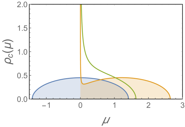
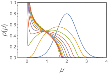
The Gaussian orthogonal ensemble (GOE), which was studied in Refs. Dean:2006wk ; DeanMajumdar , corresponds to ; then Eq. (51) gives for . The eigenvalue distribution for this case is shown by a green curve in Fig. 1.
The integral in Eq. (44) can be done by using the explicit forms of and . As a result we obtain
| (51) |
where
| (52) |
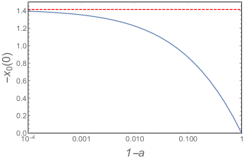
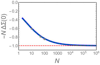
We can numerically solve Eq. (51) in terms of for given values of and . One is often interested in the case when , so that all eigenvalues are positive. In Fig. 2 we show as a function of for . We see that asymptotes to (as indicated by the red dashed line) for . To clarify the asymptotic behavior, we Taylor expand the function about . This gives
| (53) |
Now, to the leading order in , Eq. (51) becomes
| (54) |
where we have used that . Hence we find
| (55) |
For this gives
| (56) |
It is interesting to note that for and any value of . In this case Eq. (45) gives . This means that the distribution is just given by a shifted Wigner semi-circle (50) when we neglect the next-leading order correction in the large limit Bray:2007tf . Deviations from the Wigner semi-circle come from the next-leading order effect.
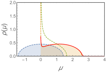
In the left panel of Fig. 3, we plot the eigenvalue distribution with for the case of (which corresponds to the Hessian distribution (22) and . We also plot the distribution for as an orange curve in Fig. 1, to compare it with the GOE distribution (plotted as a green curve). We see that the GOE distribution is much more concentrated near the origin, reflecting the high cost of a nonzero average eigenvalue in that case.
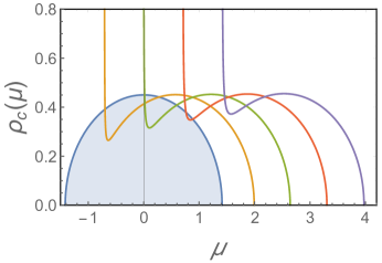
The Hessian distributions in Fig. 3 look like the Wigner semi-circle with an overall shift and a slight modification at the left edge. From Eqs. (45) and (56), the amount of the shift can be estimated as
| (57) |
for and in the limit of . The form of the distribution near the left edge, , where it significantly deviates from the Wigner semi-circle, can be found from Eqs. (46) and (56):
| (58) |
The number of eigenvalues in this range is
| (59) |
3.1.2 Probability of
The partition function can be approximated by its value at the saddle point:
| (60) |
Using Eq. (41), is given by
| (61) |
Here, the Lagrange multiplier can be determined from Eq. (41) by setting ,
| (62) | |||||
These integrals can be done explicitly by using Eq. (46). The result is
| (63) |
where we have used Eq. (44).
Since we are interested in the case where , we can simplify Eq. (63) by using Eq. (55). The result is
| (64) |
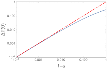
The probability for all eigenvalues to be greater than is given by , where and . This probability can be found numerically using Eqs. (44) and (63). In the right panel of Fig. 3, we plot as a function of . We also plot the asymptote in the limit of as a dashed red line. In the case of the Hessian distribution (22), , we obtain .333 This can be derived from the result of Ref. Bray:2007tf if we take a limit of , where is defined as a fraction of eigenvalues which are negative. However, their analysis is inaccurate in that limit. See also discussion below Eq. (86).
Now we can justify that the second term of in Eq. (39) gives a negligible contribution to in the large limit. As we already mentioned, this term is independent of the average eigenvalue . Furthermore, from Eq. (59) we see that the change in due to the modified distribution near is of the order . It follows that the contribution of the second term of to is , which is much smaller than the other terms in the large limit. We checked that it is indeed by numerically calculating as a function of with given by Eq. (46). Therefore, our result for is accurate with an uncertainty of . Additional support for neglecting the second term of comes from the fact that the distribution (46) obtained without this term agrees very well with the result of the dynamical method, which takes all terms into account (see Sec. 5).
4 Probability of at stationary points of the potential
We shall now calculate the probability for all Hessian eigenvalues to be greater than a given value at stationary points, where . For , this is the same as the probability for a stationary point to be a local minimum. We insert a delta function in Eq. (32) for the partition function to enforce the condition in the landscape:
| (65) |
The Jacobian () gives an additional factor for the probability distribution of the Hessian. Hence Eq. (30) should be replaced by
| (66) |
As we did in Sec. 3.1, we rescale the eigenvalues as and consider a density function of . In terms of this density function, we can rewrite as
| (67) | |||||
The partition function can also be expressed in terms of , as in Eq. (37), where is given by Eq. (38), while is now given by
We can absorb the third term in (LABEL:Sigma_1*) into the first term in the following way. To the leading order in , the distribution at the saddle point is the shifted Wigner semi-circle
| (69) |
Since is the next-leading order term, we can approximate it as . Then we can calculate the third term in (LABEL:Sigma_1*):
| (70) |
for . Using the definition
| (71) |
we can rewrite as
in the large limit. Therefore, we can use the result of the previous subsection, (51) and (63), with replaced by .
4.1 Probability of minima and the smallest eigenvalue
An important characteristic of a landscape is the density of potential minima in the field space. If the correlation length of the landscape is , the density of stationary points, where is – that is points per correlation volume. The density of minima can be obtained by multiplying this by the probability for a stationary point to be a local minimum. This is the same as the probability for all Hessian eigenvalues at that point to be positive,
| (73) |
where .
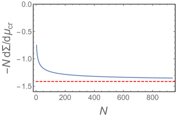
The left panel of Fig. 4 shows as a function of for the Hessian ensemble of Eq. (22), where is replaced by . It gets close to the asymptotic value () for , but significantly deviates from that value at smaller values of . The result can be well fitted by the following function, which is shown as the green dash-dotted line in the figure:
| (74) |
The probability has been studied earlier in the literature. Bray and Dean used the saddle point approximation in the large limit and found the asymptotic value Bray:2007tf . Easther et al EastherGuthMasoumi noted that can significantly deviate from this value for moderately large values of . They calculated the probability using efficient numerical codes for several values of up to . Their results, shown by grey dots in the left panel of Fig. 4, are in a very good agreement with ours. However, their fitting formula is not consistent with ours at larger values of . It is clear from the left panel of Fig. 4 that the asymptotic behavior cannot be correctly obtained by the extrapolation from .
For some applications it is important to estimate the smallest eigenvalue of the Hessian at potential minima (see, e.g., Sec. 6.2). The probability that this eigenvalue is greater than a given value can be found from
| (75) |
where now . For small values of we can approximate this as
| (76) |
The probability distribution for the smallest eigenvalue can then be estimated as
| (77) |
We plot at for the case of in the right panel of Fig. 4. We see that it is for and is asymptotic to at , as shown by the red dashed line, in agreement with the analytic formula (64). The typical magnitude of the smallest eigenvalue can now be estimated as
| (78) |
4.2 Probability of for a fixed
We shall now use the distribution (20) to calculate the probability for all Hessian eigenvalues to be greater than at a given value of . Eq. (20) can be rewritten as
where and we disregard terms that are independent of . We define shifted and rescaled eigenvalues and the parameter as
| (80) | |||
| (81) |
Then the resulting distribution for has the same form as Eq. (28).
The condition is equivalent to , where . Defining (), we obtain the relation between and the original threshold value :
| (82) |
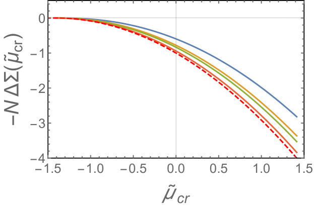
Thus we can use the same calculations and results as in Sec. 3 for the conditional probability at generic points in the landscape, with the replacements (81) and (82). In particular, when we are interested in the case where all eigenvalues are positive, we should set or . We plot as a function of for and in Fig. 5. The plots asymptote to the analytic formula (64) or
| (83) |
in the limit of , which is plotted as a red dashed line.
To calculate the probability for a stationary point at a given value of to have all Hessian eigenvalues greater than , we need to add a term in Eq. (30). Neglecting a constant term, the additional term can be written as . So we should replace and in Eq. (66). By using the argument around Eq. (69), we can replace the extra term by
in the leading order in the large limit, where and . As a result, we can rewrite as
| (85) |
If we redefine by shifting , this is the same as Eq. (LABEL:sigma1:stationaryP) and we can use the same calculation and result. Therefore, the term , which comes from the Jacobian for the stationary condition, gives two corrections: (as we discussed below Eq. (LABEL:sigma1:stationaryP)) and .
In summary, the probability for a stationary point at a given value of to have all Hessian eigenvalues greater than can be found from Eq. (83) with the above replacements:
| (86) |
A similar result has been derived by Bray and Dean in their Eq. (23) of Ref. Bray:2007tf , where their , , , , are our , , , , respectively. There is, however, a significant difference. Bray and Dean found the probability for a stationary point at a given value of to have a given index , where the index is defined as a fraction of eigenvalues which are negative. The average eigenvalue in their Eq. (23) has to be expressed in terms of through the relation
| (87) |
Their can be identified with our in the leading order approximation. We note, however, that Bray and Dean calculated only in the leading order in , which becomes rather inaccurate near the left edge of the distribution. Hence their result is not accurate for small values of . We do not have this problem in our calculation, so our result can be used for arbitrary values of .
We note also that even though the approximations we used here are sufficient for calculating , they are not accurate enough to find the distribution at small values of , because the distribution strongly deviates from the Wigner semi-circle near . In Sec. 5 we shall develop a new method which is sufficiently accurate in that regime.
5 Dynamical method
As we already noted, the approximations we used in Sections 4 and 4.1 are not sufficiently accurate for finding the eigenvalue distribution at small values of . In this section we develop a numerical method, using a version of the Dyson Brownian motion Dyson:1962 , to dynamically derive the distribution of Hessian eigenvalues. This method accounts for all terms in and without any approximations, apart from the limitations of numerical resolution and computer runtime. We shall first apply the Dyson Brownian motion method to the random matrix theory with GOE.
5.1 Random matrix theory
5.1.1 Dyson Brownian motion and Fokker-Planck equation
The Dyson Brownian motion model was introduced in Ref. Dyson:1962 to describe stochastic evolution of random matrices. The eigenvalues of a random matrix are assumed to undergo a stochastic process described by the Langevin equation
| (88) |
where is a stochastic variable,
| (89) |
The potential is given by
| (90) |
The eigenvalues are subject to a potential force and a stochastic force . Note that the potential is equal to the ‘Hamiltonian’ (30).
The probability density satisfies the Fokker-Planck equation, which can be obtained by taking the ensemble average over Dyson:1962 :
| (91) | |||
| (92) |
where and the potential force is given by
| (93) |
The equilibrium solution of Eq. (91) is given by the Boltzmann distribution,
| (94) |
Thus we can interpret and as the potential and the temperature, respectively. We note that the distribution (94) is the same as the eigenvalue distribution (29), (30) with for the GOE ensemble.
Since we are interested not in the individual variables , but in the distribution of eigenvalues, we define a time-dependent probability density as
| (95) |
We can easily check that . We also rescale the variable as to compare the results with those in Sec. 3. We set the normalization condition so we rescale the density . Then it obeys the following equation:
| (96) | |||
| (97) |
where is the temperature. The potential force is given by
| (98) |
where we have replaced the summation by the integral in the second term.
In what follows we shall use the Fokker-Planck equation for , without referring to the Langevin equation.
5.1.2 Dynamical evolution
We are interested in the equilibrium distribution under the condition that all eigenvalues are positive. This can be realized by evolving by Eq. (96) for a sufficiently long time444We note that the equilibrium eigenvalue distribution in a different class of models has been studied in Ref. Bachlechner:2012at , where they calculated the distribution by sampling the canonical ensemble with the Metropolis algorithm. with a reflecting boundary condition at ,
| (99) |
The equilibrium solution is stationary, , and it follows from Eq. (96) that . Then the boundary condition (99) requires that
| (100) |
This condition is similar to the one that we used to determine the saddle point solution (see Eq. (42)):
| (101) |
where we set . The first term in Eq. (101) comes from the term in , which we neglected in Sec.3. Thus Eq. (96) provides a useful check for the results of saddle point approximation.
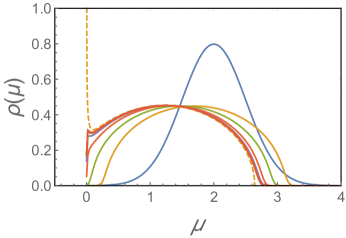
We solve the Fokker-Planck equation numerically by discretizing the differential equation. Numerical methods for solving the Fokker-Planck equation with the boundary condition (99) have been extensively studied Chang ; Mohammadi ; Pareschi . The grid size , the volume of -space , and the step size are taken to be , , and , respectively. We checked that our results are not affected by these parameters by varying their values. The results are presented in Fig. 6, where we take . The initial condition is taken to be a Gaussian function with a peak at and a width of , as indicated by a blue line. We see that the evolution converges to a stationary distribution, which agrees very well with the semi-analytic solution of Sec.3, with only a slight deviation at the right edge.
Here we comment on this slight deviation. It comes from the fact that we neglected the second term of in Eq. (39) to calculate the semi-analytic solution while we do not use any approximation to calculate in the dynamical method. To check that this deviation is physical and is consistent with the results in the literature, we calculated the distribution for the case of (i.e., for the case without the boundary) using the dynamical method. We found that the tails of the distribution at the right and left edges agree very well with the well-known Tracy-Widom distribution Tracy:1992rf ; Tracy:1995xi . Therefore, the smooth tail of the distribution at the right edge in Fig. 6 can be attributed to the spread of the largest eigenvalues a la Tracy-Widom beyond the edge of the semi-analytic distribution.
5.2 Hessian eigenvalue distribution in RGF model
The same method can be applied to find the Hessian eigenvalue distribution in a random Gaussian field, except in this case we should use in Eq. (30). Then the potential (90) is replaced by
| (102) |
and the potential force in the Fokker-Planck equation becomes
| (103) |
The equilibrium distribution is again equivalent to the saddle point solution of (42) with the term coming from included. We find this distribution by evolving via the Fokker-Planck equation.
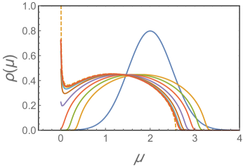
We solve the Fokker-Planck equation numerically and show the result in Fig. 7. We take and . The initial condition and other parameters are the same as we used in Sec.5.1.2 for the case of GOE. Once again, we see that the endpoint of the evolution is very close to the analytic solution. This justifies the approximation of neglecting the term in that we made in Sec. 4.
5.3 Hessian eigenvalue distribution at stationary points of the potential
We finally consider the Hessian eigenvalue distribution at stationary points, where , under the condition that all eigenvalues are positive. We found in Sec.4 that in this case has an additional term, . This adds an extra term to the potential force (103) in the Fokker-Planck equation,
| (104) |
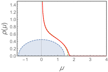
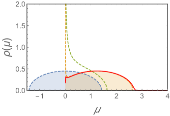
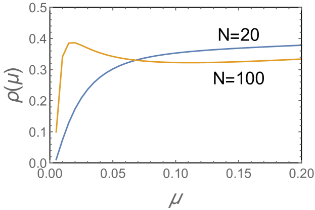
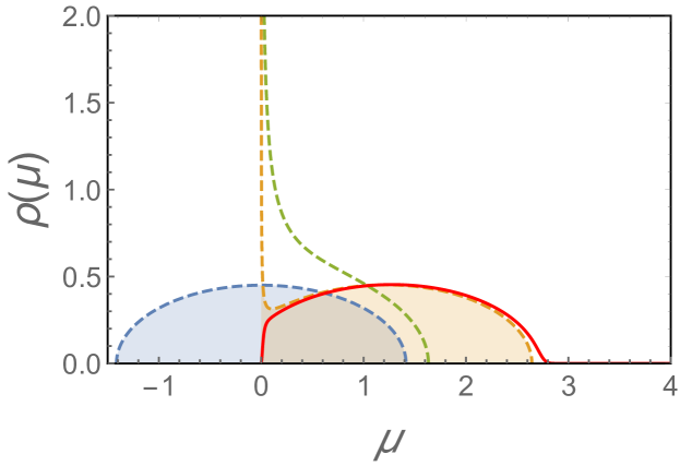
We solve the equation numerically using the same parameter values and initial condition as before. The results are presented in Fig. 8. The equilibrium distribution is shown by the solid shaded red line. For comparison we also show, by a dashed orange line, the semi-analytic distribution calculated in Sec. 4 for Hessian eigenvalues at generic points (not necessarily potential minima). We see that the two distributions are very close to one another, except near . The semi-analytic solution diverges as , while our equilibrium distribution drops sharply to zero. This is the effect of the strong repulsive force due to the last term in Eq. (104).
To illustrate the behavior of the distribution at small values of , we plot near for the cases of (blue line) and (yellow line) in Fig. 9. For , we can approximate , and Eq.(100) gives
| (105) |
with . This is in agreement with the plots in Fig. 9. We find that is about from our numerical results.
It should be noted, however, that our method may not be accurate in the range . The average number of eigenvalues in this range is , and thus replacing discrete eigenvalues by a continuous distribution is not justified.555We believe, however, that the sharp drop of the distribution to zero at is a real feature. A similar feature was found in Refs. MarcenkoPastur and Bachlechner:2012at , where the eigenvalue distribution was calculated for different models without using the continuous approximation. One can expect nevertheless that this approximation gives correct order-of-magnitude results near the limit of its applicability, . We can then use it to estimate the typical magnitude of the smallest eigenvalue of the Hessian, :
| (106) |
The plots in Fig. 9 suggests that for . Hence we find
| (107) |
The same estimate is obtained by numerically integrating the distribution in Eq. (106). It is in agreement with a more accurate estimate (78) in Sec. 4.1.
6 Some applications in cosmology
In this section we consider some applications of our result to the landscape models.
6.1 Vacuum stability
Vacuum stability in landscape models has been studied numerically in Refs. Greene:2013ida ; MV . A simple analytic treatment was given by Dine and Paban in Ref. Dine:2015ioa . They assume (i) that the most probable decay channels are typically in the directions of the smallest Hessian eigenvalues and (ii) that the vacuum decay rate is controlled mainly by the quadratic and cubic terms in the expansion of about the potential minimum. Then the tunneling (bounce) action in the direction of the Hessian eigenvalue can be estimated as
| (108) |
where is the typical coefficient of a cubic expansion term and is a numerical coefficient. The highest rate corresponds to the smallest Hessian eigenvalue . Dine and Paban assume that and find . With and , this can be rather small, , suggesting that most of the vacua in the landscape are very unstable.
A more accurate estimate of can be obtained from Eq. (78) or Eq. (107),
| (109) |
This corresponds to
| (110) |
and thus the tunneling action is
| (111) |
This is times larger than the estimate of Ref. Dine:2015ioa , so the vacuum stability is significantly enhanced. (We note that if we used Eq. (106) with the GOE eigenvalue distribution (Eq. (46) with ), we would have , which would suggest a much lower stability.)
6.2 Multi-field inflation
In this Section we assume that the landscape is small-field, which means that the correlation length is in Planck units. Slow-roll inflation in such a landscape occurs in rare flat regions, where the first and second derivatives of the potential in some direction are much smaller than their typical values. It was argued in Refs. MVY1 ; MVY2 ; MVY3 ; Blanco-Pillado:2017nin that inflation in such regions tends to be single-field, with the inflaton field rolling in a nearly straight line along the flat direction. Other fields (corresponding to orthogonal directions) can be excited and significant deviations from a straight trajectory can occur only if some of the fields have masses smaller than the Hubble parameter during inflation, in Planck units. This is much smaller than the typical mass . However, with a large number of fields some of the masses may be and may get as small as . We shall now investigate this possibility.
Flat inflationary tracks are likely to be found in the vicinity of inflection points, where one of the Hessian eigenvalues vanishes (this corresponds to the flat direction), the rest of the eigenvalues are positive, and the potential gradient vanishes in the directions orthogonal to the flat direction. Let us choose the axis in the flat direction. Then we have and , for . The mass spectrum in the directions orthogonal to the flat direction is determined by the Hessian eigenvalues, . We now want to estimate the smallest of these eigenvalues.
The probability distribution for Hessian eigenvalues at inflection points can be derived along the same lines as we derived Eq. (66). It is given by
| (112) | |||
| (113) |
This is similar to Eq. (66), but with a few differences. First, the coefficient of the last term is not unity but is . An additional term comes from the last term in parentheses of Eq. (66) with or . Second, the number of eigenvalues is .
We can now use the method of Sec. 4.1 to find the probability distribution for the second smallest Hessian eigenvalue at inflection points (the first smallest being ). We note that the number of eigenvalues is now and rewrite the coefficient of the second term in the parenthesis of (113) as , where , so this term becomes
| (114) |
As we explained in Sec. 4, the last term of Eq. (113) can be absorbed into by the replacement of , where the factor of comes from the coefficient of the last term. As a result, we should replace with in the calculation of Sec. 3.1. Since , the result should be the same with the one obtained in Sec. 4 in the large limit. Therefore the distribution of eigenvalues at an inflection point is given by with and . The probability for all eigenvalues to be positive is given by , and the typical value of can be estimated as in Eq. (78),
| (115) |
The asymptotic value of is in the limit .
The distribution of eigenvalues at inflection points can be found using the dynamical method of Sec. 5. The Fokker-Planck equation has the same form as before, but with slightly different parameters and coefficients. The temperature in Eq. (97) is given by and the potential force is given by
| (116) |
where . The change in the last term of modifies the form of the distribution at . In this limit, the Fokker-Planck equation reduces to , with the solution
| (117) |
where .
The distribution obtained by numerically evolving the Fokker-Planck equation is shown in Fig. 10. We find that the constant in Eq. (117) is from our numerical results. As in Sec. 5.3, the average number of eigenvalues in the range is , so we cannot expect our distribution to be accurate in this range.
As before, the second smallest eigenvalue of the Hessian, , can also be estimated from
| (118) |
which gives
| (119) |
in agreement with (115).
The rescaled eigenvalue (119) corresponds to . If this is smaller than about , then the associated field will undergo significant fluctuations and may play a dynamical role during inflation. This is unlikely if . Thus we conclude that multifield inflation is not likely for (for ).
7 Conclusions
The main focus of this paper was to investigate the Hessian eigenvalue distribution at local minima of a random Gaussian landscape. Bray and Dean used the saddle point approximation to calculate this distribution and the density of local minima in the leading order of the large expansion. We found, however, that the next-to-leading order corrections modify the distribution at the lower edge of the domain. This is particularly important for the smallest Hessian eigenvalues, which we need to estimate for assessing the vacuum stability and the multi-field nature of inflation in the landscape.
We extended the saddle point method to account for the sub-leading in contributions and used it to calculate the density of local minima in the landscape. This method can also be used to determine the Hessian eigenvalue distribution at a generic point in the landscape, but it fails to find the distribution at potential minima with the desired accuracy. For that we had to develop a completely new approach.
In our new approach, the Hessian eigenvalue distribution is calculated as the asymptotic endpoint of a stochastic process, called Dyson Brownian motion. The distribution is evolved via a suitable Fokker-Planck equation, and the equilibrium distribution is obtained after a sufficiently large number of iterations. We have verified that this method agrees with the saddle point method in cases where the latter method is applicable.
We discussed some implications of our results for vacuum stability and slow-roll inflation in the landscape. We found that metastable vacua in a Gaussian landscape are more stable than a naive estimate would suggest. Slow-roll inflation at inflection points in the landscape is likely to be single-field when the smallest nonzero Hessian eigenvalue at a typical inflection point is greater than the energy scale of the landscape . We found that this condition is satisfied if the correlation length in the landscape is . For , this means that inflation is essentially single-field in a landscape with in Planck units.
In Appendix A we discussed the relation between a random Gaussian landscape and an axionic landscape. We specified the conditions under which an axionic landscape can be approximated by an isotropic random Gaussian field. We expect that our results should be applicable to such axion models.
We note finally that the problem of Hessian eigenvalue distribution in a random field arises in many areas of condensed matter physics (see, e.g., Beenakker:1997 ; Guhr:1997ve ; Eynard:2015aea and references therein). Our methods and results may be useful in these areas as well.
Acknowledgments
We would like to thank Jose J. Blanco-Pillado for useful conversations and Thomas Bachlechner and Yan V. Fyodorov for their useful comments on the manuscript. This work was supported in part by the National Science Foundation under grant 1518742.
Appendix A Axion landscape
In this Appendix we extend the argument of Ref. Bachlechner:2017hsj to show that under certain conditions the axion landscape can be approximately described by an isotropic random Gaussian field model.
Axions develop a periodic potential due to non-perturbative effects. (For a review of axions see, e.g., Kim:2008hd .) In general the potential has the form
| (120) |
where
| (121) |
are the energy scales of non-perturbative effects, is an -component vector, its components being the axion fields, is a vector with integer components , and are periodic functions with a period ,
| (122) |
The phase constants are assumed to be random parameters with a flat distribution in the range from to , and are independent random variables with a specified distribution . Following Ref. Bachlechner:2017hsj , we shall assume for simplicity that all these distributions are identical: (although this can be easily generalized).
Since the functions are periodic, they can be represented as
| (123) |
with . In Ref. Bachlechner:2017hsj , they assume , in which case , , and for all . In what follows, we consider a generic periodic function . For example, the strong dynamics of QCD results in a complicated periodic function for the QCD axion DiVecchia:1980yfw (see also Ref. diCortona:2015ldu for a recent work).
String theory predicts the existence of a large number of axions, (e.g., Svrcek:2006yi ). In Ref. Bachlechner:2017hsj it was shown that interesting alignment effects can arise in the axionic landscape if the number of terms in the potential (120) is . They also noted that for the potential approaches that for a random Gaussian field, as a consequence of the central limit theorem. The statistical properties of this field depend on the choice of the distribution .
The integers define a lattice in the -space with a spacing . We shall assume that the variance of the distribution is , which means that the correlation length of is small compared to the periodicity length . Then the distribution can be approximated as continuous.
We will be interested in the two-point correlation function for the potential . After averaging over the random phases, this function should depend only on the difference . Then, without loss of generality, we can choose one of the points to be at . Thus, we consider
| (124) |
where () represents the ensemble average over random variables . We use
| (125) |
and
| (126) |
where
| (127) |
Substituting this in (124), we have
| (128) |
Now we consider some possible forms of . The first is
| (129) |
In this case, the combined distribution for all components is
| (130) |
This depends only on and thus is rotationally invariant in the -space. Note that Eq. (130) is the only factorized distribution, , that has this property. We can expect the two-point function to also be rotationally invariant in the -space. Indeed, from Eq. (127) we have
| (131) |
Since we assume that , the sum over can be approximated by an integral, so we obtain
| (132) |
and
| (133) |
Note that if depends on the index , in this equation should simply be replaced by .
Now let us consider the form of , which was adopted in Ref. Bachlechner:2017hsj : for and otherwise. In this case,
| (134) |
Hence,
| (135) |
Unlike Eq. (133), this correlation function is not rotationally invariant. The reason is that rotational invariance is violated by the probability distribution for .
It may be instructive to compare the correlators of the potential and its derivatives for different choices of . We find
| (136) | |||
| (137) | |||
| (138) | |||
| (139) |
where primes denote derivatives with respect to . The gradient is not correlated with the potential nor the Hessian. The ensemble average over gives
| (140) | |||
| (141) | |||
| (142) |
where is the variance of random variable .
If we identify
| (143) | |||
| (144) | |||
| (145) |
we see that the resulting correlation functions have the same form as Eqs. (6)-(10), except for the additional term () in (141). This additional term breaks the rotational invariance of the model and vanishes when the random variables have a rotationally invariant distribution (130). In Ref. Bachlechner:2017hsj , the authors assumed a flat distribution for as an example (which breaks rotational invariance) and obtained .
The extra term in (141) also indicates a deviation from Gaussian statistics. However, it affects only the statistics of the diagonal components of the Hessian. There are only diagonal components and non-diagonal ones, so we can expect this term to be unimportant at large . The same discussion applies to correlators for higher-order derivatives. Thus we expect that Gaussian random fields give a good approximation for this type of landscape in the limit of and .
Finally, we comment that the cancellation for the coefficient of () occurs when , which was adopted in Ref. Bachlechner:2017hsj . In this case, the Hessian distribution is just given by the GOE with a constant shift of the diagonal terms as Eq. (27). However, this is not a generic property of axion landscape with a generic choice of functions .
References
- (1) R. Bousso and J. Polchinski, “Quantization of four form fluxes and dynamical neutralization of the cosmological constant,” JHEP 0006, 006 (2000) [hep-th/0004134].
- (2) L. Susskind, “The Anthropic landscape of string theory,” In *Carr, Bernard (ed.): Universe or multiverse?* 247-266 [hep-th/0302219].
- (3) A. Linde, “A brief history of the multiverse,” Rept. Prog. Phys. 80, no. 2, 022001 (2017) [arXiv:1512.01203 [hep-th]].
- (4) M. Tegmark, “What does inflation really predict?,” JCAP 0504, 001 (2005) [astro-ph/0410281].
- (5) A. Aazami and R. Easther, “Cosmology from random multifield potentials,” JCAP 0603, 013 (2006) [hep-th/0512050].
- (6) J. Frazer and A. R. Liddle, “Exploring a string-like landscape,” JCAP 1102, 026 (2011) [arXiv:1101.1619 [astro-ph.CO]].
- (7) D. Battefeld, T. Battefeld and S. Schulz, “On the Unlikeliness of Multi-Field Inflation: Bounded Random Potentials and our Vacuum,” JCAP 1206, 034 (2012) [arXiv:1203.3941 [hep-th]].
- (8) T. C. Bachlechner, D. Marsh, L. McAllister and T. Wrase, “Supersymmetric Vacua in Random Supergravity,” JHEP 1301, 136 (2013) [arXiv:1207.2763 [hep-th]].
- (9) I. S. Yang, “Probability of Slowroll Inflation in the Multiverse,” Phys. Rev. D 86, 103537 (2012) [arXiv:1208.3821 [hep-th]].
- (10) T. C. Bachlechner, “On Gaussian Random Supergravity,” JHEP 1404, 054 (2014) [arXiv:1401.6187 [hep-th]].
- (11) G. Wang and T. Battefeld, “Vacuum Selection on Axionic Landscapes,” JCAP 1604, no. 04, 025 (2016) arXiv:1512.04224 [hep-th]..
- (12) A. Masoumi and A. Vilenkin, “Vacuum statistics and stability in axionic landscapes,” JCAP 1603, no. 03, 054 (2016) [arXiv:1601.01662 [gr-qc]].
- (13) R. Easther, A. H. Guth and A. Masoumi, “Counting Vacua in Random Landscapes,” arXiv:1612.05224 [hep-th].
- (14) A. Masoumi, A. Vilenkin and M. Yamada, “Inflation in random Gaussian landscapes,” JCAP 1705, no. 05, 053 (2017) arXiv:1612.03960 [hep-th].
- (15) A. Masoumi, A. Vilenkin and M. Yamada, “Initial conditions for slow-roll inflation in a random Gaussian landscape,” JCAP 1707, no. 07, 003 (2017) arXiv:1704.06994 [hep-th].
- (16) A. Masoumi, A. Vilenkin and M. Yamada, “Inflation in multi-field random Gaussian landscapes,” arXiv:1707.03520 [hep-th].
- (17) T. Bjorkmo and M. C. D. Marsh, “Manyfield Inflation in Random Potentials,” arXiv:1709.10076 [astro-ph.CO].
- (18) J. J. Blanco-Pillado, A. Vilenkin and M. Yamada, “Inflation in Random Landscapes with two energy scales,” arXiv:1711.00491 [hep-th].
- (19) J. E. Kim, H. P. Nilles and M. Peloso, “Completing natural inflation,” JCAP 0501, 005 (2005) [hep-ph/0409138].
- (20) S. Dimopoulos, S. Kachru, J. McGreevy and J. G. Wacker, “N-flation,” JCAP 0808, 003 (2008) [hep-th/0507205].
- (21) L. McAllister, E. Silverstein and A. Westphal, “Gravity Waves and Linear Inflation from Axion Monodromy,” Phys. Rev. D 82, 046003 (2010) [arXiv:0808.0706 [hep-th]].
- (22) T. Higaki and F. Takahashi, “Natural and Multi-Natural Inflation in Axion Landscape,” JHEP 1407, 074 (2014) [arXiv:1404.6923 [hep-th]].
- (23) G. Wang and T. Battefeld, “Vacuum Selection on Axionic Landscapes,” JCAP 1604, no. 04, 025 (2016) [arXiv:1512.04224 [hep-th]].
- (24) T. C. Bachlechner, K. Eckerle, O. Janssen and M. Kleban, “Systematics of Aligned Axions,” arXiv:1709.01080 [hep-th].
- (25) A. J. Bray and D. S. Dean, “Statistics of critical points of Gaussian fields on large-dimensional spaces,” Phys. Rev. Lett. 98, 150201 (2007).
- (26) Y. V. Fyodorov and C. Nadal, “Critical Behavior of the Number of Minima of a Random Landscape at the Glass Transition Point and the Tracy-Widom Distribution,” Phys. Rev. Lett. 106, 167203 (2012) [arXiv:1207.6790 [cond-mat]].
- (27) Y. V. Fyodorov and I. Williams, "Replica Symmetry Breaking Condition Exposed by Random Matrix Calculation of Landscape Complexity," J. Stat. Phys. 129, 1081 (2007) [arXiv:cond-matt/0702601]
- (28) F. J. Dyson “A Brownian-Motion Model for the Eigenvalues of a Random Matrix,” J. Math. Phys. 3 (Nov., 1962), 1191-1198.
- (29) Y. V. Fyodorov, "Complexity of random energy landscapes, glass transition and absolute value of spectral determinant of random matrices," Phys. Rev. Letters 92, 240601 (2004).
- (30) E. P. Wigner, “Characteristic Vectors of Bordered Matrices With Infinite Dimensions,” Annals of Mathematics, 62(3), 548-564 (1955).
- (31) D. S. Dean and S. N. Majumdar, “Large deviations of extreme eigenvalues of random matrices,” Phys. Rev. Lett. 97, 160201 (2006) [cond-mat/0609651].
- (32) D. S. Dean and S. N. Majumdar, “Extreme value statistics of eigenvalues of Gaussian random matrices,” Phys. Rev. E 77, 041108 (2008) [arXiv:0801.1730 [cond-mat.stat-mech]].
- (33) J.S. Chang, G. Cooper, “A practical difference scheme for Fokker-Planck equations,” In Journal of Computational Physics, Volume 6, Issue 1, 1970, Pages 1-16, ISSN 0021-9991.
- (34) M. Mohammadi, and A. Borzì, “Analysis of the Chang–Cooper discretization scheme for a class of Fokker–Planck equations,” Journal of Numerical Mathematics, 23(3), pp. 271-288. (2015).
- (35) L. Pareschi and M. Zanella, “Structure preserving schemes for nonlinear Fokker-Planck equations and applications,” arXiv:1702.00088 [math.NA].
- (36) C. A. Tracy and H. Widom, “Level spacing distributions and the Airy kernel,” Commun. Math. Phys. 159, 151 (1994) [hep-th/9211141].
- (37) C. A. Tracy and H. Widom, “On orthogonal and symplectic matrix ensembles,” Commun. Math. Phys. 177, 727 (1996) [solv-int/9509007].
- (38) V. A. Marcenko and L. A. Pastur, “DISTRIBUTION OF EIGENVALUES FOR SOME SETS OF RANDOM MATRICES,” Mathematics of the USSR-Sbornik 1, no. 4, 457 (1967).
- (39) B. Greene, D. Kagan, A. Masoumi, D. Mehta, E. J. Weinberg and X. Xiao, “Tumbling through a landscape: Evidence of instabilities in high-dimensional moduli spaces,” Phys. Rev. D 88, no. 2, 026005 (2013) [arXiv:1303.4428 [hep-th]].
- (40) M. Dine and S. Paban, “Tunneling in Theories with Many Fields,” JHEP 1510, 088 (2015) [arXiv:1506.06428 [hep-th]].
- (41) C. W. J. Beenakker, “Random-matrix theory of quantum transport,” Rev. Mod. Phys. 69, 731 (1997) [cond-mat/9612179].
- (42) T. Guhr, A. Muller-Groeling and H. A. Weidenmuller, “Random matrix theories in quantum physics: Common concepts,” Phys. Rept. 299, 189 (1998) [cond-mat/9707301].
- (43) B. Eynard, T. Kimura and S. Ribault, “Random matrices,” arXiv:1510.04430 [math-ph].
- (44) J. E. Kim and G. Carosi, “Axions and the Strong CP Problem,” Rev. Mod. Phys. 82, 557 (2010) [arXiv:0807.3125 [hep-ph]].
- (45) P. Svrcek and E. Witten, “Axions In String Theory,” JHEP 0606, 051 (2006) [hep-th/0605206].
- (46) P. Di Vecchia and G. Veneziano, “Chiral Dynamics in the Large n Limit,” Nucl. Phys. B 171, 253 (1980).
- (47) G. Grilli di Cortona, E. Hardy, J. Pardo Vega and G. Villadoro, “The QCD axion, precisely,” JHEP 1601, 034 (2016) [arXiv:1511.02867 [hep-ph]].