${SO(10)}$ inspired $Z^{\prime}$ models at the LHC

Abstract

We study and compare various $Z^{\prime}$ models arising from $SO(10)$, focussing in particular on the Abelian subgroup $U(1)_{R}\times U(1)_{B-L}$, broken at the TeV scale to Standard Model hypercharge $U(1)_{Y}$. The gauge group $U(1)_{R}\times U(1)_{B-L}$, which is equivalent to the $U(1)_{Y}\times U(1)_{\chi}$ in a different basis, is well motivated from $SO(10)$ breaking and allows neutrino mass via the linear seesaw mechanism. Assuming supersymmetry, we consider single step gauge unification to predict the gauge couplings, then consider the detection and characterisation prospects of the resulting $Z^{\prime}$ at the LHC by studying its possible decay modes into di-leptons as well as into Higgs bosons. The main new result here is to analyse in detail the expected leptonic forward-backward asymmetry at the high luminosity LHC and show that it may be used to discriminate the $U(1)_{R}\times U(1)_{B-L}$ model from the usual $B-L$ model based on $U(1)_{Y}\times U(1)_{B-L}$.

I Introduction

$SO(10)$ Grand Unified Theories (GUTs) are very attractive since they predict right-handed neutrinos and make neutrino mass inevitable. Supersymmetry (SUSY) allows for a single step unification of the gauge couplings. Being a rank 5 gauge group, $SO(10)$ also naturally accommodates an additional $Z^{\prime}$ gauge boson, which may have a mass at the TeV scale within the range of the Large Hadron Collider (LHC). Such $Z^{\prime}$ models are attractive since, apart from the three right-handed neutrinos, they do not require any new exotic particles to make the theory anomaly free.

There are two main symmetry breaking patterns of $SO(10)$ leading to the Standard Model (SM) gauge group. Firstly there is the $SU(5)$ embedding,

$$SO(10)\rightarrow SU(5)\times U(1)_{\chi}\rightarrow SU(3)_{C}\times SU(2)_{L}\times U(1)_{Y}\times U(1)_{\chi}$$ (1)

where the $U(1)_{\chi}$ is broken at the TeV scale, yielding a massive $Z^{\prime}_{\chi}$. For recent examples of models based on such a $Z^{\prime}_{\chi}$, see e.g. King:2017anf .

Secondly there is the Pati-Salam gauge group embedding,

$$SO(10)\rightarrow SU(4)_{PS}\times SU(2)_{L}\times SU(2)_{R}$$ (2)

The Pati-Salam colour group $SU(4)_{PS}$ may be broken to $SU(3)_{C}\times U(1)_{B-L}$, leading to the left-right symmetric model gauge group. The $SU(2)_{R}$ group may be broken to the gauge group $U(1)_{R}$ associated with the diagonal generator $T_{3R}$. It is thus possible to break $SO(10)$ in a single step at the GUT scale without reducing the rank,

$$SO(10)\rightarrow SU(3)_{C}\times SU(2)_{L}\times U(1)_{R}\times U(1)_{B-L}$$ (3)

The resulting gauge group in Eq.3 does not predict any new charged currents and is not very tightly constrained phenomenologically. It may therefore survive down to the TeV scale before being broken to the SM gauge group, leading to the prediction of a massive $Z^{\prime}_{BLR}$, accessible to the Large Hadron Collider (LHC).

In this paper we shall focus on $SO(10)$ broken at the GUT scale in a single step, as in Eq.3. In order to allow for gauge coupling unification we shall assume supersymmetry (SUSY) which is broken close to the TeV scale, but at a high enough scale to enable the superpartners to have evaded detection at the LHC. We shall be interested in the $Z^{\prime}_{BLR}$ which emerges when the Abelian subgroup $U(1)_{R}\times U(1)_{B-L}$ is broken down to the SM hypercharge gauge group $U(1)_{Y}$ near the TeV scale (for brevity we refer to this scenario as the BLR model). We study the discovery prospects of such a $Z^{\prime}_{BLR}$ at the LHC, its possible decay mode into Higgs bosons, and the expected forward-backward asymmetry, comparing the predictions to the well studied $B-L$ model based on $U(1)_{Y}\times U(1)_{B-L}$ King:2004cx ; Khalil:2007dr ; FileviezPerez:2010ek ; OLeary:2011vlq ; Elsayed:2011de . We comment on the $U(1)_{Y}\times U(1)_{\chi}$ model Arcadi:2017atc ; Accomando:2010fz below.

The Abelian gauge group $U(1)_{R}\times U(1)_{B-L}$ has quite a long history in the literature as reviewed in Langacker:2008yv ; Accomando:2010fz . It was recently realised that SUSY $SO(10)$ models which break down to this gauge group may allow for a new type of seesaw model, namely the linear seesaw model Malinsky:2005bi ; Hirsch:2009mx . Subsequently, the phenomenology of the SUSY $U(1)_{R}\times U(1)_{B-L}$ model has been studied in a number of works DeRomeri:2011ie ; Hirsch:2011hg ; Hirsch:2012kv ; Basso:2012ew ; Frank:2017ohg ; Chakrabortty:2009xm ; Krauss:2013jva . Indeed it has been demonstrated that the Abelian BLR gauge group $U(1)_{R}\times U(1)_{B-L}$ is equivalent to $U(1)_{Y}\times U(1)_{\chi}$ (arising from the breaking chain in Eq.1) by a basis transformation and furthermore that this equivalence is preserved under RGE running, when kinetic mixing is consistently taken into account Krauss:2013jva . Therefore the physics of the TeV scale $Z^{\prime}_{BLR}$ considered here should be identical to that of the $Z^{\prime}_{\chi}$ Krauss:2013jva .

We emphasise that there are several new aspects of our study including: the statistical significance of producing a $Z^{\prime}_{BLR}$ at the LHC including finite width and interference effects (the LHC uses a narrow width approximation); the study of Higgs final states in the $U(1)_{B-L}\times U(1)_{R}$ model; and the study of forward-backward asymmetry at the high luminosity LHC as a discriminator between the $U(1)_{R}\times U(1)_{B-L}$ model (or equivalently the $U(1)_{Y}\times U(1)_{\chi}$ model) and the usual $Z^{\prime}_{BL}$ based on $U(1)_{Y}\times U(1)_{B-L}$, i.e. the commonly studied $B-L$ model King:2004cx ; Khalil:2007dr ; FileviezPerez:2010ek ; OLeary:2011vlq ; Elsayed:2011de .

The layout of the remainder of the paper is as follows. In section II we discuss the BLR model. In section III we give the $Z^{\prime}_{BLR}$ couplings to fermions in this model, while in section IV we give the $Z^{\prime}_{BLR}$ couplings to Higgs. In section V we present a renormalisation group analysis of the BLR model. In section VI we present the results for the Drell-Yan production of the $Z^{\prime}$ in the BLR model, assessing the discovery potential at the LHC, present the leptonic forward-backward asymmetry as a discriminator of different models, and discuss the Higgs final state branching fractions of $Z^{\prime}_{BLR}$ decays. Section VII concludes the paper.

II Model

We shall not consider the high energy $SO(10)$ breaking here, so the starting point of the considered model is to assume that, below the GUT scale, we have the gauge group as on the right-hand side of Eq.3, namely,

$$SU(3)_{C}\times SU(2)_{L}\times U(1)_{R}\times U(1)_{B-L}$$ (4)

Note that in this basis the hypercharge gauge group $U(1)_{Y}$ of the SM is not explicitly present, instead it is “unified” into $U(1)_{R}\times U(1)_{B-L}$. Note that, although the Abelian factors are equivalent to the $U(1)_{Y}\times U(1)_{\chi}$ model by a basis transformation, we shall work in the $U(1)_{R}\times U(1)_{B-L}$ basis. In order to allow gauge coupling unification we need SUSY, but we shall assume it is broken above the $Z^{\prime}_{BLR}$ mass scale so that SUSY particles are not present in the decays of the $Z^{\prime}_{BLR}$. Note that such SUSY decays have been considered extensively in DeRomeri:2011ie ; Hirsch:2011hg ; Hirsch:2012kv ; Basso:2012ew ; Frank:2017ohg ; Chakrabortty:2009xm ; Krauss:2013jva .

At the $Z^{\prime}_{BLR}$ mass scale (typically a few TeV), hypercharge emerges from the breaking,

$$U(1)_{R}\times U(1)_{B-L}\rightarrow U(1)_{Y}$$ (5)

where the hypercharge generator is identified as

$$Y=T_{3R}+T_{B-L},$$ (6)

where

$$T_{B-L}=(B-L)/2.$$ (7)

The symmetry breaking in Eq.5 requires two Higgs superfields $\chi_{1,2}$ whose scalar components develop Vacuum Expectation Values (VEVs) which carry non-zero $T_{3R}$ and opposite $T_{B-L}$ so that they are neutral under hypercharge. If they arise from an $SU(2)_{R}$ doublet then this fixes their charges to be $T_{3R}=\pm 1/2$ and hence $T_{B-L}=\mp 1/2$. Two of them with opposite quantum numbers are required by SUSY to cancel anomalies (and for holomorphicity). They must be singlets under both $SU(3)_{C}$ and $SU(2)_{L}$ in order to preserve these gauge groups.

Finally, at the electroweak (EW) scale we have the usual Standard Model (SM) breaking

$$SU(2)_{L}\times U(1)_{Y}\rightarrow U(1)_{Q},$$ (8)

where the electric charge generator is identified as

$$Q=T_{3L}+Y.$$ (9)

As in usual SUSY models, the EW symmetry breaking is accomplished by two Higgs doublets $H_{u,d}$ of $SU(2)_{L}$ which have $B-L=0$. If the two Higgs doublets of $SU(2)_{L}$ were embedded into a single $SU(2)_{R}$ doublet, then we expect that $H_{u,d}$ will have $T_{3R}=\pm 1/2$, respectively. In addition, in order to accomplish neutrino masses via the linear seesaw model, we need to add three complete singlet superfields $S$, as discussed in the appendix A. The particle content of the model (henceforth denoted as BLR) is then summarised in Tab. 1.

Particle	$T_{3L}$	$T_{3R}$	$T_{B-L}$	$T_{\chi}$	$Y=T_{3R}+T_{B-L}$	$Q=T_{3L}+Y$
$\begin{pmatrix}u\\ d\end{pmatrix}_{L}$	+1/2	0	+1/6	+1/4	+1/6	+2/3
	-1/2	0	+1/6	+1/4	+1/6	-1/3
$u_{R}$	0	+1/2	+1/6	-1/4	+2/3	+2/3
$d_{R}$	0	-1/2	+1/6	+3/4	-1/3	-1/3
$\begin{pmatrix}\nu_{e}\\ e^{-}\end{pmatrix}_{L}$	+1/2	0	-1/2	-3/4	-1/2	0
	-1/2	0	-1/2	-3/4	-1/2	-1
$\nu_{R}$	0	+1/2	-1/2	-5/4	0	0
$e_{R}$	0	-1/2	-1/2	-1/4	-1	-1
$\chi_{R}^{1}$	0	-1/2	+1/2	+5/4	0	0
$\chi_{R}^{2}$	0	+1/2	-1/2	-5/4	0	0
$S$	0	0	0	0	0	0
$H\begin{cases}H_{u}=\begin{pmatrix}\phi_{u}^{+}\\ \phi_{u}^{0}\end{pmatrix}_{L}\\[-10.00002pt] \\ H_{d}=\begin{pmatrix}\phi_{d}^{0}\\ \phi_{d}^{-}\end{pmatrix}_{L}\end{cases}$	+1/2	+1/2	0	-1/2	+1/2	+1
	-1/2	+1/2	0	-1/2	+1/2	0
	+1/2	-1/2	0	+1/2	-1/2	0
	-1/2	-1/2	0	+1/2	-1/2	-1

Table 1: The particle content and generators of the $SU(3)_{C}\times SU(2)_{L}\times U(1)_{R}\times U(1)_{B-L}$ model.

III $Z^{\prime}$ couplings to fermions

In this work, numerically, we use the SARAH program Staub:2013tta to determine the vector and axial couplings of the fermions with the $Z^{\prime}_{BLR}$. This includes the full impact of Gauge-Kinetic Mixing (GKM) as done in Hirsch:2012kv ; Krauss:2013jva . Considering this effect in full leads to $\sim\mathcal{O}(1)\%$ differences in vector and axial couplings. In this section, for simplicity, we neglect the impact of GKM but stress that all implications are considered in our final results.

We begin by examining the low energy breaking of the gauge group in Eq.5. The coupling of a fermion $f$ to the $U(1)_{R}$ and $U(1)_{B-L}$ fields are obtained from

$$-\mathcal{L}_{\rm BLR}=\bar{f}\gamma^{\mu}\left(g_{R}T_{3R}W^{3}_{\mu R}+g_{BL}T_{B-L}B^{BL}_{\mu}\right)f,$$ (10)

where $T_{B-L}=\frac{B-L}{2}$.

After symmetry breaking, these two fields will mix to become the SM massless hypercharge gauge boson, $B_{\mu}$, and a massive $Z^{\prime}_{\mu}$ (corresponding to the $Z^{\prime}_{BLR}$),

$$\begin{pmatrix}B^{BL}_{\mu}\\ W^{3}_{\mu R}\\ \end{pmatrix}=\begin{pmatrix}\cos\theta_{BL}&-\sin\theta_{BL}\\ \sin\theta_{BL}&\cos\theta_{BL}\\ \end{pmatrix}\begin{pmatrix}B_{\mu}\\ Z^{\prime}_{\mu}\end{pmatrix}.$$ (11)

So, the $Z^{\prime}_{BLR}$ has the following coupling to fermions:

$$-\mathcal{L}^{Z^{\prime}}_{\rm BLR}=Z^{\prime}_{\mu}\bar{f}\gamma^{\mu}\left(g_{R}\cos\theta_{BL}T_{3R}-g_{BL}\sin\theta_{BL}T_{B-L}\right)f.$$ (12)

Since

$$g_{R}\sin\theta_{BL}=g_{BL}\cos\theta_{BL}=g_{Y},$$ (13)

we may rewrite the $Z^{\prime}$ couplings of the BLR model in a more compact form,

$$-\mathcal{L}^{Z^{\prime}}_{\rm BLR}=Z^{\prime}_{\mu}\bar{f}\gamma^{\mu}g_{Y}Q_{LR}f,$$

$$Q_{LR}\equiv\left(\cot\theta_{BL}T_{3R}-\tan\theta_{BL}T_{B-L}\right),\ \ \ \tan\theta_{BL}=g_{BL}/g_{R}.$$ (14)

We shall be interested in comparing the $Z^{\prime}$ couplings in the BLR model above to those in related models where the SM gauge group (including hypercharge) is augmented by an Abelian gauge group $U(1)^{\prime}$, identified with the generator $T_{BL}$, resulting in the $Z^{\prime}$ couplings

$$-\mathcal{L}^{Z^{\prime}}_{BL}=Z^{\prime}_{\mu}\bar{f}\gamma^{\mu}g_{BL}T_{B-L}f,$$ (15)

which may be compared to the BLR couplings in Eq.14. We shall find to one-loop the non-GUT normalised couplings (i.e., in the conventions of this section):

$$g_{R}=0.448,\ \ g_{BL}=0.459.\ \$$ (16)

In general the $Z^{\prime}_{BLR}$ couples to a fermion $f$ which may be either left- or right-handed and the above couplings sum over both chiral components of all the fermions. For analysing the couplings of different models it is useful to decompose the couplings into either left-chiral or right-chiral components, leading to the vector and axial couplings in the BLR model as follows

$$-\mathcal{L}^{Z^{\prime}}_{\rm BLR}=g_{Y}Z^{\prime}_{\mu}\bar{f}\gamma^{\mu}(\epsilon_{L}^{f}P_{L}+\epsilon_{R}^{f}P_{R})f=g_{Y}Z^{\prime}_{\mu}\bar{f}\gamma^{\mu}\frac{1}{2}\left({g_{V}^{f}-g_{A}^{f}\gamma^{5}}\right)f,$$ (17)

where $P_{R,L}=(1\pm\gamma_{5})/2$ and the vector/axial couplings are defined as $g_{V/A}^{f}=\epsilon_{L}^{f}\pm e_{R}^{f}$. Similar decompositions can be made for the $Z^{\prime}$ couplings of the other models in Eq.15. Tab. 2 shows the chiral couplings for the relevant generators $T_{R}$ and $T_{B-L}=(B-L)/2$. Tab. 3 shows the vector and axial couplings obtained for the two different models.

Model	$\epsilon_{L}^{u}$	$\epsilon_{R}^{u}$	$\epsilon_{L}^{d}$	$\epsilon_{R}^{d}$	$\epsilon_{L}^{e}$	$\epsilon_{R}^{e}$	$\epsilon_{L}^{\nu}$	$\epsilon_{R}^{\nu}$
$T_{3R}$	$0$	$1/2$	$0$	$-1/2$	$0$	$-1/2$	$0$	$1/2$
$T_{B-L}$	$1/6$	$1/6$	$1/6$	$1/6$	$-1/2$	$-1/2$	$-1/2$	$-1/2$

Table 2: Chiral couplings for the $U(1)_{R}$ and $U(1)_{B-L}$ models.

Model	$g_{V}^{u}$	$g_{A}^{u}$	$g_{V}^{d}$	$g_{A}^{d}$	$g_{V}^{e}$	$g_{A}^{e}$	$g_{V}^{\nu}$	$g_{A}^{\nu}$
$T_{3R}$	$1/2$	$-1/2$	$-1/2$	$1/2$	$-1/2$	$1/2$	$0$	$0$
$T_{B-L}$	$1/3$	$0$	$1/3$	$0$	$-1$	$0$	$-1/2$	$-1/2$

Table 3: Vector and axial couplings for the $U(1)_{R}$ and $U(1)_{B-L}$ models. Note that we have integrated out the right-handed neutrinos² in calculating $g_{V}^{\nu}$ and $g_{A}^{\nu}$.

IV $Z^{\prime}$ Couplings to Higgs Bosons

In this section we shall ignore the $Z^{\prime}_{BLR}$ decays into bosons arising from $\chi_{R}^{1}$ and $\chi_{R}^{2}$. The $\chi_{R}^{1}$ and $\chi_{R}^{2}$ bosonic sector contains four degrees of freedom, two scalars plus two pseudoscalars, where one of the pseudoscalars is eaten by the $Z^{\prime}_{BLR}$, to leave two $CP$ even scalars plus one $CP$ odd pseudoscalar in the physical spectrum. If the soft SUSY breaking masses associated with $\chi_{R}^{1}$ and $\chi_{R}^{2}$ are very large, then we would expect the physical $CP$ odd pseudoscalar to become very heavy. Since the $Z^{\prime}_{BLR}$ must decay into a scalar plus a pseudoscalar (assuming that $CP$ and angular momentum are conserved) then this would imply that none of the bosons arising from $\chi_{R}^{1}$ and $\chi_{R}^{2}$ would be kinematically accessible in $Z^{\prime}_{BLR}$ decays.

Under the above assumption of large soft masses for $\chi_{R}^{1}$ and $\chi_{R}^{2}$, we shall discuss the $Z^{\prime}_{BLR}$ coupling to the Higgs bosons arising from $H_{u}$ and $H_{d}$ only, which are assumed to have smaller soft masses. To investigate the $Z^{\prime}$ coupling to what is essentially a 2-Higgs Doublet Model (2HDM) sector, we begin with the Lagrangian term with the covariant derivative

$$\mathcal{L}_{Z^{\prime},\textrm{scalars}}=(D_{\mu}\Phi_{1})^{\dagger}(D_{\mu}\Phi_{1})+(D_{\mu}\tilde{\Phi}_{2})^{\dagger}(D_{\mu}\tilde{\Phi}_{2})$$ (18)

with

$$D_{\mu}=\partial_{\mu}-i\frac{g_{Y}}{s_{BL}c_{BL}}(T_{3R}-s_{BL}^{2}\frac{Y}{2}),$$ (19)

where $\cos\left(\theta_{B-L}\right)\equiv c_{BL}$ and $\sin\left(\theta_{B-L}\right)\equiv s_{BL}$. Our two Higgs doublets are

$$\Phi_{1}=\begin{pmatrix}\phi_{1}^{+}\\ (v_{1}+h_{1}+ia_{1})/\sqrt{2}\end{pmatrix},~{}~{}\tilde{\Phi}_{2}=i\sigma_{2}\Phi_{2}^{*}=\begin{pmatrix}\phi_{2}^{+}\\ (-v_{2}-h_{2}+ia_{2})/\sqrt{2}\end{pmatrix}$$ (20)

and we rotate the fields to the physical basis as in the standard 2HDM procedure,

$$\Phi_{1}^{R}=\begin{pmatrix}G^{+}\\ (h^{0}s_{\beta\alpha}+H^{0}c_{\beta\alpha}+v_{SM}+iG^{0})/\sqrt{2}\end{pmatrix},~{}~{}\tilde{\Phi}_{2}^{R}=\begin{pmatrix}H^{+}\\ (-h^{0}c_{\beta\alpha}+H^{0}s_{\beta\alpha}+iA^{0})/\sqrt{2}\end{pmatrix},$$ (21)

where we defined the standard 2HDM rotation angles $\cos(\alpha-\beta)\equiv c_{\alpha\beta}$ and $\sin(\alpha-\beta)\equiv s_{\alpha\beta}$. We extract the physical couplings for our $Z^{\prime}_{BLR}$ to the $h^{0},H^{0},H^{\pm},A^{0}$ in Tab. 4.

Vertex	$g_{Z^{\prime}S_{1}S_{2}}$
$Z^{\prime}h^{0}A^{0}$	$\dfrac{g_{R}\cos\theta_{B-L}\cos(\beta-\alpha)}{2}$
$Z^{\prime}H^{0}A^{0}$	$\dfrac{-g_{R}\cos\theta_{B-L}\sin(\beta-\alpha)}{2}$
$Z^{\prime}H^{+}H^{-}$	$-i\dfrac{g_{R}\cos\theta_{B-L}}{2}$

Table 4: The coupling of the BLR $Z^{\prime}$ to the physical 2HDM mass states. The Feynman rule for the vertex is given by $(g_{Z^{\prime}S_{1}S_{2}})(p-p^{\prime})_{\mu}$, where $p,p^{\prime}$ are the momenta of the two scalars towards the vertex.

We find the partial widths by using the general expression for a $Z^{\prime}$ decaying into two spinless bosons of unequal masses $M_{1}$ and $M_{2}$, with coupling $g_{Z^{\prime}S_{1}S_{2}}$ (read off from Tab. 4),

$$\Gamma(Z^{\prime}_{BLR}\rightarrow S_{1}S_{2})=\frac{1}{48\pi}\frac{1}{M_{Z^{\prime}}^{3}}g^{2}_{Z^{\prime}S_{1}S_{2}}\left(M_{Z^{\prime}}^{4}+M_{1}^{4}+M_{2}^{4}-2\left(M_{2}^{2}M_{Z^{\prime}}^{2}+M_{1}^{2}M_{Z^{\prime}}^{2}+M_{1}^{2}M_{2}^{2}\right)\right).$$ (22)

For a discussion of the $Z^{\prime}_{BL}$ coupling to the scalar sector in the $U(1)_{B-L}$ model see e.g. Basso:2012ew .

V Renormalisation Group Equations

We now turn to the Renormalisation Group Equations (RGEs) at one-loop. These RGEs will determine the $U(1)_{R}$ and $U(1)_{B-L}$ coupling constants and will also predict a value of the SM hypercharge coupling constant, given measured results of $\alpha_{2}$ and $\alpha_{3}$. We begin by using the SM $\beta$-function coefficients $b_{2}^{\rm SM}=-19/6$ and $b_{3}^{\rm SM}=-7$ for the $SU(2)_{L}$ and $SU(3)_{c}$ groups, respectively. We perform the running from $M_{Z}$ up to our BLR breaking scale, which we denoted by $v_{R}$. From the scale $v_{R}<Q<v_{\rm SUSY}$, these two $\beta$-function coefficients are unchanged, as none of the additional BLR particle content has quantum numbers under these two groups. Then, at $v_{\rm SUSY}<Q<M_{\rm GUT}$, we introduce the SUSY partners and the $\beta$-function coefficients are modified to $b_{2}^{\rm SUSY}=+1$ and $b_{3}^{\rm SUSY}=-3$. These are the familiar MSSM $\beta$-function coefficients. The strong and weak coupling constants are run until they intersect, which determines $Q=M_{\rm GUT}$ and $\alpha_{\rm GUT}\equiv\alpha_{2}(M_{\rm GUT})=\alpha_{3}(M_{\rm GUT})$. We now run our $U(1)_{B-L}$ and $U(1)_{R}$ coupling constants down from this GUT scale.

As we have two $U(1)$ groups, they undergo GKM. We begin with the $\beta$-function coefficients $b_{BL}^{\rm BLR,SUSY}=27/4$, $b_{R}^{\rm BLR,SUSY}=15/2$ and a mixed term $b_{R,B-L}^{\rm BLR,SUSY}=-\sqrt{3/8}$, including a GUT normalisation term of $3/8$ on the $U(1)_{B-L}$ and hence $\sqrt{3/8}$ on the $(U(1)_{B-L}\times U(1)_{R})$ coefficient. Rotating the couplings into the upper triangular physical basis Coriano:2015sea , and following the procedure of Bertolini:2009qj , we find the following $\beta$-functions for the GUT normalised couplings

$$\frac{dg_{R}}{dt} =\frac{1}{(4\pi)^{2}}\frac{15g_{R}^{3}}{2},$$ (23)

$$\frac{d\tilde{g}}{dt} =\frac{1}{(4\pi)^{2}}\left[\left(\frac{27}{4}g_{BL}^{2}-\sqrt{\frac{3}{2}}g_{BL}\tilde{g}+\frac{15}{2}\tilde{g}^{2}\right)\tilde{g}+\left(-\sqrt{\frac{3}{2}}g_{BL}+15\tilde{g}\right)g_{R}^{2}\right],$$ (24)

$$\frac{dg_{BL}}{dt} =\frac{1}{(4\pi)^{2}}\left(\frac{27}{4}g_{BL}^{2}-\sqrt{\frac{3}{2}}g_{BL}\tilde{g}+\frac{15}{2}\tilde{g}^{2}\right)g_{BL}.$$ (25)

At the GUT scale, we set $\tilde{g}=0$ and allow it to run to non-zero values at low scale. Fig. 1 shows the running of the $U(1)_{R}$ and $U(1)_{B-L}$ groups both with (solid line) and without (dashed line) including the GKM procedure. One can see immediately that these two lines lie on top of one another, meaning the effect of the GKM is negligible. The $\alpha_{R}$ has an entirely negligible change and one can see a zoomed plot of the shift in the $\alpha_{BL}$ coefficient, which changes by $\mathcal{O}(0.1\%)$. At the low (TeV) scale, one finds a negligible mixing coupling term $\tilde{g}\approx 10^{-2}$, nevertheless we include this correction in our numerical work.

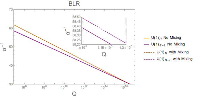
Figure 1: Comparison of RGE evolution with (solid lines) and without (dashed lines) gauge-kinetic mixing from GUT to SUSY scale. The $U(1)_{R}$ evolution is unchanged, whereas the $U(1)_{B-L}$ is modified slightly. A zoomed in plot of this modification is shown.

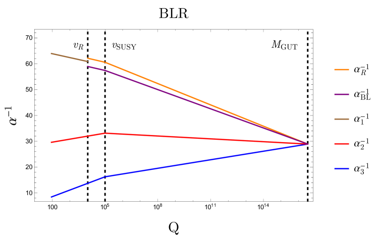
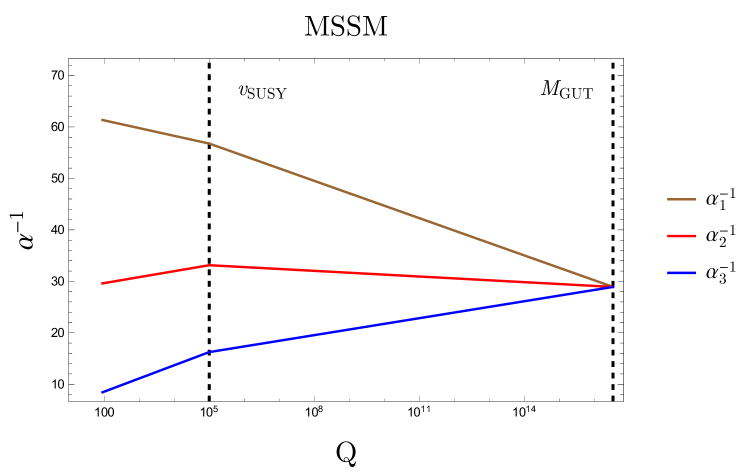
Figure 2: The upper panel shows the running couplings in the BLR model, with $v_{R}=11660$ GeV, which corresponds to $M_{Z^{\prime}}=3750$ GeV and $v_{\rm SUSY}=10^{5}$ GeV. The GUT scale is determined to be $M_{\rm GUT}=3.30\times 10^{16}$ GeV. The lower panel shows the running couplings in the MSSM.

We include GKM from the SUSY scale to the $U(1)_{R}\times U(1)_{B-L}$ breaking scale, $v_{R}$. From $v_{R}<Q<v_{\rm SUSY}$, decoupling the SUSY particles, the $\beta$-function coefficients change to $b_{BL}^{\rm BLR}=17/4$, $b_{R}^{\rm BLR}=13/3$ and a mixed term $b_{R,B-L}^{\rm BLR,SUSY}=b_{B-L,R}^{\rm BLR,SUSY}=-1/\sqrt{24}$. We summarise these beta function coefficients and their meaning in appendix B. At $v_{R}$ these two coupling values determine the (GUT normalised) hypercharge coupling,

$$\alpha^{-1}_{1} =\frac{3}{5}\alpha^{-1}_{R}+\frac{2}{5}\alpha_{BL}^{-1}.$$ (26)

From this scale, $\alpha_{1}$ is run further down from $v_{R}$ to $M_{Z}$, with the SM $\beta$-function coefficient $b_{1}^{\rm SM}=41/10$. The BLR breaking scale has been chosen such that the VEV and coupling values at this point correspond to a $Z^{\prime}$ with a statistical significance $\leq 2\sigma$, which is seen later to be 3750 GeV. Using this $Z^{\prime}$ mass, the $v_{R}$ VEV is determined from the formula Hirsch:2012kv in the limit $\tilde{g}=0$,

$$M^{2}_{Z^{\prime}}=\frac{1}{4}\left(\frac{3}{2}g_{B-L}^{2}+g_{R}^{2}\right)v_{R}^{2}+\frac{\frac{1}{4}g_{R}^{4}v^{2}}{(3/2)g_{B-L}^{2}+g_{R}^{2}}\approx\frac{1}{4}\left(\frac{3}{2}g_{B-L}^{2}+g_{R}^{2}\right)v_{R}^{2},$$ (27)

where $\sqrt{(3/2)}g_{B-L}=0.563$, as seen in Eq.16, and $M_{Z^{\prime}}=3750~{}\textrm{GeV}$ leads to $v_{R}=10328~{}\textrm{GeV}$.

The upper panel of Fig. 2 shows the running couplings of the BLR model, setting $v_{R}=10328$ GeV and $v_{\rm SUSY}=10^{5}$ GeV. Using our one-loop RGEs, we predict a value for the SM hypercharge coupling as $\alpha_{Y}(M_{Z})=\dfrac{3}{5}\alpha_{1}(M_{Z})=1/102.44$, which we may compare to the experimentally determined value of $\alpha_{Y}^{\rm exp}=\dfrac{\alpha_{EM}}{1-\sin^{2}\theta_{W}}=1/98.39$ Patrignani:2016xqp . The difference between the two values may be partly accounted for by our procedure of running up the best fit experimental values of $\alpha_{2}$ and $\alpha_{3}$ at $M_{Z}$ to determine $M_{\rm GUT}$ and $\alpha_{\rm GUT}$ at the point where they meet, then running all the gauge couplings from this point down to low energies. This procedure, though convenient for the BLR model where the hypercharge gauge coupling is not defined above $v_{R}$, does not take into account the experimental error in $\alpha_{3}^{\rm exp}$ in the prediction for $\alpha_{Y}^{\rm exp}$. Another source of error is the fact that we do not consider either two loop RGEs or threshold effects, both of which are beyond the scope of this paper. Using our one loop results, we determine the values of the couplings in Eq.16, which refer to the non-GUT normalised couplings.

For comparison, the lower panel of Fig. 2 shows the MSSM at one-loop running couplings, again assuming $v_{\rm SUSY}=10^{5}$ GeV. In this case the analogous procedure to that used in the BLR model yields a prediction for the SM hypercharge coupling of $\alpha_{Y}^{\rm MSSM}(M_{Z})=1/102.25$.

VI Results

VI.1 Preliminaries

In this section, we review the LHC results specific to the BLR model in Drell-Yan (DY) processes as well as in final states including Higgs bosons. We do so in two separate subsections to follow. In the case of DY studies, we also compare the BLR results to those of the $U(1)_{B-L}$ scenario. Throughout our analysis we assume the aforementioned heavy SUSY scale, thereby preventing decays of the $Z^{\prime}$ into sparticles. However, we consider the possibility that the 2HDM-like Higgs states of the BLR models are lighter than the $Z^{\prime}$, which may therefore decay into them via the couplings in Tab. 4. Further, notice that $Z^{\prime}$ decays into non-MSSM-like Higgs states can be heavily suppressed in comparison, in virtue of the fact that the additional CP-odd state not giving mass to the $Z^{\prime}$ can be made arbitrarily heavy (as previously explained), a setup which we assume here, so that we refrain from accounting for these decay patterns. Finally, recall that heavy neutrino decays are prevented here in the light of footnote 2 and that they have already been studied in, e.g., Khalil:2015naa (for the $B-L$ case), from where it is clear that they have little $Z^{\prime}$ diagnostic power. In contrast, we aim at making the point that the Higgs decays we study below can eventually be used for this purpose.

We use standard 2HDM notation, such that $h^{0}$ and $H^{0}$ are the CP-even Higgs mass states (with the lighter $h^{0}$ being the discovered SM-like one), $A^{0}$ the CP-odd one and $H^{\pm}$ the charged ones.

Tab. 5 summarises the numerical values of the vector and axial couplings of the $Z^{\prime}$ to fermions for the $B-L$ and BLR models. For each scenario we have defined new vector and axial couplings with the gauge coupling absorbed:

$$-\mathcal{L}^{Z^{\prime}}=Z_{\mu}^{\prime}\bar{f}\gamma^{\mu}\frac{1}{2}(\bar{g}^{f}_{V}-\bar{g}^{f}_{A}\gamma^{5})f,$$ (28)

which may be compared to Eq. 17. For the $U(1)_{B-L}$ model the calculation of $\bar{g}^{f}_{V,A}$ in Tab. 5 uses the gauge coupling constants shown there multiplied by the vector and axial couplings given previously in Tab. 3. For the BLR model, the new numerical vector and axial couplings are derived including the full effects of gauge-kinetic mixing using SARAH (as a function of the mixed couplings $g_{BL,R},~{}g_{R,BL}$ and the rotation matrix which diagonalises the neutral gauge boson mass matrices), but may be approximated analytically neglecting GKM using Eqs.14,17 as

$$\bar{g}^{f}_{V,A}({\rm BLR})\approx g_{Y}\left[(\cot\theta_{BL})g^{f}_{V,A}(R)-(\tan\theta_{BL})g^{f}_{V,A}(BL)\right]$$ (29)

in terms of the vector and axial couplings $g^{f}_{V,A}(R)$ and $g^{f}_{V,A}(BL)$ for the $T_{3R}$ and $T_{B-L}$ models as written in Tab. 3. The non-GUT normalised gauge couplings for the BLR model in Eq.29 and Tab. 5 come from the RGE analysis leading to Eq.16. The values of the non-GUT normalised gauge couplings $g_{BL}$ and $g_{\chi}$ for the $B-L$ and $\chi$ models in Tab. 5 were taken from the low energy parametrisation in Accomando:2010fz rather than an RGE analysis, which would require us to specify the corresponding high energy models, which we do not wish to do here, bearing in mind that the $B-L$ model does not emerge from $SO(10)$. If some other value of $g_{BL}$ were used instead, then the vector and axial couplings for the $B-L$ model in Tab. 5 would be straightforwardly rescaled.

Many qualitative features of the results can be understood by examining the fermion couplings in Tab. 5, for example, the vector nature of the $B-L$ couplings.

Model	Gauge Coupling	$\bar{g}_{V}^{u}$	$\bar{g}_{A}^{u}$	$\bar{g}_{V}^{d}$	$\bar{g}_{A}^{d}$	$\bar{g}_{V}^{e}$	$\bar{g}_{A}^{e}$	$\bar{g}_{V}^{\nu}$	$\bar{g}_{A}^{\nu}$
$B-L$	$g_{BL}$=0.592	0.197	0	0.197	0	-0.592	0	-0.296	-0.296
BLR	See Eq.16	-0.0103	-0.135	-0.279	0.135	0.300	0.135	0.217	0.217

Table 5: Numerical values of the vector and axial couplings for the $U(1)_{B-L}$ and $U(1)_{B-L}\times U(1)_{R}$ models. Note that we have decoupled the right-handed neutrinos in calculating $g_{V}^{\nu}$ and $g_{A}^{\nu}$.

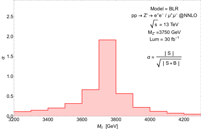
(a)

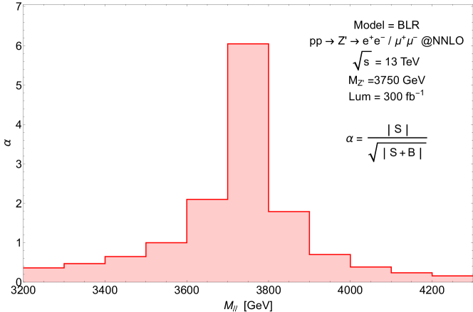
(b)

Figure 3: Statistical significance for producing a $Z^{\prime}$ decaying into $e^{+}e^{-}$ and $\mu^{+}\mu^{-}$ in the BLR model at integrated luminosities of (a) $L=30$ fb^-1 and (b) $300$ fb^-1. The number of events obtained at these luminosities for $pp\to Z^{\prime}$ is 74 in case (a) and 737 in case (b).

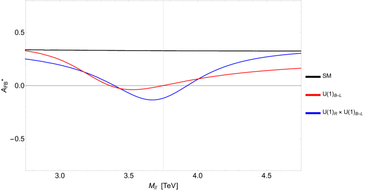
Figure 4: The theoretical predictions of the leptonic forward-backward asymmetry at the LHC $A^{*}_{\rm FB}$ in the presence of a $Z^{\prime}$ decaying into $e^{+}e^{-}$ and $\mu^{+}\mu^{-}$ for the $U(1)_{Y}\times U(1)_{B-L}$ (red) and $U(1)_{R}\times U(1)_{B-L}$ (blue) models. We have taken $M_{Z^{\prime}}=3750$ GeV. The SM (black) result is also given for comparison.

VI.2 Drell-Yan

The most promising channel to search for and profile a $Z^{\prime}$ boson at the LHC in the BLR model is DY production and decay, namely, $pp\to\gamma,Z,Z^{\prime}\to$ $e^{+}e^{-}$ and $\mu^{+}\mu^{-}$. Fig. 3a illustrates the current LHC reach (assuming 30 fb^-1 of integrated luminosity at 13 TeV), highlighting that a $Z^{\prime}$ of BLR origin with a mass of 3750 GeV is allowed by data, as its statistical significance $\alpha\equiv\frac{|S|}{\sqrt{|S+B}|}$ is less than 2 in the entire mass range over which the signal $|S|$ could manifest itself over the background $|B|$. Notice that, here and in the following, our signal is given by the (modulus of the) cross section of $pp\to\gamma,Z,Z^{\prime}\to$ $e^{+}e^{-}$ and $\mu^{+}\mu^{-}$ minus that of $pp\to\gamma,Z\to$ $e^{+}e^{-}$ and $\mu^{+}\mu^{-}$ (thereby including interference effects between $Z^{\prime}$ and $\gamma,Z$), the latter being the (irreducible) background. This very same $Z^{\prime}$ boson will, however, become accessible by the end of Run 2 of the LHC, as illustrated in Fig. 3b, where (assuming 300 fb^-1 of integrated luminosity at 13 TeV) values of $\alpha$ in excess of 5 are found near the peak region.

Once such a $Z^{\prime}$ signal is established, it will be necessary to diagnose it, i.e., to assess to which model it belongs. A useful variable in this respect is the (reconstructed) Forward-Backward Asymmetry ($A^{*}_{\rm FB}$) of the DY cross section. We use here the definition adopted in Ref. Accomando:2015cfa , see Sect. 3 therein, with no cut on the the di-lepton rapidity (see also Refs. Accomando:2015ava ; Accomando:2015pqa ). Fig. 4 shows the shape of this observable at the LHC, for $\sqrt{s}=13$ TeV and $M_{Z^{\prime}}=3750$ GeV, as it would appear in the $Z^{\prime}$ peak region of the di-lepton invariant mass distribution for the BLR model as well as the $U(1)_{B-L}$ scenario. The shape emerging from the BLR case is notably different from the one of the companion $SO(10)$ model.

In order to quantify whether the LHC will be able to differentiate these two models, from one another or the SM, one must include the statistical error in the formulation of $A^{*}_{\rm FB}$ Accomando:2015ava :

$$\delta A_{\rm FB}=\sqrt{\frac{1-A_{\rm FB}^{2}}{N}}.$$ (30)

In Fig. 5 we include this error in a binned version of Fig. 4, which overlays the $U(1)_{B-L}$ and BLR models, for a luminosity of 3000 fb^-1 corresponding to the final result for the High-Luminosity LHC (HL-LHC) run Gianotti:2002xx . The purple region is the overlap of errors between the two models. One can see that there are areas where the errors do not overlap and, by looking at the entire invariant mass distribution, a detailed statistical analysis may in principle differentiate between these two models at this luminosity, although we leave this task to the experimental collaborations.

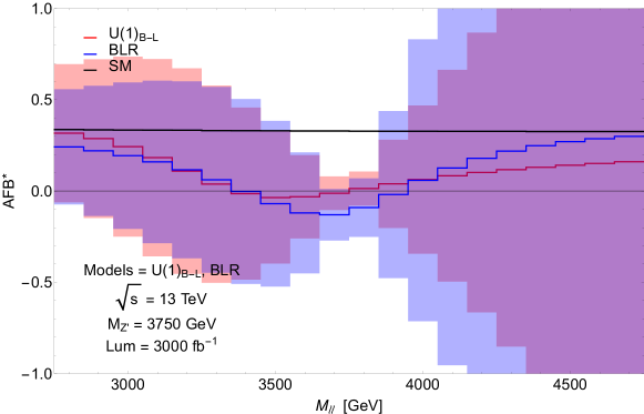
Figure 5: The $A^{*}_{\rm FB}$ spectrum of the DY cross section in the presence of a $Z^{\prime}$ of mass $M_{Z^{\prime}}=3750$ GeV. The figure we shows the BLR model prediction for $A_{\rm FB}^{*}$ (in blue) and its error (shaded in light blue) as well as the $U(1)_{B-L}$ prediction for $A_{\rm FB}^{*}$ (in red) and its error (shaded in light red) as a function of the dilepton invariant mass. The purple region is the overlap of errors between the two models. Here, $L=3000$ fb^-1.

VI.3 Higgs Final States

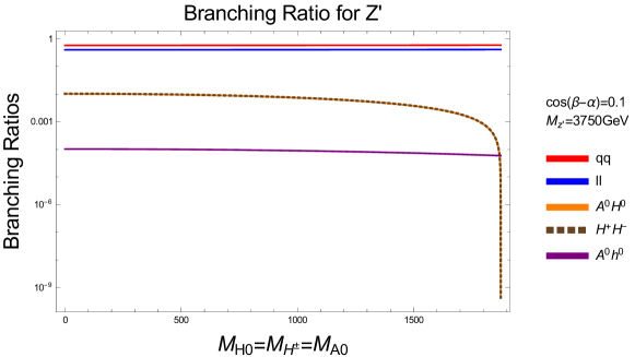
Figure 6: BRs of a $Z^{\prime}$ in the BLR model as a function of degenerate $A_{0}$, $H^{0}$ and $H^{\pm}$ masses. Here, $M_{Z^{\prime}}=3750$ GeV and $\cos(\beta-\alpha)=0.1$.

An alternative way of singling out the BLR nature of a $Z^{\prime}$ signal established via DY studies would the one pursuing the isolation of its exotic decays, i.e., into non-SM objects. Under the enforced assumption of heavy neutrinos, additional CP-odd Higgs boson and all sparticles being (much) heavier than the $Z^{\prime}$, the latter would include those into all possible MSSM-like (pseudo)scalar states pertaining to the Higgs sector of the BLR model, which, as discussed while commenting Tab. 1, is notably different from those of the $U(1)_{B-L}$ scenario. In particular, in presence of CP conservation, the following decay channels would be allowed in the BLR framework: $Z^{\prime}\to A^{0}h^{0}$, $A^{0}H^{0}$ and $H^{+}H^{-}$. These are presented for the usual $Z^{\prime}$ benchmark, assuming $\cos(\beta-\alpha)=0.1$ (so as to comply with LHC data from Higgs studies), in Fig. 6, for representative values of the Higgs boson masses. While the corresponding BRs are always subleading (of ${\cal O}(10^{-4})$ to ${\cal O}(10^{-2})$) with respect to those of the decays into SM fermions, the (on-shell) $Z^{\prime}$ cross section is 2.46 fb, so that HL-HLC luminosities should render the extraction of these decay modes possible, whichever the final decay patterns of the Higgs bosons involved.

VII Conclusion

$SO(10)$ GUTs have the remarkable property that they predict right-handed neutrinos, making neutrino mass inevitable. $SO(10)$ is also a rank 5 gauge group, which implies that any rank preserving GUT breaking sector will lead to an extra Abelian factor in the low energy effective theory, which protects right-handed neutrinos from gaining mass. If the rank is broken at the TeV scale, then there will be a $Z^{\prime}$ and massive right-handed neutrinos possibly observable at the LHC.

We have considered $SO(10)$ motivated $Z^{\prime}$ models. In particular we have focussed on the breaking pattern in Eq. 3, where the final breaking scale in Eq. 5, of the $U(1)_{R}\times U(1)_{B-L}$ Abelian subgroup into the hypercharge $U(1)_{Y}$ of the SM, may be around the TeV scale without spoiling gauge unification, within the accuracy of our one-loop analysis. The SUSY version of the $U(1)_{R}\times U(1)_{B-L}$  (BLR) model permits a linear seesaw mechanism for neutrino mass generation.

After defining the BLR model particle content and giving the relevant $Z^{\prime}_{BLR}$ and Higgs couplings, we have focussed on the discovery prospects of the $Z^{\prime}_{BLR}$ at the LHC, its decay into Higgs states, and the forward-backward asymmetry as a diagnostic for discriminating it from the $Z^{\prime}_{BL}$ of the $U(1)_{Y}\times U(1)_{B-L}$ model. It is noteworthy that the $Z^{\prime}_{BL}$ of the $B-L$ model has purely vector couplings to quarks and leptons, making the forward-backward asymmetry a powerful discriminator, as we have discussed. In general, we have set out to test whether such models can be disentangled at past (like LEP/SLC) and present (like LHC) machines, assuming that the SUSY scale is higher than the $Z^{\prime}_{BLR}$ mass.

Having determined the parameters of the BLR model to one-loop accuracy at the TeV scale, we have examined the feasibility of the LHC to extract a $Z^{\prime}_{BLR}$ signal. We have shown that $Z^{\prime}_{BLR}$ mass values just below the current sensitivity of the LHC can easily be accessed by the end of Run 2 in standard DY searches exploiting electron and muon final states. Furthermore, we have made a detailed investigation of $A^{*}_{\rm FB}$ (i.e., the reconstructed forward-backward asymmetry) of these di-lepton final states and shown that it may be possible to distinguish the $Z^{\prime}_{BLR}$ of the $U(1)_{R}\times U(1)_{B-L}$ from the $Z^{\prime}_{BL}$ of the $U(1)_{Y}\times U(1)_{B-L}$ case, assuming HL-LHC luminosities. This is probably the main new result of this paper.

We have also considered the $Z^{\prime}_{BLR}$ decays into MSSM-like Higgs bosons, which would include $Z^{\prime}_{BLR}\to A^{0}h^{0}$, $A^{0}H^{0}$ and $H^{+}H^{-}$, but excluding possible decays into $\chi_{R}^{1}$ and $\chi_{R}^{2}$ bosons which we assume to be too heavy to be produced. While the Higgs decay rates are always small, from percent to fraction of permille level, compared to those into SM leptons and quarks, HL-HLC luminosities should render the extraction of all of these signals feasible. Though such decays are often neglected in the literature, they provide an additional Higgs production mechanism, possibly the dominant mechanism on the $Z^{\prime}_{BLR}$ resonance at an $e^{+}e^{-}$ collider, and a crucial test of the gauge structure of the model in the 2HDM versions of the models that SUSY demands.

Appendix A Linear Seesaw

The linear seesaw is similar to an inverse seesaw, but with $\mu\rightarrow 0$ and a new term coupling a left-handed (LH) neutrino to the scalar singlet $S$:

$$\begin{pmatrix}0&Yv&Fv_{L}\\ Y^{T}v&0&\tilde{F}v_{R}\\ F^{T}v_{L}&\tilde{F}^{T}v_{R}&0\end{pmatrix}\equiv\begin{pmatrix}0&m_{D}&\epsilon\\ m_{D}^{T}&0&M_{\chi}\\ \epsilon^{T}&M_{\chi}^{T}&0\end{pmatrix}.$$ (31)

Each element here corresponds to a $3\times 3$ block. Solving this in block diagonal form, assuming $\epsilon\ll m_{D}\ll M_{\chi}$, one finds

$$\begin{pmatrix}M_{\chi}+m_{D}^{T}m_{D}M_{\chi}^{-1}&0&0\\ 0&-(M_{\chi}+m_{D}^{T}m_{D}M_{\chi}^{-1})&0\\ 0&0&-\epsilon\frac{m_{D}^{T}}{M_{\chi}}\end{pmatrix}.$$ (32)

So the light and heavy physical masses are

$$M_{\nu_{L}} =-\epsilon\frac{m_{D}^{T}}{M_{\chi}}+\textrm{h.c.}$$ (33)

$$M_{N_{1}}\sim M_{N_{2}} \sim M_{\chi}+m_{D}^{T}m_{D}M_{\chi}^{-1}+\textrm{h.c.}$$ (34)

Here we have the light neutrinos, $\nu_{L}$, as observed in oscillation experiments, and $N_{1,2}$ are the heavier neutral fermions. The smallness of $\epsilon$ may allow for a low (TeV) scale $M_{\chi}$, which is a fundamental feature of all low-scale seesaw mechanisms. Unlike the inverse seesaw, we see that $M_{\nu_{l}}$ is linear in $m_{D}$, which is proportional to the Yukawa couplings, hence the name “linear” seesaw.

Appendix B RGEs

$\left.\begin{tabular}[]{c | c | c | c}\hskip 11.38092pt \phantom{$b_{R,B-L}^{BLR}=b_{B-L,R}^{BLR}$}&\phantom{GUT normalisation}&\phantom{$-1/\sqrt{24}$}&\phantom{$M_{\mathrm{SUSY}}<Q<M_{\mathrm{\rm GUT}}$}\\[-12.0pt] Coefficient&GUT normalisation&Value&Scale\vspace{-0.065cm}\end{tabular}\color[rgb]{1,1,1}\right\}$Non-Abelian $\left.\begin{tabular}[]{c | c | c | c}\phantom{Coefficient}&\phantom{GUT normalisation}&\phantom{Value}&\phantom{Scale}\\[-12.0pt] \hline\cr\hbox{\multirowsetup$b_{R,R}^{BLR}$}&\hbox{\multirowsetup 1}&15/2&$M_{\mathrm{SUSY}}<Q<M_{\mathrm{\rm GUT}}$\\ &&13/3&$M_{\mathrm{BLR}}<Q<M_{\mathrm{SUSY}}$\\ \hline\cr\hbox{\multirowsetup$b_{(B-L),(B-L)}^{BLR}$}&\hbox{\multirowsetup$3/8$}&27/4&$M_{\mathrm{SUSY}}<Q<M_{\mathrm{\rm GUT}}$\\ &&17/4&$M_{\mathrm{BLR}}<Q<M_{\mathrm{SUSY}}$\\ \hline\cr\hbox{\multirowsetup$b_{R,B-L}^{BLR}=b_{B-L,R}^{BLR}$}&\hbox{\multirowsetup$\sqrt{3/8}$}&$-\sqrt{3/8}$&$M_{\mathrm{SUSY}}<Q<M_{\mathrm{\rm GUT}}$\\ &&$-1/\sqrt{24}$&$M_{\mathrm{BLR}}<Q<M_{\mathrm{SUSY}}$\vspace{-0.065cm}\\ \end{tabular}\right\}$ Abelian $\left.\hskip 21.33955pt\begin{tabular}[]{c | c | c | c}\phantom{$b_{R,B-L}^{BLR}=b_{B-L,R}^{BLR}$}&\phantom{GUT normalisation}&\phantom{$-1/\sqrt{24}$}&\phantom{Scale}\\[-12.0pt] \hline\cr\hbox{\multirowsetup$B_{3}^{BLR}$}&1&-3&$M_{\mathrm{SUSY}}<Q<M_{\mathrm{\rm GUT}}$\\ &1&-7&$M_{\mathrm{BLR}}<Q<M_{\mathrm{SUSY}}$\\ &1&-7&$M_{\mathrm{EW}}<Q<M_{\mathrm{BLR}}$\\ \hline\cr\hbox{\multirowsetup$B_{2}^{BLR}$}&1&1&$M_{\mathrm{SUSY}}<Q<M_{\mathrm{\rm GUT}}$\\ &1&-19/6&$M_{\mathrm{BLR}}<Q<M_{\mathrm{SUSY}}$\\ &1&-19/6&$M_{\mathrm{EW}}<Q<M_{\mathrm{BLR}}$\\ \end{tabular}\right\}$Non-Abelian

Table 6: Beta function coefficients for Abelian and non-Abelian gauge groups in the BLR model

Beta functions for the non-Abelian and Abelian groups, respectively, are Bertolini:2009qj

$$\frac{\textrm{d}g_{a}}{\textrm{d}t}=\frac{B_{a}g_{a}^{3}}{16\pi^{2}}~{},~{}~{}\frac{dg_{lm}}{dt}=\frac{g_{lk}}{16\pi^{2}}b_{ij}g_{ik}g_{jm},$$ (35)

where the index $a$ runs over the non-Abelian groups $SU(2)_{L}$ and $SU(3)_{c}$, $a=2,3$ and $(i,j,k,l,m)$ run over the $U(1)_{R},~{}U(1)_{B-L}$, and mixed $U(1)_{R}\times U(1)_{B-L}$ and $U(1)_{B-L}\times U(1)_{R}$ groups, $(i,j,k,l,m)=(R,B-L)$ and Einstein summation convention is assumed. For our RGE section, we make a rotation on the coupling matrix $G$, such that it is set in upper triangular form Coriano:2015sea

$$G=\begin{pmatrix}g_{11}&g_{12}\\ g_{21}&g_{22}\end{pmatrix}$$ (36)

$$\tilde{G}=GO^{T}_{R}=\begin{pmatrix}g&\tilde{g}\\ 0&g^{\prime}\end{pmatrix}=\left(\begin{array}[]{cc}\frac{g_{11}g_{22}-g_{12}g_{21}}{\sqrt{g_{21}^{2}+g_{22}^{2}}}&\frac{g_{11}g_{21}+g_{12}g_{22}}{\sqrt{g_{21}^{2}+g_{22}^{2}}}\\ 0&\sqrt{g_{21}^{2}+g_{22}^{2}}\\ \end{array}\right)$$ (37)

One may consequently find the RGE in terms of $g,~{}g^{\prime},~{}\tilde{g}$ by differentiating these expressions and then replacing the differentials $dg_{ij}/dt$ with the beta functions as calculated with eq. 35, then replacing $g_{11},g_{12},g_{22}$ in terms of $g,~{}g^{\prime},~{}\tilde{g}$.

References

- (1) S. F. King, JHEP 1708 (2017) 019 [arXiv:1706.06100 [hep-ph]]; B. S. Acharya, K. Bozek, M. Crispim Romao, S. F. King and C. Pongkitivanichkul, JHEP 1611 (2016) 173 [arXiv:1607.06741 [hep-ph]].
- (2) S. F. King and T. Yanagida, Prog. Theor. Phys. 114 (2006) 1035 [hep-ph/0411030].
- (3) S. Khalil and A. Masiero, Phys. Lett. B 665 (2008) 374 doi:10.1016/j.physletb.2008.06.063 [arXiv:0710.3525 [hep-ph]].
- (4) P. Fileviez Perez and S. Spinner, Phys. Rev. D 83 (2011) 035004 doi:10.1103/PhysRevD.83.035004 [arXiv:1005.4930 [hep-ph]].
- (5) B. O’Leary, W. Porod and F. Staub, JHEP 1205 (2012) 042 doi:10.1007/JHEP05(2012)042 [arXiv:1112.4600 [hep-ph]].
- (6) A. Elsayed, S. Khalil and S. Moretti, Phys. Lett. B 715 (2012) 208 doi:10.1016/j.physletb.2012.07.066 [arXiv:1106.2130 [hep-ph]].
- (7) G. Arcadi, M. Lindner, Y. Mambrini, M. Pierre and F. S. Queiroz, Phys. Lett. B 771 (2017) 508 doi:10.1016/j.physletb.2017.05.023 [arXiv:1704.02328 [hep-ph]].
- (8) E. Accomando, A. Belyaev, L. Fedeli, S. F. King and C. Shepherd-Themistocleous, Phys. Rev. D 83 (2011) 075012 doi:10.1103/PhysRevD.83.075012 [arXiv:1010.6058 [hep-ph]].
- (9) P. Langacker, Rev. Mod. Phys. 81 (2009) 1199 [arXiv:0801.1345 [hep-ph]].
- (10) M. Malinsky, J. C. Romao and J. W. F. Valle, Phys. Rev. Lett. 95 (2005) 161801 [hep-ph/0506296].
- (11) M. Hirsch, S. Morisi and J. W. F. Valle, Phys. Lett. B 679 (2009) 454 [arXiv:0905.3056 [hep-ph]].
- (12) V. De Romeri, M. Hirsch and M. Malinsky, Phys. Rev. D 84 (2011) 053012 [arXiv:1107.3412 [hep-ph]].
- (13) M. Hirsch, M. Malinsky, W. Porod, L. Reichert and F. Staub, JHEP 1202 (2012) 084 [arXiv:1110.3037 [hep-ph]].
- (14) M. Hirsch, W. Porod, L. Reichert and F. Staub, Phys. Rev. D 86 (2012) 093018 [arXiv:1206.3516 [hep-ph]].
- (15) L. Basso et al., Comput. Phys. Commun. 184 (2013) 698 [arXiv:1206.4563 [hep-ph]].
- (16) M. Frank and O. Ozdal, arXiv:1709.04012 [hep-ph].
- (17) J. Chakrabortty and A. Raychaudhuri, Phys. Rev. D 81 (2010) 055004 doi:10.1103/PhysRevD.81.055004 [arXiv:0909.3905 [hep-ph]]; arXiv:1711.11391 [hep-ph].
- (18) M. E. Krauss, W. Porod and F. Staub, Phys. Rev. D 88 (2013) no.1, 015014 doi:10.1103/PhysRevD.88.015014 [arXiv:1304.0769 [hep-ph]].
- (19) F. Staub, Comput. Phys. Commun. 185 (2014) 1773 doi:10.1016/j.cpc.2014.02.018 [arXiv:1309.7223 [hep-ph]].
- (20) C. Coriano, L. Delle Rose and C. Marzo, JHEP 1602 (2016) 135 doi:10.1007/JHEP02(2016)135 [arXiv:1510.02379 [hep-ph]].
- (21) S. Bertolini, L. Di Luzio and M. Malinsky, Phys. Rev. D 80 (2009) 015013 doi:10.1103/PhysRevD.80.015013 [arXiv:0903.4049 [hep-ph]].
- (22) C. Patrignani et al. [Particle Data Group], Chin. Phys. C 40 (2016) no.10, 100001.
- (23) W. Abdallah, J. Fiaschi, S. Khalil and S. Moretti, Phys. Rev. D 92 (2015) 055029 [arXiv:1504.01761 [hep-ph]].
- (24) W. Abdallah, J. Fiaschi, S. Khalil and S. Moretti, JHEP 1602 (2016) 157 [arXiv:1510.06475 [hep-ph]].
- (25) M. Aaboud et al. [ATLAS Collaboration], Phys. Lett. B 761 (2016) 372 doi:10.1016/j.physletb.2016.08.055 [arXiv:1607.03669 [hep-ex]].
- (26) V. Khachatryan et al. [CMS Collaboration], Phys. Lett. B 768 (2017) 57 doi:10.1016/j.physletb.2017.02.010 [arXiv:1609.05391 [hep-ex]].
- (27) E. Accomando, A. Belyaev, J. Fiaschi, K. Mimasu, S. Moretti and C. Shepherd-Themistocleous, JHEP 1601 (2016) 127 [arXiv:1503.02672 [hep-ph]]; E. Accomando, D. Becciolini, A. Belyaev, S. Moretti and C. Shepherd-Themistocleous, JHEP 1310 (2013) 153 doi:10.1007/JHEP10(2013)153 [arXiv:1304.6700 [hep-ph]].
- (28) E. Accomando, A. Belyaev, J. Fiaschi, K. Mimasu, S. Moretti and C. Shepherd-Themistocleous, Nuovo Cim. C 38 (2016) no.4, 153 [arXiv:1504.03168 [hep-ph]].
- (29) J. Fiaschi, E. Accomando, A. Belyaev, K. Mimasu, S. Moretti and C. H. Shepherd-Themistocleous, PoS EPS -HEP2015 (2015) 176 [arXiv:1510.05892 [hep-ph]].
- (30) F. Gianotti et al., Eur. Phys. J. C 39 (2005) 293 [hep-ph/0204087].
- (31) S. Khalil and S. Moretti, Rept. Prog. Phys. 80 (2017) no.3, 036201 [arXiv:1503.08162 [hep-ph]].