Finite-time and exact Lyapunov dimension of the Henon map.
Abstract
This work is devoted to further consideration of the Hénon map with negative values of the shrinking parameter and the study of transient oscillations, multistability, and possible existence of hidden attractors. The computation of the finite-time Lyapunov exponents by different algorithms is discussed. A new adaptive algorithm for the finite-time Lyapunov dimension computation in studying the dynamics of dimension is used. Analytical estimates of the Lyapunov dimension using the localization of attractors are given. A proof of the conjecture on the Lyapunov dimension of self-excited attractors and derivation of the exact Lyapunov dimension formula are revisited.
I Introduction
In 1963, American mathematician and meteorologist Edward Lorenz published an article in which he investigated an approximate model of the fluid convection in a two-dimensional layer and discovered its irregular behavior Lorenz-1963 . The analysis of this behavior was closely related to the phenomenon of chaos, namely to the sensitive dependence on the initial conditions and the existence in the phase space of the system of a chaotic attractor with a complex geometrical structure. Later, this three-dimensional system was called the Lorenz system, and so far it has great scientific interest Tucker-1999 ; Stewart-2000 ; LeonovK-2015-AMC .
In 1969, French mathematician and astronomer, Michel Hénon, showed that the essential properties of the Lorenz system (i.e., folding and shrinking of volumes) can be preserved by means of a specially chosen sequence of approximating maps Henon-1976 . The Poincaré map of the Lorenz system was chosen as the reference, resulting in the following map , where
| (1) |
(folding parameter), and (shrinking parameter) are parameters of mapping. One usually considers an equivalent form of the Hénon map (e.g. BoichenkoL-2000 ; Hunt-1996 ; GrassbergerKM-1989 )
| (2) |
obtained from (1) by changing the coordinates , . Along with positive values of parameter , considered in Henon-1976 , later on one also studies the Hénon system with negative values Feit-1978 ; Heagy-1992 .
The Hénon map and its various generalizations have attracted the attention of researchers with its comparative simplicity and the ability to model its dynamics without integrating differential equations (see, e.g. BenedicksC-1991 ; BenedicksY-1993 ; GrassbergerKM-1989 ; SterlingDM-1999 ; GonchenkoGS-2010 ; FalcoliniTL-2013 ; GaliasT-2013 ). Despite being introduced initially as a theoretical transformation, it also has several physical interpretations BihamW-1989 ; Heagy-1992 . Further, we will study Hénon map in the form (2) with , .
II Transient oscillations, attractors and multistability
Consider a dynamical system with discrete time generated by the recurrence equation with map (2)
| (3) |
where , , and with .
The equilibria of the system (3) exist when . Here
The Jacobian matrix is defined as follows:
| (4) |
where , and has the eigenvalues , and eigenvectors . One can check that equilibrium is always unstable and is unstable when .
In the seminal work Henon-1976 for a fixed value it was shown numerically that for and any trajectory tends to infinity for all . For , depending on the initial point , the trajectory either tends to infinity, or reaches the attractor that is a stable equilibrium for , a periodic orbit for , and a nontrivial chaotic attractor for . These numerical experiments imply that there is no global attractor in the Hénon system for .
Computational errors (caused by finite precision arithmetic) and sensitivity to initial conditions allow one to get a reliable visualization of chaotic attractor by only one pseudo-trajectory computed for a sufficiently large time interval.
Definition 1 (KuznetsovLV-2010-IFAC ; LeonovKV-2011-PLA ; LeonovKV-2012-PhysD ; LeonovK-2013-IJBC )
An attractor is called a self-excited attractor if its basin of attraction intersects with any open neighborhood of a stationary state (an equilibrium), otherwise, it is called a hidden attractor.
For a self-excited attractor its basin of attraction is connected with an unstable equilibrium and, therefore, self-excited attractors can be localized numerically by the standard computational procedure in which after a transient process a trajectory, started in a neighborhood of an unstable equilibrium (e.g., from a point of its unstable manifold), is attracted to the state of oscillation and then traces it. Thus, self-excited attractors can be easily visualized (e.g. the classical Lorenz and Rössler attractors can be visualized by a trajectory from a vicinity of unstable zero equilibrium).
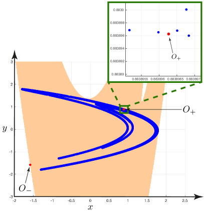
For , the equilibria are saddles (, ) and one can visualize the classical Hénon attractor Henon-1976 (see Fig. 1) from the -vicinity of using trajectories with the initial data
Similar self-excited attractor can be also obtained for negative values of parameter (e.g. for , in Feit-1978 ; Heagy-1992 ).
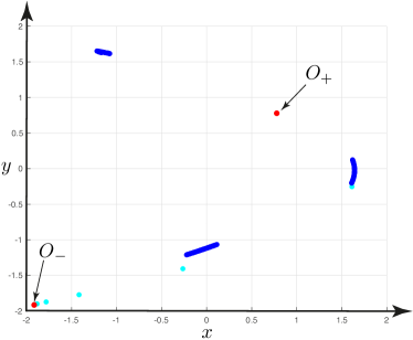
In DudkowskiPK-2016 the multistability and possible existence of hidden attractor in the Hénon system , were studied by the perpetual point method Prasad-2015 ; DudkowskiJKKLP-2016 . For these values of parameters , and from the initial point
on the unstable manifold of the saddle , defined by the eigenvector , a chaotic attractor in Fig. 2a can be visualized. Thus, the chaotic attractor obtained in DudkowskiPK-2016 is a self-excited attractor with respect to . In addition, a self-excited periodic attractor can be visualized from vicinity of . See coexisting self-excited periodic and chaotic attractors and their basins of attraction in Fig. 2b.
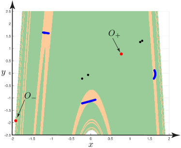
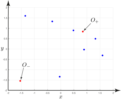
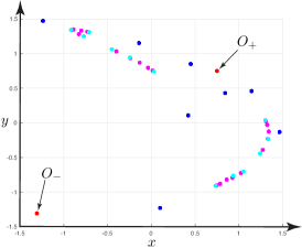
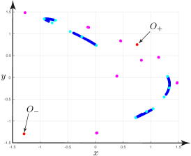
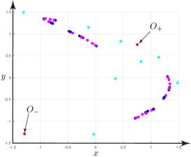
In GaliasT-2013 the multistability in the Hénon system was studied for positive parameters. In Fig. 4a, for parameters , there are three co-existing self-excited attractors: period-8 orbit self-excited with respect to (used initial data , ), period-12 orbit self-excited with respect to (used initial data , ), and period-20 orbit self-excited with respect to (used initial data , ). In Fig. 4b, for parameters , there are three co-existing attractors: period-12 orbit self-excited with respect to (used initial data , ), period-16 orbit self-excited with respect to (used initial data , ), and chaotic attractor self-excited with respect to (used initial data , ). Last but no least, in Fig. 4c, for parameters , there are three co-existing self-excited attractors: period-8 orbit self-excited with respect to (used initial data , ), and two chaotic attractors each one self-excited with respect to (used initial data , , and , , respectively). In FalcoliniTL-2013 ; FalcoliniTL-2016 the coexistence of periodic orbits is studied near the critical cases when and the map becomes less and less dissipative. The possible existence of hidden chaotic attractors in the Hénon map requires further investigation.
In the numerical computation of trajectory over a finite-time interval it is often difficult to distinguish a sustained oscillation from a transient oscillation (a transient set in the phase space, e.g. chaotic or quasi periodic, which can nevertheless persist for a long time) GrebogiOY-1983 ; LaiT-2011 . Thus, a similar to the above classification can be introduced for the transient sets.
Definition 2 (DancaK-2017-CSF ; ChenKLM-2017-IJBC )
A transient oscillating set is called hidden if it does not involve and attract trajectories from a small neighborhood of equilibria; otherwise, it is called self-excited.
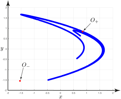
In the Hénon system (3) it is possible to observe the long-lived transient chaotic sets for and . For example, for it is possible to localize a self-excited transient chaotic set111 Similar behavior with hidden transient chaotic set can be obtained in various Lorenz-like systems, e.g. in the classical Lorenz system ChenKLM-2017-IJBC , in the Rabinovich system KuznetsovLMPS-2017-arXiv with respect to the saddle (, ) using the initial data
which persists for iterations and after that contracts into a period limit cycle.
In order to distinguish an attracting chaotic set (attractor) from a transient chaotic set in numerical experiments, one can consider a grid of points in a small neighborhood of the set and check the attraction of corresponding trajectories towards the set. Various examples of hidden transient chaotic sets localization are discussed, e.g., in DangLBW-2015-HA ; Danca-2016-HA ; YuanYW-2017-HA ; DancaK-2017-CSF ; ChenKLM-2017-IJBC .
In Feit-1978 , for parameters and , it is suggested an analytical bounded localization of attractors in the Hénon map by the set , where
| (5) | ||||
A similar set can be considered for negative values of .
Further by we denote a bounded closed invariant set, e.g. a maximum attractor with respect to the set of all nondivergent points from (i.e. ).
III Finite-time Lyapunov dimension and algorithms for its computation
The concept of the Lyapunov dimension was suggested in the seminal paper by Kaplan & Yorke KaplanY-1979 and later it has been developed and rigorously justified in a number of papers. Nowadays, various approaches to the Lyapunov dimension definition are used (see, e.g. Ledrappier-1981 ; EdenFT-1991 ). Below we consider the concept of the finite-time Lyapunov dimension Kuznetsov-2016-PLA ; KuznetsovLMPS-2017-arXiv , which is convenient for carrying out numerical experiments with finite time.
Let a nonempty closed bounded set be invariant with respect to dynamical system generated by (3) , i.e. for all (e.g. is an attractor). Further we use compact notations for the finite-time local Lyapunov dimension: , the finite-time Lyapunov dimension: , and for the Lyapunov dimension: .
Consider linearization of system (3) along the solution , :
| (6) |
Consider a fundamental matrix of solutions of linearized system (6) such that , i.e.
Then for any solution of (6) with the initial data we have
| (7) |
Let , be the singular values of (i.e. and are the eigenvalues of the symmetric matrix with respect to their algebraic multiplicity), ordered so that for any and . Consider the ordered set of the finite-time Lyapunov exponents at the point for :
| (8) |
Consider the Kaplan-Yorke formula KaplanY-1979 with respect to the ordered set :
| (9) |
For the ordered set of finite-time Lyapunov exponents and we get
Then for a certain point and invariant closed bounded set the finite-time local Lyapunov dimension Kuznetsov-2016-PLA ; KuznetsovLMPS-2017-arXiv is defined as
and the finite-time Lyapunov dimension is as follows
| (10) |
In this approach the use of Kaplan-Yorke formula (9) with the finite-time Lyapunov exponents can be rigorously justified by the Douady–Oesterlé theorem DouadyO-1980 , which implies that for any fixed the Lyapunov dimension of the map with respect to a closed bounded invariant set , defined by (10), is an upper estimate of the Hausdorff dimension of the set :
III.1 Adaptive algorithm for the computation of the finite-time Lyapunov dimension
To compute the finite-time Lyapunov exponents (8) one has to find the fundamental matrix of (6) from the following variational equation
| (11) | ||||
and its Singular Value Decomposition (SVD)
where , is a diagonal matrix composed by the singular values of , and compute the finite-time Lyapunov exponents from as in (8).
To avoid the exponential growth of values in the computation, we use the QR factorization and treppeniteration routine:
Then matrix can be approximated by sequential QR decomposition of the product of matrices:
where , , and RutishauserS-1963 ; Stewart-1997
For a large the convergence can be very rapid (Stewart-1997, , p. 44) (e.g. is taken in (Stewart-1997, , p. 44) for the Lorenz system with the classical parameters).
For the study of dynamics of the finite-time Lyapunov exponents KuznetsovLMPS-2017-arXiv we can adaptively choose for so as to obtain a uniform estimate with respect to :
| (12) |
Thus, the finite-time Lyapunov exponents can be approximated222 In Benettin’s algorithm BenettinGGS-1980-Part2 the so-called finite-time Lyapunov characteristic exponents (LCEs) Lyapunov-1892 , which are the exponential growth rates of norms of the fundamental matrix columns : are computed by (13) with : The following artificial analytical example demonstrates possible differences between LEs and LCEs: the matrix Kuznetsov-2016-PLA ; KuznetsovAL-2016 ; KuznetsovLMPS-2017-arXiv has , The approximation by Benettin’s algorithm becomes worse with increasing time: Remark that the notions of LCEs and LEs often do not differ (see, e.g. Eckmann & Ruelle (EckmannR-1985, , p.620,p.650), Wolf et al. (WolfSSV-1985, , p.286,p.290-291), and Abarbanel et al. (AbarbanelBST-1993, , p.1363,p.1364)), e.g. relying on ergodicity, however, the computations of LCEs by (13) and LEs by may give non relevant results. as
| (13) |
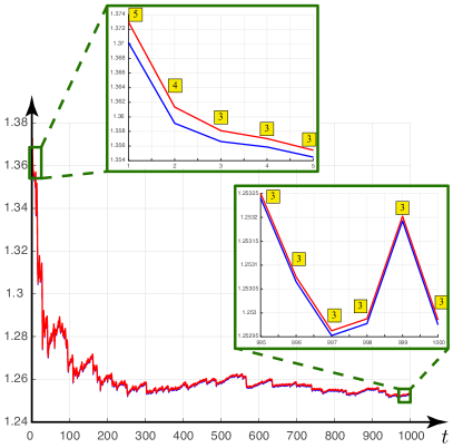
For the Hénon system (3) with canonical parameters , , using the described above adaptive algorithm with , we calculate the finite-time local Lyapunov dimension , where is the initial point of the trajectory that localizes the self-excited attractor (see Fig. 1). The comparison of the graphics for the adaptive algorithm and the algorithm with is presented in Fig. 6. For we obtain . The corresponding numerical routine implemented in MATLAB is presented in Appendix VI.
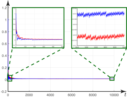
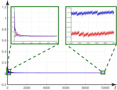
Applying the statistical physics approach and assuming the ergodicity (see, e.g. KaplanY-1979 ; Ledrappier-1981 ; FredericksonKYY-1983 ), the Lyapunov dimension of attractor is often estimated by the local Lyapunov dimension , corresponding to a “typical” trajectory, which belongs to the attractor: , and its limit value . However, rigorous check of ergodicity for the Henon system with a particular value of the parameters is a challenging task (see, e.g. BenedicksC-1991 ; BenedicksY-1993 ). See, also related discussions in BarreiraS-2000 (ChaosBook, , p.118)OttY-2008 (Young-2013, , p.9) (PikovskyP-2016, , p.19), and the works KuznetsovL-2005 ; LeonovK-2007 on the Perron effects of the largest Lyapunov exponent sign reversals. For example, consider parameters , (see Fig. 4c). In this case for , and , after a transient process during we get initial points and , respectively and compute finite-time Lyapunov exponents and finite-time local Lyapunov dimension for the time interval by the adaptive algorithm with : dynamics of the finite-time Lyapunov exponents and finite-time local Lyapunov dimension is presented in Fig. 5, finally we have
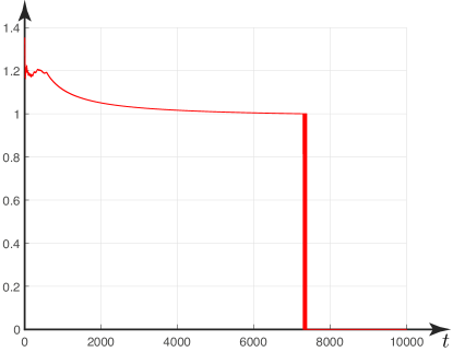
In one of the pioneering works by Yorke et al. (FredericksonKYY-1983, , p.190) the exact limit values of finite-time Lyapunov exponents, if they exist and are the same for all , are called the absolute ones, and it is noted that the absolute Lyapunov exponents rarely exist. Remark that while the time series obtained from a physical experiment are assumed to be reliable on the whole considered time interval, the time series, obtained numerically from mathematical dynamical model, can be reliable on a limited time interval only due to computational errors. Also, if the trajectory belongs to a transient chaotic set (see, e.g. Fig. 3), which can be (almost) indistinguishable numerically from sustained chaos, then any very long-time computation may be insufficient to reveal the limit values of the finite-time Lyapunov exponents and finite-time Lyapunov dimension (see Fig. 7)KuznetsovLMPS-2017-arXiv .
Thus, to get a reliable numerical estimation of the Lyapunov dimension of attractor we localize the attractor , consider a grid of points on , and find the maximum of the corresponding finite-time local Lyapunov dimensions for a certain time interval :
| (14) | |||
Additionally, we can consider a set of random points in , where is the number points in . If the maximum of the finite-time local Lyapunov dimensions for and are different, i.e. , then we decrease . This may help to improve reliability of the result and at the same time to ensure its repeatability.
IV The Lyapunov dimension: analytical estimations and exact value
To estimate the Hausdorff dimension of invariant closed bounded set , one can use the map with any time (e.g., leads to the trivial estimate ), and, thus, the best estimation is
The following property:
| (15) |
allows one to introduce the Lyapunov dimension of as Kuznetsov-2016-PLA
| (16) |
and get an upper estimation of the Hausdorff dimension:
Recall that a set with noninterger Hausdorff dimension is referred as a fractal set EckmannR-1985 .
In contrast to the finite-time Lyapunov dimension (10),
the Lyapunov dimension (16)333
This definition can be reformulated via the singular value function
where and is the largest integer less or equal to :
and .
Another approach to the introduction of the Lyapunov dimension of dynamical system
was developed by Constantin, Eden, Foiaş, and Temam
ConstantinFT-1985 ; Eden-1990 ; EdenFT-1991 .
They consider
instead of
and apply the theory of positive operators
to prove the existence of a critical point
(which may be not unique),
where the corresponding global Lyapunov dimension
achieves maximum (see Eden-1990 ):
and, thus, rigorously justify the usage of the local Lyapunov dimension
.
However this definition does not have a clear sense
for finite time.
is invariant under smooth change of coordinates KuznetsovAL-2016 ; Kuznetsov-2016-PLA .
This property and a proper choice of smooth change of coordinates
may significantly simplify the computation of the Lyapunov dimension of dynamical system.
Consider an effective analytical approach, proposed by Leonov Leonov-1991-Vest ; LeonovB-1992 ; Kuznetsov-2016-PLA ,
for estimating the Lyapunov dimension. In the work Kuznetsov-2016-PLA it is shown how this approach can be justified
by the invariance of the Lyapunov dimension of compact invariant set
with respect to the special smooth change of variables
with , where
is a continuous scalar function
and is a nonsingular matrix.
Let ,
be the singular values of
(i.e. the square roots of the eigenvalues of the symmetrized Jacobian matrix
),
ordered so that
for any .
Theorem 1 (Kuznetsov-2016-PLA )
If there exist a real , a continuous scalar function , and a nonsingular matrix such that
| (17) |
then
To avoid numerical localization of attractor, we can consider estimation (17) e.g. by the absorbing set or the whole phase space.
In BoichenkoL-1998 ; PogromskyM-2011 it is demonstrated how a technique similar to the above can be effectively used to derive constructive upper bounds of the topological entropy of dynamical systems.
If we consider and , then we get the Kaplan-Yorke formula with respect to the ordered set of logarithms of the singular values of the Jacobian matrix: and its supremum on the set gives an upper estimation of the finite-time Lyapunov dimension. This is a generalization of ideas, discussed e.g. in DouadyO-1980 ; Smith-1986 , on the Hausdorff dimension estimation by the eigenvalues of symmetrized Jacobian matrix.
The Jacobian (4) of the Hénon map (2) has the following singular values:
These expressions give the following estimation:
The maximum of the right-hand side value is determined by the maximum value of (or ) on . In Hunt-1996 , for canonical parameters , it was considered the square that gives the estimation
Using Feit’s analytical localization (5) we can get
For parameters , we obtain .
Remark, that if the Jacobian matrix at one of the equilibria has simple real eigenvalues: , then the invariance of the Lyapunov dimension with respect to linear change of variables implies Kuznetsov-2016-PLA the following
| (18) |
If the maximum of local Lyapunov dimensions on the B-attractor, involving all equilibria, is achieved at equilibrium point: , then this allows one to get analytical formula of the exact Lyapunov dimension444 This term was suggested by Doering et al. in DoeringGHN-1987 .. In general, a conjecture on the Lyapunov dimension of self-excited attractor Kuznetsov-2016-PLA ; KuznetsovL-2016-ArXiv is that the Lyapunov dimension of typical self-excited attractor does not exceed the Lyapunov dimension of one of unstable equilibria, the unstable manifold of which intersects with the basin of attraction and visualize the attractor.
Following Leonov-2002 for the Hénon system (3) with parameters and we can consider
In this case we have
and
If we take , then condition (17) with and
is satisfied for all and we do not need any localization of the set in the phase space. By (18) and (9), at the equilibrium point we get
Therefore, for a bounded invariant set (e.g. maximum B-attractor) we have Leonov-2002
Here for and we have .
Embedding of the attractor into three-dimensional phase space (see attractors of generalized Hénon map in BaierK-1990 ; GonchenkoGS-2010 ) increases the Lyapunov dimension by one.
Using the above approach one can obtain the Lyapunov dimension formulas for invariant sets of other discrete systems (see, e.g. ReitmannS-2000 ; LeonovP-2005 ).
V Conclusion
In this work the Hénon map with positive and negative values of the shrinking parameter is considered and transient oscillations, multistability and possible existence of hidden attractors are studied. A new adaptive algorithm of the finite-time Lyapunov dimension computation is used for studying the dynamics of the dimension. Analytical estimate of the Lyapunov dimension using localization of attractors is given. The proof of the conjecture on the Lyapunov dimension of self-excited attractors and derivation of the exact Lyapunov dimension formula are extended to negative values of the parameters.
Acknowledgements
The work was supported by Russian Science Foundation project (14-21-00041).
References
- (1) H.D.I. Abarbanel, R. Brown, J.J. Sidorowich, and L.Sh. Tsimring. The analysis of observed chaotic data in physical systems. Reviews of Modern Physics, 65(4):1331–1392, 1993.
- (2) G. Baier and M. Klein. Maximum hyperchaos in generalized Henon maps. Physics Letters A, 151(6):281 – 284, 1990.
- (3) L. Barreira and J. Schmeling. Sets of “Non-typical” points have full topological entropy and full Hausdorff dimension. Israel Journal of Mathematics, 116(1):29–70, 2000.
- (4) M. Benedicks and L. Carleson. The dynamics of the Henon map. Annals of Mathematics, 133(1):73–169, 1991.
- (5) M. Benedicks and L.-S. Young. Sinai-Bowen-Ruelle measures for certain Henon maps. Inventiones Mathematicae, 112(1):541–576, 1993.
- (6) G. Benettin, L. Galgani, A. Giorgilli, and J.-M. Strelcyn. Lyapunov characteristic exponents for smooth dynamical systems and for hamiltonian systems. A method for computing all of them. Part 2: Numerical application. Meccanica, 15(1):21–30, 1980.
- (7) O. Biham and W. Wenzel. Characterization of unstable periodic orbits in chaotic attractors and repellers. Phys. Rev. Lett., 63:819, 1989.
- (8) V.A. Boichenko and G.A. Leonov. Lyapunov’s direct method in estimates of topological entropy. Journal of Mathematical Sciences, 91(6):3370–3379, 1998.
- (9) V.A. Boichenko and G.A. Leonov. On estimated for dimension of attractors of the Henon map. Vestnik of the St. Petersburg University: Mathematics, 33(13):8–13, 2000.
- (10) G. Chen, N.V. Kuznetsov, G.A. Leonov, and T.N. Mokaev. Hidden attractors on one path: Glukhovsky-Dolzhansky, Lorenz, and Rabinovich systems. International Journal of Bifurcation and Chaos, 27(8), 2017. art. num. 1750115.
- (11) P. Constantin, C. Foias, and R. Temam. Attractors representing turbulent flows. Memoirs of the American Mathematical Society, 53(314):1–67, 1985.
- (12) P. Cvitanović, R. Artuso, R. Mainieri, G. Tanner, and G. Vattay. Chaos: Classical and Quantum. Niels Bohr Institute, Copenhagen, 2016. http://ChaosBook.org.
- (13) M.-F. Danca and N.V. Kuznetsov. Hidden chaotic sets in a Hopfield neural system. Chaos, Solitons & Fractals, 103:144–150, 2017.
- (14) Marius-F. Danca. Hidden transient chaotic attractors of Rabinovich–Fabrikant system. Nonlinear Dynamics, 86(2):1263–1270, 2016.
- (15) X.-Y. Dang, C.-B. Li, B.-C. Bao, and H.-G. Wu. Complex transient dynamics of hidden attractors in a simple 4d system. Chin. Phys. B, 24(5), 2015. art. num. 050503.
- (16) C.R. Doering, J.D. Gibbon, D.D. Holm, and B. Nicolaenko. Exact Lyapunov dimension of the universal attractor for the complex Ginzburg-Landau equation. Phys. Rev. Lett., 59:2911–2914, 1987.
- (17) A. Douady and J. Oesterle. Dimension de Hausdorff des attracteurs. C.R. Acad. Sci. Paris, Ser. A. (in French), 290(24):1135–1138, 1980.
- (18) D. Dudkowski, S. Jafari, T. Kapitaniak, N.V. Kuznetsov, G.A. Leonov, and A. Prasad. Hidden attractors in dynamical systems. Physics Reports, 637:1–50, 2016.
- (19) Dawid Dudkowski, Awadhesh Prasad, and Tomasz Kapitaniak. Perpetual points and periodic perpetual loci in maps. Chaos: An Interdisciplinary Journal of Nonlinear Science, 26(10):103103, 2016.
- (20) J.-P. Eckmann and D. Ruelle. Ergodic theory of chaos and strange attractors. Reviews of Modern Physics, 57(3):617–656, 1985.
- (21) A. Eden. Local estimates for the Hausdorff dimension of an attractor. Journal of Mathematical Analysis and Applications, 150(1):100–119, 1990.
- (22) A. Eden, C. Foias, and R. Temam. Local and global Lyapunov exponents. Journal of Dynamics and Differential Equations, 3(1):133–177, 1991. [Preprint No. 8804, The Institute for Applied Mathematics and Scientific Computing, Indiana University, 1988].
- (23) C. Falcolini and L. Tedeschini-Lalli. Henon map: simple sinks gaining coexistence as . International Journal of Bifurcation and Chaos, 23(09):1330030, 2013.
- (24) C. Falcolini and L. Tedeschini-Lalli. Backbones in the parameter plane of the Hénon map. Chaos: An Interdisciplinary Journal of Nonlinear Science, 26(1):013104, 2016.
- (25) S. D. Feit. Characteristic exponents and strange attractors. Communications in Mathematical Physics, 61(3):249–260, 1978.
- (26) P. Frederickson, J.L. Kaplan, E.D. Yorke, and J.A. Yorke. The Liapunov dimension of strange attractors. Journal of Differential Equations, 49(2):185–207, 1983.
- (27) Z. Galias and W. Tucker. Numerical study of coexisting attractors for the Henon map. International Journal of Bifurcation and Chaos, 23(07):1330025, 2013.
- (28) S. V. Gonchenko, V. S. Gonchenko, and L. P. Shilnikov. On a homoclinic origin of Henon-like maps. Regular and Chaotic Dynamics, 15(4):462–481, 2010.
- (29) P. Grassberger, H. Kantz, and U. Moenig. On the symbolic dynamics of the Hénon map. Journal of Physics A: Mathematical and General, 22(24):5217, 1989.
- (30) Celso Grebogi, Edward Ott, and James A Yorke. Fractal basin boundaries, long-lived chaotic transients, and unstable-unstable pair bifurcation. Physical Review Letters, 50(13):935, 1983.
- (31) J. F. Heagy. A physical interpretation of the hénon map. Physica D Nonlinear Phenomena, 57:436–446, 1992.
- (32) M. Henon. A two-dimensional mapping with a strange attractor. Communications in Mathematical Physics, 50(1):69–77, 1976.
- (33) B.R. Hunt. Maximum local Lyapunov dimension bounds the box dimension of chaotic attractors. Nonlinearity, 9(4):845–852, 1996.
- (34) J.L. Kaplan and J.A. Yorke. Chaotic behavior of multidimensional difference equations. In Functional Differential Equations and Approximations of Fixed Points, pages 204–227. Springer, Berlin, 1979.
- (35) N.V. Kuznetsov. The Lyapunov dimension and its estimation via the Leonov method. Physics Letters A, 380(25–26):2142–2149, 2016.
- (36) N.V. Kuznetsov, T.A. Alexeeva, and G.A. Leonov. Invariance of Lyapunov exponents and Lyapunov dimension for regular and irregular linearizations. Nonlinear Dynamics, 85(1):195–201, 2016.
- (37) N.V. Kuznetsov and G.A. Leonov. On stability by the first approximation for discrete systems. In 2005 International Conference on Physics and Control, PhysCon 2005, volume Proceedings Volume 2005, pages 596–599. IEEE, 2005.
- (38) N.V. Kuznetsov and G.A. Leonov. A short survey on Lyapunov dimension for finite dimensional dynamical systems in Euclidean space. arXiv, 2016. https://arxiv.org/pdf/1510.03835.pdf.
- (39) N.V. Kuznetsov, G.A. Leonov, T.N. Mokaev, A. Prasad, and M.D. Shrimali. Finite-time Lyapunov dimension and hidden attractor of the Rabinovich system. ArXiv e-prints, 2017. https://arxiv.org/pdf/1504.04723.
- (40) N.V. Kuznetsov, G.A. Leonov, and V.I. Vagaitsev. Analytical-numerical method for attractor localization of generalized Chua’s system. IFAC Proceedings Volumes, 43(11):29–33, 2010.
- (41) Y.C. Lai and T. Tel. Transient Chaos: Complex Dynamics on Finite Time Scales. Springer, New York, 2011.
- (42) F. Ledrappier. Some relations between dimension and Lyapounov exponents. Communications in Mathematical Physics, 81(2):229–238, 1981.
- (43) G.A. Leonov. On estimations of Hausdorff dimension of attractors. Vestnik St. Petersburg University: Mathematics, 24(3):38–41, 1991. [Transl. from Russian: Vestnik Leningradskogo Universiteta. Mathematika, 24(3), 1991, pp. 41-44].
- (44) G.A. Leonov. Lyapunov dimension formulas for Henon and Lorenz attractors. St.Petersburg Mathematical Journal, 13(3):453–464, 2002.
- (45) G.A. Leonov and V.A. Boichenko. Lyapunov’s direct method in the estimation of the Hausdorff dimension of attractors. Acta Applicandae Mathematicae, 26(1):1–60, 1992.
- (46) G.A. Leonov and N.V. Kuznetsov. Time-varying linearization and the Perron effects. International Journal of Bifurcation and Chaos, 17(4):1079–1107, 2007.
- (47) G.A. Leonov and N.V. Kuznetsov. Hidden attractors in dynamical systems. From hidden oscillations in Hilbert-Kolmogorov, Aizerman, and Kalman problems to hidden chaotic attractors in Chua circuits. International Journal of Bifurcation and Chaos, 23(1), 2013. art. no. 1330002.
- (48) G.A. Leonov and N.V. Kuznetsov. On differences and similarities in the analysis of Lorenz, Chen, and Lu systems. Applied Mathematics and Computation, 256:334–343, 2015.
- (49) G.A. Leonov, N.V. Kuznetsov, and V.I. Vagaitsev. Localization of hidden Chua’s attractors. Physics Letters A, 375(23):2230–2233, 2011.
- (50) G.A. Leonov, N.V. Kuznetsov, and V.I. Vagaitsev. Hidden attractor in smooth Chua systems. Physica D: Nonlinear Phenomena, 241(18):1482–1486, 2012.
- (51) G.A. Leonov and M.S. Poltinnikova. On the Lyapunov dimension of the attractor of Chirikov dissipative mapping. AMS Translations. Proceedings of St.Petersburg Mathematical Society. Vol. X, 224:15–28, 2005.
- (52) E. N. Lorenz. Deterministic nonperiodic flow. J. Atmos. Sci., 20(2):130–141, 1963.
- (53) A. M. Lyapunov. The General Problem of the Stability of Motion (in Russian). Kharkov, 1892. [English transl.: Academic Press, NY, 1966].
- (54) W. Ott and J.A. Yorke. When Lyapunov exponents fail to exist. Phys. Rev. E, 78:056203, 2008.
- (55) A. Pikovsky and A. Politi. Lyapunov Exponents: A Tool to Explore Complex Dynamics. Cambridge University Press, 2016.
- (56) A.Yu. Pogromsky and A.S. Matveev. Estimation of topological entropy via the direct Lyapunov method. Nonlinearity, 24(7):1937–1959, 2011.
- (57) A. Prasad. Existence of perpetual points in nonlinear dynamical systems and its applications. International Journal of Bifurcation and Chaos, 25(2), 2015. art. num. 1530005.
- (58) V. Reitmann and U. Schnabel. Hausdorff dimension estimates for invariant sets of piecewise smooth maps. ZAMM-Journal of Applied Mathematics and Mechanics/Zeitschrift für Angewandte Mathematik und Mechanik, 80(9):623–632, 2000.
- (59) H Rutishauser and HR Schwarz. The LR transformation method for symmetric matrices. Numerische Mathematik, 5(1):273–289, 1963.
- (60) R.A. Smith. Some application of Hausdorff dimension inequalities for ordinary differential equation. Proc. Royal Society Edinburg, 104A:235–259, 1986.
- (61) D. Sterling, H.R. Dullin, and J.D. Meiss. Homoclinic bifurcations for the Henon map. Physica D: Nonlinear Phenomena, 134(2):153 – 184, 1999.
- (62) D.E. Stewart. A new algorithm for the SVD of a long product of matrices and the stability of products. Electronic Transactions on Numerical Analysis, 5:29–47, 1997.
- (63) I. Stewart. Mathematics: The Lorenz attractor exists. Nature, 406(6799):948–949, 2000.
- (64) W. Tucker. The Lorenz attractor exists. Comptes Rendus de l’Academie des Sciences - Series I - Mathematics, 328(12):1197 – 1202, 1999.
- (65) A. Wolf, J. B. Swift, H. L. Swinney, and J. A. Vastano. Determining Lyapunov exponents from a time series. Physica D: Nonlinear Phenomena, 16(D):285–317, 1985.
- (66) L.-S. Young. Mathematical theory of Lyapunov exponents. Journal of Physics A: Mathematical and Theoretical, 46(25):254001, 2013.
- (67) Q. Yuan, F.-Y. Yang, and L. Wang. A note on hidden transient chaos in the Lorenz system. International Journal of Nonlinear Sciences and Numerical Simulation, 18(5):427–434, 2017.