An Equivalence of Fully Connected Layer and Convolutional Layer
Abstract
This article demonstrates that convolutional operation can be converted to matrix multiplication, which has the same calculation way with fully connected layer. The article is helpful for the beginners of the neural network to understand how fully connected layer and the convolutional layer work in the backend. To be concise and to make the article more readable, we only consider the linear case. It can be extended to the non-linear case easily through plugging in a non-linear encapsulation to the values like this denoted as .
1 Introduction
Many tutorials explain fully connected (FC) layer and convolutional (CONV) layer separately, which just mention that fully connected layer is a special case of convolutional layer (Zhou et al., 2016). Naghizadeh & Sacchi (2009) comes up with a method to convert multidimensional convolution operations to convolution operations but it is still in the convolutional level. We here illustrate that FC and CONV operations can be computed in the same way by matrix multiplication so that we can convert the CONV layers to FC layers to analyze the properties of CONV layers in the equivalent FC layers, e.g. uncertainty in CONV layers (Gal, 2016), (Gal et al., 2017), (Blundell et al., 2015), or we can apply the methods in FC layers into CONV layers, e.g. network morphism (Chen et al., 2015), (Wei et al., 2016). The computation of CONV operations in a matrix multiplication manner is more efficient has but needs much memory storage.
The convolutional neural network (CNN) consists of the CONV layers. CNN is fashionable and there are various types of the networks that derive from CNN such as the residual network (He et al., 2016) and the inception network (Szegedy et al., 2015). Our work is non-trivial to understand the convolutional operation well. Formally, convolutional operation is defined by Eq (1) for the continuous dimension. Here we use to denote the convolutional operation.
| (1) |
The discrete definition of convolutional operation for case is given by Eq (2).
| (2) |
But in CNN, we often use the discrete convolutional operation as shown in Eq (3). Section 3 gives an example about convolutional operation in CNN.
| (3) |
The following sections are organized as follows. Section 2 shows the details of matrix multiplication in fully connected layer. Then, Section 3 introduces the common explanations about convolutional operations. Section 4 demonstrates how to convert the convolutional operation to matrix multiplication. Section 5 shows the result of a simple experiment on training two equivalent networks, a fully connected network and a convolutional neural network.
Notation: In the rest of the note, scalar variables are denoted as non-bold font lowercases, e.g., and are scalar values. Matrix and vectors are denoted by bold font capitals and lowercases respectively. For example, means a matrix of the shape and means a column vector with dimensions.
2 Fully connected (FC) layer
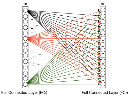
Figure 1 is a network with two fully connected layers with and neurons in each layer respectively. The two layers are denoted as and . Let be one output vector of the layer , where . Let represent the weight matrix of the , where and is the column vector of . Each column is the weight vector of the corresponding neuron in layer . Thus, the output of is given by .
3 Common explanation of convolutional (CONV) layer
There are many tutorials on the convolutional operation in deep learning but most of them are unintelligible for the beginners of deep learning. In this section, we illustrate how to understand and compute the convolutional operation in a matrix multiplication manner. Section 3.1 states the common explanations about the convolutional operation. In convolutional operation, point-wise multiplication is often used for simplicity instead of the convolutional operations shown in Eq (3). The point-wise matrix multiplication for two variables and is shown in the following equation
| (4) |
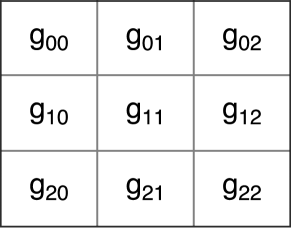
where and are the index, is the filter and is the input patch (i.e. a patch from the whole input with same shape of the filter). For example, to compute the convolution of and in Figure 2 denoted as and respectively, according to Eq (3), . However, in practice, we compute by point-wise multiplication. The difference between convolution and point-wise multiplication is that convolutional operation needs reverse the filter along every dimension.
3.1 Convolutional operation
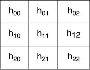
In Figure 3, and are two input and output tensors of CONV layer, where , and , and are height, width and the number of channels respectively. Here we take filters as an example that is shown in Figure 3. Every kernel is of size , where , and are the height, width and number of channels respectively. We use three different colors (i.e. yellow, blue and red in Figure 3) to differentiate these three filters respectively. The dashed lines in Figure 3 depict the convolution operation between the yellow filter and the green patch in and its result is put into the corresponding position (green circle) in . Every filter moves across from left to right and up to down at a step size (also called as stride number). The different color positions in are the output of the kernel with same color. The process is defined as the convolutional operation in CNN denoted as . Let represent the set of the kernels, i.e, where is the number of the kernels (in our example is 3). We can denote .
3.2 Relationship between input shape and output shape
There exists a relationship between the input shape and output shape in the convolutional operation. Stride can be denoted as in the width direction and denoted as in the height direction respectively. Usually, and are set to be the same value so that we can use to represent and . In practice, to get the desired output shape, we often need to pad zeros around the borders of the input. Let denote the number of rows or columns that we want to pad for each side (top and bottom, left and right) . There are three main padding ways, non-zeo padding, half-padding and full-padding (Dumoulin & Visin, 2016). Eq (5), (6) and (7) show the relationships between the input shape and output shape of a convolutional operation:
| (5) |
| (6) |
| (7) |
where /, /, and are the output/input height, output/input width, number of output/input channels and the number of filters respectively.
4 Converting convolutional operation to matrix multiplication
We here extend the analysis of Li et al. (2015) and Gal (2016) (Section 3.4) and give more details about how to convert a CONV layer into a FC layer.
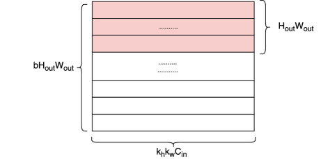
We adopt the convolutional view point as shown in Figure 3. We further assume that and have contained the padding part and the batch size is set to be (or simply think of to be the number of samples). The kernel moves across the spatial space by the stride step . It is equal to extracting patches of size according to the movement of the kernel in the input and then the kernel is convolved or point-wise multiplied with the patches. Each patch can be flattened to a row vector with dimension . These patches constitute a matrix whose dimension is that is shown at the red part in Figure 4a, where and can be got from Eq (5) and (6). This means that each input from the CONV layer can be seen as inputs in a FC layer. The whole matrix in the Figure 4a is denoted as with dimension .
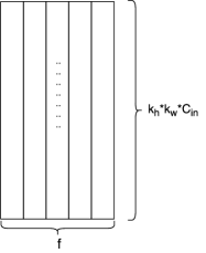
Accordingly, each filter also can be flattened (stretched) to a column vector of shape . Then all the flattened filters make up a filter matrix (i.e. weight matrix in a FC layer) as shown in Figure 4b, denoted as whose dimension is and is the number of the filters. The output is given by whose shape is . In the end, if we want to convert the output of the matrix multiplication back to the output of a CONV layer, we can reshape the result to be of shape .
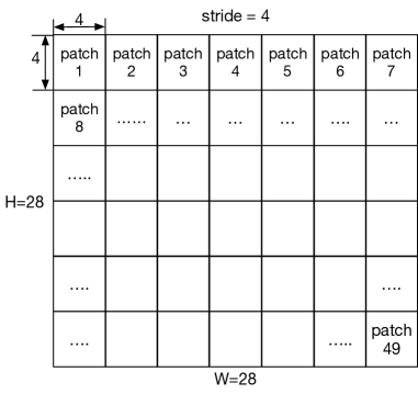
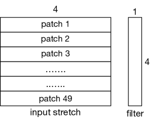
For example, we can get an image of shape from MNIST. We use one filter with shape and set the stride to be to ease the explanation. Figure 6 demonstrates the stretching process and the result. The patches have no overlap because the width and height of the filter are equal to the stride. We can extract patches and each patch is of shape . Then we flatten each patch to a row vector in Figure 6a and stack them vertically together as shown in Figure 6b. The filter is also flattened to a column vector. If there are more than one filter, the flat filters are stacked horizontally.
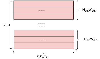
In our experiment, we use as shown in Figure 5 instead of due to the limitation of APIs of Keras. is separated to sub matrices. Each sub matrix is a matrix with shape like the red part in Figure 4a with shape . Then the operation of is divided to the multiplications of sub matrices and .
The process about how to convert convolutional operation to matrix multiplication is described in Algorithm 1, where we assume has already been padded. We also should notice that the index starts from .
In the deep learning framework, the implementation of converting convolutional operation to matrix multiplication is more efficient by a mapping function of index (Vedaldi & Lenc, 2015). The method saves memory. The mapping function describes the relationship of the elements in the matrix of stretching patches and in the input matrix. We here don’t give a detailed example about this which is out of the scope of the article. To simplify the statement, we assume batch size is equal to , i.e., . We know that , where and are the indexes of and , and are the indexes of . is the mapping function of these indexes defined by Eq (8), where , , , , , and and .
| (8) |
5 Experiments
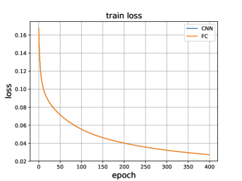
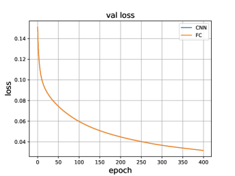
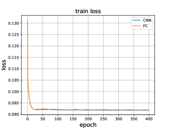
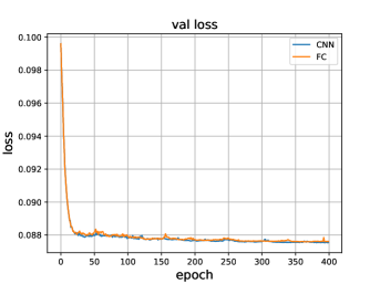
In the experiment, we use Keras to construct one CNN and its equivalent formulation via FC layer (termed as FC network) with the same number of the parameters as shown in Figure 8. We can ignore flatten, activation layers in Figure 8. Both of the networks are going to learn an identity function (i.e. we set the output of the networks to be the original images). For the CONV layer in CNN, the kernel size is set to be and the stride is set to be . The difference between the two networks is that the first layer of CNN is a CONV layer whose filter shape is , but the first layer of FC network is a dense layer of whose weight shape is . We set and use mean square error (MSE) as the loss function. The optimization method is SGD with learning rate. training images and validation images are randomly sampled from MNIST (LeCun et al., 2010) as the training data and validation data. The weight initialization method is set acording to He et al. (2015). To train the FC network, the original input data of shape is converted to the data of shape based on Algorithm 1. We use the same random seed for the two networks so that they have the similar initialization. To simplify the training process, we do not use bias. Both of the two networks are trained for epochs. The training loss curve and validation loss curve are showed in Figure 7. We can see that the training and validation loss curves of CNN and FC network are almost the same via SGD optimization. We also train the two networks via Adam optimization (Kingma & Ba, 2014). We compare the results of two optimization. The code 111Our implementation is available at: https://github.com/statsml/Equiv-FCL-CONVL is available on Github.
One thing we should note as mentioned in Section 4, the input data of images for FC network is actually reshaped to not . It makes no difference and doesn’t affect the weights of the first dense layer in FC network. It just separates matrix to sub matrices and each sub matrix multiplies the weights of shape which is the same if we reshape the data to .


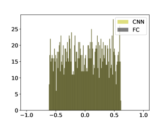
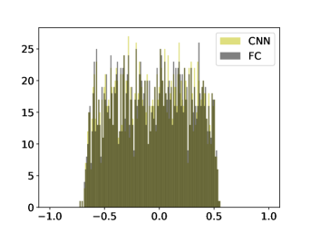
We also extract the outputs of the first layer in CNN and FC network (i.e. the output of conv layer in Figure 8) denoted by and for the CNN and FC network respectively. new images are used to compute and . Then we compute and the result is . Finally, we plot the histograms of the weights of the two conv layers (denoted as and for CNN and FC network respectively) as shown in Figure 9. The histograms from SGD are almost the same for CNN and FC network. And the histograms from Adam almost overlap. We flatten and and their Frobenius norm (F-norm) is . We also tried Adam method to optimize the two networks but the training and validation loss curves of the two networks are not overlapped perfectly like Figure 7 as shown in Figure 10. Adam gets for and F-norm of its flattened and is . It may be caused by the adaptive learning rates for each parameter that is larger update for infrequent and smaller update for frequent parameters.
6 Conclusions
In this note, we illustrate the equivalence of FC layer and CONV layer in the specific condition. Convolutional operation can be safely converted to matrix multiplication, which gives us a novel perspective to understand the convolutional neural network (CNN). And also, in the case where the analysis of CNN is difficult, we can convert the CONV layer in CNN to FC layer and analyze the behavior of CNN in a FC layer manner such as we can analyze the uncertainty in CNN in a FC layer manner.
References
- Blundell et al. (2015) Charles Blundell, Julien Cornebise, Koray Kavukcuoglu, and Daan Wierstra. Weight uncertainty in neural networks. arXiv preprint arXiv:1505.05424, 2015.
- Chen et al. (2015) Tianqi Chen, Ian Goodfellow, and Jonathon Shlens. Net2Net: Accelerating learning via knowledge transfer. arXiv preprint arXiv:1511.05641, 2015.
- Dumoulin & Visin (2016) Vincent Dumoulin and Francesco Visin. A guide to convolution arithmetic for deep learning. arXiv preprint arXiv:1603.07285, 2016.
- Gal (2016) Yarin Gal. Uncertainty in deep learning. PhD thesis, PhD thesis, University of Cambridge, 2016.
- Gal et al. (2017) Yarin Gal, Jiri Hron, and Alex Kendall. Concrete Dropout. arXiv preprint arXiv:1705.07832, 2017.
- He et al. (2015) Kaiming He, Xiangyu Zhang, Shaoqing Ren, and Jian Sun. Delving Deep into Rectifiers: Surpassing Human-Level Performance on ImageNet Classification. CoRR, abs/1502.01852, 2015.
- He et al. (2016) Kaiming He, Xiangyu Zhang, Shaoqing Ren, and Jian Sun. Deep residual learning for image recognition. In Proceedings of the IEEE conference on computer vision and pattern recognition, pp. 770–778, 2016.
- Kingma & Ba (2014) Diederik P. Kingma and Jimmy Ba. Adam: A Method for Stochastic Optimization. CoRR, abs/1412.6980, 2014. URL http://arxiv.org/abs/1412.6980.
- LeCun et al. (2010) Yann LeCun, Corinna Cortes, and Christopher JC Burges. Mnist handwritten digit database. AT&T Labs [Online]. Available: http://yann. lecun. com/exdb/mnist, 2, 2010.
- Li et al. (2015) Fei-Fei Li, Andrej Karpathy, and Justin Johnson. CS231n: Convolutional neural networks for visual recognition. University Lecture, 2015.
- Naghizadeh & Sacchi (2009) Mostafa Naghizadeh and Mauricio D Sacchi. Multidimensional convolution via a 1D convolution algorithm. The Leading Edge, 28(11):1336–1337, 2009.
- Szegedy et al. (2015) Christian Szegedy, Wei Liu, Yangqing Jia, Pierre Sermanet, Scott Reed, Dragomir Anguelov, Dumitru Erhan, Vincent Vanhoucke, and Andrew Rabinovich. Going deeper with convolutions. In Proceedings of the IEEE conference on computer vision and pattern recognition, pp. 1–9, 2015.
- Vedaldi & Lenc (2015) Andrea Vedaldi and Karel Lenc. Matconvnet: Convolutional neural networks for matlab. In Proceedings of the 23rd ACM international conference on Multimedia, pp. 689–692. ACM, 2015.
- Wei et al. (2016) Tao Wei, Changhu Wang, Yong Rui, and Chang Wen Chen. Network morphism. In International Conference on Machine Learning, pp. 564–572, 2016.
- Zhou et al. (2016) Shuchang Zhou, Yuxin Wu, Zekun Ni, Xinyu Zhou, He Wen, and Yuheng Zou. DoReFa-Net: Training low bitwidth convolutional neural networks with low bitwidth gradients. arXiv preprint arXiv:1606.06160, 2016.