DAMPE Electron-Positron Excess in Leptophilic model
Abstract
Recently the DArk Matter Particle Explorer (DAMPE) has reported an excess in the electron-positron flux of the cosmic rays which is interpreted as a dark matter particle with the mass about TeV. We come up with a leptophilic scenario including a Dirac fermion dark matter candidate which beside explaining the observed DAMPE excess, is able to pass various experimental/observational constraints including the relic density value from the WMAP/Planck, the invisible Higgs decay bound at the LHC, the LEP bounds in electron-positron scattering, the muon anomalous magnetic moment constraint, Fermi-LAT data, and finally the direct detection experiment limits from the XENON1t/LUX. By computing the electron-positron flux produced from a dark matter with the mass about TeV we show that the model predicts the peak observed by the DAMPE.
Keywords:
Cosmology of Theories beyond the SM, Dark Matter1 Introduction
One of the signals of a new physics could be the observation of any excess in the energy spectra of the cosmic rays. The search for such an excess in the electron and positron spectra have been already in progress by different particle detectors in the space; the PAMELA satellite experiment observed an abundance of the positron in the cosmic radiation energy range of GeV Adriani et al. (2009), also a positron fraction in primary cosmic rays of GeV Aguilar et al. (2013) and GeV Accardo et al. (2014) and the measurement of electron plus positron flux in the primary cosmic rays from GeV to TeV Aguilar et al. (2014) reported by the Alpha Magnetic Spectrometer (AMS02). The motivation of the current paper is however the recent report of the first results of the DArk Matter Particle Explorer (DAMPE) with unprecedentedly high energy resolution and low background in the measurement of the cosmic ray electrons and positrons (CREs) in GeV to TeV energy range Ambrosi et al. (2017). At energy about TeV a peak associated to a monoenergetic electron source is observed. This excess is interpreted by a dark matter particle with the mass around TeV annihilating into electron and positron in a nearby subhalo in the Milky Galaxy about kpc distant from the solar system. The dark matter annihilation cross section times velocity is estimated to be in the range cm3/ for the aforementioned dark matter mass. For an interpretation of the DAMPE data see Yuan et al. (2017).
There are already several papers that have tried to explain this excess using different models. In Fan et al. (2017) a vector-like fermion DM with a new U(1) gauge boson which only couples to the first two lepton generation is used to explain the DAMPE data. In this direction, model independent analysis performed with fermion DM in Duan et al. (2017a) and with scalar and fermionic DM in Athron et al. (2017). There are also studies within the simplified models with a gauge bosons couples only to the first family of leptons (electrophilic interaction) or to the other families as well Gu and He (2017); Chao and Yuan (2017); Cao et al. (2017); Liu and Liu (2017). There is another study in Chao et al. (2017) where electron flavored fermion DM can interact with the first generation lepton doublet via an inert scalar doublet or with right-handed electron via a charged scalar singlet. In addition, the excess is studied in Hidden Valley model with lepton portal DM Tang et al. (2017), radiative Dirac seesaw model Gu (2017) and gauged model Duan et al. (2017b). It is also studied that the DM particles annihilate to two intermediate scalar particles and then the scalars decay to DM fermions Zu et al. (2017). In Gao and Ma (2017) it is shown that a DM candidate with cascade decay can explain the DAMPE TeV electron-positron spectrum. There are detailed analysis on the morphology of CRE flux considering properties of the primary electron sources Huang et al. (2017a); Jin et al. (2017); Yang and Su (2017).
Meanwhile, it should be noted that there may exist some possible exotic sources for the excess or it may originate from some standard sources like pulsars or supernova remnants. In this work we interpret the excess due to the DM annihilation in a nearby halo.
To explain the DAMPE excess, we come up with a leptophilic dark matter scenario that contains a Dirac fermion which plays the role of the dark matter candidate. Besides, in the dark sector we introduce a gauge symmetry and a complex scalar that together with the Dirac fermion are charged under this gauge symmetry. The dark sector communicates with the standard model sector through two portals. One portal is through the mixing of the complex scalar with the standard model Higgs particle and the other portal comes from the interaction of the gauge boson, , merely with the leptons in the standard model, hence being a leptophilic portal. One of the distinctive characteristics of our two-portal model is that the DM-nucleon elastic scattering begins at one loop level. Therefore there is a large region in the parameter space which evades direct detection. Thus, indirect detection searches become very important tools to probe the viable parameter space of the present model.
In addition to the constraints from the relic density as well as the direct and indirect bounds on the dark matter model, we examine the model if it is consistent also with the new observed DAMPE bump in the electron and positron flux in the cosmic rays.
The paper have the following parts. In the next section we elaborate the setup of our leptophilic dark matter scenario. In section 3 the dark matter relic density and the invisible Higgs decay are computed and compared with bounds from the WMAP/Planck and the LHC. Next we take into account the muon magnetic anomaly and shrink the viable space of parameters. Constraints from the LEP is discussed in section 5. In section 6 we constrain more the model with limits from the direct detection experiments specially the recent XENON1t and LUX experiments. Discussions on the neutrino trident production and decay is given in section 7. We also find a viable space of parameter consistent with the excess observed by the DAMPE in section 8. The Fermi-LAT constraint is discussed in section 9. Finally we conclude in section 10.
2 Model
We explore a leptophilic two-portal dark matter scenario. That is, a fermionic candidate of dark matter connected to the standard model particles through vector and Higgs portals. The vector in the dark sector interacts with all the lepton flavors in the SM but with no interaction with the quarks. The Lagrangian of the model can be written in three parts,
| (1) |
where the dark matter Lagrangian consists of a Dirac fermion playing the role of the dark matter and a complex scalar field both charged under ,
| (2) |
where the field strength is denoted by , the is the Dirac fermion and stands for the complex scalar. The dark sector covariant derivative is defined as,
| (3) |
which acts on the fields in the dark sector as well as the leptons in the SM with being the strength of its coupling and the charge of the field acting on.
Here we study a leptophilic model in which the gauge boson, , interacts only with the leptons in the SM but also with a hypothetical right-handed neutrino for the reason that will be discussed latter on. It is therefore necessary to modify the covariant derivative in the SM to include a term for the new coupling,
| (4) |
where is the coupling in the dark sector and is the dark charge of the leptons that the covariant derivative acts on.
The interaction Lagrangian then reads,
| (5) |
where and are respectively the three families of left-handed lepton doublets and right-handed lepton singlets including the right handed neutrinos. Notice that we have considered universal charges for all families of the leptons, i.e. we have taken the to be the lepton charge for each family of left-handed lepton doublet and to be the charge for and .
Having introduced a new coupled to the dark matter and the chiral fermions in the SM, one must be careful
about the triangle anomalies. In order to remove such anomalies we choose the charges in eq. (5)
to take the following two leptophilic choices,
A)
| (6) |
B)
| (7) |
where is a real number. In the choice A it is assumed that the charge of the lepton and that
of its neutrino are non-zero while in the choice B
we set . We will clarify latter on the reasoning for these choices.
The existence of the right-handed neutrinos are crucial; without them the triangle anomalies can not be fixed. The
charge of the dark matter Dirac fermion, , suffices to have opposite values for its left-handed
and right-handed components, i.e. .
Fixing and substituting the anomaly-free charges in eq. (6) and eq. (7) into eq. (5)
we obtain two interaction Lagrangians,
A)
| (8) |
B)
| (9) |
As seen in eqs. (8) and (9) the vector boson couples to the leptons axially. Note that in eqs. (8) and (9) the fields and are all Dirac fermions. Let us turn back to scalars in the SM and in the dark sector. The Higgs potential as usual is composed of a quadratic and a quartic term which guarantees a non-zero vev for the Higgs field fixed by the experiment to be GeV. After the electroweak symmetry breaking we denote the Higgs doublet as where is the fluctuation around the vev being a singlet real scalar. The complex scalar field, in eq. (2) has two degrees of freedom out of which only one takes non-zero expectation value. The component that takes zero expectation value goes for the longitudinal part of the dark gauge boson. Therefore,
| (10) |
with being a real scalar which mixes with the SM Higgs and the vacuum expectation value of the scalar . The Higgs portal interaction term in eq. (5) together with the scalar potential in eq. (2) and the Higgs potential at the vev of the scalars, leads to a non-diagonal mass matrix for the field space of and . We diagonalize the mass matrix by rotating in the and space by the mixing angle (see Ghorbani and Ghorbani (2015) for more details). After diagonalizing the mass matrix we end up with the physical masses that we denote by , . We are keeping the same notations for the scalar fields and after the mixing. The couplings of the model are in eq. (5), the Higgs quartic coupling in the Higgs potential, and the scalar quartic coupling in eq. (2). These couplings are all expressible in terms of the physical masses, and the mixing angle ,
| (11) |
The vacuum stability conditions on the potential already give rise to the following constraints on the couplings,
| (12) |
The free parameters of the model can then be assigned as , , and .
3 Relic Density and Invisible Higgs Decay
The fermionic DM candidate in the present model is a weakly interacting massive particle (WIMP). The basic vertices to build the diagrams relevant for the annihilation processes are as follows. The DM has a vector-type interaction with , i.e., via the vertex , and the new gauge boson has axial-vector interactions with the SM leptons, i.e., via the vertex . Moreover, there are two types of vertices for the coupled to the SM Higgs and the new scalar, i.e., and . It is therefore possible to have DM annihilation in s-channel via exchange, (for model B, , are absent), as well as in t- and u-channel with a DM exchange, . At temperature higher than the DM mass, the SM particles and the DM candidate are in thermal equilibrium based on the freeze-out paradigm. When the Universe expands the temperature cools down and as a consequence, the DM annihilation rate slows down. There is a temperature we call much below the DM mass where the DM annihilation rate drops right below the Hubble expansion rate of the Universe. At this time, the DM annihilation and production processes are suppressed and the number density of the dark matter remains constant afterwards. The dynamics behind the DM number density evolution is governed by the Boltzmann equation. To obtain the current DM relic density, we make use of the package micrOMEGAs Belanger et al. (2002); Barducci et al. (2018) which solves the equation numerically. The DM annihilation cross sections are computed in CalcHEP Belyaev et al. (2013).
To constrain the model parameters we apply the observed DM relic density Hinshaw et al. (2013); Ade et al. (2014). In addition, to find the viable regions in the parameter space we impose limits on the Higgs invisible decay rate. In the current model, the SM Higgs can decay into and if and respectively. The decay rate for is,
| (13) |
and for the decay it is,
| (14) |
where is a function of the mixing angle and the couplings as,
| (15) |
The Higgs total decay rate will be modified as,
| (16) |
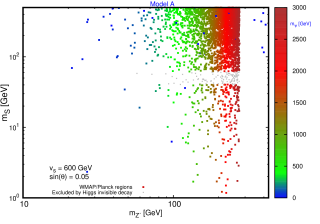
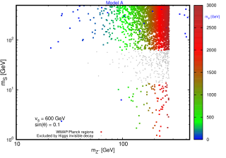
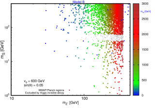
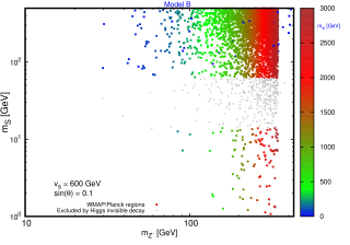
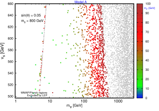
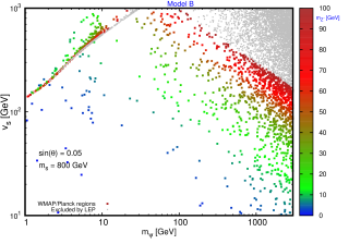
The experimental total decay width of the Higgs obtained in the SM turns out to be MeV. We apply the upper limit on the Higgs invisible branching ratio, Khachatryan et al. (2017). Now for both choices A and B in eqs. (6) and (7) we take GeV and generate random111Throughout the paper scan is carried out using uniformly distributed pseudo-random numbers with linear prior. points in the parameter space with , 1 GeV GeV and 1 GeV GeV. In Figs. 1 and 2 we have illustrated the regions in the parameter space for models A and B respectively, which respect the expected relic density and the regions that are excluded by the experimental limit on the Higgs invisible decay. The results are compared for two different mixing angles and . It is evident from the plots that the excluded regions by the invisible Higgs decay depends strongly on the mixing angle. For the larger mixing angle the scalar masses in the range GeV GeV are excluded, while for the smaller mixing angle scalar masses in the range GeV GeV are excluded. In both cases a wide range of the DM mass are found viable. The mixing angle is fixed at in our analysis hereafter.
4 Muon Anomalous Magnetic Moment
One of the most precisely measured quantity in physics is the muon anomalous magnetic moment. The recent experiment at the Brookhaven National Laboratory (BNL) provides us with its value Bennett et al. (2006),
| (17) |
In the theoretical side, the computation of this quantity is a rather cumbersome task which involves contributions from many processes in QED, QCD and electroweak sectors. Although, the theoretical prediction of this quantity in the SM is affected by some uncertainties in the hadronic low energy cross section and hadronic vacuum polarization, it does not seem possible to explain the observed deviation of around when compared with the recent NBL data: . This deviation may originate from some unknown physics beyond the SM (the new physics) or it could equally arise from some unknown sources in the current physics. When we consider models beyond the SM to explain the shortcomings of the SM, the contribution of the new physics to the muon anomaly should respect the confined bound on . In the present work, only the model A introduces an axial coupling of to the muon and therefore can potentially contribute a sizable amount to as
| (18) |
where Jegerlehner and Nyffeler (2009). In the limit where, , we find
| (19) |
which means that the coupling to the muon makes a negative contribution to the muon anomaly. Given the mass, , will then depends only on the free parameter as
| (20) |
Here we will see that by applying the measured value for , the parameter is constrained strongly such that . Note that there is no bound on the model B from the muon magnetic anomaly.
5 LEP constraint
Leptophilic dark matter models could be restricted by the results of the dismantled Large Electron-Positron Collider (LEP) in the scattering experiment (see e.g. Electroweak (2003); Freitas and Westhoff (2014)). In a model-independent four-fermion effective field theory framework investigation in Freitas and Westhoff (2014) the LEP puts constraint on , the coupling to the electron in eqs. (8) and (9) as,
| (21) |
We note that the mono-photon constraint from LEP is sensitive to light DM mass Fox et al. (2011). The benchmark for our DM mass is TeV. The LEP mono-photon constraint is not relevant since our DM mass is well above the maximum LEP center of mass energy.
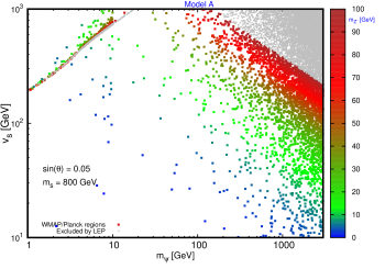
For both models A and B in the current work we have imposed the LEP limits in eq. (21). When considering also the relic density, the invisible Higgs decay and the muon anomaly bounds, the resulting viable space is shown in the Fig. 3. As seen in this figure, for the case A where the muon anomaly selects out the to be only in the range , the DM mass is shrunk into GeV. However for the model B where the muon anomalous magnetic moment is not restrictive the DM mass, , can take values greater than TeV if GeV. For both cases the scalar mass and the mixing angle are fixed at and , respectively. If we relax the constraint on model A, as shown in Fig. 4 the viable parameter space of model A becomes similar to that of model B.
As will be discussed in section 8 it is only the model B that can be tested against the recently observed DAMPE excess. In Fig. 3 the range of the mass has also been shown in color spectrum. It is evident from the figure that the large DM masses can be produced by either very light or heavier ones until GeV.
6 Direct Detection
We consider two types of scattering for the DM in our discussions about direct detection experiments; one is the nucleon-DM scattering and the other one is the DM scattering off the atomic electrons. Let us recall that the DM candidate in our model has a vector interaction with , while has an axial-vector coupling to the SM leptons and no coupling to SM quarks.
Assuming that non-relativistic DM with the mass scatters off the atomic electrons, the electron may be kicked out of the target atom. The elastic scattering cross section at tree-level then reads,
| (22) |
where the suppression factor is the DM velocity in our galactic halo of order . If we plug in the mass the cross section will depend only on as a free parameter, i.e., . The XENON100 experiment results in null result for such a signal, however it puts an upper limit on the elastic cross section as Aprile et al. (2015). This is a rather weak upper limit and as we will see cannot constrain the model parameters.
Now we turn into the nucleon-DM elastic scattering. In the present model this type of scattering can take place via loop induced Feynman diagrams because we deal with a leptophilic DM candidate.
Since the SM Higgs and the scalar both interact with quarks (due to the mixing) and the boson, one type of relevant Feynman diagram for the nucleon-DM elastic scattering is possible as depicted in Fig. 2 in Ghorbani and Ghorbani (2015). In the computation of the scattering amplitude, we use the limit for the momentum transfer. This is reasonable because for a xenon nucleus for instance, we have Ghorbani and Ghorbani (2015). The final result for the spin-independent (SI) elastic scattering in terms of the reduced mass of the nucleon-DM, , reads,
| (23) |
where,
| (24) |
contains the low energy form factors and Belanger et al. (2014), and
| (25) |
with .
Another type of loop induced Feynman diagram which may contribute to the nucleon-DM scattering is the one with charged leptons running in the loop. The lepton loop is connected in one side to the quark current by a photon or a boson exchange and in the other side to the DM current by a exchange. The insertion of the vertex in the lepton loop turns the integral over the lepton momentum into the form,
| (26) |
which is zero due to the odd number of in the trace. Therefore, this process has no effect on the nucleon-DM elastic scattering.
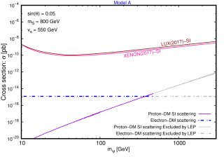
We scan over the parameter space while the mixing angle is fixed at and, to satisfy the constraint from the muon anomalous magnetic moment we choose GeV for the model A. It is chosen GeV for the model B. In both models we choose GeV. It is found out from the results in Fig. 5 that for both models, DM masses up to 3 TeV respect the upper limits on the nucleon-DM cross section imposed by the experiments XENON1t Aprile et al. (2017) and LUX Akerib et al. (2017). However, DM masses larger than GeV are excluded by the LEP in the model A. With the same set of fixed parameters we also compute the electron-DM cross section. Since we have fixed at our analysis and the cross section depends on the this free parameter only, the cross section shows the same behavior in the plots in Fig. 5 and its magnitude in both models is pretty much suppressed and resides well below the upper limit imposed by the XENON100. As seen in Fig. 5, the dark matter mass in model B can take a large range of values from a few GeV to a few TeV after taking into account all the constraints discussed so far.
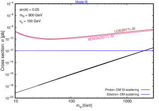
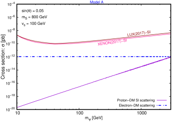
We have also examined the case where the constraint is removed for model A. In Fig. 6 we show our results where the set of parameters in the scan are the same as those for model B. In this case, we find that the viable parameter space respecting the upper limits from direct detections is almost the same as that of model B.
7 Neutrino Trident Production and Decay
Generally, neutrino trident production can constrain models with coupling to both and neutrino Altmannshofer et al. (2014a). It restricts the coupling, , to values given by . For model A, at our benchmark point with TeV, we have GeV while the relevant coupling is . Therefore the neutrino trident production excludes our benchmark point in model A.
Moreover, according to the results in Altmannshofer et al. (2014b) for decay to muons, the region of parameter space at GeV is restricted to couplings in the range . Therefore in model A, our benchmark point with TeV, GeV and is excluded by the decay to muons.
8 DAMPE Excess
The high energy cosmic-ray electrons and positrons (CREs) flux is measured with high resolution and low background by the DAMPE (DArk Matter Particle Explorer) in the range GeV- TeV. The electrons and positrons propagate through the interstellar space and the evolution of their energy distribution, , is governed by the equation
| (27) |
In the above equation the energy loss coefficient is which is parametrized in terms of the energy as with . The diffusion factor, , depends on the energy and the disk thickness, , in the direction of the diffusion zone. It is parametrized as with and . The last ingredient in the diffusion equation is the source function, , for electrons and positrons in the case of DM annihilation. For a Dirac DM candidate the source function is given by
| (28) |
where is the DM mass density, is the velocity-averaged annihilation cross section of the DM and the energy spectrum of per annihilation is denoted by (see Cirelli et al. (2008) for more details).
In case that the energy distribution, , is time independent, the general solution for the energy distribution is given by the integral,
| (29) |
where the space integration is performed over the region of the DM halo and is the energy at the source. The Green function of the diffusion equation is denoted by and understood as the probability to catch an electron or a positron at earth with energy which is produced at point and energy in the DM halo. Finally, the electron and positron flux per unit energy is obtained as , where is the electron or positron velocity.
In this work, to explain the enticing peak in the electron plus positron flux observed by the DAMPE, we assume that there is a DM subhalo nearby with a distance kpc and subhalo radius kpc. For the DM mass density in the subhalo we apply the NFW density profile Navarro et al. (1997)
| (30) |
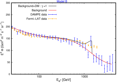
In our numerical computation for the flux the code micrOMEGAs is applied. In order to explain the flux at the peak position of about TeV, we assume the DM annihilation with the mass TeV in the subhalo. We then pick a point in the viable parameter space TeV consistent with the observed relic density and all other constraints. When the scalar mass is fixed at GeV and GeV, the for this benchmark point and GeV.
With the choice of the parameters as and , we are able to explain the observed flux at TeV, as depicted in Fig. 7. The cosmic ray (CR) background is computed in this work by following the formulas in Huang et al. (2017b) for the primary electrons from the CR sources and the secondary electrons and positrons as a result of the primary electrons interaction with the interstellar medium. The relevant parameters in these formulas are obtained by the best fit using the electron plus positron flux measurement by the DAMPE Liu and Liu (2017). We also computed the thermally averaged dark matter annihilation cross section times the velocity at TeV. The result cm3/s is compatible with the dark matter annihilation cross section predicted by the DAMPE. In Fig. 7 we included the Fermi-LAT electron-positron flux Abdollahi et al. (2017) for comparison with the DAMPE data.
In principle the uncertainty on the parameters of the cosmic ray propagation may change our results. For the benchmark point with DM mass TeV we checked this issue and realized that the deviation in our result is negligibly small. This is also in agreement with the conclusions discussed in Belanger et al. (2011).
9 Constraints from Fermi-LAT
The Large Area Telescope (LAT) onboard the Fermi Gamma-ray Space Telescope, was the first to announce an excess in the gamma ray flux at a fairly low energy GeV. The DM annihilation at the Galactic Center was considered as a mechanism to explain the excess. However the latest finding by the Fermi Collaboration, indicates that the excess comes not only from the center of the galaxy but also from regions along the Galactic plane, where a DM signal is not expected Ackermann et al. (2017). Given the assumption that dwarf spheroidal satellite galaxies (dSphs) accommodate a great deal of DM, the Fermi-LAT Collaboration could find the most strong limits on the cross section of DM annihilation into leptons (and quarks) by combined analysis of 15 dSphs in the Milky Way Ackermann et al. (2015).
In the present model, the DM annihilation into is the relevant channel. In this channel, the Fermi-LAT upper bound on the annihilation cross section is most sensitive to DM masses below 100 GeV. Therefore, a DM candidate of mass TeV can evade such upper limits.
One important question is whether the Fermi-LAT have had the possibility to detect a nearby -ray point source mimicking the DM subhalo we considered in the present work to explain the DAMPE excess. In the analysis reported in Yuan et al. (2017) the expected -ray fluxes are calculated for a nearby clump with enhanced DM local density as the ones used to explain the DAMPE excess. In the DM annihilation processes, the -ray may come along with electron-positron ( channel), or from internal bremsstrahlung processes and from decays of final state particles ( channel). In Ref. Yuan et al. (2017) the Fermi-LAT isotropic background data are used to constrain the DM model. It is found that only the -ray emission from the channels exceeds marginally the Fermi-LAT upper limits, and -ray emission from other channels, i.e. channel, respect the Fermi-LAT constraints.
10 Conclusion
The new observed electron-positron excess by the DArk Matter Particle Explorer (DAMPE) may open a window to new physics. The bump reported by the DAMPE in the electron-positron flux is interpreted from a TeV dark matter annihilation to electron-positron from a subhalo in about kpc away from the solar system. The dark matter annihilation cross section times the velocity must be of order cm3/. To explain this excess we introduce a model with a Dirac fermion as the dark matter candidate which has two portals to communicate with the SM, one way is through a complex scalar which mixes with the SM Higgs. And the other portal is through a gauge boson, , interacting with the SM via only the leptons. The charges of the leptons and the dark matter Dirac fermion are chosen in a way to cancel the triangle anomalies. We have investigated two sets of charges once when the muon charge is vanishing and once it is non-zero. We then have computed the relic density and impose its value to be . By the bound from the invisible Higgs decay we restricted more the space of the parameters. The LEP electron-positron collision results, restrict strongly the vacuum expectation value of the scalar and through which the masses of the and the DM. Considering all the bounds above we then have computed the DM-nucleus elastic scattering cross section and constrain the model by the recent direct detection experiments XENON1t/LUX. Constraints from Fermi-LAT observations, neutrino trident production and decay are also discussed. The viable dark matter mass we obtain after imposing all the aforementioned limits contains a TeV dark matter mass which can produce an excess in the electron-positron flux matching the properties of the DAMPE excess.
Appendix A Dark Matter Annihilation Cross Sections
We provide the DM annihilation cross section formulas in this section for four different channels. First, the annihilation cross section for the annihilation process with is obtained as
| (31) |
The other annihilation process is , which is mediated by a gauge boson via s-channel. We find the following result for the annihilation cross section as,
| (32) |
Similarly, we get the DM annihilation cross section for the process ,
| (33) |
Finally, we find the annihilation cross section for the process with a DM particle as the mediator via t- and u-channel,
| (34) |
where in the formulas above, , and are the relevant mandelstam variables.
References
- Adriani et al. (2009) O. Adriani et al. (PAMELA), Nature 458, 607 (2009), arXiv:0810.4995 [astro-ph] .
- Aguilar et al. (2013) M. Aguilar et al. (AMS), Phys. Rev. Lett. 110, 141102 (2013).
- Accardo et al. (2014) L. Accardo et al. (AMS), Phys. Rev. Lett. 113, 121101 (2014).
- Aguilar et al. (2014) M. Aguilar et al. (AMS), Phys. Rev. Lett. 113, 221102 (2014).
- Ambrosi et al. (2017) G. Ambrosi et al. (DAMPE), (2017), 10.1038/nature24475, arXiv:1711.10981 [astro-ph.HE] .
- Yuan et al. (2017) Q. Yuan et al., (2017), arXiv:1711.10989 [astro-ph.HE] .
- Fan et al. (2017) Y.-Z. Fan, W.-C. Huang, M. Spinrath, Y.-L. S. Tsai, and Q. Yuan, (2017), arXiv:1711.10995 [hep-ph] .
- Duan et al. (2017a) G. H. Duan, L. Feng, F. Wang, L. Wu, J. M. Yang, and R. Zheng, (2017a), arXiv:1711.11012 [hep-ph] .
- Athron et al. (2017) P. Athron, C. Balazs, A. Fowlie, and Y. Zhang, (2017), arXiv:1711.11376 [hep-ph] .
- Gu and He (2017) P.-H. Gu and X.-G. He, (2017), arXiv:1711.11000 [hep-ph] .
- Chao and Yuan (2017) W. Chao and Q. Yuan, (2017), arXiv:1711.11182 [hep-ph] .
- Cao et al. (2017) J. Cao, L. Feng, X. Guo, L. Shang, F. Wang, and P. Wu, (2017), arXiv:1711.11452 [hep-ph] .
- Liu and Liu (2017) X. Liu and Z. Liu, (2017), arXiv:1711.11579 [hep-ph] .
- Chao et al. (2017) W. Chao, H.-K. Guo, H.-L. Li, and J. Shu, (2017), arXiv:1712.00037 [hep-ph] .
- Tang et al. (2017) Y.-L. Tang, L. Wu, M. Zhang, and R. Zheng, (2017), arXiv:1711.11058 [hep-ph] .
- Gu (2017) P.-H. Gu, (2017), arXiv:1711.11333 [hep-ph] .
- Duan et al. (2017b) G. H. Duan, X.-G. He, L. Wu, and J. M. Yang, (2017b), arXiv:1711.11563 [hep-ph] .
- Zu et al. (2017) L. Zu, C. Zhang, L. Feng, Q. Yuan, and Y.-Z. Fan, (2017), arXiv:1711.11052 [hep-ph] .
- Gao and Ma (2017) Y. Gao and Y.-Z. Ma, (2017), arXiv:1712.00370 [astro-ph.HE] .
- Huang et al. (2017a) X.-J. Huang, Y.-L. Wu, W.-H. Zhang, and Y.-F. Zhou, (2017a), arXiv:1712.00005 [astro-ph.HE] .
- Jin et al. (2017) H.-B. Jin, B. Yue, X. Zhang, and X. Chen, (2017), arXiv:1712.00362 [astro-ph.HE] .
- Yang and Su (2017) F. Yang and M. Su, (2017), arXiv:1712.01724 [astro-ph.HE] .
- Ghorbani and Ghorbani (2015) K. Ghorbani and H. Ghorbani, Phys. Rev. D91, 123541 (2015), arXiv:1504.03610 [hep-ph] .
- Belanger et al. (2002) G. Belanger, F. Boudjema, A. Pukhov, and A. Semenov, Comput. Phys. Commun. 149, 103 (2002), arXiv:hep-ph/0112278 [hep-ph] .
- Barducci et al. (2018) D. Barducci, G. Belanger, J. Bernon, F. Boudjema, J. Da Silva, S. Kraml, U. Laa, and A. Pukhov, Comput. Phys. Commun. 222, 327 (2018), arXiv:1606.03834 [hep-ph] .
- Belyaev et al. (2013) A. Belyaev, N. D. Christensen, and A. Pukhov, Comput. Phys. Commun. 184, 1729 (2013), arXiv:1207.6082 [hep-ph] .
- Hinshaw et al. (2013) G. Hinshaw et al. (WMAP), Astrophys.J.Suppl. 208, 19 (2013), arXiv:1212.5226 [astro-ph] .
- Ade et al. (2014) P. A. R. Ade et al. (Planck), Astron. Astrophys. 571, A16 (2014), arXiv:1303.5076 [astro-ph.CO] .
- Khachatryan et al. (2017) V. Khachatryan et al. (CMS), JHEP 02, 135 (2017), arXiv:1610.09218 [hep-ex] .
- Bennett et al. (2006) G. W. Bennett et al. (Muon g-2), Phys. Rev. D73, 072003 (2006), arXiv:hep-ex/0602035 [hep-ex] .
- Jegerlehner and Nyffeler (2009) F. Jegerlehner and A. Nyffeler, Phys. Rept. 477, 1 (2009), arXiv:0902.3360 [hep-ph] .
- Electroweak (2003) t. S. Electroweak (SLD Electroweak Group, SLD Heavy Flavor Group, DELPHI, LEP, ALEPH, OPAL, LEP Electroweak Working Group, L3), (2003), arXiv:hep-ex/0312023 [hep-ex] .
- Freitas and Westhoff (2014) A. Freitas and S. Westhoff, JHEP 10, 116 (2014), arXiv:1408.1959 [hep-ph] .
- Fox et al. (2011) P. J. Fox, R. Harnik, J. Kopp, and Y. Tsai, Phys. Rev. D84, 014028 (2011), arXiv:1103.0240 [hep-ph] .
- Aprile et al. (2015) E. Aprile et al. (XENON100), Science 349, 851 (2015), arXiv:1507.07747 [astro-ph.CO] .
- Belanger et al. (2014) G. Belanger, F. Boudjema, A. Pukhov, and A. Semenov, Comput. Phys. Commun. 185, 960 (2014), arXiv:1305.0237 [hep-ph] .
- Aprile et al. (2017) E. Aprile et al. (XENON), Phys. Rev. Lett. 119, 181301 (2017), arXiv:1705.06655 [astro-ph.CO] .
- Akerib et al. (2017) D. S. Akerib et al. (LUX), Phys. Rev. Lett. 118, 021303 (2017), arXiv:1608.07648 [astro-ph.CO] .
- Altmannshofer et al. (2014a) W. Altmannshofer, S. Gori, M. Pospelov, and I. Yavin, Phys. Rev. Lett. 113, 091801 (2014a), arXiv:1406.2332 [hep-ph] .
- Altmannshofer et al. (2014b) W. Altmannshofer, S. Gori, M. Pospelov, and I. Yavin, Phys. Rev. D89, 095033 (2014b), arXiv:1403.1269 [hep-ph] .
- Cirelli et al. (2008) M. Cirelli, R. Franceschini, and A. Strumia, Nucl. Phys. B800, 204 (2008), arXiv:0802.3378 [hep-ph] .
- Navarro et al. (1997) J. F. Navarro, C. S. Frenk, and S. D. M. White, Astrophys. J. 490, 493 (1997), arXiv:astro-ph/9611107 [astro-ph] .
- Huang et al. (2017b) X. Huang, Y.-L. S. Tsai, and Q. Yuan, Comput. Phys. Commun. 213, 252 (2017b), arXiv:1603.07119 [hep-ph] .
- Abdollahi et al. (2017) S. Abdollahi et al. (Fermi-LAT), Phys. Rev. D95, 082007 (2017), arXiv:1704.07195 [astro-ph.HE] .
- Belanger et al. (2011) G. Belanger, F. Boudjema, P. Brun, A. Pukhov, S. Rosier-Lees, P. Salati, and A. Semenov, Comput. Phys. Commun. 182, 842 (2011), arXiv:1004.1092 [hep-ph] .
- Ackermann et al. (2017) M. Ackermann et al. (Fermi-LAT), Astrophys. J. 840, 43 (2017), arXiv:1704.03910 [astro-ph.HE] .
- Ackermann et al. (2015) M. Ackermann et al. (Fermi-LAT), Phys. Rev. Lett. 115, 231301 (2015), arXiv:1503.02641 [astro-ph.HE] .